Detailed Numerical Simulation of Planar Liquid Sheet Atomization: Instability Dynamics, Ligament Formation, and Self-Destabilization Mechanisms

Abstract

The primary atomization of planar liquid sheets near nozzle exits plays a critical role in the study of pressure-swirl atomizers, yet its intrinsic destabilization and breakup mechanisms remain insufficiently characterized due to the multi-scale nature of gas–liquid interactions, significantly limiting the predictive capacity of current widely adopted atomization models. This study utilizes three-dimensional direct numerical simulations (DNSs) with adaptive mesh refinement and the Volume-of-Fluid (VOF) method to examine the instability and disintegration of a spatially developing planar liquid sheet under operating conditions representative of aero-engine combustors (thickness $h=100 \mathsf{\mu }\mathrm{m}$, $We=2544$, $Re=886$). Adaptive grid resolution (minimum cell size $2.5 \mathsf{\mu }\mathrm{m}$) enables precise resolution of multi-scale interface dynamics while maintaining mass conservation errors below 0.1‱. High-fidelity simulations reveal distinct atomization cascades originating from the jet tip, characterized by liquid sheet roll-up, interface expanding, interface tearing, and ligament/droplet formation. Through extraction and surface characterization of representative shed liquid ligaments, we quantify temporal and spatial variations between ligaments propagating toward and away from the jet core region. Key findings demonstrate that ligament impingement on the liquid core serves as the dominant mechanism for surface wave destabilization, surpassing the influence of initial gas–liquid shear at the nozzle exit. Spectral analysis of upstream surface waves reveals a pronounced correlation between high-wavenumber disturbances and the mean diameter of shed ligaments. These results challenge assumptions in classical atomization models (e.g., LISA) by highlighting self-destabilization mechanisms driven by droplet–ligament interactions. This work provides critical insights for refining engineering atomization models through physics-based ligament diameter prediction criteria.

1. Introduction

The liquid atomization process is a complex multi-scale and multi-physics phenomenon that has attracted much attention in the field of computational fluid dynamics. At present, the Eulerian–Lagrangian spray simulation technology [1] is still widely used in engineering applications. As far as the Eulerian–Lagrangian spray modeling method is concerned, the gas is treated as a continuous fluid phase, which can be solved with the Navier–Stokes equation; the atomized droplets are treated as discrete phase, and their trajectories in the gas flow field are tracked by the Lagrangian method. Mass, momentum, and energy source terms need to be considered to fulfill the coupling between discrete and continuous phases.

In this kind of spray modeling method, the real physical and mechanical properties of the dense region near the nozzle exit are ignored completely, and the artificially provided inlet boundary conditions are used instead, where the Lagrangian particles are directly injected at the nozzle exit. The size, spray angle, and injected velocity of these Lagrangian particles are determined from the atomizer model or the primary atomization model [2,3,4,5]. Combined with appropriate secondary droplet breakup models [6,7], droplet evaporation models [8,9], and turbulent combustion models, the complicated spray combustion process can be numerically calculated.

For the commonly used pressure-swirl atomizers, Reitz’s research group proposed the widely used LISA (Linearized Instability Sheet Atomization) primary atomization model by using the linearization theory to mathematically analyze the evolution mechanism of the two-dimensional liquid sheet under the action of infinitesimal disturbances [2,3]. With the proposed LISA model, the wave number and its growth rate of the most unstable disturbance wave can be determined according to the thickness and the injection velocity of the liquid sheet, and the liquid Weber number. Then, the breakup time, the breakup length, and the mean diameter of liquid ligament and droplet (SMD) are computed accordingly. For instance, in the case of short-wave breakup—which specifically refers to instability scenarios where the perturbation wavelength is significantly smaller than the liquid sheet thickness—it is hypothesized that ligament formation occurs through periodic tearing of the liquid sheet at wavelength intervals, representing the predominant destabilization mode observed in swirling liquid sheet breakup mechanisms. Under this assumption, the mean ligament diameter can be expressed as follows:

$$d_{\mathrm{L}}=\sqrt{{\displaystyle \frac{8h}{K_{\mathrm{S}}}}}$$

(1)

where $d_{\mathrm{L}}$ is the mean diameter, $K_{\mathrm{S}}$ is the most unstable wave number, and h is the thickness of liquid sheet.

Since the end of the last century, different atomization models and their variants have been proposed to meet the demands of engineering applications. This kind of Eulerian–Lagrangian spray modeling technology is extensively used in engineering owning to its easy-to-use features. Bhandarkar et al. [10] comprehensively evaluated the predictive ability of different atomization models, especially the secondary droplet breakup model, for the simulation of a high-speed jet in cross flow.

However, to date, no universal primary atomization model has been developed that is applicable to all types of fuel atomizers while maintaining the capability to accurately simulate the primary atomization process in turbulent spray combustion scenarios, thereby providing combustion chambers with sufficiently accurate inlet flow boundary conditions. Even the LISA model, which is specially designed for the atomization description of a hollow-cone liquid sheet, is not capable of truly reflecting the near-field behavior of the atomizers. Before being applied to specific spray combustion problems, the model parameters must be tuned with the help of experimental measurements, which will inevitably limit the use of this model.

To comprehensively understand the intrinsic mechanisms of turbulent spray processes, particularly to elucidate the primary atomization mechanisms near nozzle exits (thereby providing beneficial guidance for establishing engineering atomization models), it is essential that in-depth exploration be conducted into the evolution of gas–liquid interface morphology and the temporal/spatial scales of surface waves during liquid sheet instability and breakup processes. Considering the temporal and spatial scale characteristics inherent to liquid sheet breakup problems, experimental approaches such as high-speed photography currently face significant challenges in investigating the aforementioned atomization mechanisms, whereas numerical simulation emerges as a promising alternative approach. For direct numerical simulation of atomization processes, the following challenges must be addressed:

Firstly, the spatial multi-scale features of the spray field require very high grid resolution and lead to a huge amount of computation costs. Generally, the characteristic length of the combustion chamber is in the order of meters, the size of the nozzle exit is in the order of one tenth of a millimeter, and the liquid ligaments or droplets formed by the jet disintegration are often in the order of tens of microns or even microns. To precisely capture these dynamically changing small-scale liquid structures, it is usually suggested to place 5–10 grid points in the diameter of a liquid ligament or a droplet, which poses a time-consuming challenge for simulating the jet atomization problem.

Secondly, it is hard to calculate the sharp interface between the gas–liquid two phases using many conventional numerical schemes available, which may cause the unwanted interface smoothing phenomenon when used to solve large-density-ratio problems.

With the rapid development of today’s computer resources and parallel solving technology, the first challenge has been gradually solved with the application of local mesh refinements and adaptive solution technology. Hence, lots of researchers have devoted themselves to performing direct numerical simulation of the atomization process by using interface tracking technology. Over recent decades, advances achieved by CFD experts in the domain of interface tracking technologies, including the Volume-of-Fluid method and front-tracking method, have partially addressed the second challenge.

Pan and Suga [11] used the Level-Set method to numerically simulate the circular liquid jet problem, and investigated the jet disintegration in laminar flow state. The simulated jet breakup at a low Weber number is in good agreement with the experimental data, both qualitatively and quantitatively. In Ref. [12], a novel Level-Set/Ghost-Fluid hybrid method with great conservation characteristics was proposed to simulate the incompressible two-phase jet atomization problem, and the computed Reynolds number was 3000.

Shinjo and Umemura conducted a series of studies between 2010 and 2015 utilizing the Level-Set method to investigate circular jet atomization mechanisms. Their work elucidated the following: the formation mechanism of liquid ligaments and droplets [13]; instability characteristics of surface wave-induced atomization [14]; tip-region atomization dynamics [15]; and spectral modulation of droplets/ligaments under turbulent flow effects [16].

Recently, Reddy et al. (2017) [17] conducted a two-dimensional numerical simulation of the atomization process of the thin liquid sheet, and investigated the influence of the jet velocity and the thickness of the thin sheet on the spray angle and droplet distribution. In 2018, Zandian et al. [18,19] used 3D direct numerical simulation to study the instability of a temporally developing planar liquid sheet segment, and achieved the mechanism of liquid breakup and liquid ligament formation/stretching/tearing by analyzing the vorticity dynamics associated with the liquid surface wave dynamics. Three atomization cascades were distinguished during early breakup in their study and a generic diagram was produced that represents all density ratios on a single plot, which identifies the three atomization patterns. The interaction between the liquid film and the incoming air near the pre-filmer and the resulting droplet breakup process were successfully predicted using the Level-Set numerical method in 2018 by Camille Bilger et al. [20], and three remarkable broken modes were identified in their research. Moreover, Schmidt and Oberleithner (2020) [21] investigated the stability of forced planar liquid jets in a quiescent gas environment by utilizing nonlinear simulations and spatial linear stability analysis. By comparing the breakup length, Sauter Mean Diameter (SMD), and spray cone angle, Najafi (2021) [22] examined the impacts of liquid injection pulse frequencies and pressure on the atomization process of a pressure-swirl nozzle. They concluded that an increased pulsation frequency resulted in a reduction in the breakup length and SMD, while spray cone angle remain constant. Pia et al. (2021) [23] examined the frequency response to harmonic disturbances in the transverse velocity imposed on subcritical liquid sheet flows under gravitational influence. Ananth and Trujillo (2023) [24] investigated the instability growth of high-speed liquid sheets injected into a quiescent gaseous environment using the Volume-of-Fluid (VOF) method and spatial linear stability analysis. Their findings demonstrated that the thickness of the gas shear layer is a critical factor influencing instability development, with the dominant sinuous mode being primarily responsible for the fragmentation of the liquid sheet. Furthermore, they highlighted that the growth of the sinuous mode is predominantly governed by the Reynolds shear stress of the gas and the lateral pressure on the gas side.

Regarding pressure-swirl atomizers—widely employed in engineering applications—developing a more sophisticated and generalizable atomization model requires the following: (1) in-depth analysis of liquid sheet destabilization and disintegration mechanisms; (2) quantification of individual contributions from surface wave disturbances to sheet instability; and (3) establishment of quantitative relationships between dominant perturbation waves and resultant ligament diameters. The existing literature reveals that DNSs of spatially developing liquid sheet jets and their disintegration processes remain scarce due to computational constraints and interface-tracking resolution limitations—a knowledge gap that motivates the present investigation. The LISA model implicitly hypothesizes that nozzle-exit-region dominant disturbances govern breakup phenomena. While this assumption requires further validation, the current findings may contribute to refining atomization modeling frameworks.

The structure of this paper is organized as follows. In Section 2, the problem setup and the most important flow parameters are described, followed by the numerical methodology. Grid independence tests are made in Section 3. In Section 4, the results are presented and discussed. The surface instability and the main atomization cascades are investigated firstly. The formation mechanism of liquid ligaments from the liquid sheet tip is discussed in Section 4.2. In Section 4.3, the significance of the impact of ligaments and droplets in the liquid destabilization is explained and determined. Finally, Section 4.4 is given to evaluate the relationship between the dominant wavelength and the mean diameter of the formatted liquid ligaments. The most important findings of this study and future directions are summarized in Section 5.

2. Mathematical Description

2.1. Problem Configuration

The computational domain consists of a cube, as shown in Figure 1. The liquid sheet jet of thickness h ($h=100 \mathsf{\mu }\mathrm{m}$ in the current study, which represents the typical thickness of the liquid sheet at the nozzle exit in aero-engine combustors), which is injected into the computational domain through the nozzle exit, is centered at the middle of the left boundary ($x=0$ plane) of the cubic box. The dimension of the domain in terms of the initial sheet thickness h is $L\times W\times H$ of $50h\times 10h\times 20h$, in the x, y, and z directions, respectively. Given that our focus is placed on liquid injection mechanisms within the immediate vicinity of the nozzle exit region, the influence of gas flow fields in the combustor is assumed to be negligible. Consequently, the liquid jet is surrounded by quiescent air in the computational configuration. Additionally, to achieve compatibility between practical combustor nozzle injection velocities and DNS grid resolution requirements, the liquid sheet is prescribed to propagate at $U=30 \mathrm{m}/\mathrm{s}$ along the positive x-direction (streamwise). Elevated sheet velocities induce reductions in surface wave amplitudes and resultant ligament/droplet length scales, which impose more stringent demands on minimum grid dimensions—collectively increasing computational resource consumption. Fluid properties and flow parameters are given in

Table 1. Fluid properties and flow parameters.

	U	$\rho$	$\mu$	$\sigma$	h
	(m·s−1)	(kg·m−3)	(Pa·s)	(N·m−1)	(μm)
Liquid	30	848	2.87 $\times {10}^{-3}$	$3.0\times {10}^{-2}$	100
Gas	0	34.5	$1.97\times {10}^{-5}$	/	/

in detail. The Weber number and Reynolds number based on liquid properties are 2544 and 886, respectively, which are defined as follows:

$$We={\displaystyle \frac{{\rho }_L{U}^{2}h}{\sigma }},Re={\displaystyle \frac{{\rho }_{L}Uh}{{\mu }_L}}$$

(2)

The flow field is considered to be infinite in the y direction (spanwise). Slip boundary conditions for all components are imposed on the upper and lower sides (in the z-direction) of the computation domain. To mimic the infinite effect in the spanwise direction, periodic boundary conditions are set in the y planes.

2.2. Numerical Methods

In a previous study [25], the authors proposed that the mesh adaptive solution for spatio-temporal multi-scale flows can simultaneously reduce the computational costs and improve the accuracy and resolution of the structures of the transient flow problem. The atomization of a planar liquid jet is a typical multi-scale problem. In the present study, the open-source solver Gerris [26,27] is used to simulate the problem we are interested in. The adaptive solution technology based on the octree grid and the multi-medium interface capture method of VOF are developed in Gerris solver, which is very suitable for the direct numerical simulation of liquid sheet jet atomization. Gerris has been successfully used by the authors to study the mechanism of liquid ligaments and droplets formation in round liquid jets, and satisfactory quantitative and qualitative results have been achieved [28]. In the present study, the visualization analysis of numerical simulation results was performed utilizing ParaView [29].

3. Grid Independence Test

Mesh resolution has a great influence on the accuracy and reliability of numerical simulations. This is especially true for the problems of liquid jet instability and disintegration investigated in this paper. Sufficient grid points have to be placed near the shear layer between the liquid and gas to accurately resolve the growth, destabilization, and breakup behavior of the surface waves. There are a large number of small-scale liquid ligaments, droplets, and holes in the liquid spray structures, which also require sufficiently small-scale grid cells. In addition, the destabilization and disintegration processes of the liquid jet have strong transient characteristics, which will inevitably lead to significant differences in the surface topology at different times.

Considering the temporal and spatial multi-scale features of the liquid sheet jet atomization studied, the mesh adaptive solution approach was utilized, and three grids (M1, M2, and M3) with different refinements were generated in this paper. M1 is a grid with a uniform cell size of 10 μm. In the M1 grid, there are a total of 10 million grid elements, of which 10 grid elements are arranged within the range of the liquid sheet ($h=100 \mathsf{\mu }\mathrm{m}$). M2 and M3 are two sets of adaptive grids, in which the position of grid cells and their element sizes are able to change with the topological geometry of the liquid–gas interface temporally. M2 applied one layer of adaptive refinement, two layers for the M3 grid, and the minimum grid cell sizes corresponding to the two grids are 5 μm and 2.5 μm, respectively. The minimum grid resolution corresponding to M3 is close to the related literature [18,19]. In the study by Zandian et al. [18,19], direct numerical simulations were conducted to investigate the temporal evolution mechanism of three-dimensional instability in planar liquid sheet segments. The thicknesses of the liquid sheet segments were considered as two cases: 50 μm and 200 μm, with the liquid sheet velocity maintained at $U=100 \mathrm{m}/\mathrm{s}$—parameters closely resembling those in the present study. Due to the application of a temporal developing instead of spatial developing approach, their computational costs were relatively lower compared to the simulations performed in this research.

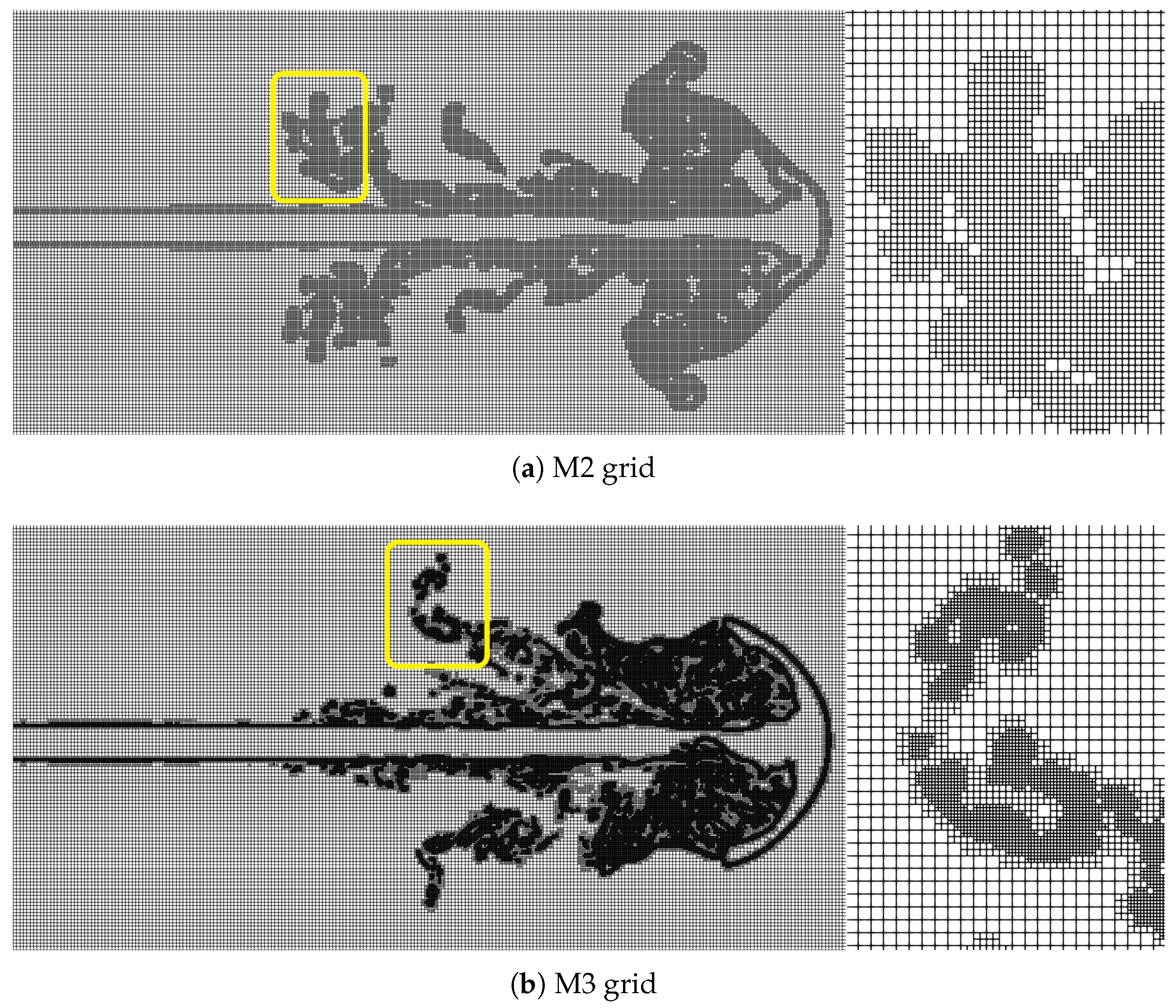
The instantaneous adaptive grids ($t=100 \mathsf{\mu }\mathrm{s}$) along the streamwise section for adaptive solutions based on M2 and M3 are shown in Figure 2, respectively. As can be seen from Figure 2, due to the utilization of the adaptive solution technology, a large number of grid cells are precisely arranged inside the regions where the liquid surface and the broken liquid ligaments/droplets are located. Due to the increase in the number of refinement layers, the jet broken structures resolved by the M3 grid are richer and closer to the actual situation.

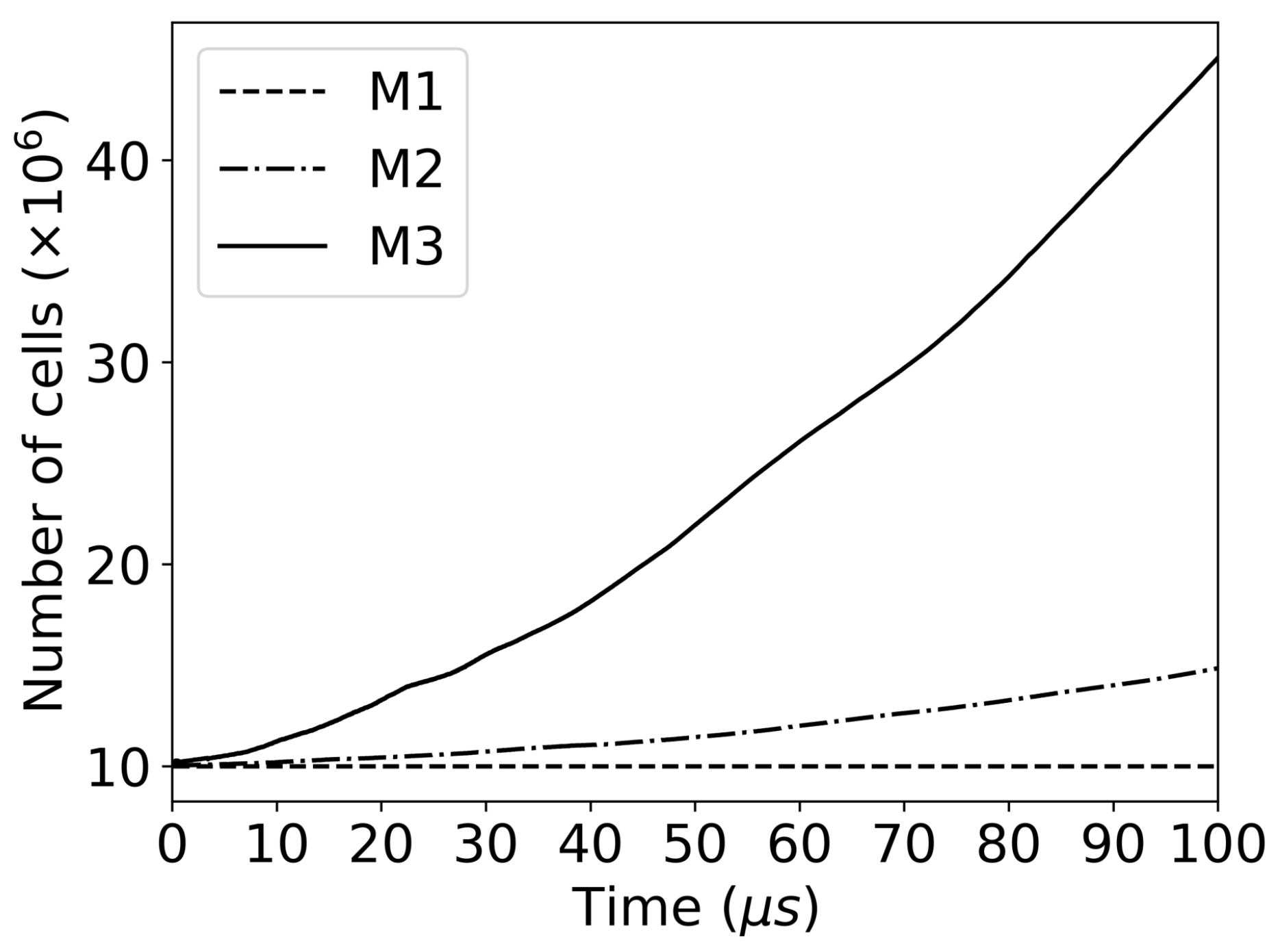
Figure 3 presents the growth of the total number of grid elements over time during the adaptive simulation. The total number of grid elements of the uniform grid M1 is 10 million, while the total number of grid elements of the adaptive grids M2 and M3 increases rapidly with the advancing of time. At $t=100 \mathsf{\mu }\mathrm{s}$, the total number of grid cells for M2 is about 15 million, while the number of grid cells for M3 approaches 45 million. It should be noted that the minimum grid cell size of M3 is approximately $2.5 \mathsf{\mu }\mathrm{m}$. Suppose the present computational domain is subdivided with a uniform grid (minimum grid element size is $2.5 \mathsf{\mu }\mathrm{m}$) instead of an adaptive grid. In that case, we will obtain a grid of up to 640 million elements. Such a large-scale grid system will not only require enormous computing resources and time costs, but also face great difficulties in data analysis and visualization.

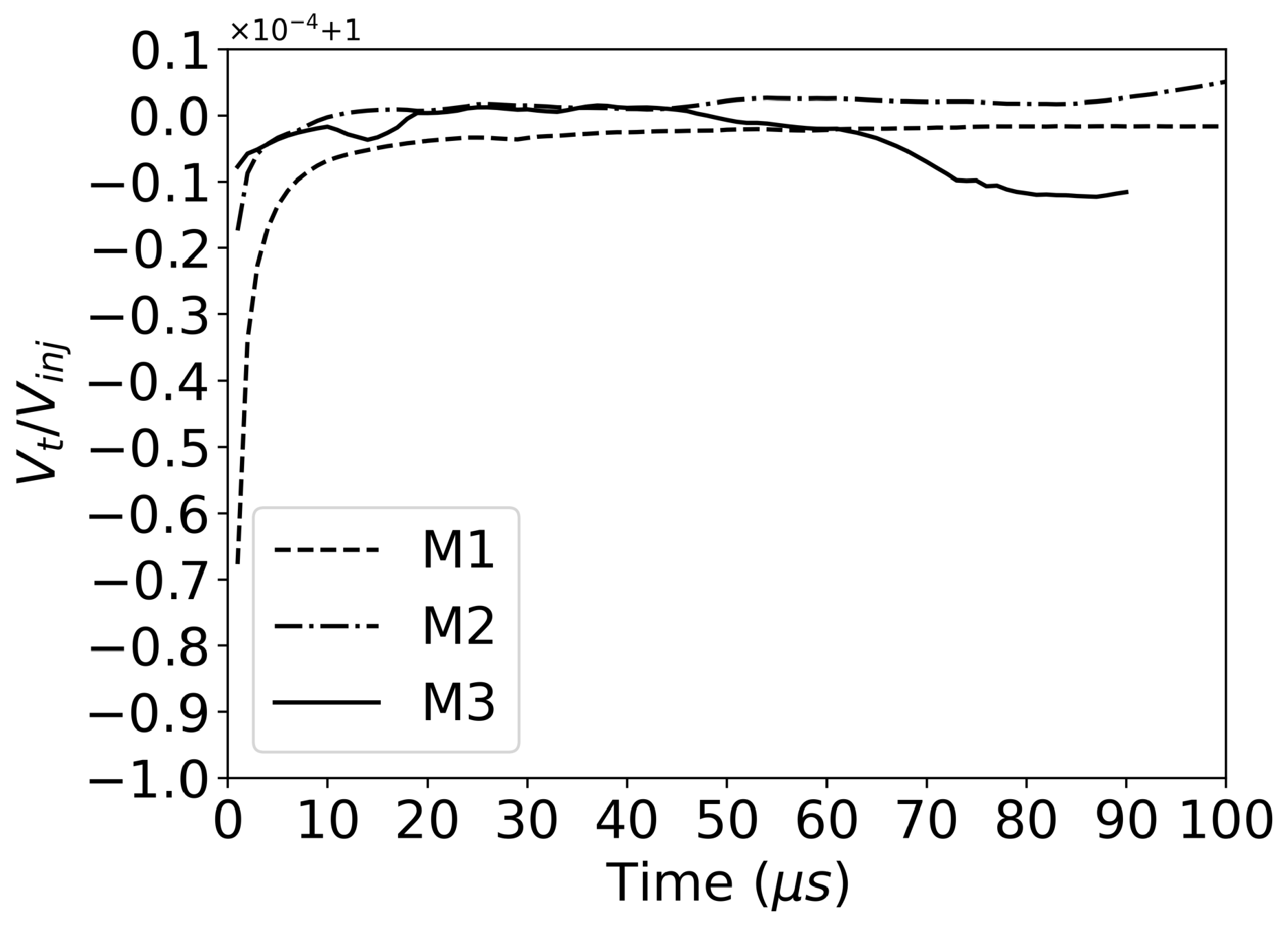
Dissipation and error caused by numerical discretization and interpolation error during the adaptive solution may inevitably lead to the loss of mass within the flow field, and thus affect the capture and identification of a small-scale gas–liquid interface. Hence, more attention must be paid to the issue of mass conservation of flow field in the simulation process. Figure 4 shows the evolution of the ratio of total liquid mass within the computational domain to the total injected mass over time. It can be observed that the mass conservation of flow field at the early stage of calculation is greatly improved due to the application of the adaptive solution technique, and the mass loss is reduced from 0.7‱ to 0.1‱. The mass loss of the whole computational domain is well kept under 0.1‱, even at the late stage when the gas–liquid interface is strongly unstable and broken.

Mesh resolution has a significant effect on the resolved gas–liquid interface structures, as can be seen from Figure 5. Figure 5 shows the gas–liquid interfaces of four typical instants (25 μs, 50 μs, 75 μs, and 100 μs), calculated by the M1, M2, and M3 grids, respectively. The time evolution of the liquid sheet is visualized using ParaView’s volume rendering functionality [30].

It is known that the roll up of the liquid sheet in the streamwise direction and its destabilization in the spanwise direction play a key role in the disintegration and atomization process. From Figure 5, it is observed that all three grids are able to simulate the early roll-up behavior ($t=25 \mathsf{\mu }\mathrm{s}$) very well. Due to the insufficient grid resolution and the resulting numerical dissipation, the shedding of the rolled liquid surface was not clearly captured by the M1 grid, and the spanwise surface instability failed to be induced. Only at the late stage of this simulation ($t=100 \mathsf{\mu }\mathrm{s}$) can weak spanwise surface perturbation be observed in the M1 results. In the simulation results of the M2 grid, the spanwise surface wave is observed earlier, at a time of around $t=50 \mathsf{\mu }\mathrm{s}$. The adaptive solution with the M2 grid successfully captures the three-dimensional destabilization behavior and the formation process of liquid ligaments, but the mesh resolution of M2 is not sufficient to accurately calculate the breakup of liquid ligaments shed from the jet tip.

Thus, in order to meet the demand for mesh resolution, we continue to increase the number of layers of refinements. As can be seen from Figure 5, with M3 grid, the simulation can not only accurately capture the roll up behavior caused by KH instability, but also successfully calculate the generation and growth of spanwise surface waves ($t=25 \mathsf{\mu }\mathrm{s}$). The interaction of the streamwise surface rolls and spanwise surface waves will induce a complex three-dimensional disintegration ($t\ge 50 \mathsf{\mu }\mathrm{s}$), which will finally result in the formation of a large number of liquid ligaments and droplets.

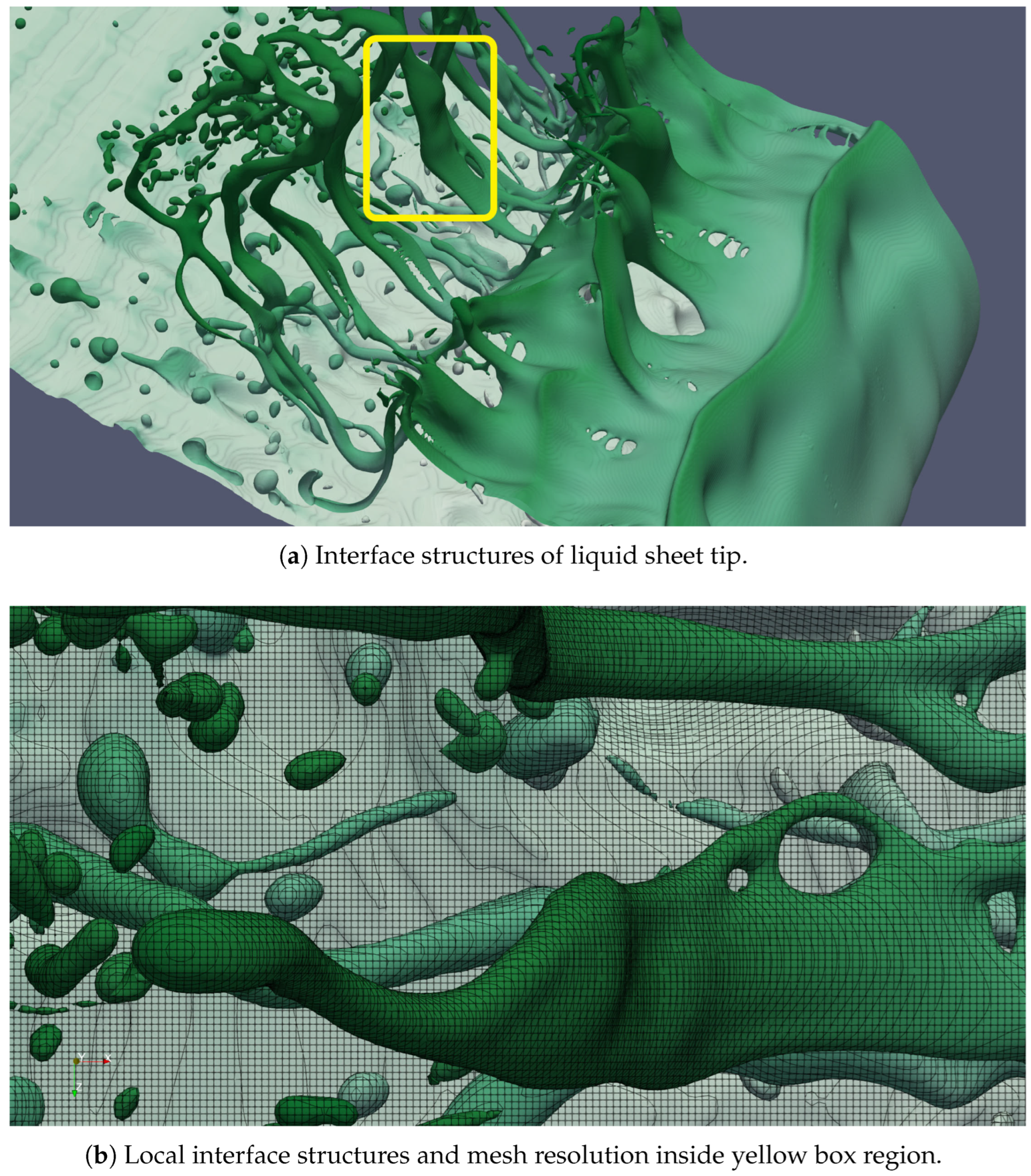
We will further check the grid resolution of the local interface structures. Figure 6a presents the interface structures around the liquid jet tip, which is calculated by the M3 grid. Benefiting from the sufficiently small grid size, the processes of rolling up, stretching, thinning, tearing, and breaking of liquid ligaments, and the droplet formation associated with the liquid sheet tip, can be clearly observed in Figure 6. Moreover, the small-scale structures around the jet tip present smooth shapes, which is consistent with the liquid structure characteristics under the action of surface tension. Figure 6b is a zoomed view of the local small-scale structures, from which typical liquid structures such as ligaments, droplets, and holes can be identified very well. In Figure 6b, most of the ligaments and droplets structures are resolved with more than eight grid cells along the diameter. In their work [13,14,15,31], Shinjo and Umemura et al. proposed that in order to conduct an effective simulation of liquid ligament dynamics, at least eight grid cells have to be arranged along the diameter. From Figure 6b, it is also observed that a few non-physical droplets formed due to insufficient grid resolution. According to the practice of many previous researchers, it is difficult to completely avoid such non-physical droplets, also called digital droplets in numerical simulation, and this remains a common issue. Generally, the number of non-physical droplets can be effectively reduced by using a sufficiently small grid cell size. To fully understand the influence of the presence of non-physical droplets on real fluid dynamics is beyond the scope of the present article.

Figure 7 shows the increase in surface area of the gas–liquid interface, which is calculated by three different grid systems. The following expression is used to describe the liquid surface area increment ratio at time t:

$$(S_t-S_{inj})/S_{inj}$$

(3)

where $S_t$ is the total area of the gas–liquid interface in the calculation domain at time t, and $S_{inj}$ represents the total area of the gas–liquid interface injected into the calculation domain through the nozzle exit within time t without considering the disintegration and atomization of the gas–liquid interface. The value of Expression (3) represents the growth of the total area of the gas–liquid interface in the process of liquid sheet atomization, and a larger value corresponds to a better disintegration effect. It can be seen from Figure 7 that the atomized surface area of the three grid systems presents approximately linear growth at the early stage. The early growing trends of the M2 and M3 adaptive grids are very similar to each other, and approach a local maximum value around $t=10 \mathsf{\mu }\mathrm{s}$. After that, the growth of the surface area shows more nonlinear characteristics due to the intensified three-dimensional instability of the interface. Benefiting from the high grid resolution, finer and richer gas–liquid interface structures (holes, liquid ligaments, droplets, etc.) are resolved in the simulation of the M3 adaptive grid.

Based on the previous discussion, it is concluded that the adaptive solution on the M3 grid is able to precisely calculate the early destabilization and primary atomization process of the liquid sheet jet under current conditions. The results presented in Section 4 are achieved with the M3 grid, if not otherwise stated.

4. Results and Discussion

In Section 4, the authors will focus on the adaptive solution data based on the M3 grid within 0–100 μs to understand the liquid surface dynamic mechanism corresponding to the early instability and primary atomization of the liquid sheet, and try to provide a certain kind of guidance for the establishment of a more accurate correlation model for the prediction of ligament diameter.

4.1. Three-Dimensional Instability and Atomization Cascade

In order to understand the topological deformation of the gas–liquid interface in the process of liquid sheet disintegration, the instantaneous surface of the liquid sheet is visualized every 10 μs with volume rendering technology, as shown in Figure 8.

It can be seen from Figure 8 that in the early stage of the liquid jet ($t<20 \mathsf{\mu }\mathrm{s}$), the K-H instability caused by the gas–liquid shear near the nozzle exit presents an exact symmetry about the center plane. At this time, the spanwise instability is not yet excited, and the fluid structures shed from the rolled-up tip edge of the liquid jet have good two-dimensional features.

When the time approaches $t=30 \mathsf{\mu }\mathrm{s}$, the downstream surface of the liquid sheet jet presents a weak asymmetry about the center plane, and the rolled-up structures shed from both sides of the jet tip begin to show distinct spanwise perturbation. Strip-like liquid ligaments are able to be observed on either side of the rolled-up structures in the spanwise direction. At this point, the liquid sheet jet has completed the initial destabilization process and starts the periodic atomization cascade stage ($t>30 \mathsf{\mu }\mathrm{s}$). It can be seen from Figure 8 that the intensity of the atomization cascade increases with the increase in injecting time.

Figure 9 shows two typical atomization cascades starting at $t=30 \mathsf{\mu }\mathrm{s}$ (left side) and $t=65 \mathsf{\mu }\mathrm{s}$ (right side), respectively (hereafter called cascade A and cascade B, respectively). In order to facilitate the observation of the surface topology of the gas–liquid interface at the jet tip, a top view observation is performed in Figure 9. Through the observation and comparison of these two atomization cascades in Figure 9, we will be able to achieve the main features of the disintegration and spray of the liquid sheet jet.

In the work of Zandian et al. [18,19], the temporal evolution of a planar liquid sheet segment and its breakup mechanism, which is initially superimposed with a certain disturbance, were studied under the action of gas–liquid shear. In their study, liquid deformation and disintegration were only generated from the liquid core region in the flow direction. In the present study, the spatial development process of the liquid sheet jet is calculated, and the simulation results demonstrate clear atomization cascades originating from the tip of the liquid sheet. The so-called atomization cascade mainly includes the following four sub-processes (see Figure 9): (1) rolling up of the large-scale gas–liquid interface structure at the liquid jet tip; (2) expanding and spreading of the rolling-up interface; (3) tearing of the rolling-up interface and formation of liquid ligaments; and (4) stretching, deformation, breakup of liquid ligaments, and droplet formation.

In the atomization cascades, the rolling up, expanding, and spreading of the gas–liquid interface at the liquid jet tip are carried out simultaneously. For cascade A, these processes occur between $t=30 \mathsf{\mu }\mathrm{s}$ and $t=40 \mathsf{\mu }\mathrm{s}$; for cascade B, they occur between $t=65 \mathsf{\mu }\mathrm{s}$ and $t=72 \mathsf{\mu }\mathrm{s}$. The tearing of the rolled-up interface in cascade A starts at the time of $t=40 \mathsf{\mu }\mathrm{s}$, and the distinct liquid ligaments are observed at $t=48 \mathsf{\mu }\mathrm{s}$. However, the tearing of the interface and the formation of liquid ligaments start at $t=72 \mathsf{\mu }\mathrm{s}$ and $t=84 \mathsf{\mu }\mathrm{s}$, respectively, in cascade B.

Comparing cascade A and cascade B, it can be observed that more complicated wrinkling structures with greatly varied amplitudes are involved around the jet tip of cascade B. These wrinkling structures will continue to be stretched and deformed into holes of different scales, and then torn and eventually broken into liquid ligaments. In cascade A, this phenomenon is not clearly captured. Hence, while the primary dynamic behaviors of cascade A and cascade B are similar, they are quite different in terms of the intensity of the disintegration process.

4.2. Formation Mechanism of Liquid Ligaments from Liquid Sheet Tip

After understanding the overall breakup mode of the liquid sheet jet, we will further discuss the instability of the liquid jet tip and the formation mechanism of liquid ligaments. To accomplish this, a detailed description of the surface deformation in a cuboid region with $\Delta L\times \Delta W\times \Delta H$ of $15h\times 5h\times 8h$ is given. Figure 10 presents the interface morphology of the liquid jet tip inside the specified box region at several typical moments to clarify the formation and evolution mechanism of the liquid ligaments. At $t=60 \mathsf{\mu }\mathrm{s}$, the downstream side of the mushroom-shaped tip (pointed at by the red arrow in Figure 10), which impacts the quiescent air in the streamwise direction, appears smooth, and at this moment, it is just in a state of being thrown away from the liquid core region; meanwhile, the upstream interface at the edge of the liquid tip (pointed at by the brown arrow in Figure 10), which is parallel to the direction of the liquid jet and is being thrown towards the liquid core region, is disturbed by the local vortex flow and slight spanwise fluctuations start to appear on it. The liquid ligaments around the jet tip are mainly formed from these two locations, i.e., the downstream and upstream sides of the jet tip, under the action of interfacial instability. Since the temporal and spatial scales of liquid ligaments generated at these two locations are largely different, they are discussed separately below.

The upstream interface at the edge of the mushroom-shaped tip gradually becomes thinner under the stretching of the vortex, and the magnitude of surface fluctuations keeps increasing. The riblet-like and groove-like structures are distinctly identified at $t=66 \mathsf{\mu }\mathrm{s}$. Inside the specified cuboid region, three riblet-like and two groove-like structures can be clearly observed at the tip edges. At $t=72 \mathsf{\mu }\mathrm{s}$, several hole structures are made inside the tip edge due to stretching and tearing, which then evolve into clear liquid ligaments at $t=75 \mathsf{\mu }\mathrm{s}$. The number and the spanwise positions of the riblet/groove structures connecting both ends of the liquid ligaments are not consistent (one end has three riblets and two grooves, and the other end has four riblets and three grooves), which makes the tearing position of the interface at the tip edge not consistent with the position of the riblet/groove structure, though exhibiting a more complex tearing behavior. In the specified region we selected here, a total of about 11 liquid ligaments can be observed at the leading edge of the tip. When the time reaches $t=82 \mathsf{\mu }\mathrm{s}$, it can be observed that the liquid ligaments at the leading edge of the tip start to break up and produce droplets at the broken location. Similar ligament-breaking and the creation of new droplets are also observed at $t=91 \mathsf{\mu }\mathrm{s}$.

Concerning the downstream side of the mushroom-shaped tip, weak surface fluctuations are observed there at $t=70 \mathsf{\mu }\mathrm{s}$, and distinct riblets (4) and grooves (3) start to appear at $t=72 \mathsf{\mu }\mathrm{s}$. At $t=75 \mathsf{\mu }\mathrm{s}$, the holes start to appear at the bottom of the groove structures and gradually evolve into four separated liquid ligaments ($t=84 \mathsf{\mu }\mathrm{s}$). In the time thereafter, these liquid ligaments keep stretching. These liquid ligaments generated at the downstream side of the jet tip are not broken into droplets, until the maximum calculated time ($t=100 \mathsf{\mu }\mathrm{s}$) in this study approaches.

From the above observations, it can be determined that it takes approximately $\Delta t=15 \mathsf{\mu }\mathrm{s}$ for the upstream side of the mushroom-shaped tip to evolve from a weak spanwise fluctuation ($t=60 \mathsf{\mu }\mathrm{s}$) into liquid ligaments ($t$ = 75 μs). This process takes approximately $\Delta t$ = 14 μs ($t=74$∼84 μs) for the downstream side of the mushroom-shaped tip, which is similar to the time for the generation of liquid ligaments at the upstream side of the mushroom-shaped tip. However, it is easy to know from Figure 10 that the diameters of the liquid ligaments produced at these two locations are quite different.

In order to observe the topological evolution of the liquid ligaments generated at the two previously mentioned locations more clearly, two liquid ligaments marked by the green and blue arrows in Figure 10 are extracted and their instantaneous geometries represented with the iso-surface of the volume fraction at several time instants are presented in Figure 11 and Figure 12, respectively.

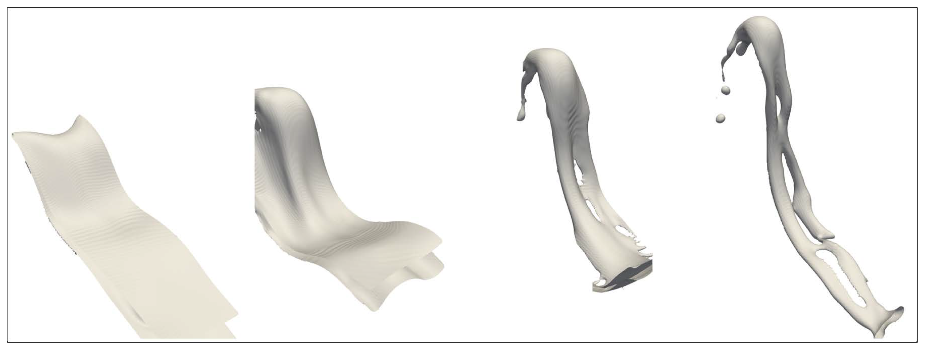
In Figure 11, the diameter of the liquid ligament thrown towards the liquid core region is measured to be about 14.5 μm at $t=77 \mathsf{\mu }\mathrm{s}$; after that, the liquid ligament continues to undergo twisting and stretching, and the surface of the liquid ligament starts to show a distinct periodic wavy structure at $t=87 \mathsf{\mu }\mathrm{s}$. As the time advances, the wave-like bulge becomes more and more apparent, and the neck of the wave-like structures gradually becomes thinner, breaking up at $t=95 \mathsf{\mu }\mathrm{s}$ and $t=99 \mathsf{\mu }\mathrm{s}$, respectively, which leads to the formation of a separated liquid bulb and a droplet with the diameter of about 14 μm.

To further observe the formation process of the liquid ligament thrown away from the liquid core region, see Figure 12. It can be observed that a separate liquid ligament structure is formed at $t=83 \mathsf{\mu }\mathrm{s}$, and the liquid ligament splits and forms two separate child ligaments at $t=91 \mathsf{\mu }\mathrm{s}$. The mean diameter of these two liquid ligaments is about 32 μm.

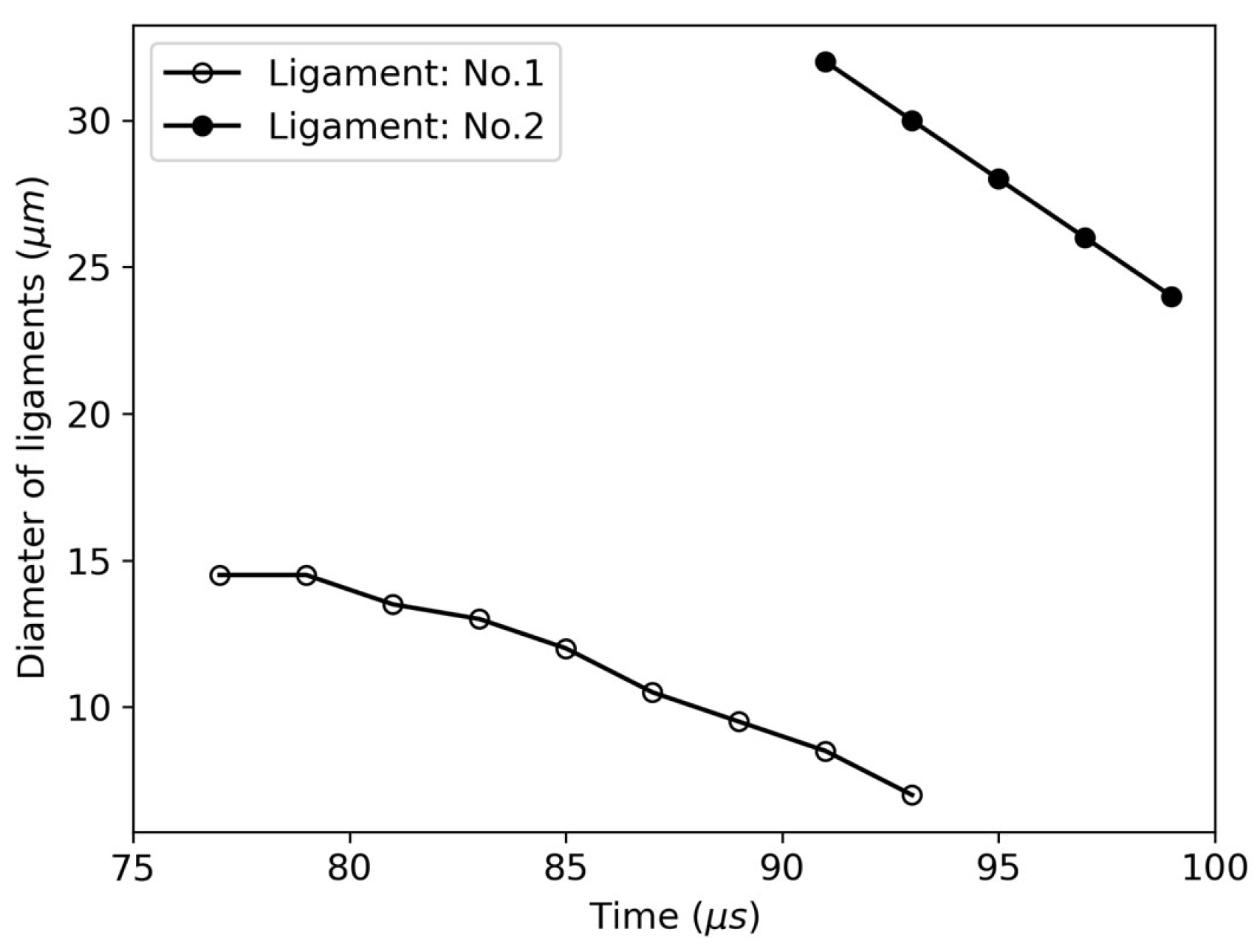
Figure 13 shows the time-dependent curves of the mean diameter of the two liquid ligaments thrown towards and away from the liquid core region. It can be seen from Figure 13 that the rate of change in the diameter of the liquid ligament thrown towards the core region is approximately 0.5 m/s, while the liquid ligament thrown away from the core region has a larger mean diameter, and its rate of change of diameter is also greater, at about 1.0 m/s. The discrepancy in the average diameter change rate of the two liquid ligaments can be attributed to the following mechanisms. For the liquid ligament moving toward the liquid core region, the pressure within the liquid region is relatively high. Consequently, the contraction of the ligament diameter is suppressed by the combined effects of high pressure and liquid sheet flow. In contrast, the liquid ligament ejected outward into the peripheral low-pressure zone experiences amplified surface tension dominance, thereby accelerating radial contraction of the ligament diameter.

Additionally, the evolution process of ligaments formed as a result of the stretching and tearing of the hole structure, as observed in Figure 11 and Figure 12, can be interpreted as the formation of multiple micro-jets. However, unlike a single large-scale jet, the construction of a comprehensive quantitative framework for these multi-scale interactions remains challenging due to the combined effects of liquid sheet flow driving forces and the complex interactions among these micro-jets. Further efforts are required to address this issue.

4.3. Liquid Ligaments/Droplets Impact Behavior and Its Surface Wave Dynamics

In Section 1, it was mentioned that the so-called atomization models are widely used in engineering calculations of two-phase atomization processes. For example, the LISA atomization model [2] is often used to simulate the spray field generated by pressure-swirl atomizers [3]. In developing the LISA model, it is necessary to carry out a linear stability analysis on the deformation process of the two-dimensional liquid sheet under the initial disturbance, and then establish the correlation between the diameter of the liquid ligament and the most unstable disturbance wave. During the linear stability analysis of the LISA model, there is an implicit assumption that the destabilization and disintegration of the liquid sheet are determined by the gas–liquid shear disturbance from the nozzle exit. Through further analysis of the initial destabilization process of the gas–liquid interface, it will be shown that this assumption may not always be reasonable.

In the previous numerical calculations of cylindrical liquid jets [13,14,15,31], researchers observed the impact of droplets shed from the mushroom-shaped tip on the liquid core region, which is important in driving instability and atomization. Accordingly, researchers proposed the so-called self-destabilization mechanism for cylindrical liquid jets [32].

In the present study, the authors will conduct a more detailed analysis of the initial destabilization and breakup process of the liquid sheet jet. Figure 14 shows the surface wave of the liquid sheet jet at different times ($\Delta t=10 \mathsf{\mu }\mathrm{s}$). For the sake of convenience, the outside part of the computational domain beyond 80 μm from the center plane is cut off. Of course, such treatment still cannot completely exclude the isolated liquid ligaments or droplets from the view shown in Figure 14. Thus, special care should be taken to avoid confusion caused by these isolated structures when observing the surface waves in the liquid sheet shown in Figure 14.

It is known from Figure 14 that the surface of the liquid sheet presents a perfect undisturbed shape as $t<20 \mathsf{\mu }\mathrm{s}$. Owing to such a short time, the shear effect between the gas and the liquid has not yet excited the K-H instability. At this moment, the liquid ligaments shed from the jet tip have not yet touched the surface of the liquid core, as shown in Figure 8. It should be noted that the light green colored area in Figure 14 (near the interface roll-up around the jet tip) corresponds to a larger jet speed.

Several remarkable spanwise disturbance structures, which show distinct periodicity along the streamwise direction, are observed in the surface wave structure at $t=30 \mathsf{\mu }\mathrm{s}$ given in Figure 14. These spanwise disturbances are caused by the impact of the periodically shed liquid ligaments from the jet tip on the liquid core at different times. More distinct spanwise disturbances with regular streamwise intervals between them are observed at $t=50 \mathsf{\mu }\mathrm{s}$. The streamwise intervals between these spanwise disturbances are firmly related to the impacting locations of the shed liquid ligaments. These regularly spaced spanwise structures keep propagating downstream, finally leading to the onset of absolute instability of the liquid jet tip. From Figure 8, it is known that at the time of $t=50 \mathsf{\mu }\mathrm{s}$, the liquid ligaments generated from the jet tip are uniformly distributed along the spanwise direction, which is closely related to the spanwise periodicity of the surface disturbances.

At about $t=50 \mathsf{\mu }\mathrm{s}$ (see Figure 9), that is, the ending of cascade A and the onset of cascade B, a large number of liquid ligaments shed from the jet tip start to impact the surface of the liquid core (see Figure 8) and make lots of dents in it. The locations, sizes, and depths may differ considerably between these generated dents. The region inside which the shed liquid ligaments impact the liquid sheet core is identified with a yellow box in Figure 14. These dents are more clearly visible at $t=60 \mathsf{\mu }\mathrm{s}$, and continue to undergo rapid and remarkable deformation during their downstream propagation—see Figure 14. Simultaneously, the rolled-up structures around the liquid jet tip also start to present a more distinct deformation and eventually lead to a more irregular ligament-shedding pattern, such as the shape of the ligaments around the jet tip at the time of $t>70 \mathsf{\mu }\mathrm{s}$, as shown in Figure 8. It is believed that the collision of a large number of shed liquid ligaments with the liquid core was the main reason that caused the destabilization and atomization process, which is similar to the self-destabilization mechanism proposed in Ref. [32].

4.4. Time Evolution and Spectral Characteristics of Liquid Surface Disturbance

In the preceding sections, the topological evolution of the gas–liquid interface in physical space was discussed in detail, and insight into the instability of the surface dynamics and the resulted disintegration behavior was achieved. From the previous analysis, it is known that three kinds of physical effects, namely, (1) the shear at the nozzle exit, (2) the upstream propagation of the impact between the jet tip and still air, and (3) the impact of liquid ligaments/droplets on the liquid core, play roles of varying significance when it comes to the destabilization and self-sustaining atomization of the liquid sheet jet. Which of these three factors is most important in the destabilization of the liquid sheet needs to be further discussed.

In this section, the authors will extract the spatiotemporal and spectral characteristics of the upstream surface wave of the liquid sheet jet and try to evaluate the relationship between the dominant wavelength and the mean diameter of the generated liquid ligaments.

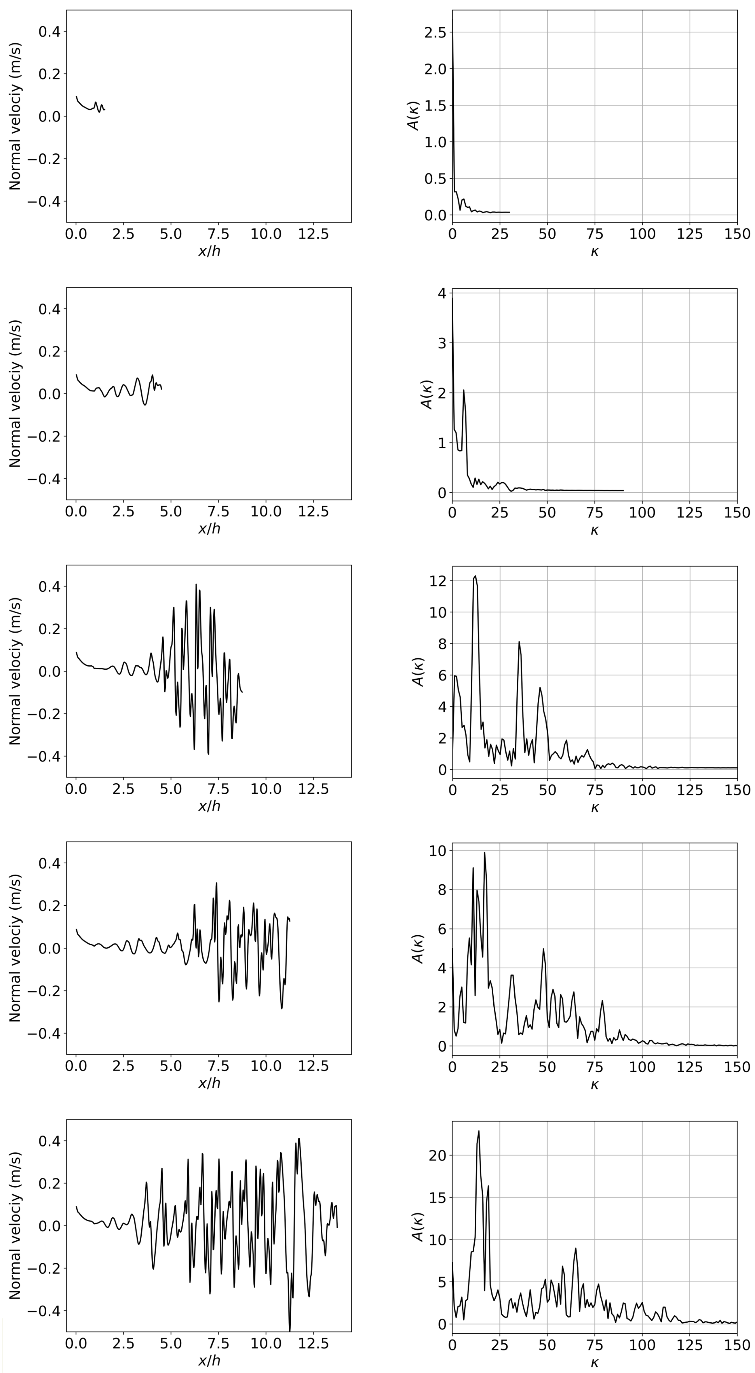
The left column of Figure 15 shows the surface wave disturbance in the core region upstream of the liquid sheet jet at different times, and the amplitude of the disturbance wave is depicted by the normal velocity perpendicular to the center plane. It is observed that before the time of $t=20 \mathsf{\mu }\mathrm{s}$, the disturbance wave on the liquid surface is actually induced by the gas–liquid shear effect starting at the nozzle exit, and the disturbance amplitude is relatively small. According to the analysis in Section 4.3, from the time of $t=30 \mathsf{\mu }\mathrm{s}$, the shed liquid ligaments and droplets start to frequently impact the liquid core region, which is the main contribution to the rapid increase in the disturbance amplitude of the jet surface wave (see Figure 15). As shown in the right column of Figure 15, after $t>40 \mathsf{\mu }\mathrm{s}$, the wave amplitude of the liquid surface disturbances changes more rapidly, and the spectral information tends to be richer. From this time on, those dominated disturbances with high wavenumbers and high amplitudes start to appear successively and compete with each other.

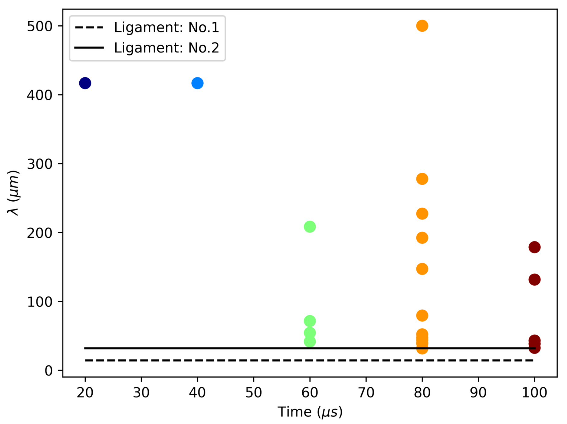
In order to further clarify the correlation between the dominant disturbances and the diameter of the shed liquid ligaments, the wavelengths of the dominant disturbances are plotted as a function of time in Figure 16 ($\lambda =l_{\max }/k$, where $l_{\max }$ is the length of the considered surface wave, and k is the wave number of the dominant disturbance wave). Figure 16 also shows the initial diameters of liquid ligaments thrown away from and toward the liquid core, measuring 32 μm and 14.5 μm, respectively. It can be seen from Figure 16 that these sizes of ligaments are very close to the wavelengths of those high-wavenumber dominant disturbances.

From the analysis of the wavenumber and amplitude of surface waves on the liquid sheet presented above, a significant self-destabilizing mechanism can be observed between the surface wave instability and the impingement of detached ligaments/droplets on the jet core region. The impingement behavior is identified as the predominant factor influencing the destabilization of liquid sheet surface waves. Moreover, a strong correlation is observed between the high-frequency disturbances caused by impingement and the dimensions of detached ligaments, though a definitive mathematical relationship between these parameters has not yet been established and remains an important subject for future investigation.

5. Conclusions

Pressure-swirl atomizers are extensively employed in engineering applications. Liquid sheet jet atomization constitutes a fundamental process in pressure-swirl atomizers. Owing to the intricate physical mechanisms governing the atomization process of liquid sheet jets, establishing a generalized and precise atomization model remains challenging. Current atomization models utilized in engineering computations frequently exhibit limitations in both accuracy and applicability. Consequently, further detailed investigation of liquid sheet jet instability and disintegration mechanisms would significantly contribute to atomization model refinement.

This study elucidates the instability dynamics and primary atomization mechanisms of planar liquid sheets through high-fidelity three-dimensional direct numerical simulations. Key findings are summarized as follows:

(1)

Critical Role of Grid Resolution: Adaptive mesh refinement combined with interface tracking methods was employed to numerically simulate a planar liquid sheet jet under typical operating conditions ($U=30 \mathrm{m}/\mathrm{s}$). Grid independence was rigorously verified. Adaptive mesh refinement with a minimum cell size of 2.5 μm clearly resolved critical features such as ligament thinning and hole formation while capturing intricate interface topologies.

(2)

Multi-Stage Atomization Cascade Dynamics: The liquid sheet exhibited spatiotemporal multi-scale destabilization. Temporal evolution of surface waves revealed periodic atomization cascades originating from the jet tip, comprising four sub-processes: (1) roll-up of large-scale gas–liquid interfaces, (2) expansion and spreading of rolled-up structures, (3) interface tearing and ligament formation, and (4) ligament stretching, deformation, and droplet breakup. Analysis of representative ligaments demonstrated distinct geometric evolution between those propagating toward and away from the jet core, with characteristic scales (14.5 μm vs. 32 μm) and diameter growth rates (0.5 m/s vs. 1.0 m/s).

(3)

Dominance of Self-Destabilization Mechanisms: Contrary to classical atomization models (e.g., LISA), ligament/droplet impingement on the liquid core emerged as the dominant destabilization mechanism. Spectral analysis of upstream surface waves identified high-wavenumber disturbances strongly correlated with shed ligament diameters, suggesting a self-sustaining feedback loop governing instability amplification.

By utilizing adaptive mesh refinement techniques, the high-fidelity simulation results reveal multistage atomization cascades of planar liquid sheets and demonstrate that ligament–core interactions—omitted in classical models—critically modulate instability dynamics through vorticity-driven surface wave amplification and ligament size modulation. Future work will quantify relationships between dominant disturbances and ligament diameters while incorporating nozzle-exit turbulence effects on atomization patterns.