Drivers of Structural and Functional Resilience Following Extreme Fires in Boreal Forests of Northeast China

Abstract

Ongoing climate change has intensified fire disturbances in boreal forests globally, posing significant risks to forest ecosystem structure and function, with the potential to trigger major regime shifts. Understanding how environmental factors regulate the resilience of key structural and functional parameters is critical for sustaining and enhancing ecosystem services under global change. This study analyzed the resilience of forest ecosystems following three representative extreme fires in the Greater Xing’an Mountains (GXM) via the temporal evolution of the leaf area index (LAI), net primary productivity (NPP), and evapotranspiration (ET) as key indicators. A comprehensive wall-to-wall assessment was conducted, integrating gradient boosting machine (GBM) modeling with Shapley Additive Explanation (SHAP) to identify the dominant factors influencing postfire resilience. The results revealed that NPP demonstrated stronger resilience than ET and LAI, suggesting the prioritization of functional restoration over structural recovery in the postfire landscape of the GXM. The GBM-SHAP model explained 45% to 69% of the variance in the resilience patterns of the three parameters. Among the regulatory factors, extreme precipitation and temperature during the growing season were found to exert more significant influences on resilience than landscape-scale factors, such as burn severity, topography, and prefire vegetation composition. The spatial asynchrony in resilience patterns between structural and functional parameters highlighted the complex interplay of climatic drivers and ecological processes during post-disturbance recovery. Our study emphasized the importance of prioritizing functional restoration in the short term to support ecosystem recovery processes and services. Despite the potential limitations imposed by the coarse spatial granularity of the input data, our findings provide valuable insights for postfire management strategies, enabling the effective allocation of resources to increase ecosystem resilience and facilitating long-term adaptation to changing fire regimes.

1. Introduction

The boreal forest in Eurasia is a vital biome for supplying wood products and ecosystem services that benefit human well-being [1]. Ongoing climate warming has profoundly altered natural disturbance regimes in boreal regions, especially because it is anticipated that fire regimes will continue to worsen, which may lead to more severe megafires that pose a major threat to the persistence of boreal forests and ecosystem service supplies [2]. A variety of studies have reported that intensified wildfires have triggered a transition from forests to treeless ecosystems (e.g., tundra, steppe, and shrubland) [3,4], decreased tree coverage and the abundance of needle-leaved trees [5], and changed understory composition [6]. These circumstances reveal a high potential for destabilization in the boreal forest ecosystems in response to severe fire regimes, raising widespread concern. Understanding how boreal forest ecosystems maintain stability after extreme fires is particularly critical for developing mitigation strategies that enhance forest adaptability to warming climates and intensified fire regimes.

Resilience refers to the ability of an ecosystem to maintain its essential processes and functions within the current system domain. It also encompasses the capacity to transition to an alternative ecological equilibrium when necessary [7,8,9]. It has become a crucial and useful concept for expressing the adaptive capacity of an ecosystem in response to changing environments and disturbances [10,11,12,13]. Previous studies have made substantial efforts to quantitatively describe resilience, including identifying characteristics that maintain resilience, proposing surrogate indicators that may indirectly reflect resilience, or developing qualitative and quantitative methods to assess specific aspects of resilience [14,15,16]. Although such efforts have improved our understanding of resilience, several challenges remain in accurately measuring forest resilience to fire disturbances. One significant challenge lies in the inherent variability of fire regimes, which makes the development of universally applicable metrics difficult [17,18]. Additionally, the complexity of ecosystem responses, driven by a multitude of biotic and abiotic factors, further complicates the development of robust and temporally consistent metrics for assessing forest resilience to wildfires [19].

The postfire recovery process can illustrate how forest ecosystems absorb and respond to wildfires, providing a direct and observable framework for assessing forest resilience. Variables that can characterize ecosystem states (e.g., species composition, structural characteristics, and vegetation growth) and ecosystem functions (e.g., nutrient cycling and carbon sequestration) have been adopted to gauge how quickly and effectively a given ecosystem returns to its prefire state or adapts to a new equilibrium [20,21]. Moreover, resilience should be evaluated across appropriate spatial and temporal scales, requiring evaluation metrics with high temporal consistency. However, the unpredictable nature of fire events complicates the collection of consistent, long-term data, which is crucial for measuring resilience [22]. Additionally, forest resilience varies substantially across different locations, highlighting the need to account for spatial heterogeneity when evaluating forest resilience across broader spatial scales [23]. Therefore, remote sensing observations have become central to this effort, given their effectiveness in enabling the continuous monitoring of postfire recovery at the landscape level.

The recovery process in forests is complex and time-dependent; some aspects may be immediate, whereas others may unfold over decades [24,25]. The early period of postfire recovery is critical to drive the direction of succession. The percentages of surviving mother trees (a metric of seed availability), tree seedling attributes (e.g., regeneration success, plant diversity, abundance, postfire vegetation cover and growth conditions) and patterns (e.g., species composition) [26,27] that can be easily observed through field investigations have been widely used to assess forests’ ability to recover. However, field sampling work is labor-intensive and episodic, which may limit data collection and affect the understanding of forest regeneration and ecosystem resilience [28,29]. Remote sensing (RS) enables the observation and retrieval of key parameters related to forest structure and functions, which are widely used to assess ecosystem states. RS-based approaches allow for spatially and temporally continuous tracking of the forest recovery process [30,31], providing a comprehensive evaluation of forest resilience to wildfires, especially to extreme fires. Despite significant efforts to elucidate the patterns and drivers of forest resilience in boreal forests, few studies have focused on monitoring ecosystem structure and function using remote sensing.

The forests in Northeastern China represent the southern margin of the boreal forests on the Eurasian continent and are significantly influenced by global change and wildfires. Research on how forest resilience responds to fires, particularly extreme fires, in this region is crucial for predicting the future dynamics of boreal forest ecosystems and for informing the development of current forest management strategies. Therefore, our objectives are (1) to evaluate forest resilience on the basis of postfire trajectories of ecosystem structure and function via remote sensing, (2) to identify the key drivers that control the spatial heterogeneity of forest resilience, and (3) to demonstrate the relationships between forest resilience and other drivers. To accomplish our objectives, we chose MODIS products to evaluate forest resilience in terms of leaf area index (LAI), net primary productivity (NPP), and evapotranspiration (ET) for the top three largest wildfires in the Great Xing’an Mountains since 2000. Explanatory variables were derived from land cover maps, topography metrics, burn severity estimation, and monthly meteorological observations. We combined the gradient boosting machine (GBM) algorithm and the Shapley Additive Explanation (SHAP) approach to generate a consistent and theoretically sound way to understand variable importance and the impact of individual explanatory variables on forest resilience.

2. Materials and Methods

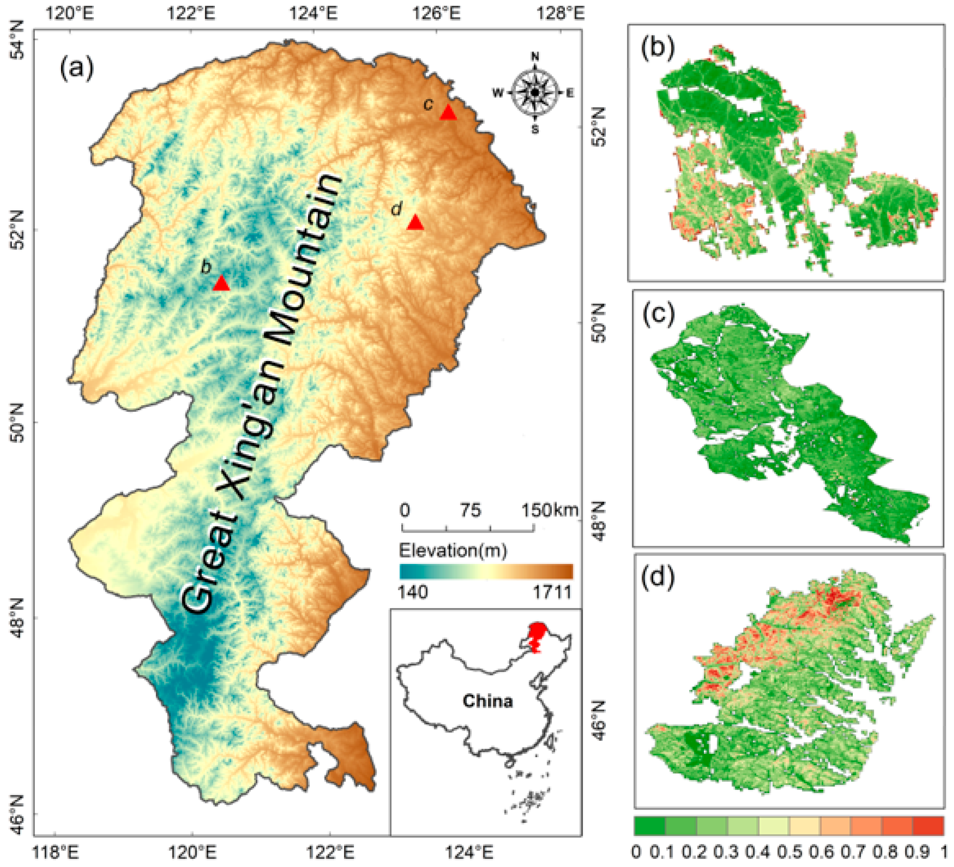
2.1. Study Area

The study was conducted in the Great Xing’an Mountains (GXM) of Northeast China (118.78–127.08° E, 45.69–53.58° N) (see Figure 1), encompassing an area of approximately 25,000 km². This region is characterized by relatively gradual slope, featuring a shallow hilly landscape. The climate is classified as cold temperate continental monsoon, with a mean annual temperature of −1.6 °C, a mean annual precipitation of approximately 472 mm, and a mean annual relative humidity of 70% for the period from 2001 to 2022 [32,33]. The zonal soil of this region is classified as cold temperate brown coniferous forest soil, characterized by a relatively thin soil layer with a high stone content and generally shallow root systems among the tree species [34]. The vegetation of the GXM is characterized primarily by a boreal forest ecosystem dominated by coniferous and mixed forests [35]. In the study area, mature larch forests predominantly thrive in areas with higher moisture levels and cooler climates. In contrast, mixed forests composed of both coniferous and broadleaved species are more commonly found in drier regions with well-drained soils. The prevalent tree species include Dahurian larch (Larix gmelinii (Rupr.) Kuzen), Mongolian pine (Pinus sylvestris var. mongolica Litv.), Siberian fir (Abies nephrolepis), Siberian dwarf pine (Pinus pumila (Pall.) Regel) and Korean spruce (Picea koraiensis Nakai). These conifers are often accompanied by a variety of deciduous species, such as white birch (Betula platyphylla), aspen (Populus davidiana), and Mongolian oak (Quercus mongolica Fisch. ex Ledeb.). In the understory, diverse shrub species contribute to the overall biodiversity of the region, with notable examples including Daurian rhododendron (Rhododendron dauricum), marsh Labrador tea (Rhododendron tomentosum Harmaja), and lingonberry (Vaccinium vitis-idaea L.) [36].

Here, we selected three extreme fires with the largest burned areas since 2000 given their profound consequences for local ecosystems and representativeness as extreme cases for intense fire regimes in the future. Three fires were identified as the Genhe (GH) fire, the Huma fire, and Kanduhe (KDH) fire, respectively (Figure 1a). All three fires occurred during the spring fire season. Due to the extensive scale of these incidents, their origins were subject to official government investigation and public reporting (see

Table 1. Information on the three extreme fire events selected in this study.

Fire Name	Ignition Source	Occurrence Date	End Date	Burned Area (km2)
GH	Human-caused	05/05/2023	11/05/2003	776.55
Huma	Human-caused	22/03/2003	04/04/2003	2729.84
KDH	Lightning-ignited	22/05/2006	03/06/2006	1723.25

). The GH fire was ignited by humans on 5 May 2003 and was suppressed by firefighting teams organized by forestry management on 11 May. Prolonged spring drought coupled with strong winds facilitated the fire spread, causing over 776 km² of forest and meadowlands to experience some form of fire disturbance (Figure 1b). Similar circumstances prevailed during the Huma fire. A four-year consecutive drought and 50-year record low precipitation (~160 mm) dried out the fuels, making them extremely flammable. Crucially, the Huma fire occurred after a period of historical logging, leaving the landscape littered with fine fuels such as non-sprouting dead grass and wood chips, which dramatically increased fire spread, resulting in a fire scar close to 2730 km² (Figure 1c). The KDH fire was ignited by a lightning strike on 22 May 2006, as reported by a government investigation. The prefire landscape in this region is dominated by mixed forests and secondary broadleaved forests resulting from logging activities. Frequent high winds, reduced precipitation (~50–80% below normal as reported), and high temperatures led to rapid fire spread and made suppression by humans more difficult. The fire, though ultimately extinguished by human actions, led to a total burn area surpassing 1723 km² (Figure 1d).

Detailed information related to the ignition sources, occurrence dates, and burned areas can be found in Table 1.

2.2. Ecosystem Resilience Evaluation Using MODIS Products

2.2.1. MODIS Products and Processing

In this study, we evaluated postfire forest resilience from structural and functional properties that can be captured via remote sensing. We adopted the MODIS-derived leaf area index (LAI), net primary productivity (NPP), and evapotranspiration (ET) products as indicators, which can provide insights into canopy structure, physiological activity, and water cycle processes, respectively. The LAI quantifies the leaf area per unit ground area and is essential for evaluating the potential for photosynthesis and water interception [37]. The NPP represents the net rate at which solar energy is converted into biomass, serving as a key metric for ecosystem productivity and carbon sequestration potential [38]. ET includes both plant transpiration and soil evaporation [39] and is a critical determinant of water use efficiency within ecosystems.

Our analysis was conducted at the annual interval and 500 m spatial resolution on the basis of the trade-off between data availability and consistency in spatiotemporal characteristics. We used the latest versions (V6.1) of MOD15A2H (https://lpdaac.usgs.gov/products/mod15a2hv061/) (accessed on 25 December 2024), MOD17A3HGF (https://lpdaac.usgs.gov/products/mod17a3hgfv061/) (accessed on 25 December 2024) and MOD16A2GF (https://lpdaac.usgs.gov/products/mod16a3gfv061/) (accessed on 25 December 2024) to obtain the inter-annual changes in the LAI, NPP, and ET from 2001 to 2022, respectively. Two 8-day products, MOD15A2H and MOD16A2GF, were further processed into annual intervals as the NPP product on the basis of the maximum value compositing method to minimize the impact of null and outlier values. The MVC method was chosen to prioritize the capture of peak vegetation activity during the growing season, which is critical for assessing postfire recovery dynamics. This approach not only reduces the influence of cloud contamination and low-quality observations but also retains the original data values, ensuring that the results reflect actual vegetation conditions without introducing artificial smoothing or distortion. While this method has its limitations and may not be universally applicable, it provides a reasonable and practical solution for capturing vegetation dynamics in postfire resilience studies.

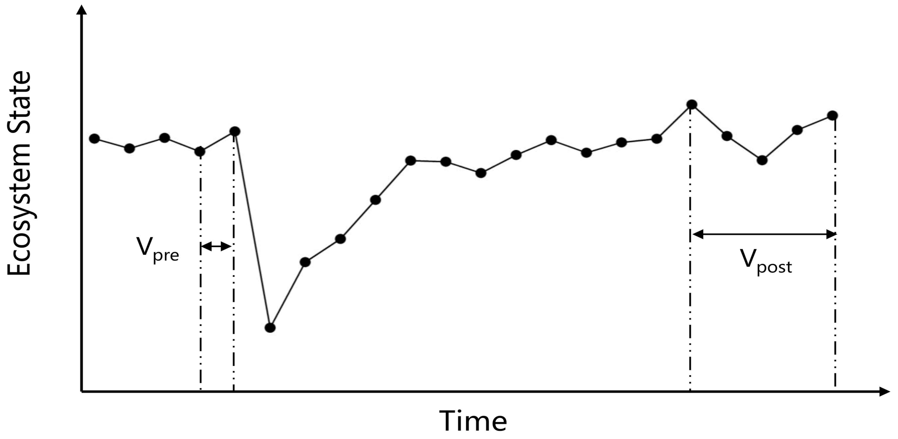
2.2.2. Ecosystem Resilience Evaluation Model

We defined resilience as the capacity of an ecosystem to revert to its prefire state or to realign and stabilize under new conditions following a perturbation. An ecosystem exhibiting high resilience can swiftly regain its key functions and structures postfire or adapt to novel environmental conditions by establishing a new equilibrium. We adopted a resilience quantification approach proposed by Yi and Jackson [18] to analyze how forest ecosystems respond to fire disturbances from a time series analysis of ecosystem state changes (see Figure 2).

To establish a baseline of prefire ecosystem states, for each burned pixel, we used the mean annual values of the surrogate variables (i.e., NPP, LAI or ET) two years before fire occurrence as proxies of the stable prefire ecosystem state (denoted as V_pre). The recovery state was measured as the average value of the postfire years, which ranged from 12 to 16 years depending on the data availability (denoted as V_post). The resilience was calculated using the following model:

$$\mathrm{Resilience}=(\mathrm{V}\mathrm{post}-{\mathrm{V}}_{\mathrm{pre}})/{\mathrm{V}}_{\mathrm{pre}}$$

(1)

where V_pre and V_post are the average values of the state variables prefire and postfire, respectively. A larger resilience value indicates greater resilience, suggesting a better recovery capacity of ecosystem functioning or structure within a given time period.

2.3. Explanatory Variables to Model Forest Resilience

We selected several explanatory variables to represent the influences of prefire vegetation composition, topography, burn severity, and climate on forest resilience. These explanatory variables were primarily derived through a re-analysis of publicly available datasets or open-source Landsat imageries.

2.3.1. Prefire Vegetation Composition

The vegetation composition prior to disturbance is a critical factor determining the resilience of a given ecosystem. We obtained the prefire vegetation composition from a global landcover-dynamics-monitoring product called GLC_FCS30D, which has been validated with an overall accuracy of 73.4% for 17 land cover classification system (LCCS) types [40]. It was developed from a Landsat time series via a revised continuous change-detection (CCD) algorithm. We used the GLC_FCS30D dataset from 2002 and 2005 to determine the coverage of the dominant vegetation types for the Genhe and Huma fires and the KDH fire, respectively, which included deciduous broadleaved forest (DBF), deciduous needle-leaved forest (DNF), evergreen needle-leaved forest (ENF), and grassland shrubs (GRASSs). For each fire year, we used a 16 × 16 moving window analysis to calculate the proportion of all vegetation types and then further resampled them to a resolution of 500 m using the bilinear interpolation algorithm. These classifications are not only indicative of the ecosystem’s initial state but also reflect their varying susceptibilities to fire, which directly influences the subsequent recovery dynamics.

2.3.2. Topography

Topographic features significantly modulate local hydrothermal regimes, soil characteristics, and vegetation distributions and thus control the postfire trajectory of forest recovery [41]. The Shuttle Radar Topography Mission (SRTM) DEM with a 30 m spatial resolution was obtained from the United States Geological Survey (USGS). We first used spatial aggregation with a 16 × 16 focal window size to obtain the maximum elevation at a resolution of 480 m and then applied nearest neighbor resampling to produce a DEM at a resolution of 500 m. On the basis of the aggregated SRTM DEM dataset, we derived several variables, such as elevation, slope, and potential solar radiation (PSR), to evaluate the effects of topography on resilience. The elevation represents the maximum altitude within a 500 × 500 pixel, while the slope is calculated in degrees. The PSR was calculated to indicate the energy input to the ecosystem, reflecting the potential for photosynthesis and biomass accumulation, following the following equation:

$$\mathrm{PSR}=\cos (\mathsf{\theta }-225)\times {\displaystyle \frac{\mathsf{\pi }}{180}}$$

(2)

where θ is the aspect in degrees. Higher PSR values indicate greater potential solar insolation.

2.3.3. Burn Severity

Burn severity is treated as a key metric for determining forest resilience to wildfires through several mechanisms, such as legacy effects and immediate disturbance impacts [42]. To map the spatial extent and burn severity of the three fires, we acquired a series of pre- and postfire Landsat images with the least cloud coverage within the growing season (see

Table 2. Landsat TM image acquisition dates used to map the burned area and burn severity.

Fire Name	Path/Row	Prefire Image Date	Postfire Image Date
GH	122/24	26/07/2002	11/06/2003,
Huma	120/23	26/06/2002	02/08/2004
KDH	120/24	02/06/2005	08/08/2006

). We chose images of the fire occurrence year or the second year postfire on the basis of cloud-free data availability to delineate the burned area via a combination of NBR thresholding and visual interpretation [35]. For burn severity evaluation, we focused on imagery from 1 to 2 years postfire to capture the early stages of ecological recovery. To improve the consistency of burn severity evaluation among fires, we carefully chose cloud-free Landsat images with a particular emphasis on the temporal consistency between pre- and postfire images, as well as the temporal consistency in image selection across different fires. Table 2 presents the pre- and postfire Landsat surface reflectance imagery utilized in this study to delineate the burned area and evaluate the burn severity for three fires.

To generate consistent burn severity evaluations across fires in different locations and times, we used a relative version of the difference normalized burn ratio (RdNBR) index. This index was derived from Landsat images and helps mitigate the incomparability problem caused by heterogeneous prefire landscapes. The RdNBR can calibrate differences in prefire vegetation type and density, providing a standardized assessment across multiple fire events [43,44]. It was calculated via Equations (3) and (4):

$$\mathrm{R}\mathrm{dNBR}=({\mathrm{NBR}}_{\mathrm{pre}}-{\mathrm{NBR}}_{\mathrm{post}})/\sqrt{\left|{\mathrm{NBR}}_{\mathrm{pre}}\right|}$$

(3)

$$\mathrm{NBR}=(\mathrm{NIR}-\mathrm{SWIR})/(\mathrm{NIR}+\mathrm{SWIR})$$

(4)

where NIR and SWIR represent the surface reflectance of the near-infrared and shortwave infrared bands of Landsat, respectively. We first used the median RdNBR value within a 16 × 16 moving window to generate a general burn severity estimation and then resampled it to a resolution of 500 m via the bilinear interpolation algorithm to match the spatial resolution of the other data.

2.3.4. Climatic Factors

Climatic conditions are pivotal drivers or stressors that influence postfire ecosystem restoration in many ways. We acquired monthly air temperature and precipitation datasets and yearly aridity index datasets from the National Tibetan Plateau Data Center of China at a 1 km spatial resolution for the period 2001–2022. The aridity index was calculated as the ratio of annual potential evapotranspiration to annual precipitation, which was used to characterize the hydrothermal conditions. All the climatic datasets were also resampled to 500 m using the bilinear interpolation algorithm to match the abovementioned datasets. We derived climatic variables from several aspects, such as extreme conditions, trends, and average conditions of the growing season for the postfire time periods (i.e., 16 years), to reflect the regulation mechanisms of climatic variation. The maximum or minimum values within the growing season were adopted to reflect potential influences from extreme climatic conditions. We used the Mann–Kendall (MK) test, a nonparametric and rank-based test, to determine and quantify monotonic trends of annual statistics aggregated from monthly time series. For the overall trends of temperature and precipitation, we used the seasonal Mann–Kendall (SMK) test, which is a modification of the MK test that is designed to handle seasonal data, to process the monthly time series. We used Sen’s slope estimate to measure the magnitude of monotonic trends at the pixel level.

2.3.5. Explanatory Variables

Here, we classified the abovementioned explanatory variables into four groups to illustrate the associations of topography, burn severity, prefire vegetation composition, and climatic factors with forest resilience. All variables are shown in

Table 3. Explanatory variables analyzed in resilience models.

Types	Variable Name	Description and Processing
Topography
	Elevation	Altitude of given pixel above sea level derived from SRTM
	Slope	Steepness or incline of the terrain in degrees
	PSR	Amount of solar energy that could be received by a surface; the southwest-facing slopes receive more solar radiation
Burn Severity
	RdNBR	Median value of RdNBR represents fire-caused ecosystem changes
Prefire Vegetation Composition
	DBF	Proportion of deciduous broadleaved forest before fire
	ENF	Proportion of evergreen needle-leaved forest before fire
	DNF	Proportion of deciduous needle-leaved forest before fire
	SBG	Proportion of shrub- and grassland before fire
Climatic Factors
	PRE_SMK_SLOPE 1	Rate of change in monthly precipitation within 16 years postfire
	TMP_SMK_SLOPE 1	Rate of change in monthly mean temperature within 16 years postfire
	Mean_AI	Mean aridity index within 16 years postfire to indicate the average status of dryness
	Max_AI	Maximum aridity index within 16 years postfire to indicate the most extreme dryness condition
	Trend_AI 2	Rate of change in annual aridity index within 16 years postfire
	Mean_maxpre	Mean status of maximum precipitation in growing season derived from the annual maximum precipitation within 16 years postfire to indicate extreme moist condition
	Trend_maxpre 2	Rate of change in annual maximum precipitation during growing season within 16 years postfire
	Mean_minpre	Mean status of minimum precipitation in growing season derived from the annual minimum precipitation within 16 years postfire to indicate extreme dryness condition
	Trend_minpre 2	Rate of change in annual minimum precipitation during growing season within 16 years postfire
	Mean_maxtmp	Mean status of the highest air temperature in growing season derived from the annual maximum temperature within 16 years postfire to indicate extreme heat condition
	Trend_maxtmp 2	Rate of change in annual maximum temperature during growing season within 16 years postfire
	Mean_mintmp	Mean status of minimum temperature in growing season derived from the annual minimum temperature within 16 years postfire to indicate extreme cold wave or frost event
	Trend_mintmp 2	Rate of change in annual minimum temperature during growing season within 16 years postfire

Notes: ¹ Trends of given variables, in terms of Sen’s Slope, were derived from seasonal Mann–Kendall test using monthly inputs variables. ² Trends of given variables, in terms of Sen’s Slope, were derived from Mann–Kendall test using yearly statistics.

.

2.4. Statistical Analysis

2.4.1. Gradient Boosting Machine Modeling

We used a data-driven approach, the gradient boosting machine (GBM) algorithm [45], to find relationships between forest resilience and explanatory variables. The GBM algorithm employs a robust ensemble technique to fit a predictive model by iteratively refining weak learners through gradient descent optimization [46]. It adopts a recursive partitioning mechanism to split training data and construct an ensemble of classification and regression trees (CARTs) sequentially to minimize residual errors of the previous trees. This strength can support the ability of the GBM algorithm to handle nonlinear relationships and complex joint effects among explanatory features. In addition, it can mitigate overfitting problems by adjusting key hyperparameters (i.e., the number of trees, learning rate, tree depth, and subsampling rate) on the basis of a multiple-fold cross-validation procedure. The performance of the fitting power was evaluated via the coefficient of determination (R²) and root-mean-squared error (RMSE) derived from the linear regression using the internal observations against the fitted model.

To ensure generalizability and stable performance on the validation datasets, we randomly selected 10,000 burned pixels to build training data. This dataset contains structural and functional resilience values derived from NPP, ET, and LAI time series and corresponding explanatory variables related to vegetation, topography, burn severity, and climate. The training data were split into two parts, among which 70% were used to train the model and the rest were used for accuracy validation. In this study, we set these parameters at 0.01, 5 and 0.5, respectively, as we previously reported [37]. The number of trees in each GBM trial was automatically selected via a 5-fold cross-validation procedure.

2.4.2. Shapley Additive Explanation

Although the GBM can provide high predictive accuracy, the complexity of these models can often obscure the underlying relationships between features and the target variable. Here, we combined GBM modeling with the Shapley Additive Explanation (SHAP) approach to construct highly accurate and interpretable models. SHAP can enhance our understanding of GBM modeling through improving model accuracy and interpretability on the basis of the SHAP value derived from cooperative game theory. The SHAP values serve as a quantitative measure of each feature’s impact, with the positivity or negativity of these values indicating an enhancing or diminishing prediction, and the magnitude reflects the strength of their influence [47]. The SHAP approach considers all possible coalitions of explanatory variables and computes the average marginal contribution of each variable.

Here, we used the SHAP value to measure the influence of explanatory features on resilience. We noted that when collinearity exists among explanatory variables, the SHAP algorithm tends to assign high SHAP values to variables with greater explanatory power for the GBM model. Meanwhile, it will treat the remaining variables as redundant information and assign them low or even zero SHAP values. Given the ubiquitous presence of collinearity in natural sciences, and to balance model performance with the retention of ecologically significant variables, we employed SHAP value ranking to exclude the six least influential predictors. Furthermore, we focused our discussion on the driving mechanisms of the six highest-ranked explanatory variables, i.e., those with high confidence. In addition, we used a partial dependence plot (PDP) to visually interpret how a specific variable influences the GBM predictions while holding other variables in the model constant. We used the “gbm3” (version 2.2), “shapviz” (version 0.9.3), and “raster” (version 3.6-26) packages in R 4.3.1 (R Development Core Team 2023, Boston, MA, USA) to perform the driver analysis for resilience related to NPP, ET, and LAI, respectively.

3. Results

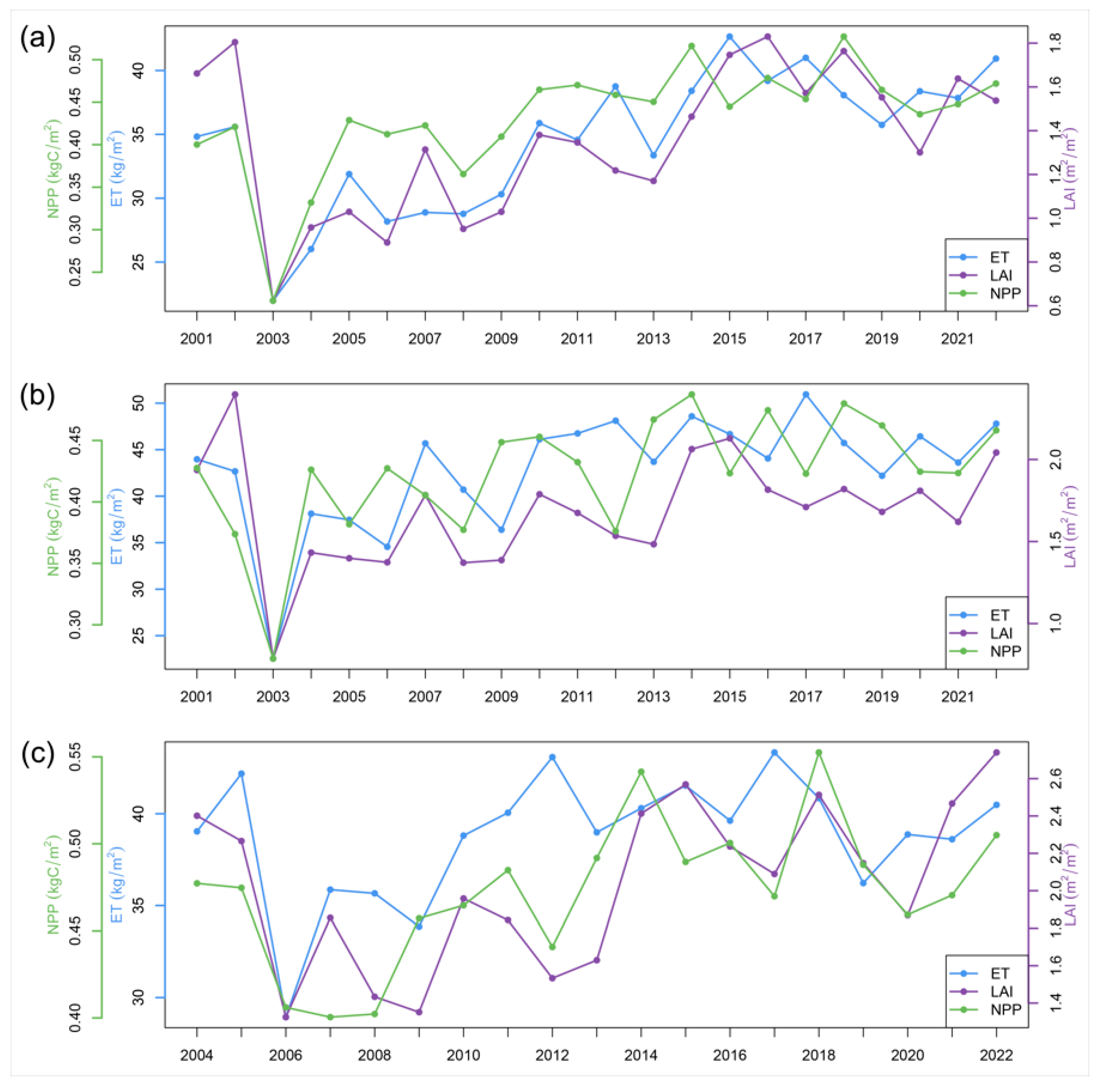
3.1. Postfire Recovery of Structural and Functional Parameters

On the basis of the MODIS product, we obtained annual observations of ecosystem states on the basis of the selected key functioning and structural parameters (i.e., NPP, ET, and LAI) (Figure 3). The overall statistics of the three fires revealed obvious differences in prefire ecosystem states, among which the GH fires had the lowest NPP, ET, and LAI values (Figure 3a). Fire disturbance caused similarly strong and rapid declines in ecosystem states for the three fires but differed substantially in magnitude, as measured by the relative proportion (see

Table 4. Statistics on the average magnitude and relative proportion of fire-induced ecosystem state changes and for three extreme fire events.

Fire Name	NPP		ET		LAI
	Magnitude	Proportion	Magnitude	Proportion	Magnitude	Proportion
GH	0.19	47%	13.23	38%	1.11	64%
Huma	0.13	32%	20.78	48%	1.34	64%
KDH	0.07	15%	11.68	29%	1.00	43%

). The postfire recovery trajectories of ecosystem states clearly revealed various responses to wildfire disturbance, either from the perspective of ecosystem states or from the perspective of fire events per se.

Although we observed pronounced interannual variability from the postfire recovery trajectories, especially for the KDH fire (Figure 3c), all ecosystem states exhibited significant positive trends but differed greatly among fires and parameters. The NPP and ET can approach prefire levels much earlier than the LAI does in most cases. For the GH and Huma fires, the mean annual NPP rapidly returned to the prefire level within 3–5 years, while the ET required 7–9 years, whereas the LAI did not approach the prefire standard within 16 years. The KDH fire, which had notably better prefire NPP and LAI states but lower ET states than the other two fires, represented faster ET recovery but slower and unstable NPP recovery, both of which require approximately 5–7 years to approach the prefire condition. The trajectory of the LAI showed remarkable interannual fluctuations, which, as a comparison, can approach the prefire standard at approximately 8–10 years, which is much earlier than the other two fires.

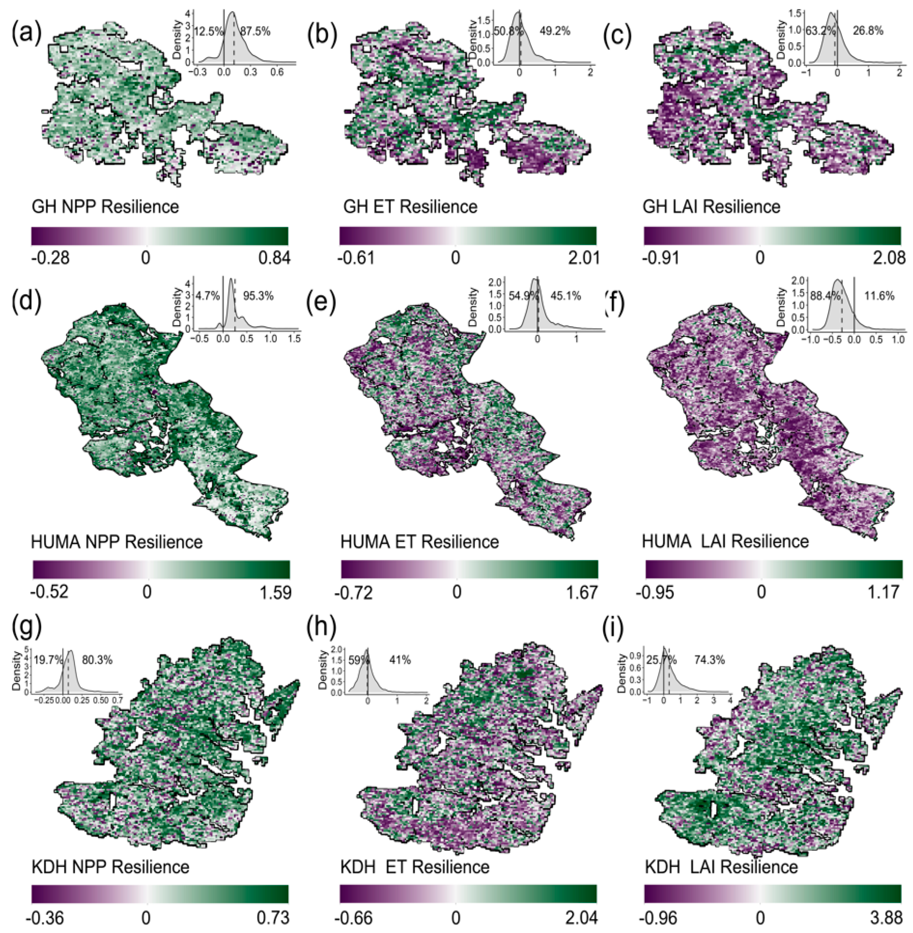
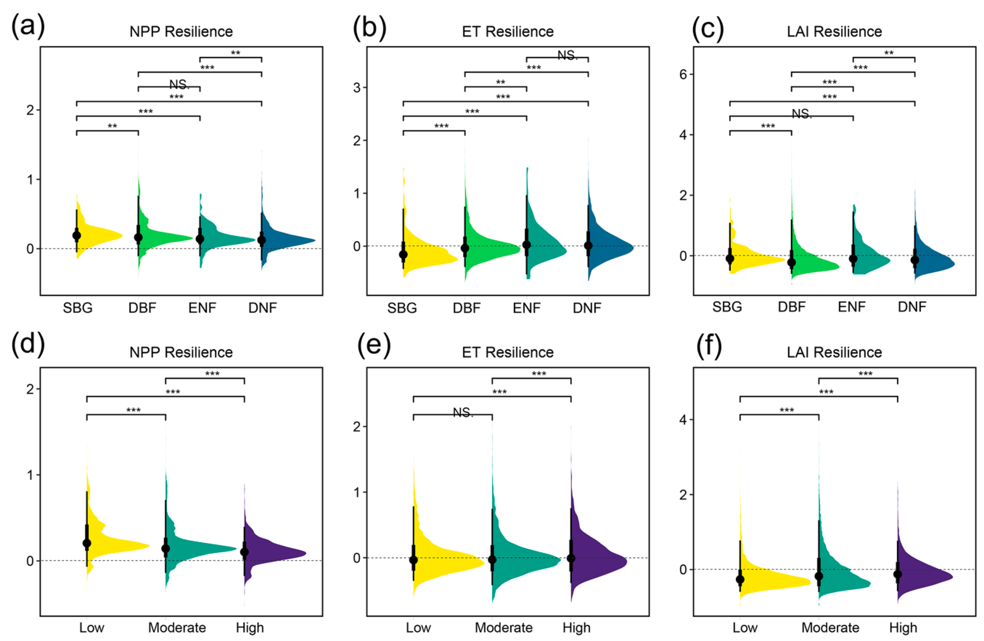
3.2. Spatial Pattern of Ecosystem Resilience

We generated wall-to-wall evaluations of forest resilience according to the time series analysis of NPP, ET, and LAI, as shown in Figure 4. The positive resilience values suggested that the ecosystem state had reached or even exceeded the prefire level, yet the negative values indicated states of partial recovery. Our results showed that resilience varied considerably among ecosystem properties. NPP exhibits superior resilience compared with the other two parameters, as more than 80% of the burned areas of three fires were evaluated with positive resilience values (Figure 4a,d,g). In contrast, at least 50% of the burned area of three fires had negative resilience values for ET. The LAI generally represented the least resilience, as shown for the GH and Huma fires (Figure 4d,f), but interestingly, we found that a relatively high proportion of the burned area (74.3%) for the KDH fire reached the prefire level (Figure 4i). Our results clearly revealed that structural and functional properties have inconsistent responses to wildfire disturbance, which implies that their resilience is regulated by complex interactions.

We used analysis of variance (ANOVA) to compare differences in resilience among groups divided by prefire vegetation types and burn severity classes for the three fires together. For vegetation type, nearly all null hypotheses were rejected at the p < 0.05 level. This indicates that the resilience values of the three ecosystem properties significantly differed between vegetation types, except for three cases (Figure 5a–c). The shrub–grassland type had the highest NPP resilience, as expected, followed by the DBF, ENF, and DNF types. There was not enough evidence to support the rejection of the null hypothesis when the NPP resilience of DBF was compared with that of ENF. In contrast, shrub–grassland and DBF had significantly weaker ET resilience than the two needle-leaved forests (i.e., ENF and DNF), whose differences were not significant. All four vegetation types exhibited negative LAI resilience, whereas shrub–grassland and ENF did not significantly differ, with slightly higher LAI resilience than DBF and DNF.

We used the RdNBR to roughly classify burned areas into three categories (i.e., low, moderate, and high) and compared their resilience accordingly. Except for the insignificant difference in ET resilience between the low- and moderate-severity classes, we observed that the resilience of the three ecosystem properties differed significantly among the three classes of burn severity (Figure 5d–f). Our results suggest that wildfires have differential impacts on the resilience of vegetation. Interestingly, we observed a stark contrast between the resilience of the LAI and NPP in different burn severity classes. While the NPP exhibited a decreasing trend with increasing severity, the LAI exhibited the opposite pattern.

3.3. GBM-SHAP Modeling for Ecosystem Resilience

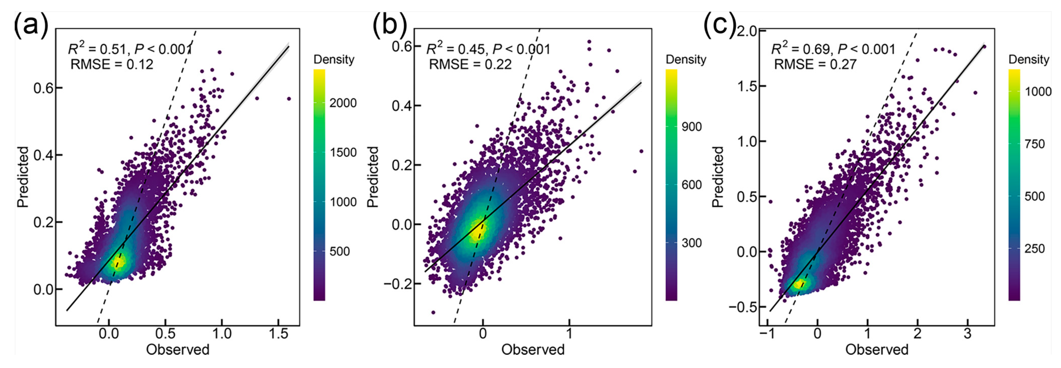
3.3.1. Model Validation and Variable Importance

We established three GBM models to illustrate the underlying mechanisms driving ecosystem resilience. We used the same sets of spatial points featuring consistent explanatory variables to train and validate these models. The three models achieved moderate-to-high goodness of fit in terms of R² and RMSE values, suggesting that the models can capture the underlying trends and variability in the data. According to the linear regression analysis shown in Figure 6, the LAI resilience model (R² = 0.69, RMSE = 0.27) outperformed the resilience models of NPP (R² = 0.51, RMSE = 0.12) and ET (R² = 0.45, RMSE = 0.22).

We used the SHAP value to evaluate the relative contribution of a given predictor variable to improve model performance when the variance in ecosystem resilience was fit. In addition to the global SHAP value (the mean absolute SHAP value) per explanatory variable (see Figure 7b,d,f), the GBM-SHAP model also generated a SHAP value for each training data point that was organized as a summary plot (see Figure 7a,c,e) to illustrate the range and distribution of impacts from the input predictors. The Trend_minpre variable of the NPP resilience model is set as an example (Figure 7a), and the summary plot shows that the higher values of this predictor decrease its SHAP values and therefore pull the prediction toward low resilience (negative). This result could be interpreted as the area with an increasing trend in the minimum monthly precipitation in the growing season (wetter in dry months), which could favor the suppression of NPP resilience.

Our results generally indicate that extreme climate-related predictors, burn severity, and elevation are important variables that play predominant roles in regulating ecosystem resilience. However, we noted that the specific importance order and variables for different ecosystem properties varied considerably. Furthermore, the prefire vegetation composition did not strongly influence the three types of resilience, as expected. For NPP, we found that two extreme precipitation-related variables, the trend of minimum precipitation (Trend_minpre) and the mean maximum precipitation (Mean_maxpre) during the growing season, especially the first, had the most important impacts on NPP resilience. The elevation and burn severity followed these two climatic variables and had negative impacts on NPP resilience. For ET, Mean_mintmp notably outperforms the other variables that regulate ET resilience, followed by elevation, Trend_maxpre, and two AI-related variables whose SHAP values differ slightly. For the LAI, Trend_mintmp has a significantly stronger impact than the other variables on regulating the LAI resilience. The burn severity was identified with certain impacts along with some extreme climate conditions.

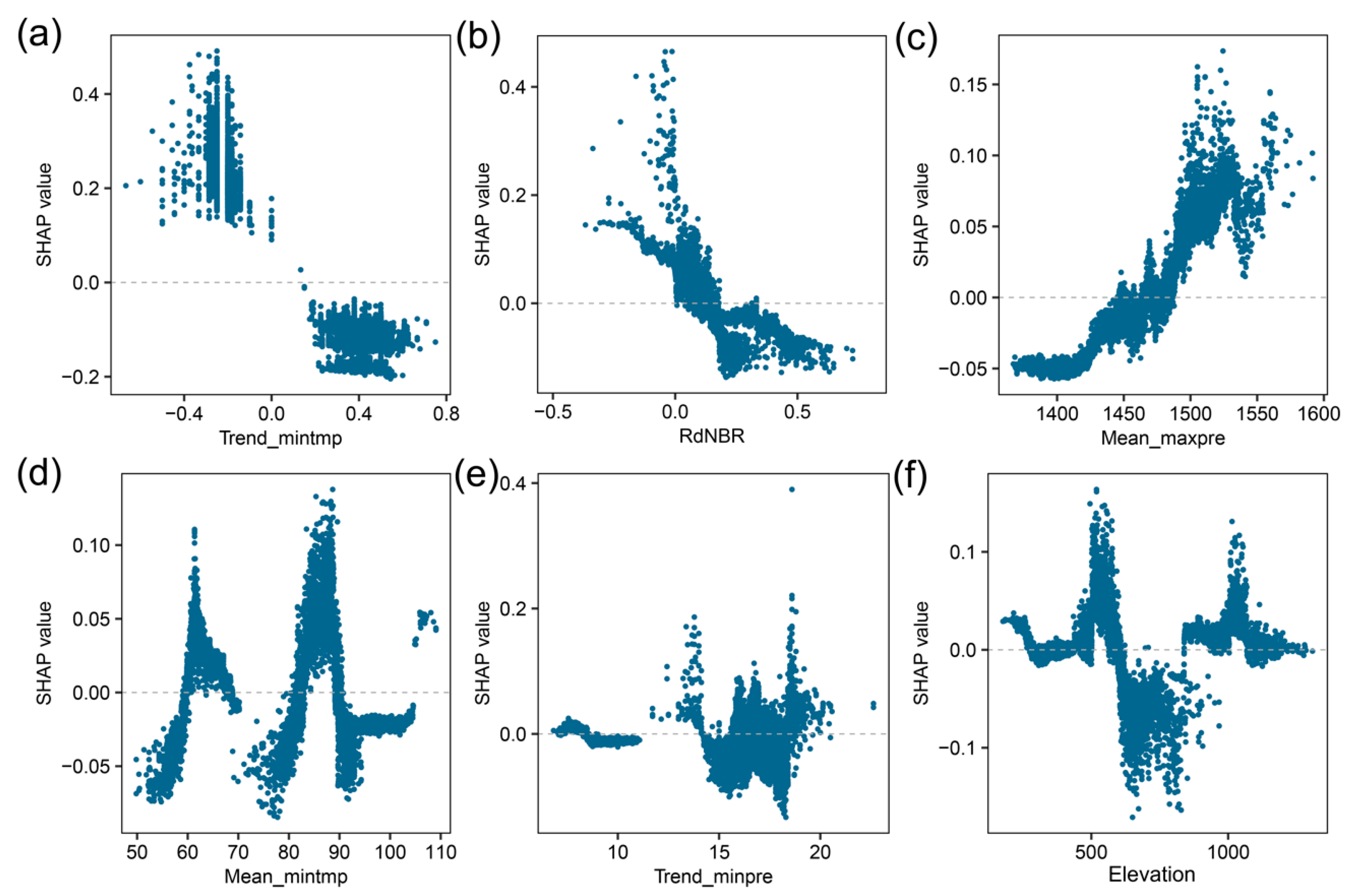
3.3.2. Explanation of Drivers Regulating Ecosystem Resilience

The partial dependence plot (PDP) approach was used to depict the response relationships between ecosystem resilience and explanatory predictors, as shown in Figure 8, Figure 9 and Figure 10. Owing to limited space and variable importance, only the top six variables ranked on the basis of the global SHAP values from the three resilience models are reported. As we described above, the GBM-SHAP model can handle nonlinear relationships between responses and predictors well. The point clouds in the PDP clearly demonstrated the potential regulatory mechanisms that drive postfire ecosystem response. It can also identify key thresholds of predictors at which the response may shift in impact magnitude or even direction.

We found that the top five variables in terms of NPP resilience exhibited negative impacts on NPP resilience. Burned areas featuring reduced trends in minimum precipitation (e.g., Trend_minpre < 11 mm/month), less monthly maximum precipitation (e.g., Mean_maxpre < 1410 mm), low minimum temperature (e.g., Mean_mintmp < 66 °F), low altitude (e.g., elevation < 400 m), and low severity (e.g., RdNBR < 0.20) favor positive NPP resilience (Figure 8).

The Mean_mintmp, DEM, and Trend_maxpre values exhibited complex fluctuations yet generally had negative relationships with ET resilience (Figure 9). The ET resilience decreased with increasing minimum temperature, maximum precipitation, and elevation. The reversed U curves for the two aridity index-derived variables suggested that ET resilience can be enhanced within certain humid environments (e.g., mean AI < 1.44). If the thresholds are overridden, the ET resilience will be eroded. The prefire coverage of DNF was found to have positive impacts on ET resilience, implying that larch forest stands favor better ET resilience.

Three variables, Trend_mintmp, RdNBR, and Mean_maxpre, clearly affected the LAI resilience (Figure 10a–c). The first two variables clearly had a negative impact, whereas the latter had a positive influence. Burned areas with a negative trend in minimum temperature tended to have enhanced LAI resilience. In contrast, areas with greater burn severity or less extreme precipitation during the growing season showed diminished LAI resilience. The other three variables, such as Mean_mintmp, Trend_minpre, and elevation, displayed bimodal or even more fluctuating curve patterns, suggesting complex interactions with other environmental factors (Figure 10d–f).

4. Discussion

It is widely recognized that LAI, NPP, and ET are closely interconnected within healthy forest ecosystems. However, our findings demonstrate that fire disturbance can disrupt or reshape these relationships, exhibiting significant spatial asynchrony in terms of their resilience. We observed that NPP is more resilient than LAI and ET, which highlights the differential responses of ecosystem processes to postfire disturbance. We believe that this reflected a prioritization of functional restoration over structural recovery in the postfire landscape of the GXM, as well as a complex allocation of resources and adaptive strategies to environmental conditions. The resources are allocated primarily toward enhancing photosynthesis and biomass accumulation rather than full canopy reestablishment. Early NPP recovery may help mitigate the negative impacts of disturbance by rapidly reestablishing carbon sinks and biomass accumulation [48], whereas the subsequent recovery of LAI and ET may support long-term structural integrity and water balance.

ET is a highly complex process, with spatial variability influenced by both vegetation characteristics (e.g., health, vigor, and vegetation type) [13,26,49,50] and regional disparities in water and thermal conditions [51,52]. Our findings revealed that the ET recovery rates of the three extreme fires were suboptimal but displayed significant spatial heterogeneity. For the GH fire, areas with good ET recovery often coincided with regions exhibiting strong recovery in NPP and LAI. However, for the other two wildfires, certain areas presented favorable NPP and LAI recoveries but experienced lower ET recovery rates, potentially attributable to differences in vegetation types. We considered that fire-induced alterations in soil properties and surface runoff [53], together with their recovery processes and interannual climate variations, determine the pattern of ET recovery. According to the analysis, the needle-leaved forests presented faster postfire recovery of ET than did the broadleaved forests and shrub–grasslands. We believe that, compared with broad leaves, ENF and DNF have smaller surface areas [54], which can reduce water loss through transpiration, especially under dry conditions. Their lower prefire ET levels can be easily restored.

We initially hypothesized that landscape-scale factors, such as prefire vegetation composition, burn severity, and topographic conditions, would exert a greater relative influence on regulating key structural and functional parameters of ecosystems than would climate-related factors. Our findings indicate that climate-related factors during the growing season, particularly trends in extreme precipitation (indicative of droughts or floods) or low-temperature events, play a more critical role in regulating the resilience of ecosystem structure and functional parameters. At the landscape scale, environmental drivers align with prior research, notably highlighting the significant role of elevation in modulating wildfire severity. In areas experiencing low-severity fires, higher survival rates of seed trees often lead to faster ecosystem recovery, suggesting greater resilience. This pattern is consistent with the established dynamics observed in the boreal forests of North America [55] and Siberia [56], as well as subalpine forest ecosystems in the western United States [10,26,57]. However, when multiple wildfires are considered, the regulatory influence of landscape-scale drivers becomes intertwined with, and in some cases dominated by, climatic factors. This complexity, often influenced by spatial variability in climate extremes, is rarely addressed or fully explored in studies focusing solely on single-fire case analyses.

According to our analysis, the increasing trend in minimum monthly precipitation during the growing season (i.e., wetter dry seasons) and the increase in maximum monthly precipitation (i.e., wetter rainy seasons) both inhibited the resilience of NPP. However, we observed that an increase in maximum precipitation during the growing season enhanced LAI resilience. This apparent paradox arises from the differing ecological processes underpinning LAI expansion and productivity accumulation. Postfire forest ecosystems often experience an increase in surface hydrophobicity, which leads to increased runoff [58,59,60]. This process results in the loss of the majority of rainfall and soil nutrients, thereby exacerbating water and nutrient limitations [61,62]. Increased precipitation alleviates water limitations, promoting rapid foliar development and increased plant density [24,63,64], leading to accelerated recovery of the LAI.

However, excessive precipitation can impose indirect constraints on productivity. Leaching of essential soil nutrients, particularly nitrogen, may occur under conditions of increased rainfall, leading to nutrient limitations that inhibit photosynthetic efficiency and carbon assimilation. An overly wet environment can reduce stomatal conductance and create hypoxic soil conditions [65], impairing root function [66,67] and slowing biomass accumulation. In addition, excessive precipitation during the growing season, along with the associated reduction in sunlight duration, can lead to decreased NPP. High LAI values may increase light attenuation within the canopy, resulting in greater self-shading and reducing the efficiency of lower canopy layers in contributing to overall productivity [25,68,69,70]. This decoupling of structural recovery (e.g., LAI) and functional recovery (e.g., NPP) underscores the nonlinear and context-dependent responses of ecosystems to hydrological changes, highlighting the complex interplay between climatic drivers and ecological processes during postfire recovery.

Nevertheless, in the management of postfire forest landscapes, greater emphasis should be placed on leveraging topographic features and prefire vegetation conditions to mitigate the legacy effects of burn severity on postfire ecosystems. After all, practical forest management interventions are predominantly implemented at the landscape scale. Our previous research suggested that integrating topography and vegetation characteristics to alter prefire fuel conditions is the most effective strategy. This approach is especially pertinent given the anticipated intensification of future wildfire regimes, where reducing fire severity may prove more critical than limiting burned area. Increasing the availability of seed sources within the landscape by increasing the presence of seed tree refugia can significantly improve the resilience of ecosystem structure and functionality. Such measures can better prepare forests to adapt to the combined effects of climate change and megafire disturbances.

We admit that several limitations may have influenced our findings. To ensure data consistency, extended temporal coverage, and reliable data availability for ecosystem change analyses, we utilized the widely employed and validated MODIS product dataset. However, potential limitations associated with the dataset’s coarse spatial resolution, sensor errors, and multispectral response issues may influence our analytical results. In our data processing, we employed the MVC approach to generate annual composites, aiming to mitigate the effects of imaging interference, which may introduce a degree of overestimation in derived indices. Furthermore, we refrained from applying any filtering or smoothing techniques to the raw data, thereby preserving data integrity but potentially increasing interannual variability in related metrics. Additionally, our findings may be subject to influences arising from inherent issues in the MODIS product generation process. For example, LAI product relies on a look-up table inversion of a 3D radiative transfer model. This approach can misrepresent canopy structure in heterogeneous landscapes, and vegetation misclassification leads to biased LAI estimates. The NPP product was derived using a light use efficiency (LUE) model, which assumes a constant maximum LUE and been adjusted by temperature and vapor pressure deficit. However, real-world LUE variability due to nutrient limitations and species composition, factors not explicitly modeled, can result in inaccurate NPP estimates in specific regions.

This research focused on three extreme wildfires in the GXM region, thereby limiting the scope of our analysis. Our study primarily focused on investigating the spatial patterns of ecosystem resilience and their driving mechanisms within the context of large-scale wildfires. While we acknowledge that smaller fires are more common within this region, as is the case in many other forest ecosystems. Due to limitations imposed by our scope, we were unable to examine the differential impacts of fire size on forest resilience in this study. This aspect, however, remains a critical consideration for both forest fire management and ecosystem recovery, and thus necessitates further investigation.

5. Conclusions

Using MODIS time series data, we analyzed the postfire evolution of key structural and functional parameters following three extreme fires in the Greater Xing’an Mountains. We identified the key factors and potential driving mechanisms that regulate the spatial patterns of postfire resilience for NPP, ET, and LAI. Our results revealed a significant spatial asynchrony of these three parameters in response to fire disturbance, with NPP exhibiting greater resilience than ET and LAI. This highlights NPP as a crucial early indicator of postfire ecological recovery, whereas LAI and ET serve as important indicators for evaluating medium- to long-term recovery quality. Our analysis indicates that, in the context of large wildfires, extreme precipitation and temperature exert a more significant influence on the regulation of these key parameters than landscape-scale factors (e.g., severity, topography, and prefire vegetation composition). This finding emphasized the importance of considering climatic factors, landscape heterogeneity and prefire conditions together in postfire recovery assessments. Moreover, the early recovery of NPP in comparison with that of LAI and ET offers critical insights into ecosystem resilience and adaptive capacity in the aftermath of fire. This emphasizes the need to prioritize functional restoration in the short term, which can lay the foundation for longer-term structural recovery and overall ecosystem resilience. This understanding provides valuable guidance for postfire management strategies, enabling the optimization of resource allocation to accelerate the restoration of ecosystem processes and services.

References

1. Mann, C.; Hernández-Morcillo, M.; Ikei, H.; Miyazaki, Y. The socioeconomic dimension of forest therapy: A contribution to human well-being and sustainable forest management. Trees For. People 2024, 18, 100731. [Google Scholar] [CrossRef]
2. Jones, M.W.; Abatzoglou, J.T.; Veraverbeke, S.; Andela, N.; Lasslop, G.; Forkel, M.; Smith, A.J.P.; Burton, C.; Betts, R.A.; van der Werf, G.R.; et al. Global and Regional Trends and Drivers of Fire Under Climate Change. Rev. Geophys. 2022, 60, e2020RG000726. [Google Scholar] [CrossRef]
3. Johnstone, J.F.; Celis, G.; Chapin III, F.S.; Hollingsworth, T.N.; Jean, M.; Mack, M.C. Factors shaping alternate successional trajectories in burned black spruce forests of Alaska. Ecosphere 2020, 11, e03129. [Google Scholar] [CrossRef]
4. Scheffer, M.; Hirota, M.; Holmgren, M.; Van Nes, E.H.; Chapin III, F.S. Thresholds for boreal biome transitions. Proc. Natl. Acad. Sci. USA 2012, 109, 21384–21389. [Google Scholar] [CrossRef] [PubMed]
5. Stevens-Rumann, C.; Morgan, P. Repeated wildfires alter forest recovery of mixed-conifer ecosystems. Ecol. Appl. Publ. Ecol. Soc. Am. 2016, 26, 1842–1853. [Google Scholar] [CrossRef]
6. Whitman, E.; Parisien, M.-A.; Thompson, D.K.; Flannigan, M.D. Topoedaphic and Forest Controls on Postfire Vegetation Assemblies Are Modified by Fire History and Burn Severity in the Northwestern Canadian Boreal Forest. Forests 2018, 9, 151. [Google Scholar] [CrossRef]
7. Baho, D.L.; Allen, C.R.; Garmestani, A.S.; Fried-Petersen, H.B.; Renes, S.E.; Gunderson, L.H.; Angeler, D.G. A quantitative framework for assessing ecological resilience. Ecol. Soc. J. Integr. Sci. Resil. Sustain. 2017, 22, 1–17. [Google Scholar] [CrossRef]
8. Sasaki, T.; Furukawa, T.; Iwasaki, Y.; Seto, M.; Mori, A.S. Perspectives for ecosystem management based on ecosystem resilience and ecological thresholds against multiple and stochastic disturbances. Ecol. Indic. 2015, 57, 395–408. [Google Scholar] [CrossRef]
9. Holling, C.S. Resilience and Stability of Ecological Systems. Annu. Rev. Ecol. Syst. 1973, 4, 1–23. [Google Scholar] [CrossRef]
10. Higuera, P.E.; Metcalf, A.L.; Miller, C.; Buma, B.; McWethy, D.B.; Metcalf, E.C.; Ratajczak, Z.; Nelson, C.R.; Chaffin, B.C.; Stedman, R.C.; et al. Integrating Subjective and Objective Dimensions of Resilience in Fire-Prone Landscapes. Bioscience 2019, 69, 379–388. [Google Scholar] [CrossRef]
11. Seidl, R.; Fernandes, P.M.; Fonseca, T.F.; Gillet, F.; Jönsson, A.M.; Merganičová, K.; Netherer, S.; Arpaci, A.; Bontemps, J.-D.; Bugmann, H.; et al. Modelling natural disturbances in forest ecosystems: A review. Ecol. Model. 2011, 222, 903–924. [Google Scholar] [CrossRef]
12. Seidl, R.; Thom, D.; Kautz, M.; Martin-Benito, D.; Peltoniemi, M.; Vacchiano, G.; Wild, J.; Ascoli, D.; Petr, M.; Honkaniemi, J.; et al. Forest disturbances under climate change. Nat. Clim. Chang. 2017, 7, 395–402. [Google Scholar] [CrossRef]
13. Turner, M.G. Disturbance and landscape dynamics in a changing world. Ecology 2010, 91, 2833–2849. [Google Scholar] [CrossRef] [PubMed]
14. Folke, C.; Carpenter, S.R.; Walker, B.; Scheffer, M.; Chapin, T.; Rockström, J. Resilience Thinking: Integrating Resilience, Adaptability and Transformability. Ecol. Soc. 2010, 15, 20. [Google Scholar] [CrossRef]
15. Cumming, G.S.; Barnes, G.; Perz, S.; Schmink, M.; Sieving, K.E.; Southworth, J.; Binford, M.; Holt, R.D.; Stickler, C.; Van Holt, T. An Exploratory Framework for the Empirical Measurement of Resilience. Ecosystems 2005, 8, 975–987. [Google Scholar] [CrossRef]
16. Yi, C.; Jackson, N. A review of measuring ecosystem resilience to disturbance. Environ. Res. Lett. 2021, 16, 053008. [Google Scholar] [CrossRef]
17. Stephens, S.L.; Collins, B.M.; Fettig, C.J.; Finney, M.A.; Hoffman, C.M.; Knapp, E.E.; North, M.P.; Safford, H.; Wayman, R.B. Drought, Tree Mortality, and Wildfire in Forests Adapted to Frequent Fire. BioScience 2018, 68, 77–88. [Google Scholar] [CrossRef]
18. Stevens-Rumann, C.S.; Kemp, K.B.; Higuera, P.E.; Harvey, B.J.; Rother, M.T.; Donato, D.C.; Morgan, P.; Veblen, T.T. Evidence for declining forest resilience to wildfires under climate change. Ecol. Lett. 2018, 21, 243–252. [Google Scholar] [CrossRef]
19. North, M.P.; Tompkins, R.E.; Bernal, A.A.; Collins, B.M.; Stephens, S.L.; York, R.A. Operational resilience in western US frequent-fire forests. For. Ecol. Manag. 2022, 507, 120004. [Google Scholar] [CrossRef]
20. Fernandez-Manso, A.; Quintano, C.; Roberts, D.A. Burn severity influence on postfire vegetation cover resilience from Landsat MESMA fraction images time series in Mediterranean forest ecosystems. Remote Sens. Environ. 2016, 184, 112–123. [Google Scholar] [CrossRef]
21. João, T.; João, G.; Bruno, M.; João, H. Indicator-based assessment of postfire recovery dynamics using satellite NDVI time-series. Ecol. Indic. 2018, 89, 199–212. [Google Scholar] [CrossRef]
22. Parks, S.A.; Holsinger, L.M.; Panunto, M.H.; Jolly, W.M.; Dobrowski, S.Z.; Dillon, G.K. High-severity fire: Evaluating its key drivers and mapping its probability across western US forests. Environ. Res. Lett. 2018, 13, 044037. [Google Scholar] [CrossRef]
23. Spasojevic, M.J.; Bahlai, C.A.; Bradley, B.A.; Butterfield, B.J.; Tuanmu, M.-N.; Sistla, S.; Wiederholt, R.; Suding, K.N. Scaling up the diversity–resilience relationship with trait databases and remote sensing data: The recovery of productivity after wildfire. Glob. Chang. Biol. 2016, 22, 1421–1432. [Google Scholar] [CrossRef] [PubMed]
24. Löf, M.; Madsen, P.; Metslaid, M.; Witzell, J.; Jacobs, D.F. Restoring forests: Regeneration and ecosystem function for the future. New For. 2019, 50, 139–151. [Google Scholar] [CrossRef]
25. Seidl, R.; Turner, M.G. Post-disturbance reorganization of forest ecosystems in a changing world. Proc. Natl. Acad. Sci. USA 2022, 119, e2202190119. [Google Scholar] [CrossRef]
26. Harvey, B.J.; Donato, D.C.; Turner, M.G. High and dry: Postfire tree seedling establishment in subalpine forests decreases with postfire drought and large stand-replacing burn patches. Glob. Ecol. Biogeogr. 2016, 25, 655–669. [Google Scholar] [CrossRef]
27. Lipoma, L.; Kambach, S.; Díaz, S.; Sabatini, F.M.; Damasceno, G.; Kattge, J.; Wirth, C.; Abella, S.R.; Beierkuhnlein, C.; Belote, T.R.; et al. No general support for functional diversity enhancing resilience across terrestrial plant communities. Glob. Ecol. Biogeogr. 2024, 33, e13895. [Google Scholar] [CrossRef]
28. Lausch, A.; Erasmi, S.; King, D.J.; Magdon, P.; Heurich, M. Understanding Forest Health with Remote Sensing-Part II—A Review of Approaches and Data Models. Remote Sens. 2017, 9, 129. [Google Scholar] [CrossRef]
29. Pretzsch, H.; del Río, M.; Biber, P.; Arcangeli, C.; Bielak, K.; Brang, P.; Dudzinska, M.; Forrester, D.I.; Klädtke, J.; Kohnle, U.; et al. Maintenance of long-term experiments for unique insights into forest growth dynamics and trends: Review and perspectives. Eur. J. For. Res. 2019, 138, 165–185. [Google Scholar] [CrossRef]
30. Mandl, L.; Viana-Soto, A.; Seidl, R.; Stritih, A.; Senf, C. Unmixing-based forest recovery indicators for predicting long-term recovery success. Remote Sens. Environ. 2024, 308, 114194. [Google Scholar] [CrossRef]
31. Zhu, Z.; Zhang, J.; Yang, Z.; Aljaddani, A.H.; Cohen, W.B.; Qiu, S.; Zhou, C. Continuous monitoring of land disturbance based on Landsat time series. Remote Sens. Environ. 2020, 238, 111116. [Google Scholar] [CrossRef]
32. Fang, L.; Yang, J.; Zu, J.; Li, G.; Zhang, J. Quantifying influences and relative importance of fire weather, topography, and vegetation on fire size and fire severity in a Chinese boreal forest landscape. For. Ecol. Manag. 2015, 356, 2–12. [Google Scholar] [CrossRef]
33. Qi, Y.; Li, F. Remote Sensing Estimation of Aboveground Forest Carbon Storage in Daxing’an Mountains Based on KNN Method. Sci. Silvae Sin. 2015, 51, 46–55. [Google Scholar]
34. Wang, C.; Gower, S.T.; Wang, Y.; Zhao, H.; Yan, P.; Lamberty, B.P. The influence of fire on carbon distribution and net primary production of boreal larix gmelinii forests in north-eastern China. Glob. Chang. Biol. 2001, 7, 719–730. [Google Scholar] [CrossRef]
35. Cai, W.; Yang, J. High-severity fire reduces early successional boreal larch forest aboveground productivity by shifting stand density in north-eastern China. Int. J. Wildland Fire 2016, 25, 861–875. [Google Scholar] [CrossRef]
36. Fang, L.; Yang, J. Atmospheric effects on the performance and threshold extrapolation of multi-temporal Landsat derived dNBR for burn severity assessment. Int. J. Appl. Earth Obs. Geoinf. 2014, 33, 10–20. [Google Scholar] [CrossRef]
37. Fang, L.; Yang, J.; Zhang, W.; Zhang, W.; Yan, Q. Combining allometry and landsat-derived disturbance history to estimate tree biomass in subtropical planted forests. Remote Sens. Environ. 2019, 235, 111423. [Google Scholar] [CrossRef]
38. Stukel, M.R.; Décima, M.; Kelly, T.B.; Landry, M.R.; Nodder, S.D.; Ohman, M.D.; Selph, K.E.; Yingling, N. Relationships Between Plankton Size Spectra, Net Primary Production, and the Biological Carbon Pump. Glob. Biogeochem. Cycles 2024, 38, e2023GB007994. [Google Scholar] [CrossRef]
39. Kool, D.; Agam, N.; Lazarovitch, N.; Heitman, J.L.; Sauer, T.J.; Ben-Gal, A. A review of approaches for evapotranspiration partitioning. Agric. For. Meteorol. 2014, 184, 56–70. [Google Scholar] [CrossRef]
40. Zhang, X.; Liu, L.; Chen, X.; Gao, Y.; Xie, S.; Mi, J. GLC_FCS30: Global land-cover product with fine classification system at 30 m using time-series Landsat imagery. Earth Syst. Sci. Data 2021, 13, 2753–2776. [Google Scholar] [CrossRef]
41. Fang, L.; Crocker, E.V.; Yang, J.; Yan, Y.; Yang, Y.; Liu, Z. Competition and Burn Severity Determine Postfire Sapling Recovery in a Nationally Protected Boreal Forest of China: An Analysis from Very High-Resolution Satellite Imagery. Remote Sens. 2019, 11, 603. [Google Scholar] [CrossRef]
42. van Wagtendonk, J.W.; Root, R.R.; Key, C.H. Comparison of AVIRIS and Landsat ETM+ detection capabilities for burn severity. Remote Sens. Environ. 2004, 92, 397–408. [Google Scholar] [CrossRef]
43. Miller, J.D.; Knapp, E.E.; Key, C.H.; Skinner, C.N.; Isbell, C.J.; Creasy, R.M.; Sherlock, J.W. Calibration and validation of the relative differenced Normalized Burn Ratio (RdNBR) to three measures of fire severity in the Sierra Nevada and Klamath Mountains, California, USA. Remote Sens. Environ. 2009, 113, 645–656. [Google Scholar] [CrossRef]
44. Soverel, N.O.; Perrakis, D.D.B.; Coops, N.C. Estimating burn severity from Landsat dNBR and RdNBR indices across western Canada. Remote Sens. Environ. 2010, 114, 1896–1909. [Google Scholar] [CrossRef]
45. Elith, J.; Leathwick, J.R.; Hastie, T. A working guide to boosted regression trees. J. Anim. Ecol. 2008, 77, 802–813. [Google Scholar] [CrossRef]
46. Friedman, J.H. Greedy function approximation: A gradient boosting machine. Ann. Stat. 2001, 29, 1189–1232. [Google Scholar] [CrossRef]
47. Lundberg, S.M.; Lee, S.I. A unified approach to interpreting model predictions. Adv. Neural Inf. Process. Syst. 2017, 30, 4768–4777. [Google Scholar]
48. Mndela, M.; Tjelele, J.T.; Madakadze, I.C.; Mangwane, M.; Samuels, I.M.; Muller, F.; Pule, H.T. A global meta-analysis of woody plant responses to elevated CO2: Implications on biomass, growth, leaf N content, photosynthesis and water relations. Ecol. Process. 2022, 11, 52. [Google Scholar] [CrossRef]
49. Li, X.; Gentine, P.; Lin, C.; Zhou, S.; Sun, Z.; Zheng, Y.; Liu, J.; Zheng, C. A simple and objective method to partition evapotranspiration into transpiration and evaporation at eddy-covariance sites. Agric. For. Meteorol. 2019, 265, 171–182. [Google Scholar] [CrossRef]
50. Turner, M.G.; Chapin, F.S. Causes and Consequences of Spatial Heterogeneity in Ecosystem Function. In Ecosystem Function in Heterogeneous Landscapes; Springer: Berlin/Heidelberg, Germany, 2005; pp. 9–30. [Google Scholar]
51. Han, D.; Wang, G.; Liu, T.; Xue, B.-L.; Kuczera, G.; Xu, X. Hydroclimatic response of evapotranspiration partitioning to prolonged droughts in semiarid grassland. J. Hydrol. 2018, 563, 766–777. [Google Scholar] [CrossRef]
52. Lin, H.; Chen, Y.; Zhang, H.; Fu, P.; Fan, Z. Stronger cooling effects of transpiration and leaf physical traits of plants from a hot dry habitat than from a hot wet habitat. Funct. Ecol. 2017, 31, 2202–2211. [Google Scholar] [CrossRef]
53. Carrà, B.G.; Bombino, G.; Denisi, P.; Plaza-Àlvarez, P.A.; Lucas-Borja, M.E.; Zema, D.A. Water Infiltration after Prescribed Fire and Soil Mulching with Fern in Mediterranean Forests. Hydrology 2021, 8, 95. [Google Scholar] [CrossRef]
54. Littell, J.S.; Peterson, D.L.; Riley, K.L.; Liu, Y.; Luce, C.H. A review of the relationships between drought and forest fire in the United States. Glob. Chang. Biol. 2016, 22, 2353–2369. [Google Scholar] [CrossRef] [PubMed]
55. Balch, J.K.; Iglesias, V.; Mahood, A.L.; Cook, M.C.; Amaral, C.; DeCastro, A.; Leyk, S.; McIntosh, T.L.; Nagy, R.C.; St Denis, L.; et al. The fastest-growing and most destructive fires in the US (2001 to 2020). Science 2024, 386, 425–431. [Google Scholar] [CrossRef] [PubMed]
56. Kharuk, V.I.; Ponomarev, E.I.; Ivanova, G.A.; Dvinskaya, M.L.; Coogan, S.C.P.; Flannigan, M.D. Wildfires in the Siberian taiga. Ambio 2021, 50, 1953–1974. [Google Scholar] [CrossRef]
57. Harvey, B.J.; Donato, D.C.; Turner, M.G. Burn me twice, shame on who? Interactions between successive forest fires across a temperate mountain region. Ecology 2016, 97, 2272–2282. [Google Scholar] [CrossRef]
58. Chen, J.; McGuire, K.J.; Stewart, R.D. Effect of soil water-repellent layer depth on post-wildfire hydrological processes. Hydrol. Process. 2020, 34, 270–283. [Google Scholar] [CrossRef]
59. Vieira, D.C.S.; Malvar, M.C.; Martins, M.A.S.; Serpa, D.; Keizer, J.J. Key factors controlling the postfire hydrological and erosive response at micro-plot scale in a recently burned Mediterranean forest. Geomorphology 2018, 319, 161–173. [Google Scholar] [CrossRef]
60. Weatherholt, J.A.; Johnson, B.G. Evaluating the occurrence and spatial patterns of soil water repellency in the Deschutes National Forest, Oregon. Soil Sci. Soc. Am. J. 2024, 88, 1014–1026. [Google Scholar] [CrossRef]
61. Gustine, R.N.; Hanan, E.J.; Robichaud, P.R.; Elliot, W.J. From burned slopes to streams: How wildfire affects nitrogen cycling and retention in forests and fire-prone watersheds. Biogeochemistry 2022, 157, 51–68. [Google Scholar] [CrossRef]
62. Smith, H.G.; Sheridan, G.J.; Lane, P.N.J.; Nyman, P.; Haydon, S. Wildfire effects on water quality in forest catchments: A review with implications for water supply. J. Hydrol. 2011, 396, 170–192. [Google Scholar] [CrossRef]
63. Liu, X.; Jiao, L.; Cheng, D.; Liu, J.; Li, Z.; Li, Z.; Wang, C.; He, X.; Cao, Y.; Gao, G. Light thinning effectively improves forest soil water replenishment in water-limited areas: Observational evidence from Robinia pseudoacacia plantations on the Loess Plateau, China. J. Hydrol. 2024, 637, 131408. [Google Scholar] [CrossRef]
64. Sun, S.-S.; Liu, X.-P.; Zhao, X.-Y.; Medina-Roldánd, E.; He, Y.-H.; Lv, P.; Hu, H.-J. Annual Herbaceous Plants Exhibit Altered Morphological Traits in Response to Altered Precipitation and Drought Patterns in Semiarid Sandy Grassland, Northern China. Front. Plant Sci. 2022, 13, 756950. [Google Scholar] [CrossRef]
65. Lawson, T.; Vialet-Chabrand, S. Speedy stomata, photosynthesis and plant water use efficiency. New Phytol. 2019, 221, 93–98. [Google Scholar] [CrossRef] [PubMed]
66. Carminati, A.; Javaux, M. Soil Rather Than Xylem Vulnerability Controls Stomatal Response to Drought. Trends Plant Sci. 2020, 25, 868–880. [Google Scholar] [CrossRef]
67. Smith, D.M.; Inman-Bamber, N.G.; Thorburn, P.J. Growth and function of the sugarcane root system. Field Crops Res. 2005, 92, 169–183. [Google Scholar] [CrossRef]
68. Béland, M.; Baldocchi, D.D. Vertical structure heterogeneity in broadleaf forests: Effects on light interception and canopy photosynthesis. Agric. For. Meteorol. 2021, 307, 108525. [Google Scholar] [CrossRef]
69. Sercu, B.K.; Baeten, L.; van Coillie, F.; Martel, A.; Lens, L.; Verheyen, K.; Bonte, D. How tree species identity and diversity affect light transmittance to the understory in mature temperate forests. Ecol. Evol 2017, 7, 10861–10870. [Google Scholar] [CrossRef]
70. Tanioka, Y.; Ida, H.; Hirota, M. Relationship between Canopy Structure and Community Structure of the Understory Trees in a Beech Forest in Japan. Forests 2022, 13, 494. [Google Scholar] [CrossRef]
Figure 1. Location of the Great Xing’an Mountains (a) in Northeastern China. Three Landsat-derived relative differenced normalized burn ratio (RdNBR) images represent the burn severity patterns of three extreme fire events: the Genhe Fire (b), the Huma Fire (c), and the Kanduhe Fire (d). The RdNBR was used to quantify postfire ecosystem changes (see bd). Higher RdNBR values represent higher burn severity.
Fire 08 00108 g001
Figure 2. Forest resilience to wildfire disturbance through a time series of ecosystem state’s variable changes (modified from Yi et al. (2021) [16]). The curve illustrates the ecosystem state dynamics at three different phases, i.e., prefire, immediate postfire, and postfire recovery, which provides a visual representation of the transition from prefire stability through disturbance and subsequent recovery or reorganization.
Fire 08 00108 g002
Figure 3. Interannual variation in the mean NPP, ET, and LAI for burned areas for the GH fire (a), Huma fire (b), and KDH fire (c) cases. We rescaled the y-axis to generate a consistent and straightforward comparison between ecosystem states.
Fire 08 00108 g003
Figure 4. Map of the spatial distribution of ecosystem resilience derived from MODIS observations of structural and functional parameters for the GH (ac), Huma (df), and KDH (gi) fires. The probability density function plots in gray show the distributions of the resilience values of NPP (a,d,g), ET (b,e,h), and LAI (c,f,i). The dashed lines represent the mean values of the evaluated resilience.
Fire 08 00108 g004
Figure 5. Raincloud plots combined with ANOVA to compare the differences in NPP resilience (a,d), ET resilience (b,e), and LAI resilience (c,f) according to prefire vegetation composition, and burn severity level. The vegetation types were classified as deciduous broadleaved forest (DBF), deciduous needle-leaved forest (DNF), evergreen needle-leaved forest (ENF) and shrub–grassland (SBG). Burn severity was classified into low, moderate or high levels according to the RdNBR thresholds derived from the Jenks natural breaks algorithm. *** denotes a significant difference at the p < 0.001 level, ** denotes a significant difference at the p < 0.01 level, and NS denotes non-significance.
Fire 08 00108 g005
Figure 6. Density scatter plot of the goodness of fit between the evaluated resilience (observed) and model predictions (predicted) for NPP (a), ET (b), and LAI (c). The dashed lines represent the regression lines between the observed and predicted values, whereas the solid lines represent the 1:1 reference line.
Fire 08 00108 g006
Figure 7. SHAP summary plots representing the range and distribution of impacts of explanatory variables on NPP (a), ET (c), and LAI (e). The bar plots show the global relative contribution of explanatory variables calculated from the mean absolute SHAP value for the corresponding ecosystem states, i.e., NPP (b), ET (d), and LAI (f).
Fire 08 00108 g007
Figure 8. Partial dependence plots showing the nonlinear effects of the top six most important explanatory variables on NPP resilience prediction, namely Trend_minpre (a), Mean_maxpre (b), Elevation (c), RdNBR (d), Mean_mintmp (e), and PRE_SMK_SLOPE (f) A positive SHAP value means that the variable increases the predicted outcome, whereas a negative value indicates that the variable decreases the outcome. Please see Table 3 for a detailed explanation of the variables.
Fire 08 00108 g008
Figure 9. Partial dependence plots representing the nonlinear effects of the top six most important explanatory variables on ET resilience prediction, namely Mean_mintmp (a), Elevation (b), Trend_maxpre (c), Mean_AI (d), Max_AI (e), and DNF (f). A positive SHAP value means that the variable increases the predicted outcome, whereas a negative value indicates that the variable decreases the outcome. Please see Table 3 for a detailed explanation of the variables.
Fire 08 00108 g009
Figure 10. Partial dependence plots representing the nonlinear effects of the top six most important explanatory variables on LAI resilience prediction, namely Trend_mintmp (a), RdNBR (b), Mean_maxpre (c), Mean_mintmp (d), Trend_minpre (e), and Elevation (f). A positive SHAP value means that the variable increases the predicted outcome, whereas a negative value indicates that the variable decreases the outcome. Please see Table 3 for a detailed explanation of the variables.
Fire 08 00108 g010