Abstract
In cold regions, fire pipes are highly susceptible to freezing, which can obstruct water flow and lead to pipe ruptures. Accurately predicting the freeze thickness is crucial to maintaining the functionality of fire protection systems. Traditional methods for predicting fire pipe freezing often rely on simplified models or time-consuming simulations, which limits their accuracy in complex environments. A model for predicting the freeze thickness of fire pipes under low-temperature conditions was developed by integrating Computational Fluid Dynamics with an Artificial Neural Network (ANN). The CFD model was validated to generate data for training and optimizing an ANN based on collected experimental data. The CFD results demonstrate a nonlinear relationship between the freeze thickness of the fire pipe, ambient temperature, and time. Afterwards, the optimal ANN topology, determined through hyperparameter tuning, was found to consist of 12 neurons, the trainlm training function, and tansig–purelin activation functions. Eventually, the ANN model achieved high prediction accuracy with a mean squared error (MSE) of 6.62 × 10⁻⁴ on the test set and a regression coefficient R greater than 0.98 across all datasets. Furthermore, the ANN model agrees closely with the simulated data, not only for trained temperature conditions (−5 °C to −50 °C) but also for unseen temperature conditions (−55 °C and −60 °C), indicating excellent generalization performance.
1. Introduction
With the acceleration of urbanization and the continuous refinement of building safety standards, ensuring the reliability of fire protection systems has become crucial for guaranteeing public safety [1,2]. Fire pipes, which represent key components of these systems, play a critical role in enabling timely and effective firefighting operations during fires [3,4]. However, in regions with cold or extreme weather conditions, fire pipes experience severe freezing risks. When the water within these pipes freezes, it can not only disrupt normal water flow but also lead to pipe ruptures in severe cases, causing substantial economic losses and posing serious safety hazards [5,6]. Hence, examining and predicting the freezing process in fire pipes under low-temperature conditions is essential for establishing effective antifreeze measures, optimizing pipe design, and boosting the overall reliability of fire protection systems.
Previous studies have attempted to address this issue. For instance, Park et al. [7] numerically analyzed the icing process within an externally exposed U-shaped pipe by considering the mushy region of ice formation. Kim et al. [8] investigated the antifreeze effects of heating wires through numerical simulations. While these approaches offer some theoretical foundation for preventing fire pipe freezing, most traditional freezing prediction methods typically rely on simplified models or time-consuming computational fluid dynamics (CFD) simulations [9,10,11,12]. Although these simulations offer a certain level of accuracy, they require considerable computational resources, particularly when addressing the complexities of real-world environments. Furthermore, the limitations in accounting for nonlinear factors in such environments often result in suboptimal prediction accuracy [13,14]. These issues pose challenges for reliable cryogenic pipe freezing predictions in complex environments.
In recent years, the rapid advancements in artificial intelligence technology, particularly in the field of machine learning (ML), have fueled the development of novel approaches for predicting the freezing processes occurring within fire pipes, thus helping to overcome the limitations of traditional methods [15,16,17,18]. Compared to traditional CFD simulations, ML techniques can more efficiently capture the complex relationships between inputs and outputs by learning from extensive datasets, thereby offering faster and more precise predictions. This advantage is particularly evident when dealing with dynamic, nonlinear, and complex systems.
Among the most promising ML techniques is the artificial neural network (ANN), known for its ability to handle complex system prediction problems due to its powerful nonlinear mapping capabilities, self-learning features, and adaptability [19,20]. By training on large datasets, ANNs can effectively model the intricate relationships between input variables (e.g., environmental temperature, pipe material, and freezing duration) and output variables (e.g., freezing thickness), enabling accurate predictions. Multi-objective optimization using ANNs and genetic algorithms, as demonstrated by Salakhi et al. [21], is one example of how these networks can be leveraged for optimal design in similar contexts. Furthermore, Khaboshan et al. [22]. explored the potential of artificial intelligence, combined with CFD, to predict the average battery surface temperature and liquid fraction of phase-change materials. This potential has been further exemplified by Cho et al. [16], who used outdoor fire pipe data to train several ML algorithms—including deep neural networks, decision trees, random forests, and support vector machines—to predict the temperature of freeze protection systems for metal heaters. However, most existing ML-based studies have predominantly focused on predicting temperature distributions, largely overlooking the direct freezing process itself.
To address this gap, the present study integrates CFD and the ANN to develop a predictive model for freeze thicknesses in fire pipes subjected to low-temperature environments. A numerical CFD model was first constructed and validated with experimental data generated via simulations. These results not only served to verify the CFD model’s accuracy but also provided the necessary training data for the ANN model. The ANN was then designed and optimized to predict the freezing thickness of fire pipes under varying ambient temperatures and time intervals. The novelty of this work lies in its focus on freeze thickness prediction, an area that has been underexplored in ML studies related to freeze protection systems.
In summary, the proposed prediction method, combining the CFD and ANN techniques, is intended to offer a new technical approach for designing and optimizing fire pipes to prevent freezing under low-temperature conditions. The findings of this study are anticipated to help boost the reliability and safety of fire protection systems in regions with cold or extreme weather conditions. Furthermore, the proposed method is expected to find applications in other engineering domains involving low-temperature freezing processes, such as hydropower pipelines and water supply systems, demonstrating notable theoretical significance and practical application value.
2. Methods
2.1. Experimental Setup
The experimental data for this study were sourced from the literature [23]. The test system comprised refrigeration equipment, an insulation box, a fire pipe, a ventilation system, and a temperature monitoring system, as shown in Figure 1a. The fire pipe utilized in the experiment was a 1 m seamless steel pipe with a DN150 diameter, connected to flanges on both sides. A T-type thermocouple was connected to a data acquisition instrument (Keithley DAQ6510, Tektronix Inc., Shanghai, China) outside the system, which recorded real-time data on the ambient air temperature, fire pipe wall temperature, and water temperature. During the test, temperature measurement points were set at 1/3 and 2/3 of the length of the fire pipe’s outer wall, as shown in Figure 1b. The experiment was conducted under three temperature conditions: −12.8 °C, −10 °C, and −7 °C.
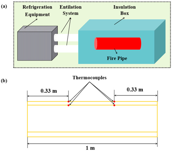
Figure 1.
The schematic diagram of the experimental system (a) and fire pipe (b): Yellow lines: pipe front view. Arrows: The identifier. Red dots: Thermocouples.
2.2. Basic Numerical Simulation Setup
Numerical modeling of the fire pipe (DN150) was conducted using CFD software (Fluent 2023) [24], as illustrated in Figure 2. The fire pipe is modeled only in the cross-sectional plane, rather than as a full 3D structure. This simplification was made to focus on the key aspects of the freezing process while reducing computational complexity. The initial ambient temperature was 5 °C. The pipe featured an inner diameter of 150 mm and an outer diameter of 169 mm. Meshing was performed using quadrilateral elements, and the simulation results for mesh sizes of 1 mm and 2 mm were compared. Table 1 outlines the primary properties of each material used in the simulation analysis, predominantly focusing on the variations in the thermal conductivities of water and ice while disregarding changes in density and heat capacity. To monitor temperature changes and phase transitions during the simulation, a thermocouple and a liquid fraction sensor were strategically positioned on the inner surface of the pipe wall, enabling precise temperature measurements at key locations.
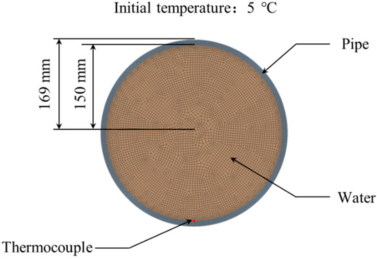
Figure 2.
Modeling schematic of the parts, dimensions, and measurement positions for CFD analysis.

Table 1.
Material Properties [25].
The numerical simulation process follows the conservation of mass and momentum. Based on the theory of transient heat conduction, whatever the shape of the model can be analyzed according to the type of heat transfer, and the control equation is:
where kx, ky, and kz are the thermal conductivity of x, y, and z (W/m·K); q is the heat growth rate (W/m3); ρ is the density (kg/m3); and c is the specific heat capacity (J/kg·K).
The solidification/melting process is modeled using the enthalpy-porosity technique in ANSYS Fluent 2023. In this technique, a quantity called the liquid fraction (the fraction representing the liquid volume) is associated with each unit in the domain. Based on enthalpy equilibrium, the liquid fraction is calculated at each iteration. The paste region is the region where the liquid fraction is between 0 and 1. The paste region is modeled as a “pseudo-” porous medium in which porosity decreases from 1 to 0 as the material solidifies. For more information on this method, see the work of Voller and Prakash et al. [26]. A series of liquid fraction measuring points are arranged in the direction of pipe diameter to measure the freeze thickness during a temperature drop.
2.3. Model Verification
In a previous study, Kim et al. [8] utilized mesh sizes of 2 mm, 2.5 mm, and 3 mm. Table 2 illustrates the results of the grid independence and time step analysis of the numerical simulation, showing the start freezing time for different grid sizes and time step intervals. It is apparent from this table that NO-II with 17,671 cells and 100 s time-step are appropriate for this study.
Table 2.
Investigation of start freezing time at −10 °C.
Notably, heat transfer within the experimental system primarily occurs through radiation, conduction, and convection. Among these, radiative heat transfer is primarily determined by temperature and shape, conductive heat transfer is governed by thermal conductivity, and convective heat transfer is largely influenced by the convective heat transfer coefficient. For the circular fire pipe considered in this study, temperature changes directly influence radiative heat transfer calculations, while thermal conductivity remains constant. Meanwhile, the convective heat transfer coefficient requires additional calculations to account for the temperature changes. Previous studies have examined the convective heat transfer coefficients of circular pipes, revealing that the following relationship exists between the convective heat transfer coefficient (h) and the temperature difference (ΔT):
where a and b denote constants, respectively [27,28]. The experimental data corresponding to temperatures of −12.8 °C, −10 °C, and −7 °C were verified through a trial-and-error approach, and the results are displayed in Figure 3. Next, the relationship between the convective heat transfer coefficient and temperature difference was fitted (Figure 4) based on the aforementioned three simulation results using the following equation:
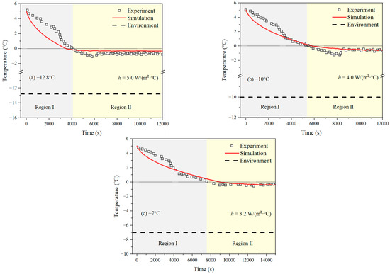
Figure 3.
Comparison of experimental data with simulation results at different temperatures to determine the convective heat transfer coefficient.
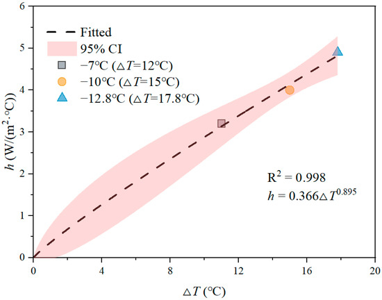
Figure 4.
Fitting results of convective heat transfer coefficients at different temperature differences.
This fitting resulted in an R2 value above 0.99, indicating a high degree of accuracy. Thus, based on the above equation, the temperature changes and freezing processes of the fire pipe at 5 °C were simulated at ambient temperatures of −5 °C, −10 °C, −15 °C, −20 °C, −25 °C, −30 °C, −35 °C, −40 °C, −45 °C, −50 °C, −55 °C, and −60 °C.
2.4. Artificial Neural Network
This study integrates CFD simulations with the ANN to predict freezing thickness in fire pipelines under varying ambient temperatures. Initially, a CFD-based numerical model of the fire pipeline was developed to simulate the freezing process across different temperature conditions. The accuracy of the CFD model was validated through a comparison with experimental data. The CFD simulations generated a freeze thickness dataset comprising over 4115 data points, which was subsequently used to train the ANN model. The input variables for the ANN model included the ambient temperature and time, while the output variable was the freeze thickness. To enhance the model’s generalization capability, the dataset was randomly divided into training, validation, and test sets. By training the ANN model on this dataset, the nonlinear relationships between the ambient temperature, time, and freeze thickness were captured, enabling accurate predictions of the freezing thickness in fire pipelines.
A multilayer feedforward neural network is used as a typical ANN model for modeling [20,29]. The main features of this network are signal forward transmission and error back propagation. In the forward transmission process, the input signal is processed layer by layer from the input layer through the hidden layer to the output layer. The state of neurons in each layer only affects the state of neurons in the subsequent layer. If an output layer fails to receive the expected output, the output layer will turn to back propagation; in addition, the output layer will adjust the network weights according to the prediction error to continuously make the predicted output of the ANN close to the expected output. The topology of the pre-built ANN in this paper is shown in Figure 5 [30]. The mean square error (MSE) of data is utilized to evaluate neural network predictions [31]. The expression for the MSE is as follows:
where ypre and ysim are the predicted and simulated data, respectively, and n is the number of simulated data points. The MSE is a common index to measure the difference between the predicted value and the actual value, and the smaller the value, the smaller the prediction error of the model. The ANN model, constructed using MATLAB R2018a software [32], were trained three times to determine the optimal parameters for each operational scenario and to compare their numerical performance.
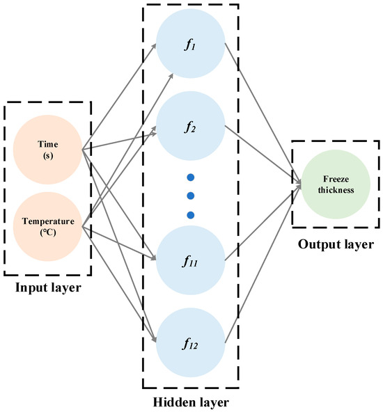
Figure 5.
The schematic topological architecture of the ANN.
3. Results and Discussion
3.1. Freezing Process and Temperature Distribution
3.1.1. Typical Condition
Figure 6 illustrates the freezing conditions over time at an ambient temperature of −35 °C. The results reveal that the onset of freezing is delayed relative to the point at which the temperature reaches 0 °C. This indicates that freezing does not occur immediately after the temperature of the system reaches the freezing point. Instead, a substantial amount of time is spent maintaining thermal equilibrium as the temperature continues to drop, allowing the water within the pipe to cool sufficiently before freezing begins.
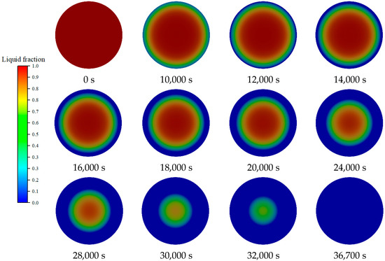
Figure 6.
Freezing process of fire pipe at different times at −35 °C.
Interestingly, noticeable ice formation occurs only during the final stage of the freezing process, where water transitions into ice relatively quickly. The previous stages, which constitute most of the freezing process, are characterized by slower heat transfer. During this period, the system is in a quasi-steady state, with the temperature gradient between the water and surrounding environment gradually decreasing. This prolonged period of thermal stabilization is crucial, as it determines the rate at which the internal water temperature approaches the freezing threshold, thereby delaying the onset of ice formation.
Figure 7 displays the temperature distribution over time at an ambient temperature of −35 °C. Evidently, the temperature within the fire pipe remains above 0 °C for a considerable duration, even after the surrounding temperature drops below the freezing point. This delay in freezing is primarily attributed to the temperature gradient across the pipe wall. These gradients form because the outermost layer of the pipe is influenced by both the ambient conditions and the heat dissipation from the water inside the pipe.
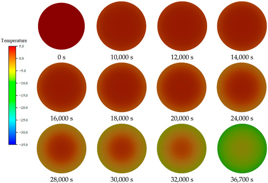
Figure 7.
Temperature distribution inside the fire pipe at different times at −35 °C.
As the system strives to maintain thermal equilibrium, the temperature gradient within the water remains relatively flat for most of the process. The internal water temperature decreases gradually owing to the combined effects of environmental heat loss and the thermal capacity of the water within the pipe [33]. The outermost layer, being in direct contact with the cold ambient environment, experiences a faster temperature drop. However, until the temperature of this layer reaches the freezing point and solidification ensues, heat transfer from the internal water helps maintain a relatively uniform temperature distribution across the pipe’s cross-section. Details regarding the freezing conditions and temperature distributions at other temperatures can be found in the supporting material.
3.1.2. Freeze Thickness
The freeze thickness is defined as the ratio of ice thickness to pipe radius, as illustrated in Figure 8. Freeze thickness measurements were performed over time across a range of environmental temperatures, varying from −5 °C to −60 °C. Figure 9 presents a comprehensive overview of the freezing process at various temperatures, illustrating the times required for the initiation and completion of the freezing process at each temperature. Notably, the temporal variation in freezing thickness at each temperature reveals that the freezing processes at −25 °C and −20 °C deviate from those at other temperatures. Specifically, a noticeable change in the freezing rate (slope) is observed. The results demonstrate that as the ambient temperature drops, the time required for freezing initiation decreases; however, the time required for freezing completion does not follow a strictly linear trend. This observation hints at the existence of a critical temperature where the freezing process becomes nonlinear, possibly owing to complex interactions between heat transfer rates and temperature gradients within the pipe system.
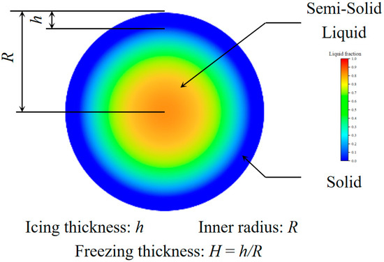
Figure 8.
Schematic of freeze thickness.
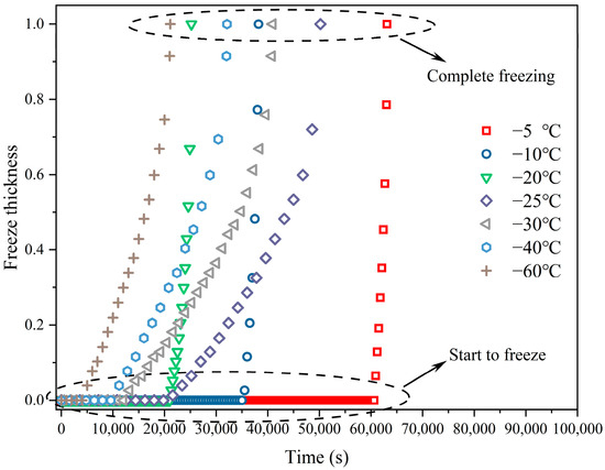
Figure 9.
Freeze thickness with time at different temperatures.
Figure 10 compares the freezing processes at −10 °C, −20, −25, and −40 °C at the same instants. The results reveal that lower ambient temperatures result in higher convective heat transfer coefficients. Under these conditions, freezing begins earlier, and the outer ice layer forms rapidly, while the water within the pipe remains in the liquid phase. Conversely, at higher ambient temperatures, when the outermost pipe layer begins to freeze, the internal liquid fraction approaches the solid phase. Overall, the higher convective heat transfer coefficient at lower ambient temperatures accelerates ice layer formation and limits heat dissipation from the internal water, ultimately prolonging the period required for complete freezing.
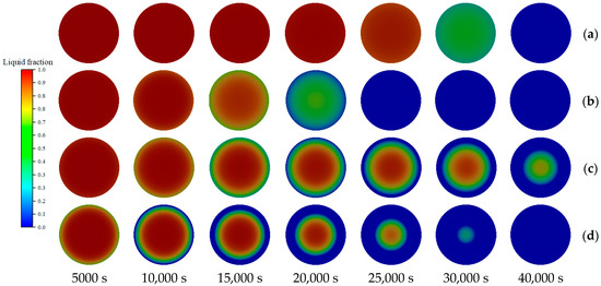
Figure 10.
Comparison of freeze thickness at different times of −10 °C (a), −20 °C (b), −25 °C (c), and −40 °C (d).
3.2. The Establishment and Optimization of the ANN
Freeze thickness was adopted as the final performance metric to evaluate freezing conditions in various working environments. As stated, freeze thickness measurements were conducted over time at environmental temperatures ranging from −5 °C to −60 °C, resulting in a dataset of more than 4115 points, which satisfies the sample size requirements for ML applications. This dataset, with the environmental temperature and time as inputs and freeze thickness as the output, is presented in Table 3. An ANN was trained using the simulated data to predict the freeze thickness of the fire pipe under different temperature conditions by capturing the nonlinear relationships between the inputs and output. The original dataset was randomly split into three subsets: 70% for training, 15% for validation, and 15% for testing [34].
Table 3.
Structure of the dataset.
Notably, the training data only covered temperatures ranging from −5 °C to −50 °C, while data corresponding to temperatures of −55 °C and −60 °C were reserved as external data for verification to prove the generalizability of the selected ANN model.
3.2.1. Determination of the Neuron Number in the Hidden Layer
Analyses revealed that using an excessively limited number of neurons in the hidden layer can result in underfitting, while using too many neurons can lead to problems such as overfitting [35]. Generally, when a neural network contains numerous nodes, the limited information in the training set proves insufficient to train all neurons in the hidden layer, thus leading to overfitting. Even if the training data contain adequate information, the presence of a large number of neurons in the hidden layer increases training time and complicates the realization of optimal results. Hence, selecting an appropriate number of neurons in the hidden layer is crucial for balancing model performance. Most studies rely on the trial-and-error method to determine the number of neurons, primarily owing to the lack of fixed rules for selecting the optimal value. However, an empirical formula can generally be used to estimate the number of neurons (N) as follows:
where s denotes the number of inputs, t represents the number of outputs, and a denotes an arbitrary value, typically ranging from 1 to 10 [34,36]. In this study, the number of inputs for the ANN was set to 2, while the number of outputs was set to 1.
As indicated in Table 4, the final selection of the neuron count was performed by comparing the MSE of the test set when the number of neurons in the hidden layer was varied while maintaining the other parameters at their default values. Notably, the MSE was minimized when the number of neurons was set to 12, yielding a value of 3.04 × 10⁻³.
Table 4.
MSE of the test data with different neuron numbers in the hidden layer.
Although using multiple hidden layers could potentially improve predictive accuracy, the current model, with a single hidden layer, achieved high prediction performance. To avoid unnecessary model complexity, we opted for a simpler architecture, which was sufficient to meet the objectives of this study.
3.2.2. Selection of the Training Function
Notably, a given training function yields two outputs: the trained network and training record. During the training process, this function repeatedly calls the learning algorithm to adjust the weights and thresholds of the network, which terminates the training either when the maximum number of epochs is reached or when the error, as computed by the performance function, falls below a predefined threshold. In an ANN, multiple training functions can be utilized to optimize performance. Given the structure of our dataset, three representative training functions were selected for the ANN: Levenberg-Marquardt backpropagation (trainlm), gradient descent backpropagation (traingd), and gradient descent with adaptive learning rate backpropagation (traingda) [37].
Each training function was tested through three prediction attempts, and the MSE values for each were recorded (Table 5). According to the results, trainlm emerged as the optimal training function, with an MSE of 5.00 × 10⁻³.
Table 5.
MSE of the test data with different training functions.
3.2.3. Selection of the Activation Function
The activation function, also known as the transfer function, is a critical component of an ANN and must be continuously differentiable. Common activation functions include S-shaped logarithmic functions (logsig), tangent (tansig) functions, and linear functions (purelin) [38]. To maximize computational efficiency, both the activation function and its derivative should be as simple as possible. In this study, the nonlinear transfer functions logsig and tansig were selected to form the input layer to hidden layer connection, while the purelin function was chosen to form the hidden layer to output layer connection. The optimal combination of activation functions for the ANN model was determined by comparing the MSE. As indicated in Table 6, the tansig and purelin function combination yielded the smallest MSE of 2.00 × 10⁻³.
Table 6.
MSE of test data with different activation functions.
3.3. Performance of the Selected ANN
As outlined in Section 3.2, the optimal configuration of the ANN model contained 12 neurons in the hidden layer, utilized trainlm as its training function and employed tansig-purelin as its activation function. After training the optimized ANN model, its performance was evaluated on the validation set and test set, as illustrated in Figure 11. The optimal performance of the model was observed at epoch 212, when its MSE on the test set reached 6.62 × 10⁻⁴.
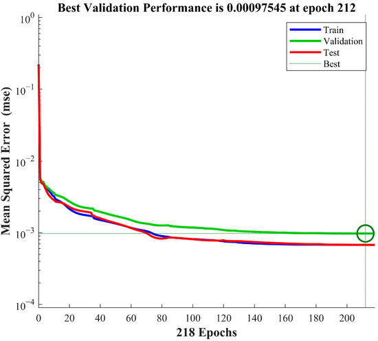
Figure 11.
Performance of the selected topology.
Figure 12 displays the regression performance of the model. Regression coefficient (R) is an important statistical index to measure the degree of model fitting. An R value close to 1 indicates that the model can fit the data well, and the correlation between the predicted results and the real data is strong. As depicted, the R of the model exceeds 0.98 for the validation and test sets, indicating excellent performance. A high R value on the training set confirms the model’s ability to fit the data well. The remarkable performance of the model on the test set demonstrates its good generalization ability, which enables it to predict the freeze thickness of the fire pipe under conditions different from those included in the training dataset.
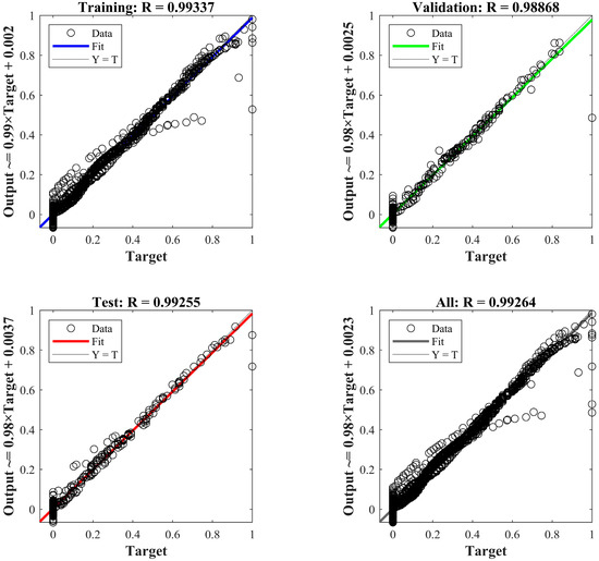
Figure 12.
Regression of training, validation, and test data for the selected topology (neuron number: 12, training function: trainlm, activation function: tansig–purelin).
3.4. Prediction of Freeze Thickness with the ANN
The generalization ability of a model is reflected by its performance on previously unseen input data, such as those included in test sets or external data [39]. Figure 13 illustrates the freezing thickness predicted over time by the ANN model at two temperatures of −55 °C and −60 °C. As depicted, the red curve (prediction) and red squares (simulation) demonstrate good agreement at −55 °C, indicating that the ANN model accurately captures the increasing trend of freezing thickness over time. The model not only predicts the increase rate of freezing thickness but also achieves high accuracy in this prediction at different stages of the freezing process, including the onset and stabilization phases. Meanwhile, at −60 °C, the blue curve (prediction) and blue triangle (simulation) demonstrate the ANN model’s ability to predict freezing thickness under harsher conditions. Although the prediction curve slightly deviates from the simulation result, the overall alignment between the two is remarkable. This generalization is particularly notable during the early- and mid-icing stages (as highlighted in the enlarged portion at the bottom left of the figure), where the predictions closely match the simulation results for both −55 °C and −60 °C.
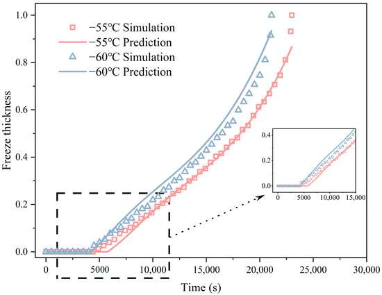
Figure 13.
Comparison of predicted results with simulated data different from the training data.
The generalization ability of the ANN model is further demonstrated by its consistent performance across the temperatures it was trained on (−5 °C to −50 °C) and unseen (−55 °C and −60 °C) temperatures. This highlights the ANN model’s capacity to extend its learned patterns to new scenarios, accurately predicting freezing thickness without being overly dependent on the specific conditions of the training data.
4. Conclusions
A model for predicting the freeze thicknesses of fire pipes under low-temperature conditions was successfully developed by integrating CFD with an ANN. Experimental data were validated using a trial-and-error method, and a fitting formula () for the convective heat transfer coefficient and temperature difference was derived based on the simulation results. The validated CFD model generated a comprehensive dataset for training the ANN, thus enabling highly accurate predictions of freeze thickness. Furthermore, the CFD results revealed a nonlinear relationship among the freeze thickness of the fire pipe, ambient temperature, and time. The optimal ANN architecture—comprising 12 neurons, the trainlm training function, and the tansig–purelin activation function—demonstrated excellent predictive performance, with an MSE of 6.62 × 10⁻⁴ and a regression coefficient (R) greater than 0.98 on all datasets. Furthermore, the predictions of the ANN model closely matched the simulated data not only across the training temperature range (−5 °C to −50 °C) but also across unseen temperatures (−55 °C and −60 °C), highlighting its excellent generalizability. Future research could explore the effects of different pipe thicknesses and geometries on freezing thickness predictions to enhance the model’s practical relevance.
Author Contributions
Conceptualization, Y.H. and J.Z.; methodology, Y.Z.; software, Y.Z.; validation, Y.G., Y.Z. and Y.D.; formal analysis, Y.H.; investigation, Y.H.; resources, Y.H.; writing—original draft preparation, Y.H.; writing—review and editing, Y.Z.; visualization, Y.G.; supervision, J.Z.; project administration, Y.D.; funding acquisition, J.Z. All authors have read and agreed to the published version of the manuscript.
Funding
The authors would like to acknowledge financial support sponsored by the Science and Technology Project of State Grid Corporation of China (No. 5700-202320280A-1-1-ZN).
Institutional Review Board Statement
Not applicable.
Informed Consent Statement
Not applicable.
Data Availability Statement
The original contributions presented in the study are included in the article, further inquiries can be directed to the corresponding author.
Conflicts of Interest
The authors declare no conflicts of interest.
Abbreviations
The following abbreviations are used in this manuscript:
| CFD | Computational Fluid Dynamics |
| ANN | Artificial Neural Network |
| MSE | Mean Square Error |
| ML | Machine Learning |
References
- Guo, T.-N.; Fu, Z.-M. The fire situation and progress in fire safety science and technology in China. Fire Saf. J. 2007, 42, 171–182. [Google Scholar] [CrossRef]
- Peng, T.; Ke, W. Urban fire emergency management based on big data intelligent processing system and Internet of Things. Optik 2023, 273, 170433. [Google Scholar] [CrossRef]
- Duan, L.; Hou, X. Review of automatic fire water monitor system. J. Phys. Conf. Ser. 2021, 1894, 012013. [Google Scholar] [CrossRef]
- Khan, F.; Ahmed, S.; Yang, M.; Hashemi, S.J.; Caines, S.; Rathnayaka, S.; Oldford, D. Safety challenges in harsh environments: Lessons learned. Process Saf. Prog. 2015, 34, 191–195. [Google Scholar] [CrossRef]
- Park, Y.-S.; Seong, H.-S.; Suh, J.-S. Numerical Analysis of Freezing Phenomena of Water around the Channel Tube of MF Evaporator. J. Korean Soc. Manuf. Process Eng. 2020, 19, 114–120. [Google Scholar] [CrossRef]
- Vishnoi, K. Piping layout for fire sprinkler system: An overview. Int. J. Eng. Appl. Sci. 2017, 4, 257513. [Google Scholar] [CrossRef]
- Park, Y.-S.; Suh, J.-S. Numerical Analysis of Freezing Phenomena of Water in a U-Type Tube. Korean Soc. Manuf. Process Eng. 2019, 18, 52–58. [Google Scholar] [CrossRef]
- Kim, B.-H.; Kwak, J.-J.; Seo, S.-M.; Kim, Y.-B.; Nam, J.-S.; Lim, S.-S. Freezing-Prediction System of Outdoor Horizontal Fire Pipe Using Metal Heater. Fire Sci. Eng. 2023, 37, 44–51. [Google Scholar] [CrossRef]
- Lee, C.; Suh, J.-S. Numerical Analysis on the Freezing Process of Internal Water Flow in a L-Shape Pipe. Korean Soc. Manuf. Process Eng. 2018, 17, 144–150. [Google Scholar] [CrossRef]
- Wang, W.; Kong, Y.; Wang, F.; Yang, L.; Niu, Y. Anti-freezing prediction model for different flow patterns of air-cooled heat exchanger. Int. J. Heat Mass Transf. 2020, 153, 119656. [Google Scholar] [CrossRef]
- Yang, M.; Yang, S.; Kim, W. Anti-freeze Application in Fire Extinguishing Facility Piping for a Warehouse Building. J. Korean Soc. Hazard Mitig. 2020, 20, 233–237. [Google Scholar] [CrossRef]
- Jeong, G.; Ahn, B.; Seong, Y.; Kim, K. Numerical Analysis of Phase Change and Natural Convection Phenomena During Pipe Freezing Process. In Proceedings of the ASME Pressure Vessels and Piping Conference, Vancouver, BC, Canada, 5–9 August 2002. [Google Scholar] [CrossRef]
- Mishra, K.B.; Wehrstedt, K.-D. Underground gas pipeline explosion and fire: CFD based assessment of foreseeability. J. Nat. Gas Sci. Eng. 2015, 24, 526–542. [Google Scholar] [CrossRef]
- Park, Y.-S.; Seong, H.-S.; Suh, J.-S. An Analytical Study on the Heat Transfer Characteristics of MF Evaporation Tubes Attached with a Fin. J. Korean Soc. Manuf. Process Eng. 2021, 20, 48–56. [Google Scholar] [CrossRef]
- Bakas, I.; Kontoleon, K.J. Meta-Narrative Review of Artificial Intelligence Applications in Fire Engineering with Special Focus on Heat Transfer through Building Elements. Fire 2023, 6, 261. [Google Scholar] [CrossRef]
- Cho, H.; Seo, S.; Heo, C.; Kwak, J.; Kim, Y.; Park, J.; Lee, S.; Lim, S. Performance estimation of freeze protection system for outdoor fire piping by using AI algorithm. J. Mech. Sci. Technol. 2023, 37, 5093–5101. [Google Scholar] [CrossRef]
- Kim, H.; Lee, J.; Kim, T.; Park, S.J.; Kim, H.; Jung, I.D. Advanced thermal fluid leakage detection system with machine learning algorithm for pipe-in-pipe structure. Case Stud. Therm. Eng. 2023, 42, 102747. [Google Scholar] [CrossRef]
- Zhong, Y.; Liu, F.; Huang, G.; Zhang, J.; Li, C.; Ding, Y. Thermogravimetric experiments based prediction of biomass pyrolysis behavior: A comparison of typical machine learning regression models in Scikit-learn. Mar. Pollut. Bull. 2024, 202, 116361. [Google Scholar] [CrossRef]
- Abiodun, O.I.; Jantan, A.; Omolara, A.E.; Dada, K.V.; Mohamed, N.A.; Arshad, H. State-of-the-art in artificial neural network applications: A survey. Heliyon 2018, 4, e00938. [Google Scholar] [CrossRef] [PubMed]
- Hecht-Nielsen, R. III.3.—Theory of the Backpropagation Neural Network; Academic Press: Cambridge, MA, USA, 1992. [Google Scholar] [CrossRef]
- Salakhi, M.; Eghtesad, A.; Afshin, H. Heat and mass transfer analysis and optimization of freeze desalination utilizing cold energy of LNG leaving a power generation cycle. Desalination 2022, 527, 115595. [Google Scholar] [CrossRef]
- Najafi Khaboshan, H.; Jaliliantabar, F.; Abdullah, A.A.; Panchal, S.; Azarinia, A. Parametric investigation of battery thermal management system with phase change material, metal foam, and fins; utilizing CFD and ANN models. Appl. Therm. Eng. 2024, 247, 123080. [Google Scholar] [CrossRef]
- Luo, W. Study on Thermal Environment of Underground Tunnel Entrance Section and Electric Tracing Heat Preservation of Fire Pipe in Cold Region; Xi ’an University of Architecture and Technology: Xi’an, China, 2023. (In Chinese) [Google Scholar]
- Matsson, J.E. An Introduction to Ansys Fluent 2023; SDC Publications: Mission, KS, USA, 2023. [Google Scholar]
- Bonales, L.J.; Rodriguez, A.C.; Sanz, P.D. Thermal conductivity of ice prepared under different conditions. Int. J. Food Prop. 2017, 20, 610–619. [Google Scholar] [CrossRef]
- Voller, V.R.; Prakash, C. A fixed grid numerical modelling methodology for convection-diffusion mushy region phase-change problems. Int. J. Heat Mass Transf. 1987, 30, 1709–1719. [Google Scholar] [CrossRef]
- Lewis, J.S. Heat transfer predictions from mass transfer measurements around a single cylinder in cross flow. Int. J. Heat Mass Transf. 1971, 14, 325–329. [Google Scholar] [CrossRef]
- Shibani, A.A.; Özisik, M.N. Freezing of liquids in turbulent flow inside tubes. Can. J. Chem. Eng. 1977, 55, 672–677. [Google Scholar] [CrossRef]
- Zhong, W.; Wang, S.; Wu, T.; Gao, X.; Liang, T. Optimized Machine Learning Model for Fire Consequence Prediction. Fire 2024, 7, 114. [Google Scholar] [CrossRef]
- Agatonovic-Kustrin, S.; Beresford, R. Basic concepts of artificial neural network (ANN) modeling and its application in pharmaceutical research. J. Pharm. Biomed. Anal. 2000, 22, 717–727. [Google Scholar] [CrossRef]
- Velmurugan, C.; Subramanian, R.; Thirugnanam, S.; Anandavel, B. Experimental study and prediction using ANN on mass loss of hybrid composites. Ind. Lubr. Tribol. 2012, 64, 138–146. [Google Scholar]
- Installation Guide. In MATLAB® & Simulink®; R2018a; Mathworks: Natick, MA, USA, 1996.
- Zhou, G.; He, J. Thermal performance of a radiant floor heating system with different heat storage materials and heating pipes. Appl. Energy 2015, 138, 648–660. [Google Scholar] [CrossRef]
- Zhong, Y.; Ding, Y.; Jiang, G.; Lu, K.; Li, C. Comparison of Artificial Neural Networks and kinetic inverse modeling to predict biomass pyrolysis behavior. J. Anal. Appl. Pyrolysis 2023, 169, 105802. [Google Scholar] [CrossRef]
- Çepelioğullar, Ö.; Mutlu, İ.; Yaman, S.; Haykiri-Acma, H. A study to predict pyrolytic behaviors of refuse-derived fuel (RDF): Artificial neural network application. J. Anal. Appl. Pyrolysis 2016, 122, 84–94. [Google Scholar] [CrossRef]
- Karsoliya, S.; Azad, M.A.K. Approximating Number of Hidden layer neurons in Multiple Hidden Layer BPNN Architecture. Int. J. Eng. Trends Technol. 2012, 3, 714–717. [Google Scholar]
- Çepelioğullar, Ö.; Mutlu, İ.; Yaman, S.; Haykiri-Acma, H. Activation energy prediction of biomass wastes based on different neural network topologies. Fuel 2018, 220, 535–545. [Google Scholar] [CrossRef]
- Taheri, S.; Brodie, G.; Gupta, D. Optimised ANN and SVR models for online prediction of moisture content and temperature of lentil seeds in a microwave fluidised bed dryer. Comput. Electron. Agric. 2021, 182, 106003. [Google Scholar] [CrossRef]
- Rabin, M.R.I.; Hussain, A.; Alipour, M.A.; Hellendoorn, V.J. Memorization and generalization in neural code intelligence models. Inf. Softw. Technol. 2023, 153, 107066. [Google Scholar] [CrossRef]
Disclaimer/Publisher’s Note: The statements, opinions and data contained in all publications are solely those of the individual author(s) and contributor(s) and not of MDPI and/or the editor(s). MDPI and/or the editor(s) disclaim responsibility for any injury to people or property resulting from any ideas, methods, instructions or products referred to in the content. |
© 2025 by the authors. Licensee MDPI, Basel, Switzerland. This article is an open access article distributed under the terms and conditions of the Creative Commons Attribution (CC BY) license (https://creativecommons.org/licenses/by/4.0/).