A PINN-LSTM Model for Real-Time Gas Concentration Prediction in Mine Conveyor Belt Fires

Abstract

Accurate prediction of toxic gas concentrations during conveyor-belt fires is essential for ensuring mine safety, yet the nonlinear, time-varying, and turbulent characteristics of underground environments pose significant challenges for real-time forecasting. This study proposes a Physics-Informed Neural Network–Long Short-Term Memory (PINN-LSTM) hybrid model that integrates the one-dimensional convection–diffusion equation as a physical constraint with the sequential learning capability of an LSTM. Full-scale mine tunnel combustion experiments and Fire Dynamics Simulator (FDS) numerical simulations under multiple wind speeds and distances were conducted for model training and validation. The results indicate that the proposed PINN-LSTM achieves the lowest error metrics under all test conditions. The model reduced MSE and RMSE by 70–78% and 65–73%, respectively, compared with traditional LSTM models, and by 8–12% compared with the PINN-TCN variant. The proposed PINN-LSTM achieves the lowest error under all conditions. The PINN-LSTM model has strong prediction accuracy, physical interpretability, and real-time reasoning ability, providing a reliable and physically consistent solution for intelligent gas monitoring and early warning systems in underground fire scenarios.

1. Introduction

As the coal industry has developed and production scales have continuously expanded, underground coal mine transportation has evolved from manual methods to mechanized systems [1,2]. Belt conveyors have largely replaced traditional vehicle- and car-based transportation due to their high efficiency, advanced automation, robust conveying capacity, reliable performance, and ease of maintenance [3,4]. Consequently, they are now widely adopted in coal mine production and transportation. The unique environment of underground coal mines, characterized by relatively low oxygen concentrations and complex ventilation conditions, poses significant fire risks. Once initiated, fires can spread rapidly and are difficult to control, often leading to severe economic losses and casualties [5,6]. Crucially, fires generate substantial quantities of toxic and harmful gases, such as CO and HCl. Fluctuations in the concentrations of these gases are directly indicative of the severity of the disaster [7]. Traditional gas concentration prediction methods, relying primarily on manual inspections and fixed sensor monitoring, suffer from limitations including restricted monitoring range, slow response times, and insufficient accuracy [8,9]. Therefore, developing an efficient and accurate gas concentration prediction method is crucial for enhancing coal mine safety management.

Real-time gas concentration prediction during coal mine belt fires faces significant challenges stemming from the time-varying, nonlinear, and noise-corrupted nature of the data [10,11]. Gas concentrations exhibit clear temporal dependencies, necessitating the consideration of historical data for accurate future predictions [12]. The gas diffusion process is influenced by a multitude of factors, including environmental parameters such as wind speed, direction, and temperature, as well as fire characteristics like intensity and burning rate [8,13,14,15,16,17]. These interacting influences result in the nonlinear behavior of gas concentration changes. Furthermore, sensor measurements are inherently susceptible to noise interference, making the extraction of valid information a critical concern [18,19]. Traditional gas concentration prediction methods often struggle to effectively address these challenges, leading to limitations in their predictive accuracy and reliability.

Deep learning algorithms, particularly Recurrent Neural Networks (RNNs) and their variants such as Long Short-Term Memory (LSTM) networks and Gated Recurrent Units (GRUs), excel at processing time series data and are thus widely applied in gas concentration prediction.

Beyond LSTMs and GRUs, other deep learning architectures have also been employed for this task. For instance, Convolutional Neural Networks (CNNs), known for their proficiency in handling spatial data, can extract spatial features from gas concentration datasets [20,21,22,23]. Notably, One-Dimensional Convolutional Neural Networks (1D-CNNs) are particularly well-suited for time series data, capable of capturing local temporal features [24,25]. Furthermore, Generative Adversarial Networks (GANs) have been applied to gas concentration prediction. For example, one study proposed an improved TCN-TimeGAN-based intelligent prediction method for coal mine gas concentration [26,27,28,29]. This method leverages the characteristics of GANs to mitigate the overfitting issue associated with small gas data samples. It utilizes a Temporal Convolutional Network (TCN) to expand the receptive field for extracting long-term temporal features [26,27,30]. However, deep learning algorithms typically demand extensive training data, involve complex training procedures, and their prediction results often lack interpretability [31,32].

Traditional physics-based models offer interpretability but are often computationally intensive and insufficiently adaptable for real-time forecasting. Purely data-driven models (e.g., LSTM, GRU) can learn temporal regularities yet typically ignore the governing equations of gas diffusion, limiting extrapolation and physical plausibility [33,34,35]. The Physics-Informed Neural Network–Long Short-Term Memory (PINN-LSTM) integrates physics-based constraints with deep sequence modeling to close this gap, enforcing adherence to diffusion laws while improving predictive accuracy [36,37,38]. In this hybrid architecture, the PINN encodes spatial relationships and physical residuals (e.g., PDE and boundary/initial conditions), whereas the LSTM captures long-range temporal dependencies; together they balance spatial and temporal learning, enabling stable and real-time capable predictions.

This study represents the first application of this hybrid framework to gas concentration prediction under varying wind speeds and fire source intensities. We conducted full-scale gallery experiments on belt combustion and performed numerical simulations of belt combustion under different wind speeds. Comparisons between the predicted results and the experimental and numerical simulation outcomes validate the superior adaptability and stability of the proposed model over existing methods, offering a novel and effective solution for belt fire prediction.

2. Materials and Methods

This study proposes a PINN-LSTM hybrid model designed to predict gas concentration values within a roadway under varying wind speeds. This is achieved by utilizing independent parameters, including wind speed, roadway length, and effective diffusion coefficient. The PINN-LSTM hybrid model employs data-driven techniques while integrating fundamental physical equations to achieve higher accuracy than traditional, standalone time series prediction methods.

2.1. The Physics-Informed LSTM Model

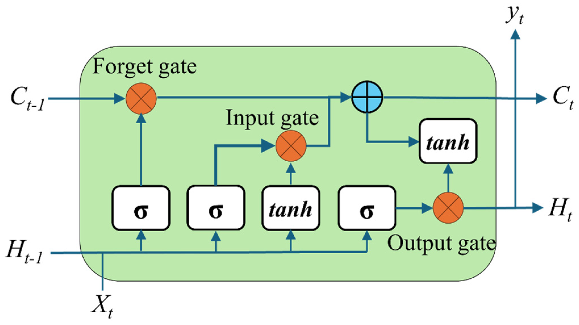
The PINN-LSTM model incorporates memory cells capable of storing information over arbitrary time intervals, along with three regulating gates, as depicted in Figure 1.

These three gates-the forget gate f_t, input gate i_t, and output gate o_t-are responsible for controlling data flow and determining how the memory cell updates at each timestep. Because the gates control information flow, each uses a Sigmoid activation to map its pre-activation to [0, 1]. The input gate regulates how much of the candidate cell content is written to the memory; the forget gate determines how much of the previous cell state is retained; the output gate controls how much of the updated cell state is exposed in the hidden state. Concretely, at the forget gate, the current input and the previous hidden state are concatenated and passed through a sigmoid,

$$f_t=\sigma (W_{fx}{x}_t+W_{fh}{h}_{t-1}+b_f)$$

(1)

$$i_t=\sigma (W_{ix}{x}_t+W_{ih}{h}_{t-1}+b_i)$$

(2)

$$o_t=\sigma (W_{ox}{x}_t+W_{oh}{h}_{t-1}+b_o)$$

(3)

$${\tilde{c}}_t=\tanh (W_h{x}_t+W_h{h}_{t-1}+b_h)$$

(4)

where σ is the sigmoid activation function, tanh is the hyperbolic tangent activation function, ʘ denotes element-wise multiplication, x_t is the input features at time t, h_t−1 is the output of the previous time step, ${\stackrel{-}{\mathit{C}}}_{\mathit{t}}$ is the candidate memory cell at time t, W_fx, W_ix, W_ox, W_h is the weights that govern the behavior of the c_t, f_t, i_t, and o_t gates, b_f, b_i, b_o, b_h is the biases that govern the behavior of the c_t, f_t, i_t, and o_t gates.

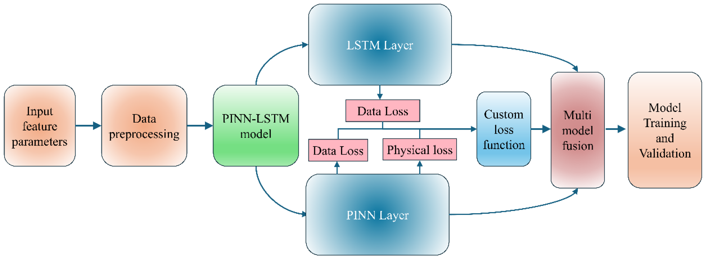
The PINN-LSTM model adopts a dual-branch architecture that couples PINN with a LSTM module. The PINN branch enforces gas-diffusion physics via residual losses from the governing PDE and boundary/initial conditions, encoding spatial dependencies and physical plausibility. The LSTM branch models long-range temporal dependencies in the measured sequences. Joint training fuses the two signals, yielding predictions that remain consistent with diffusion dynamics while capturing complex temporal patterns.

The PINN branch comprises two fully connected hidden layers (64 and 32 units) with ReLU activations; batch normalization is applied to stabilize gradients and accelerate convergence. A final fully connected head outputs gas-concentration estimates. Physical consistency is enforced via a composite loss that minimizes the residual of the convection–diffusion equation and adds boundary/initial-condition penalties, guiding the network toward PDE-consistent solutions.

The LSTM branch models sequential structure in gas-concentration time series. It uses a single LSTM layer with 64 units to capture long-range dependencies via its hidden and cell states. The layer’s output is then passed through a ReLU-activated projection to increase representational capacity, followed by a fully connected head that generates the predicted gas-concentration values.

Multi-model fusion is performed at two complementary levels. (1) Optimization level: a composite loss jointly minimizes the PINN’s physics-based residuals (e.g., PDE and boundary/initial constraints) and the supervised, data-driven errors from both the PINN and LSTM branches; learnable weights balance the physics and data terms to optimize overall predictive performance. (2) Representation/output level: the two branches, trained jointly but parameter-wise independent, produce complementary predictions/embeddings that are merged in a fusion layer via learnable weighting to yield the final gas-concentration estimate. This two-stage fusion leverages the strengths of physics-guided modeling (consistency and extrapolability) and deep sequence learning (long-range temporal modeling), thereby improving generalization across depths and prediction horizons and enhancing accuracy. The integrated design (Figure 1) yields a unified architecture that balances theoretical constraints with data-driven learning for robust gas-concentration forecasting.

The model ingests aligned inputs with identical feature sets and time windows, which are routed in parallel to the PINN and LSTM branches. In the PINN path, fully connected layers project inputs into latent states used both to compute PDE residuals that enforce physical consistency and to produce a preliminary concentration estimate. In the LSTM path, recurrent layers encode long-range temporal dependencies and generate a parallel estimate/embedding. The two branch outputs are concatenated along the last dimension and fed into a learnable fusion head to yield a single gas-concentration prediction. Joint training with a composite loss balances physics-based penalties and supervised errors, so the final outputs remain consistent with diffusion physics while leveraging data-driven temporal patterns (Figure 2).

The PINN-LSTM hybrid model effectively combines physical laws with data-driven learning, leveraging both theoretical principles and empirical data. The inclusion of a PINN ensures the integration of domain-specific physical constraints, thereby guaranteeing that predictions maintain physical consistency and realism. Simultaneously, the LSTM component, with its proven ability to model sequential dependencies and capture long-term temporal patterns, is particularly effective for multi-temporal wave speed prediction.

By jointly leveraging physics-guided spatial modeling and deep sequence learning, the fused PINN–LSTM attains a principled balance between spatial structure and temporal dynamics. The PINN component enforces diffusion laws and boundary/initial conditions, while the LSTM component captures long-range dependencies and regime shifts that stand-alone physics-based or purely data-driven models often miss. Consequently, the hybrid framework delivers higher accuracy, better stability, and stronger generalization across prediction horizons and depths, and is well suited to noisy, nonstationary, and sensor-limited underground environments.

2.2. The Loss Function Based on Physical Information

To predict the time-dependent concentrations of CO and HCl gases generated during a conveyor belt fire in a roadway, the core physical principle is governed by the convection–diffusion equation, which describes gas transport and dispersion. For the gas concentration C_(x,t) in a conveyor roadway fire, its one-dimensional form can be expressed as:

$${\displaystyle \frac{\partial C(x,t)}{\partial t}}+u(x,t){\displaystyle \frac{\partial C(x,t)}{\partial x}}=D_{eff}{\displaystyle \frac{{\partial }^{2}C(x,t)}{\partial x^2}}+S(x,t)$$

(5)

where C(x,t) is the concentration of gas in the tunnel at a distance of x m from the fire source and at time t s (%), ∂C/∂t is the rate of change in gas concentration over time (% s⁻¹), u(x,t) is the average wind speed along the axis of the tunnel (m s⁻¹), D_eff is effective diffusivity, S(x,t) is the source term, representing the rate of gas generation from the fire.

In the proposed PINN-LSTM framework, the average wind speed u(x,t) is treated as a measured quantity, obtained from wind sensors placed upstream of the fire source during both the experimental and simulation phases. It is not a learned parameter within the PINN model.

The effective diffusion coefficient D_eff is modeled as a constant during each training run. It is treated as a tunable hyperparameter during training to reflect environmental variability.

The gas generation term S(x,t) is directly related to the heat release rate (HRR) and mass loss rate (MLR) of the combustion reaction. According to the experimental results of the cone calorimeter [39], the average HRR of the PVC conveyor belt under 15–60 kW/m² thermal radiation is 50–110 kW/m ², corresponding to an MLR of approximately 0.032–0.045 g·s⁻¹·cm⁻². By normalizing the CO and HCl yields, a reasonable order of magnitude for S(x,t) can be obtained as approximately 10⁻⁵–10⁻³ mol·m⁻³·s⁻¹.

Therefore, this article considers the gas generation rate S(x,t) as a physical hyperparameter that can be adjusted within the above range, rather than a purely empirical parameter, to reflect the intensity differences during the combustion stage.

The spatial domain and temporal domain are:

$$\begin{array}{cc}x\in [0,L],& t\in [0,T]\end{array}$$

(6)

where L is the length of the tunnel (m), T is the duration of monitoring data (s).

At t = 0, the initial gas concentration is assumed to be ambient:

$$C_{(x,0)}=0$$

(7)

The boundary conditions for the intake and return can be expressed as:

$$C(0,t)=0$$

(8)

$${\displaystyle \frac{\partial C_{(L,t)}}{\partial x}}=0$$

(9)

The source term models gas generation as a spatial delta function:

$$S(x,t)=S(t)\delta (x-x_s)$$

(10)

where S(t) is a time-dependent source strength, δ(x − xs) is the Dirac delta function used to represent a point source, x_s is the fire source location.

In the PINN-LSTM hybrid model, the core idea is to incorporate the residual of the aforementioned physical equation as a component of the loss function. The LSTM model predicts the gas concentration, C_pred(xi,ti), at specific sensor locations over a future time period. Leveraging the automatic differentiation capabilities of deep learning frameworks, we compute the partial derivatives of the LSTM model’s predicted output, C_pred(xi,ti), with respect to time (t) and space (x). This yields ∂C_pred/∂t, ∂C_pred/∂x and ∂²C_pred/∂x². These calculated partial derivatives, along with the wind speed u_(x,t), the effective diffusion coefficient D_eff, and other physical parameters optimized as physics-informed enhancement hyperparameters, are then substituted into the convection–diffusion equation. The residual, R(x,t), is obtained by subtracting the right-hand side of the equation from the left-hand side, as expressed in Equation (11):

$$R(x,t)={\displaystyle \frac{\partial C_{pred}}{\partial t}}+u(x,t){\displaystyle \frac{\partial C_{pred}}{\partial x}}-D_{eff}{\displaystyle \frac{{\partial }^2{C}_{pred}}{\partial x^2}}-S(x,t)$$

(11)

Since u(x,t) and S(x,t) are obtained through experiments, this expression is fully computable using automatic differentiation on the predicted concentration field C_pred(x_i,t_i).

The data loss quantifies the discrepancy between the model’s predicted values and the actual monitored values. This is computed using the mean squared error (MSE) for both the PINN model L_P and the LSTM model L_d. By comparing the predicted outputs of the PINN and LSTM models against their respective actual values, the individual data losses for each model are determined.

The physics loss is then calculated by sampling residuals at N_c collocation points (x_i,t_i), distributed uniformly over the spatiotemporal domain:

$$L_p={\displaystyle \frac{1}{N}}{\displaystyle \sum _{k=1}^N(R(x_k,t_k)}{)}^2$$

(12)

where N is the number of spatiotemporal points used to calculate physical losses.

In practice, these collocation points include uniformly distributed interior points within the domain, and additional samples near the fire source to capture steep gradients.

The data loss accounts for all measured gas concentration values at sensor locations (x_s,t_j):

$$L_d={\displaystyle \frac{1}{N_s{N}_t}}{\displaystyle \sum _{s=1}^{N_s}{\omega }_s}{\displaystyle \sum _{j=1}^{N_t}{(C_{pred}(x_s,t_j)-C_{obs}(x_s,t_j))}^2}$$

(13)

where N_s is the number of sensors, N_t is the number of time steps, ω_s is the weight assigned to each sensor, C_pred(x_s,t_j) is the predicted value, C_obs(x_s,t_j) is the observed value.

Boundary and initial conditions are incorporated as soft constraints using additional penalty losses:

$$L_{BC}={\displaystyle \frac{1}{N_{BC}}}\left({\displaystyle \sum _{j=1}^{N_t}{(C_{pred}(0,t_j)-C_{in})}^2+{\displaystyle \sum _{j=1}^{N_t}{(\frac{\partial C_{pred}(L,t_j)}{\partial x})}^2+{\displaystyle \sum _{j=1}^{N_t}{(C_{pred}(x_i,0)-C_0(x_i))}^2}}}\right)$$

(14)

where C_in = 0 at the intake, $\partial C_{pred}(L,t_j)$ at the return airway, C₀(x) = 0 is the initial concentration profile, N_BC is the total number of boundary and initial condition samples.

The final loss function is then defined as a weighted sum of the data loss L_{LSTM_data}, the physical loss L_{PINN_data} and the boundary and initial conditions penalty losses L_BC:

$$L_{PINN-LSTM}=\lambda L_d+(1-\lambda )L_P+\alpha L_{BC}$$

(15)

where λ is a constant between 0–1, α is the penalty loss coefficient, usually taken as 0.01.

The total loss function integrates physical guided loss and combined data loss to guide the training process of the PINN-LSTM model. In addition, this expression of total loss ensures that model optimization is influenced by both physical information and model prediction performance, thereby improving the accuracy of gas concentration prediction.

The calculated loss is then back-propagated through the neural network to compute the gradients required for updating the LSTM unit’s weights and biases. Subsequently, a stochastic optimization method is employed to minimize the error generated by the loss function.

$$(\widehat{\theta })=\arg {\min }_{(\theta )}L(\theta )$$

(16)

Given the non-linear nature of the network’s loss function, the ADAM gradient-based minimization algorithm is utilized. Training can be stopped once the optimization algorithm completes the preset number of iterations.

2.3. Training Parameter Selection and Validation

To ensure the convergence and generalization stability of the PINN-LSTM model, system validation was conducted on the main training parameters before formal model training.

Under the condition of fixed other parameters (batch size = 64, learning rate = 1 × 10⁻³), set the training epochs to 20, 30, 40, 50, 80 and 100 for testing. Record the training and validation loss curves for each setting, observe the convergence trend of the validation set loss with epochs, and calculate the error change rate. When the validation loss decreases by less than 0.001 within 5 consecutive epochs, it is considered to have converged.

As shown in Figure 3, the training and validation losses tend to stabilize after 25–40 epochs and no longer decrease after 50 epochs. Continue training until 80 or 100 epochs to improve by less than 1%. Therefore, the upper limit of a single training session is set to 50 epochs.

Monitor the Validation Loss during the training process. If the validation loss does not improve within 10 consecutive epochs (i.e., the decrease is less than 0.001), the training will be terminated early. This strategy controls the actual training epochs between 25–45 in most scenarios, effectively avoiding overfitting of the model in small sample situations.

To prevent overfitting of the model during later training, the validation set loss is continuously monitored during the training process. After each epoch, record the verification error and compare it with the current minimum value:

$$L_{best}=\min \left(L_{val}^{(1)},L_{val}^{(1)}\cdots ,L_{val}^{(N)}\right)$$

(17)

When the new validation error is lower than L_best, the model immediately saves the weights for that round. After the training is completed, the testing phase uses the weight with the lowest validation error (best epoch checkpoint) for prediction.

This optimal model selection method based on the validation set is equivalent to an “indirect early stopping” mechanism-even if the total training epochs are fixed at 50, it can avoid overfitting caused by too many iterations. The validation error curve indicates that most training reaches its minimum value between epochs 25–40, followed by slight oscillations, so the final model usually corresponds to the weights of the interval.

2.4. Model Parameters and Hyperparameters Tuning

Machine learning performance is governed by two categories of quantities: model parameters and hyperparameters. Model parameters—weights and biases—are learned during training by optimizing a loss function. Through iterative updates, they encode how input features map to outputs to minimize the discrepancy between predictions and observations.

Hyperparameters, by contrast, are specified before training and typically remain fixed during a single training run. They control the learning dynamics and model capacity, such as learning rate, batch size, number of training epochs, network depth and hidden width, as well as regularization settings and optimizer choices. Appropriate hyperparameter settings improve convergence speed, stability, and generalization, whereas poor choices can lead to underfitting, overfitting, or slow/unstable training.

In this study, we optimized hyperparameters related to the LSTM unit architecture: the learning rate, batch size, hidden dimension of the neural network layer, and λ. Additionally, hyperparameters based on the physics-informed equation, specifically the gas generation rate and the effective diffusion coefficient, were also optimized. Detailed parameter information is provided in

Table 1. The LSTM cell architecture and physics-based hyperparameter sets and their ranges are used for optimization.

Type	Hyperparameter	Range
LSTM	Batch	32~128
	Hidden dimension	8~128
	Learning rate	1 × 10−4~1
	λ	0.2~0.9
PINN	Gas generation rate/kg s−1	1 × 10−5~1 × 10−3
	Effective diffusion coefficient/m2 s−1	1 × 10−5~2 × 10−5

.

The hyperparameter optimization process involved 100 training runs and 50 epochs, utilizing both field experimental and numerical simulation data. Each training run generated a validation error, and the set of hyperparameters yielding the lowest validation error was considered optimal.

2.5. Model Implementation and Evaluation

2.5.1. Model Implementation

The PINN–LSTM model was trained and validated on a combined dataset consisting of experimental measurements and numerical-simulation outputs. The inputs were time-aligned gas-concentration sequences from multiple monitoring points along the belt-conveyor roadway, spanning operating regimes from routine production to controlled anomaly scenarios. This mixed-source design exposes the model to both real-world noise and physics-consistent patterns, enabling robust learning and reliable evaluation across diverse conditions.

To avoid data leakage in time series models, this study divides the training set, validation set, and test set data into the following ways:

(1) Training set: consisting of 42 sets of experiments and 160 sets of simulated data;

(2) Validation set: includes 12 sets of experiments and 44 sets of simulated data;

(3) Test set: Fully retain all experimental and simulation data from the 0.2 m/s wind speed condition and a distance of 5 m from the fire source, with a total of 62 sets as independent test scenarios to test the model’s generalization ability under new conditions.

This partitioning method ensures that data from different ventilation conditions or fire source locations will not appear simultaneously during the training and testing phases, effectively preventing data leakage and enabling a more realistic evaluation of the model’s cross-scenario prediction performance under different mine ventilation and fire conditions.

In order to reduce the impact of different sensor dimension differences, the data are standardized before modeling.

$${\widehat{x}}_i(t)={\displaystyle \frac{x_i(t)-{\mu }_i}{{\sigma }_i}}$$

(18)

where μ_i is the mean of the i-th sensor in all samples, σ_i is the standard deviation of the i-th sensor in all samples.

To adapt to the sequence input form of LSTM, a sliding window is used to divide the time series, with a window length of 60 s and a sliding step size of 10 s, in order to generate overlapping sample segments to capture dynamically changing features.

The modeling in this study was implemented using Python 3.10. Data visualization, manipulation, and LSTM functionality were implemented using PyTorch 2.7.1, Pandas 2.2.3, NumPy 1.26.4, Matplotlib 3.10.3, and Scikit-Learn libraries 1.6.1. Please refer to Appendix A for details.

2.5.2. Model Evaluation

The evaluation addressed two complementary aspects: predictive capability and generalization (robustness). Predictive capability denotes the model’s ability to learn the training distribution and accurately infer on holdout samples drawn from the same distribution; it is quantified on a validation split used for model selection. Generalization accuracy characterizes performance on previously unseen data that may differ in time, location, or operating regime (out-of-sample and potentially under distribution shift), and is assessed on a separate test set. This separation prevents optimistic bias and clarifies that validation reflects in-distribution fit, whereas test results reflect robustness. Model performance was assessed by comparing the Root Mean Squared Error (RMSE) and Mean Squared Error (MSE) between the predicted outputs and the observed data, calculated using the following equations:

$$RMSE=\sqrt{{\displaystyle \frac{{\displaystyle \sum _{i=1}^N{\left(C_{pred}-C_{obs}\right)}^2}}{N}}}$$

(19)

$$MSE={\displaystyle \frac{{\displaystyle \sum _{i=1}^N\left|C_{pred}-C_{obs}\right|}}{N}}$$

(20)

where C_pred(x_s,t_j) is the predicted value, C_obs(x_s,t_j) is the observed value, N is the number of data points.

RMSE and MSE measure the error between raw data and predicted results. During the verification and testing phase, lower RMSE and MSE values indicate better performance.

By conducting variance analysis on the model results, the predicted gas concentration of the model was compared with the gas concentration of the original data to test the effectiveness of the estimation method.

2.6. Full-Scale Mine Tunnel Fire Experiment

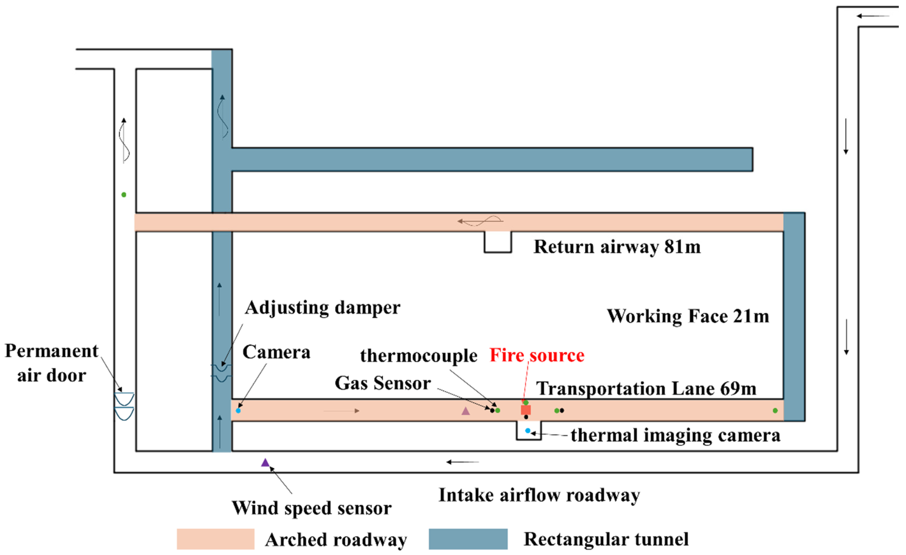
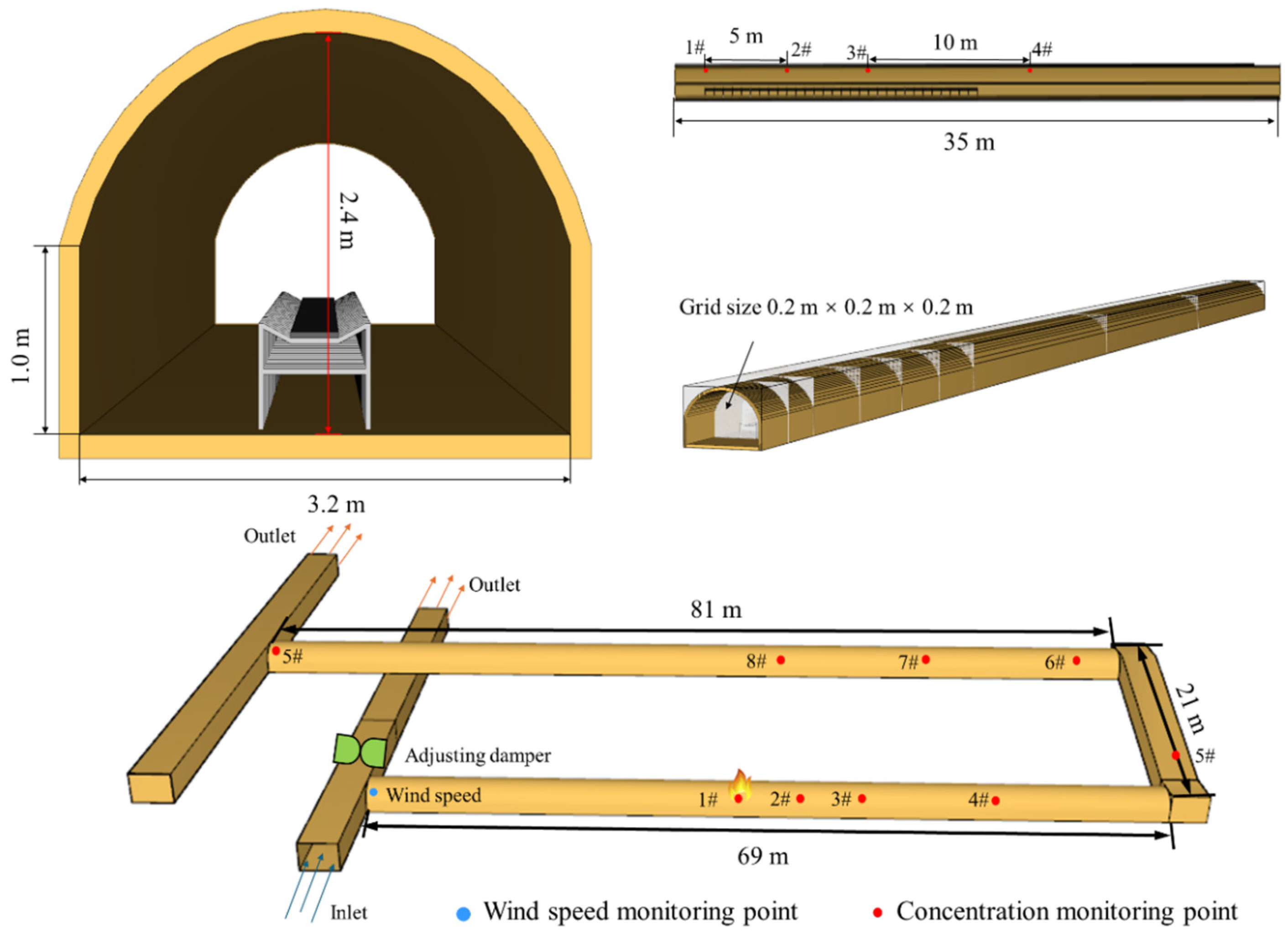
The experiments were conducted in the experimental roadway of the National Mine Emergency Rescue Kailuan Team in Tangshan, Hebei Province. Figure 4 illustrates the overall structure of the roadway; all sections are arch-shaped except for those marked as rectangular cross-sections.

The main conveyor belt roadway is 69 m long, 2.4 m high, and 3.2 m wide. Its top is semi-circular with a radius of 1.6 m, and the bottom rectangular section is 0.8 m high. The overall structure and field layout of the intake airway, where the fire source was located, are shown in Figure 5.

In the experiments, the fire source was positioned 35 m from the intake of the conveyor roadway, centrally located within the tunnel. It was placed on a metal tray, elevated 50 cm by a metal stand. Anhydrous ethanol served as the ignition source, with a 180 cm × 60 cm × 1 cm (length × width × thickness) conveyor belt strip placed directly above it.

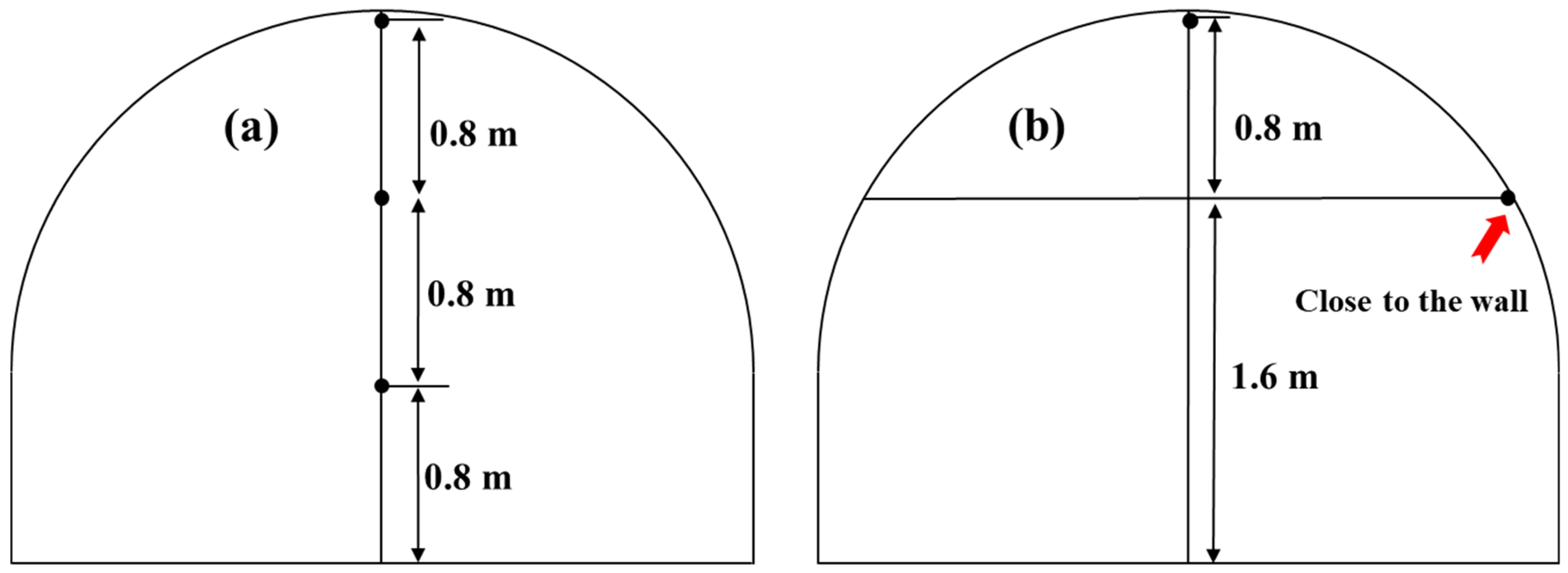
Thermocouples were strategically installed at the roadway ceiling and at heights of 0.8 m, 1.6 m, and 2.4 m above the ground. These placements included 5 m upstream of the fire source, at the fire source itself, and 5 m downstream of the fire source, as illustrated in Figure 6a.

A total of five sets of gas concentration sensors were deployed. Each set was capable of simultaneously measuring the volume fractions of CO and HCl. These sensors were located at 5 m upstream of the fire source, at the fire source, 5 m downstream of the fire source, 35 m downstream of the fire source, and at the end of the return airway. The arrangement of the gas concentration sensors is depicted in Figure 6b.

Wind speed sensors were positioned 4 m upstream of the three-way intersection in the intake airway and 15 m upstream of the fire source within the ignition experimental roadway. During the experiment, an HD camera was placed downstream and upstream of the fire source to observe the combustion state, while a thermal imaging camera was positioned 1 m to the right of the fire source to monitor changes in belt temperature.

The experimental roadway utilized a negative-pressure exhaust ventilation system. By controlling the operating frequency of the fan control box and using wind speed sensors located in the working face roadway and the main return airway, the corresponding air velocities in these sections were determined.

Gas concentration sensors (CO, HCl) as well as temperature and wind speed sensors are calibrated at multiple points before the experiment. The gas channel is linearly calibrated using standard mixed gases (CO and HCl concentrations of 2000 ppm and 200 ppm, respectively), the temperature channel is calibrated using multi-point thermocouples, and the wind speed channel is calibrated using a wind tunnel to ensure that the flow velocity reading error is less than ±0.05 m/s.

Six sets of full-scale belt conveyor fire experiments were conducted, covering three different wind speed conditions (0.2, 0.5 and 1.0 m/s). Each experiment lasted for about 1800 s, and the entire process from ignition to extinguishing was under stable ventilation conditions.

The experimental system is equipped with various types of sensors, including 12 gas concentration (CO, HCl), 9 temperature and 1 wind speed measurement points. The sampling frequency for wind speed, gas, and temperature was 1 Hz, resulting in 72 sets of gas concentration data.

2.7. Numerical Simulation

A numerical model was developed using Fire Dynamics Simulator (FDS), based on a full-scale fire experimental tunnel. Since underground horizontal roadways often have arched cross-sections, the curved structure of the roadway roof was modeled using a rectangular superposition method combined with the software’s smoothing function to minimize deviations in the simulation results.

The roadway walls were defined as 0.2 m thick concrete. The conveyor belt structure and dimensions were set according to actual mine specifications, with the framework made of metal steel and the belt material being Polyvinyl chloride (PVC). The combustion reaction parameters for PVC were redefined based on cone calorimeter experimental results and the PVC combustion reaction equation.

$${\left({\mathrm{CH}}_2-\mathrm{CHCl}\right)}_n+(5-\alpha )n/2{\mathrm{O}}_2\stackrel{\mathrm{Combustion}}{\to }2(1-\beta )n{\mathrm{CO}}_2+2\beta \mathrm{CO}+n{\mathrm{H}}_2\mathrm{O}+n\mathrm{HCl}$$

(21)

The initial ambient temperature for the simulations was set to 20 °C, with an initial pressure of 1 standard atmosphere. The intake airway wind speeds were varied at 0.5 m/s, 1.0 m/s, 2.0 m/s, and 4.0 m/s. Each simulation had a duration of 1800 s. Gravity acceleration was set to 9.81 m/s², and the pressure at both ends of the model was maintained at standard atmospheric pressure (1.01325 × 10⁵ Pa).

Along the axis of the conveyor belt, eight monitoring points were placed at 5 m intervals above the conveyor. The material’s heat release rate was configured based on the observed stages of the belt’s heat release rate during cone calorimeter experiments. Figure 7 illustrates the three-dimensional model of the conveyor roadway and the arrangement of monitoring points near the roof.

The numerical simulation part used FDS to establish the same geometric and wind field conditions as the experiment, and conducted three sets of simulations for six wind speed conditions of 0.2, 0.5, 1.0, 2.0, 3.0, and 4.0 m/s, with 16 monitoring points and a total of 288 sets of numerical simulation data.

3. Results and Discussion

3.1. Grid Sensitivity Analysis

Achieving more precise results necessitates a finer computational grid. However, this concurrently leads to a sharp increase in computation time. Therefore, balancing the accuracy of results with computational efficiency is crucial. As per the FDS User Guide, the ideal grid cell size should range between 0.0625D and 0.25D, where D represents the characteristic diameter of the fire source. This is calculated using the following equation:

$$D^{*}={\left({\displaystyle \frac{Q}{{\rho }_0{C}_P{T}_0\sqrt{g}}}\right)}^{{\displaystyle \frac{2}{5}}}$$

(22)

where Q is the heat release rate, ρ₀ is air density, C_P is the constant pressure specific heat capacity, T₀ is the ambient temperature, g is the gravitational acceleration.

Given the conveyor belt’s heat release rate and the fire source area, the maximum heat release rate in the FDS simulations was determined to be 900 kW. Consequently, the optimal grid cell size should fall within the range of 0.059 m to 0.261 m.

To test grid independence, a roadway fire with a heat release rate of 300 kW was simulated. Smoke temperature and HCl concentration at 0 m to 40 m downstream of the fire source were compared at a wind speed of 1.0 m/s and a time of 100 s, using grid sizes of 0.1 m, 0.15 m, 0.2 m, and 0.25 m, as shown in Figure 8.

Grid-sensitivity analysis showed that a 0.25 m mesh produced substantial deviations, whereas meshes of 0.10, 0.15, and 0.20 m yielded nearly identical smoke-temperature and velocity fields. Because the solution was effectively grid-independent at ≤0.20 m, a 0.20 m mesh was adopted to balance accuracy with computational cost.

3.2. Model Accuracy Validation

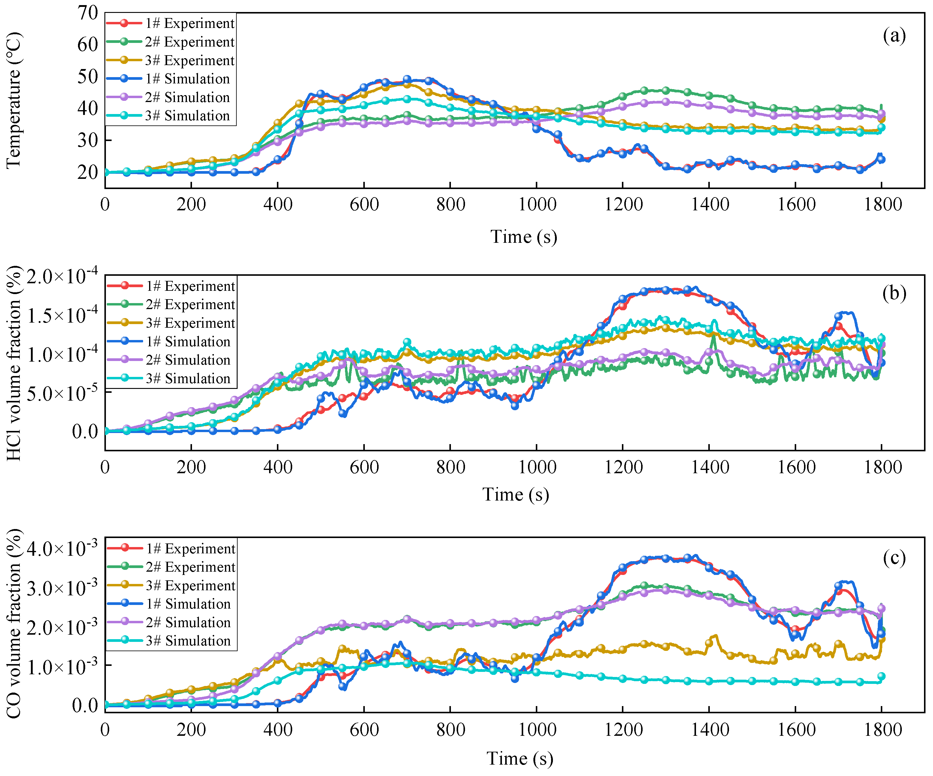
To validate the accuracy of the fire simulation results, temperature and HCl concentration changes at monitoring points 1#, 2#, and 3# under a wind speed of 1.0 m/s were selected for verification. The experimental and simulated values were compared and analyzed. Figure 9 illustrates the curves of temperature and HCl concentration changes at monitoring points 1#, 2#, and 3# during the fire simulation.

From Figure 9, it can be seen that the measured values of temperature and HCl concentration at monitoring points 1#, 2#, and 3# are basically consistent with the simulated values. Therefore, it can be considered that the calculation results of the tunnel flow field in the fire simulation are reliable.

3.3. Hyperparameter Tuning and Sensitivity Analysis

Table 2. Optimal hyperparameter values for PINN-LSTM gas concentration prediction model.

Type	Hyperparameter	Optimum
LSTM	Batch	112
	Hidden dimension	64
	Learning rate	1 × 10−4
	λ	0.9
PINN	Gas generation rate/kg s−1	1 × 10−3
	Effective diffusion coefficient/m2 s−1	1 × 10−5

summarizes the best predictive performance hyperparameters of the model.

A sensitivity analysis, conducted during the optimization process to identify the importance of hyperparameters, revealed that Learning rate scored the highest (30%), followed by Batch (30%), Hidden dimension (15%), λ (15%), Gas generation rate (5%), and Effective diffusion coefficient (5%).

Figure 10 shows the model’s validation error across different hyperparameters. The model performed better with a low validation error when λ > 0.5 and Learning rate < 0.01. By adjusting λ, it was verified that the loss gradually decreased with increasing λ, and the RMSE of the model decreased by 15%, significantly improving the predictive performance. This indicates that the original setting underestimated the fast advection constraint.

The Batch and Hidden dimension hyperparameters, however, exhibited optimal ranges of 96–128 and 32–64, respectively; values outside these ranges reduced model performance.

Validation error decreased as the gas-generation rate increased within the explored range, indicating a negative correlation and yielding more accurate gas-concentration predictions. By contrast, the effective diffusion coefficient showed a positive association with validation error: larger values produced higher errors and degraded performance. These trends are sensitivity-dominant hyperparameters that must be jointly tuned; empirically, increasing while constraining to moderate values most consistently reduced error.

3.4. Domain Generalization Test

To verify the generalization ability of the PINN-LSTM model in different data domains (numerical simulation and real experiments) and different operating conditions, this paper further designed three cross-domain and cross-scenario testing schemes based on the original data.

(1) Domain shift test

Train the model using all numerical simulation data and use actual experimental data as an independent test set to evaluate the model’s ability to transfer from numerical simulation to real data. Train the model using all experimental data and use simulated data as the test set to verify whether the model can generalize from real data to numerical simulation data.

Table 3. Cross-domain generalization performance of the PINN-LSTM model between different data domains.

	MSE	RMSE	R2
Train on FDS → test on experiments	9.56 × 10−5	2.76 × 10−5	0.97
train on experiments → test on FDS	9.26 × 10−5	6.58 × 10−5	0.95

shows the prediction errors (MSE, RMSE) and correlation coefficients for simulated data training experimental data testing and experimental data training simulated data testing. Both directional tests use the same network structure and physical constraints to evaluate the cross-domain robustness of the model by comparing prediction errors (MSE, RMSE) and correlation coefficients (R²).

According to Table 3, when the model was trained and tested on FDS data and experimental data, as well as on FDS simulation data, the R² across the two domains was not less than 0.95, indicating that the physical consistency constraint of the PINN-LSTM model played a key role in reducing inter-domain differences. The physics loss effectively prevented the model from overfitting to specific datasets across different distributions, thereby enhancing its generalization.

(2) Leave-One-Wind-Speed-Out

To verify the interpolation and extrapolation ability of the model under different ventilation conditions, three wind speed conditions (0.5, 2.0, and 4.0 m/s) were used as independent test sets, and the remaining three wind speed data were used for training to test the physical consistency and generalization performance of the model under wind speed changes.

As shown in

Table 4. Prediction performance of the PINN-LSTM model under different wind speed conditions.

Wind Speed (m s−1)	MSE	RMSE	R2
0.5	8.72 × 10−5	2.95 × 10−5	0.98
2.0	1.03 × 10−4	3.41 × 10−5	0.94
4.0	1.21 × 10−4	4.12 × 10−5	0.92

, as the wind speed increases from 0.5 m/s to 4.0 m/s, the model prediction errors (MSE and RMSE) show an upward trend, but the R² values remain above 0.90, indicating that the model has good prediction stability under different flow conditions. As the wind speed increases, turbulence intensifies and local mixing intensifies, resulting in more significant fluctuations in the concentration field and a slight increase in error. Overall, the PINN-LSTM model can maintain high accuracy under high wind speed disturbances, reflecting the strengthening effect of physical constraint mechanisms on generalization performance.

(3) Leave-One-Distance-Out

To further explore the spatial generalization ability of the model, the spatial positions (5, 20, 60 m) of the fire source distance sensor were set as independent test sets, and the remaining positions were used for training. This setting tests the transferability of the model under spatial feature changes, that is, whether it can accurately predict gas concentration at unknown distance positions.

According to

Table 5. Prediction performance of the PINN-LSTM model under different distances.

Distance (m)	MSE	RMSE	R2
5	7.85 × 10−5	2.80 × 10−5	0.96
20	8.06 × 10−5	3.61 × 10−5	0.95
40	9.13 × 10−5	3.90 × 10−5	0.93

, the performance difference in the PINN-LSTM model between different distances is relatively small (MSE increase < 20%, R² > 0.9), indicating its good spatial generalization ability. This stable performance is due to the introduction of physics loss in the loss function of the model, which not only relies on data-driven features, but also maintains cross spatial consistency by learning partial differential equation constraints.

The comprehensive results of the three types of tests show that the model has good out of domain generalization performance in the “FDS to experiment” direction, indicating that the physical constraint effectively alleviates the distribution difference between simulated and measured data; In the verification of wind speed and distance retention, PINN-LSTM can accurately capture the impact of wind speed changes on gas transport rate and concentration peak. This cross-domain and cross-scenario verification method ensures the generalizability and physical interpretability of the model.

3.5. Comparison of Ablation Experiment and Model Results

To further assess the contribution of physical constraints and model architecture, ablation experiments were conducted on three configurations:

(1) Removing the physics loss (pure LSTM);

(2) Removing the data loss on the PINN branch (physics-only model);

(3) Replacing LSTM with a Temporal Convolutional Network (PINN-TCN).

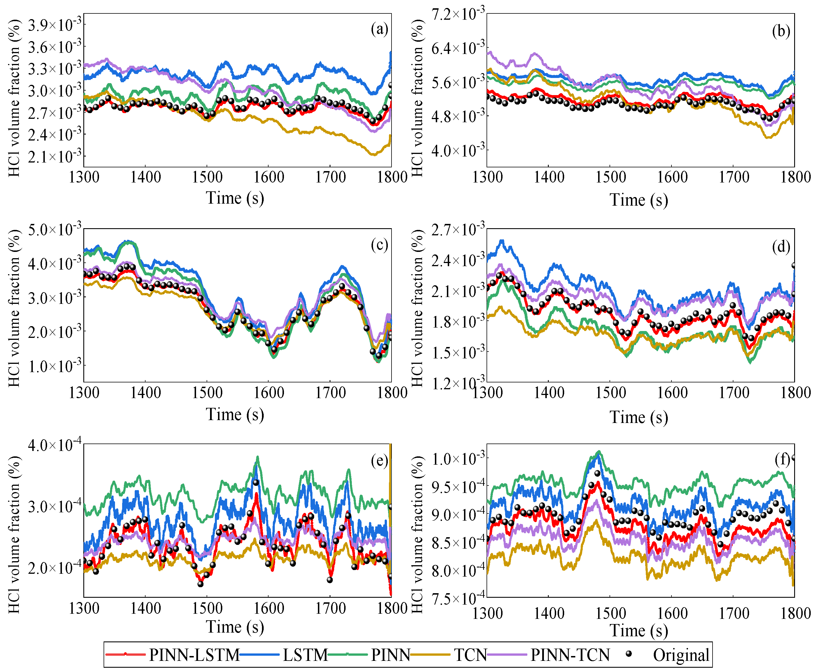
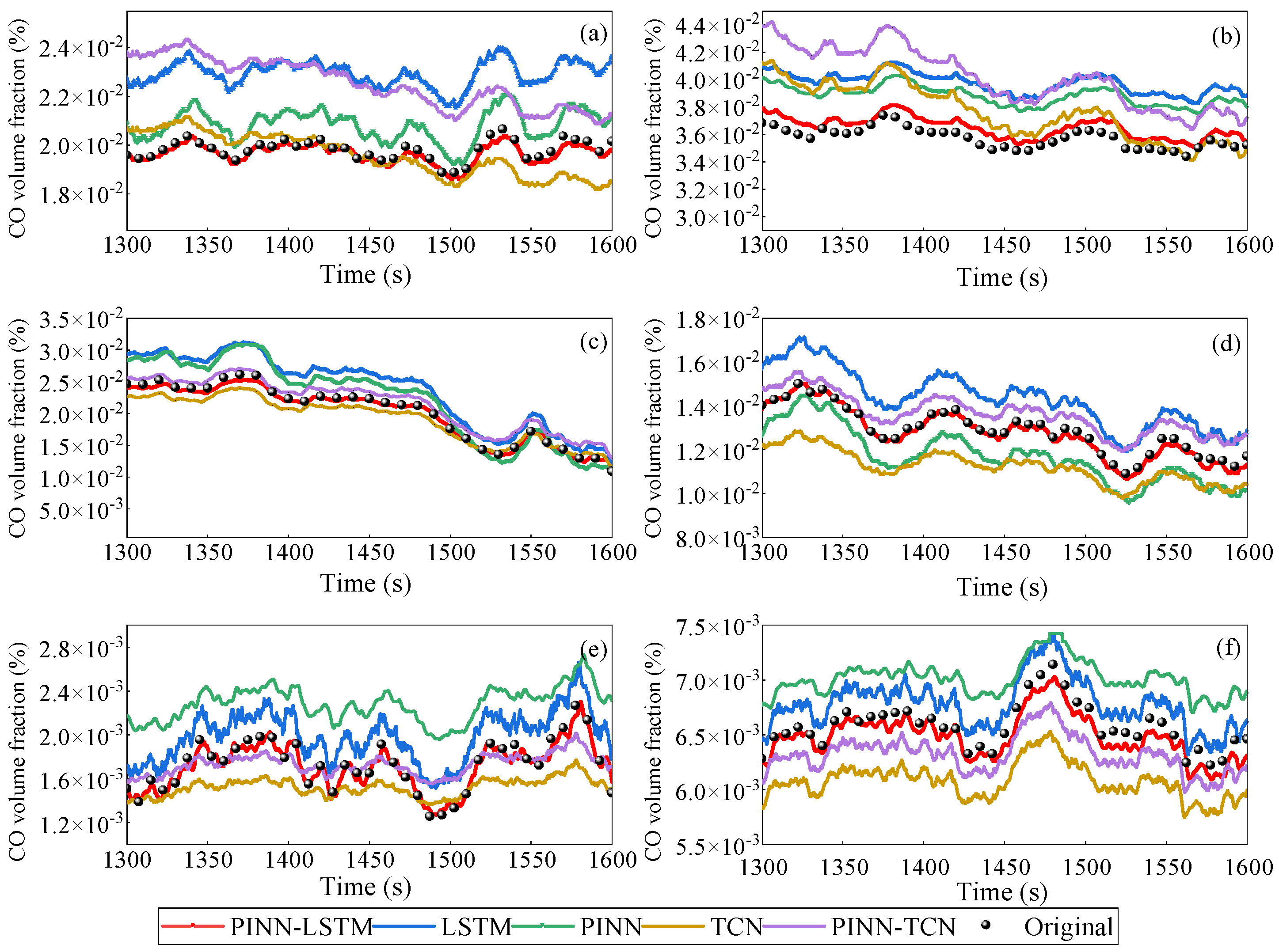
We explain the experimental results by comparing the PINN-LSTM model with three other prediction models. Figure 11, Figure 12 and Figure 13 show the raw data and gas concentration prediction results of five models at distances of 0 m, 5 m, 10 m, 20 m, 40 m, 60 m, 80 m, and 100 m from the fire source at a wind speed of 0.2 m/s. Figure 12 and Figure 14 show the raw data and gas concentration prediction results of three models at a distance of 5 m from the fire source at wind speeds of 0.2 m/s, 0.5 m/s, 1.0 m/s, 2.0 m/s, 3.0 m/s, and 4.0 m/s.

As shown in Figure 11 and Figure 13, the PINN-LSTM model consistently demonstrates lower error metrics than the LSTM, PINN, PINN-TCN and TCN models, indicating that integrating PINN with LSTM enhances generalization capability. The LSTM and PINN models exhibited similar performance, with the PINN model occasionally outperforming the LSTM. All models showed a tendency for error metrics to increase with greater distance from the fire source. Predictions closer to the fire source generally had lower error metrics and higher accuracy, a result of the increased complexity and irregularity of gas diffusion at greater distances.

Compared with PINN-TCN, the PINN-LSTM model exhibited slightly better accuracy and smoother temporal prediction profiles, with average MSE and RMSE values 8–12% lower across all distances. This advantage is attributed to the LSTM’s inherent ability to retain long-term sequential dependencies, allowing it to more effectively capture the gradual evolution of CO and HCl concentrations over time. Nevertheless, PINN-TCN also demonstrated strong stability and computational efficiency, verifying that the incorporation of physical constraints plays a more decisive role in improving model performance than the specific temporal network architecture.

As shown in

Table 6. Comparison of MSE and RMSE for predicting HCl volume fraction using models at different distances. (mean ± 95%, n = 10).

Model	Parameter	Distance (m)
		0	5	10	20	40	60	80	100
PINN-LSTM	MSE (×10−4)	0.31	0.25	0.31	0.33	0.30	0.36	0.41	0.55
	RMSE (×10−4)	0.38	0.39	0.40	0.40	0.38	0.40	0.48	0.71
LSTM	MSE (×10−4)	1.46	1.26	1.94	0.95	0.87	3.68	2.45	2.00
	RMSE (×10−4)	1.66	1.35	1.95	0.99	0.91	3.69	2.53	2.26
PINN	MSE (×10−4)	1.42	0.66	3.65	1.50	2.15	1.38	1.06	2.03
	RMSE (×10−4)	1.51	0.78	3.67	1.54	2.17	1.42	1.11	2.15
PINN-TCN	MSE (×10−4)	0.42	0.36	0.40	0.46	0.43	0.48	0.55	0.71
	RMSE (×10−4)	0.45	0.44	0.47	0.49	0.47	0.50	0.56	0.79
TCN	MSE (×10−4)	1.20	1.05	1.45	1.60	1.50	2.00	2.10	2.45
	RMSE (×10−4)	1.10	1.02	1.20	1.26	1.22	1.41	1.45	1.57

,

Table 7. Comparison of MSE and RMSE for predicting HCl volume fraction using models at different wind speeds. (mean ± 95%, n = 10).

Model	Parameter	Wind Speed (m/s)
		0.2	0.5	1.0	2.0	3.0	4.0
PINN-LSTM	MSE (×10−4)	0.25	1.03	0.66	0.34	1.06	2.17
	RMSE (×10−4)	0.39	1.11	0.78	0.42	1.08	2.19
LSTM	MSE (×10−4)	1.26	1.62	4.50	2.10	3.80	2.48
	RMSE (×10−4)	1.35	1.63	4.91	2.14	3.39	2.26
PINN	MSE (×10−4)	0.66	1.42	3.18	1.84	2.80	2.61
	RMSE (×10−4)	0.78	1.45	3.77	1.89	2.82	2.61
PINN-TCN	MSE (×10−4)	0.34	1.20	0.78	0.45	1.25	2.50
	RMSE (×10−4)	0.44	1.17	0.85	0.50	1.12	2.30
TCN	MSE (×10−4)	1.50	2.20	4.92	2.41	4.13	3.91
	RMSE (×10−4)	1.23	1.48	2.21	1.55	2.04	2.77

,

Table 8. Comparison of MSE and RMSE for predicting CO volume fraction using models at different distances (mean ± 95%, n = 10).

Model	Parameter	Distance (m)
		0	5	10	20	40	60	80	100
PINN-LSTM	MSE (×10−3)	0.31	0.25	0.31	0.33	0.30	0.36	0.41	0.55
	RMSE (×10−3)	0.38	0.39	0.40	0.42	0.38	0.46	0.48	0.71
LSTM	MSE (×10−3)	1.55	1.47	1.50	1.53	1.58	1.63	1.69	1.84
	RMSE (×10−3)	1.49	1.46	1.47	1.49	1.50	11.53	1.57	1.65
PINN	MSE (×10−3)	1.48	1.41	1.45	1.50	1.52	1.57	1.64	1.76
	RMSE (×10−3)	1.44	1.42	1.43	1.45	1.46	1.48	1.52	1.60
PINN-TCN	MSE (×10−3)	0.40	0.33	0.38	0.43	0.40	0.56	0.58	0.68
	RMSE (×10−3)	0.43	0.42	0.45	0.47	0.45	0.48	0.53	0.77
TCN	MSE (×10−3)	1.40	1.10	1.55	1.62	1.51	1.95	2.21	2.35
	RMSE (×10−3)	1.18	1.05	1.25	1.28	1.24	1.37	1.43	2.14

and

Table 9. Comparison of MSE and RMSE for predicting CO volume fraction using models at different wind speeds (mean ± 95%, n = 10).

Model	Parameter	Wind Speed (m/s)
		0.2	0.5	1.0	2.0	3.0	4.0
PINN-LSTM	MSE (×10−3)	0.25	0.33	0.26	0.34	0.46	1.07
	RMSE (×10−3)	0.39	0.31	0.28	0.42	0.59	1.19
LSTM	MSE (×10−3)	2.42	2.32	1.92	1.55	1.35	1.48
	RMSE (×10−3)	2.45	2.15	0.83	1.56	1.16	2.20
PINN	MSE (×10−3)	1.68	2.25	0.85	1.48	2.28	2.40
	RMSE (×10−3)	1.63	2.12	0.82	1.53	2.11	2.25
PINN-TCN	MSE (×10−3)	1.53	2.38	0.75	0.41	0.82	1.30
	RMSE (×10−3)	1.43	2.15	0.81	0.46	1.12	1.28
TCN	MSE (×10−3)	1.45	1.10	0.70	0.83	0.66	1.28
	RMSE (×10−3)	1.25	1.45	0.72	0.75	0.52	1.67

, the PINN-LSTM model consistently demonstrates lower error metrics than both the LSTM and PINN models, indicating that integrating PINN with LSTM enhances generalization capability. The LSTM and PINN models exhibited similar performance, with the PINN model occasionally outperforming the LSTM. All models showed a tendency for error metrics to increase with greater distance from the fire source. Predictions closer to the fire source generally had lower error metrics and higher accuracy, a result of the increased complexity and irregularity of gas diffusion at greater distances.

When comparing results across different wind speeds, the PINN-LSTM model consistently outperformed both LSTM and PINN. This confirms the accuracy and reliability of PINN-LSTM’s predictions under various wind speed conditions. At wind speeds of 0.2 m/s and 0.5 m/s, PINN-LSTM’s predictions were noticeably closer to the raw data than those of the other models. PINN-LSTM exhibited consistent performance, whereas LSTM and PINN showed greater fluctuations in error metrics at different depths. While all models showed higher error metrics at 4 m/s, the PINN-LSTM model maintained its advantage.

The quantitative comparison across Table 6, Table 7, Table 8 and Table 9 validates the consistency of the reported improvements. The PINN-LSTM model achieved the lowest MSE and RMSE under all distance and wind-speed conditions, with MSE reductions of approximately 70–78% compared to LSTM and 50–55% compared to PINN, while RMSE decreased by 65–73%.

When compared with the PINN-TCN model, the proposed PINN-LSTM exhibited slightly better accuracy and stability, with an average MSE reduction of 8–12% and RMSE reduction of 6–10%. This indicates that while both architectures benefit from the incorporation of physical constraints, the LSTM’s sequential memory structure provides superior capability in capturing long-term temporal dependencies of gas concentration evolution.

In contrast, the TCN model—lacking physical constraints—showed significantly higher MSE and greater fluctuation across different distances and wind speeds, particularly under strong turbulence (≥3 m/s). These findings demonstrate that the performance improvement of PINN-LSTM arises mainly from the integration of the physics-based convection–diffusion constraint, while the choice of temporal backbone (LSTM vs. TCN) contributes secondarily.

Overall, the PINN-LSTM model maintains the best trade-off between physical interpretability, predictive accuracy, and generalization, confirming its superiority for real-time gas concentration prediction in underground fire scenarios.

3.6. Uncertainty Quantification for Alarm Reliability

In the gas concentration prediction task of mine belt conveyor fires, the uncertainty of model prediction values directly affects the reliability of the alarm system. To this end, an uncertainty quantification mechanism was introduced in the output of the PINN-LSTM model to evaluate the confidence range and potential alarm error of the model’s prediction results.

To quantitatively evaluate the confidence interval of the model output, the Monte Carlo Dropout technique was used. Monte Carlo Dropout activation (dropout rate 0.1) during the prediction phase independently infers the same input sample 10 times and obtain the prediction set:

$$\left\{C_{pred}^{(1)},C_{pred}^{(2)},C_{pred}^{(3)}\cdots ,C_{pred}^{(N)}\right\}$$

(23)

Calculate mean and standard deviation:

$$\begin{array}{cc}\mu ={\displaystyle \frac{1}{N}}{\displaystyle \sum _i{C}_{pred}^{(i)},}& \sigma =\sqrt{{\displaystyle \frac{1}{N}}{\displaystyle \sum _i(C_{pred}^{(i)}-\mu }{)}^2}\end{array}$$

(24)

where σ is the uncertainty intensity of model prediction.

Calculate the 95% confidence interval for each time t:

$$C{I}_{95\%}(t)=\mu (t)\pm 1.96\sigma (t)$$

(25)

When the measured concentration C_true(t) exceeds the confidence interval, it is defined as a “high-risk prediction event”. The distribution of uncertainty over time shows that during the initial stage of the fire source and the sudden change in wind speed, the average σ of the model increases by about 45%, corresponding to the perceived instability of the model towards non-stationary convection diffusion.

In the mine monitoring system, the alarm threshold is usually based on the concentration of CO or HCl exceeding the set limit. Due to the uncertainty of model predictions, to avoid false alarms or missed alarms, the following risk indicators are defined:

$$R_{alarm}=P\left(\left|C_{pred}-C_{true}\right|>\delta \left|C_{pred}\approx C_{th}\right.\right)$$

(26)

where δ is alarm tolerance error, Cth is alarm threshold.

The statistical results show that under low to medium wind speed conditions, the alarm confidence level (1-Ralarm) of the model is higher than 0.93; at high wind speeds of 3.0–4.0 m/s, due to increased turbulence disturbance, the alarm confidence decreases to approximately 0.85. By combining uncertainty estimation, the system can trigger a ‘pre-alert state’ when the predicted confidence level is below a threshold, thereby reducing the risk of false alarms in actual operation.

The quantification of uncertainty provides a credibility boundary for the model output, allowing the predicted results to not only provide “concentration values” but also reflect “confidence levels”. This provides a more explanatory and risk-controllable decision-making basis for the intelligent alarm system for mine fires.

4. Conclusions

This study introduces a PINN-LSTM hybrid methodology, which integrates the strengths of both PINN and LSTM models, significantly enhancing prediction accuracy and robustness. The reliability and accuracy of the PINN-LSTM hybrid model’s predictions for precise gas concentration forecasting during mine conveyor belt fires were validated by comparing its results with data from full-scale roadway conveyor belt combustion experiments and numerical simulations. The main contributions of this research are summarized as follows:

(1) We developed a PINN-LSTM hybrid model suitable for predicting gas concentrations in conveyor belt fires. Model prediction accuracy was improved by optimizing training parameters through comparison of model training errors under various hyperparameters.

(2) We conducted full-scale roadway conveyor belt combustion experiments to monitor real-time gas concentration variations. Corresponding numerical simulations of conveyor belt combustion were performed based on these experimental conditions, with both experimental and simulation data collected to form the model’s training dataset.

(3) Cross-validation between FDS simulations and experimental data verified that the PINN-LSTM model maintained stable performance across domains. Additionally, Leave-One-Wind-Speed-Out and Leave-One-Distance-Out experiments confirmed that the model retained high accuracy and robustness under unknown wind speeds and spatial configurations, demonstrating strong interpolation and extrapolation capability.

(4) Ablation studies demonstrated that removing the physics loss increased MSE by approximately 72.8%, while removing the data loss on the PINN branch raised MSE by 54.3%. Comparative experiments with PINN-TCN and TCN models showed that PINN-LSTM outperformed both by 8–12% in MSE. The inclusion of physical constraints, rather than the network type, was the dominant factor driving accuracy improvement.