Abstract
This article presents a spatiotemporal super-resolution (SR) reconstruction model for two common flame types, a swirling and then a jet flame, using double generative adversarial network (GAN) architectures. The approach develops two sets of generator and discriminator networks to learn topographic and temporal features and infer high spatiotemporal resolution turbulent flame structure from supplied low-resolution counterparts at two time points. In this work, numerically simulated 3D turbulent swirling and jet flame structures were used as training data to update the model parameters of the GAN networks. The effectiveness of our model was then thoroughly evaluated in comparison to other traditional interpolation methods. An upscaling factor of 2 in space, which corresponded to an 8-fold increase in the total voxel number and a double time frame acceleration, was used to verify the model’s ability on a swirling flame. The results demonstrate that the assessment metrics, peak signal-to-noise ratio (PSNR), overall error (ER), and structural similarity index (SSIM), with average values of 35.27 dB, 1.7%, and 0.985, respectively, in the spatiotemporal SR results, can reach acceptable accuracy. As a second verification to highlight the present model’s potential universal applicability to flame data of diverse types and shapes, we applied the model to a turbulent jet flame and had equal success. This work provides a different method for acquiring high-resolution 3D structure and further boosting repeat rate, demonstrating the potential of deep learning technology for combustion diagnosis.
1. Introduction
To better understand turbulent combustion and develop new combustion models, three-dimensional (3D) diagnostics, which can resolve flame information in all three spatial directions, are necessary [1,2,3]. Real 3D measurements are now possible thanks to recent rapid advancements in scanning-based 3D imaging and computed tomography (CT). The preceding method scans a probe laser in a sequence of spatial locations and uses images captured at each site to create volumetric structures [4,5,6,7,8,9]. This scanning-based technique often calls for a laser with a high repetition rate, and instantaneity is always a challenge. Moreover, the spatial resolution along the scanning direction is typically much worse than that along the other two directions. Alternatively, the CT-based 3D imaging reconstructs the volume information of the flame using multiple perspectives. It has several adaptations, including volumetric laser-induced fluorescence (VLIF) [3], computed tomographic chemiluminescence (CTC) [10], 3D back-oriented schlieren [11], acoustic tomography [12], and others, and is now gradually becoming a well-established technology. In addition to being able to measure qualitative features, tomographic measurement has also been shown to be able to acquire quantitative information, such as temperature [13], soot volume fraction [14], and curvature [15]. Though its measurement can realize full dimensionality, CT imaging is typically constrained by the stiff barriers of limited view perspectives and computing resources. To be more precise, increased reconstruction resolution and accuracy is typically obtained experimentally by utilizing more 2D line-of-sight integrated projections from cameras or probes [11], but this is followed by higher experimental and computational costs. For instance, doubling the spatial resolution in 3D would require eight times as many cameras or probes [16], which is typically problematic for actual measurements. More severely, the number of views that can be added is even limited in a space-confined scenario [17,18].
In addition to aiming for complete spatial dimensions, time enhancement is another priority. Understanding the interaction of chemical reaction with turbulent flow, especially in high-speed propulsion systems, requires temporally resolving the flame structure due to the combustion field’s extremely dynamic change [19,20,21,22]. In-depth analysis of turbulent flow and chemical reactions helps to understand the combustion performance and emission characteristics of different fuels. For instance, De Poures et al. created four fuel mixtures by adjusting the SO concentration from 10% to 40% by volume. They then studied the emission characteristics in combination with the impact of hydrogen induction on compression-ignition engines [23,24]. Ü. Ağbulut et al. added nanoparticles to a mixture of fish oil and diesel, studying the performance and emission characteristics of engines fueled by this mixture [25]. Many high-repetition rate measures have been used to the field of combustion diagnostics as a result of the development of hardware devices, such as high-speed cameras, burst-mode lasers, and intensifiers [26,27,28]. Due to the hardware system’s restricted repetition rate, limited laser pulse energy, and the challenges associated with storing and distributing huge data, further improving image quality is extremely tough, which forces us to choose between spatiotemporal resolution and imaging accuracy [8]. However, the cost of investing in lasers and cameras is substantially higher, particularly for systems with high repetition rates. In these conditions, a learning-based super-resolution (SR) technique that strives to enhance both the spatial and temporal resolution of combustion measurements with a particular experimental setup is highly desirable.
SR is a successful method that is frequently applied in a variety of disciplines, including microscopy, satellite surveillance, computer vision, and others. SR has been proven to work in both 2D and 3D space, in the space and time domain, and in reacting and non-reacting flows in a more limited range of turbulent flow and combustions. In the early days of 2D SR, the SR problem was treated as an inverse problem of upscaling the low resolution (LR) images to generate a high-resolution (HR) image with additional features, which are fundamentally unknown. The kernel-based SR reconstruction of 2D images has been investigated for decades. Convolutional neural network layers have been used more recently in learning-based SR techniques to learn the features of the images and rebuild the HR with perceptual information. A detailed analysis of the application of machine learning to turbulent flows must be performed, nevertheless considering the intricate spatial structures of extremely turbulent flows. For instance, Xu et al. applied deep learning to combustion diagnosis by using a GAN to predict the HR structure of a 3D flame field [16]. Cheng et al. used a GAN to predict 2D smoke signals. By inputting the luminosity projection of jet flames, they were able to reconstruct the 3D distribution of smoke particles, providing new insights into the formation and distribution of smoke [29]. Zhang et al. report a computational method based on deep learning (DL) to generate planar distributions of soot particles in turbulent flames from line-of-sight luminosity images [30]. Anthony Carreon et al. applied GAN to generate realistic flame images based on a time-resolved dataset of hydroxide concentration snapshots obtained from planar-laser-induced fluorescence measurements of a model combustor [31]. Fukami et al. reported machine-learning-based spatiotemporal super-resolution reconstruction of 2D isotropic turbulence and 3D channel flow [32]. Dong et al. achieved temporal interpolation using computational imaging by artificially generating sequential OH PLIF images at 200 kHz based on 100 kHz and accelerating the high-speed planar imaging of turbulent flames with a convolutional long short-term memory network [33,34]. Similar applications of the machine learning models in a variety of flow reconstructions are inspired by these earlier works based on data reconstruction using these models [35,36,37], which moderately overcome environments in which only partial or low-resolution spatiotemporal data are available due to the limitations of measurement equipment or computational resources. Nevertheless, to the authors’ knowledge, the spatiotemporal SR imaging in the 3D combustion field has not been reported.
Therefore, the goal of this work is to explore the feasibility of using a learning-based model to improve the spatiotemporal resolution of 3D turbulent flames. High spatiotemporal resolution sequences are predicted using input sequences of 3D turbulent flame structure, yielding resolution increase in both space and time. The following presents and discusses the network model’s specifics, the method of data training and prediction, and the evaluation of model accuracy.
2. Materials and Methods
2.1. Turbulent Flame Data
The training data are a necessary component and prerequisite for subsequent network modeling. In this study, large eddy simulation (LES) is used to provide the 3D volumetric flame data of a swirling flame and a piloted turbulent jet flame. These two types of flame were chosen based on two considerations. First, these two flames have been widely studied, and published references can be found. Second, these two types of flame cover a wide range of flow phenomena that are of particular interest for the combustion community, such as mixing, high turbulence, and local extinction. The swirling flame uses the burner geometry according to the data repository [38], which consists of a burner base with a 25 mm diameter conical bluff-body and a 37 mm annulus with a swirler upstream. The geometric swirler upstream of the bluff-body consists of six vanes at 60° with respect to the flow axis. Four quartz plates are supported by the burner body, forming a square combustion chamber, 97 mm wide and 150 mm tall. The outlet is open to the atmosphere, and the direction of the air swirl is clockwise when looking at the nozzle from the combustion region. The boundary conditions were set to generate a low velocity swirl flame without too much blow-off. The bulk velocity of the flow at the air inlet was set to 10.73 m/s, according to reference [39], and the methane fuel velocity was set to 38.6 m/s. Under such a configuration, the overall equivalence ratio was 0.45. To avoid overly focusing on mesh production and considering the geometric complexity, a hybrid mesh that has an unstructured grid for the swirler and a structured grid for the flame chamber was constructed for computation. The half cone angle of the CH4 fuel injection into the combustion chamber was 30 degrees. The governing equations were reactive Navier–Stokes equations that were solved using the finite volume approach while taking into account a 16-component skeletal chemical reaction mechanism between CH4 and air. The eddy dissipation concept (EDC), which assumes that molecule mixing and the subsequent combustion occur at fine scales, was employed to account for the turbulence–chemistry interaction in the simulation. The Smagorinsky–Lily sub-grid scale model was used to close the control equations. Flame data were saved every 25 time steps, and the incremental time step used in the LES simulation was 1.0 × 10⁻⁵ s, which was tiny enough to capture the dynamic features of the flame.
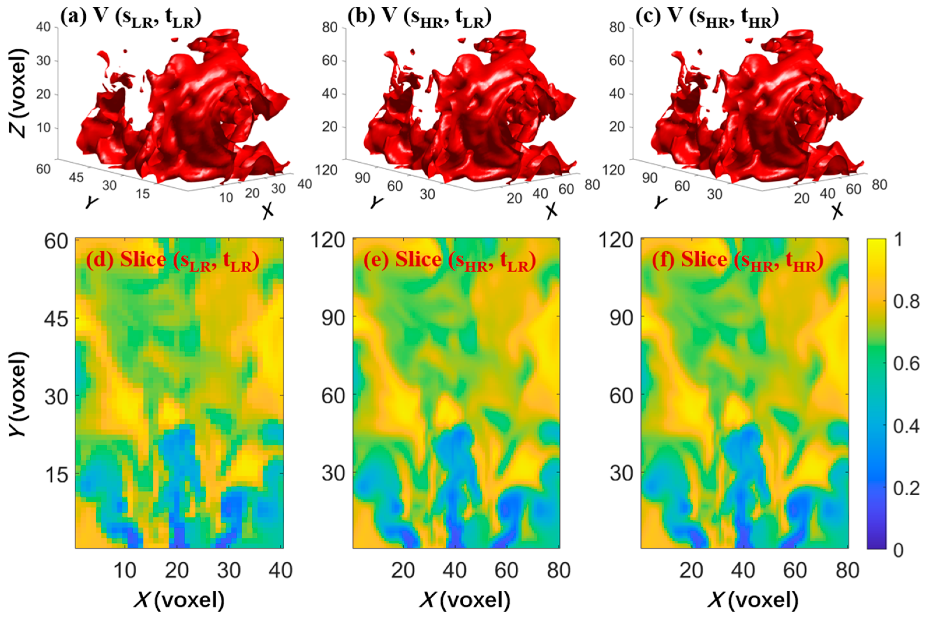
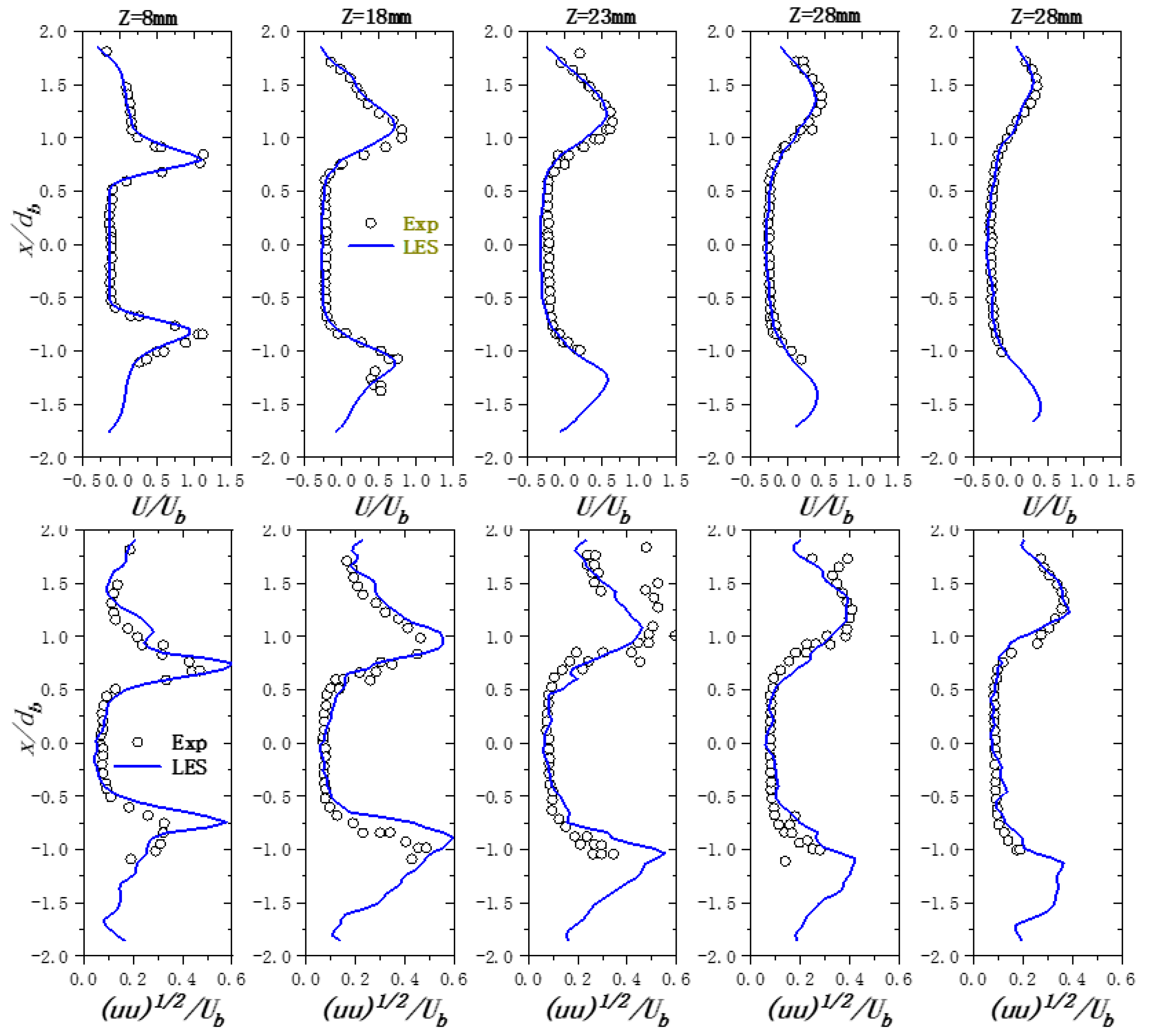
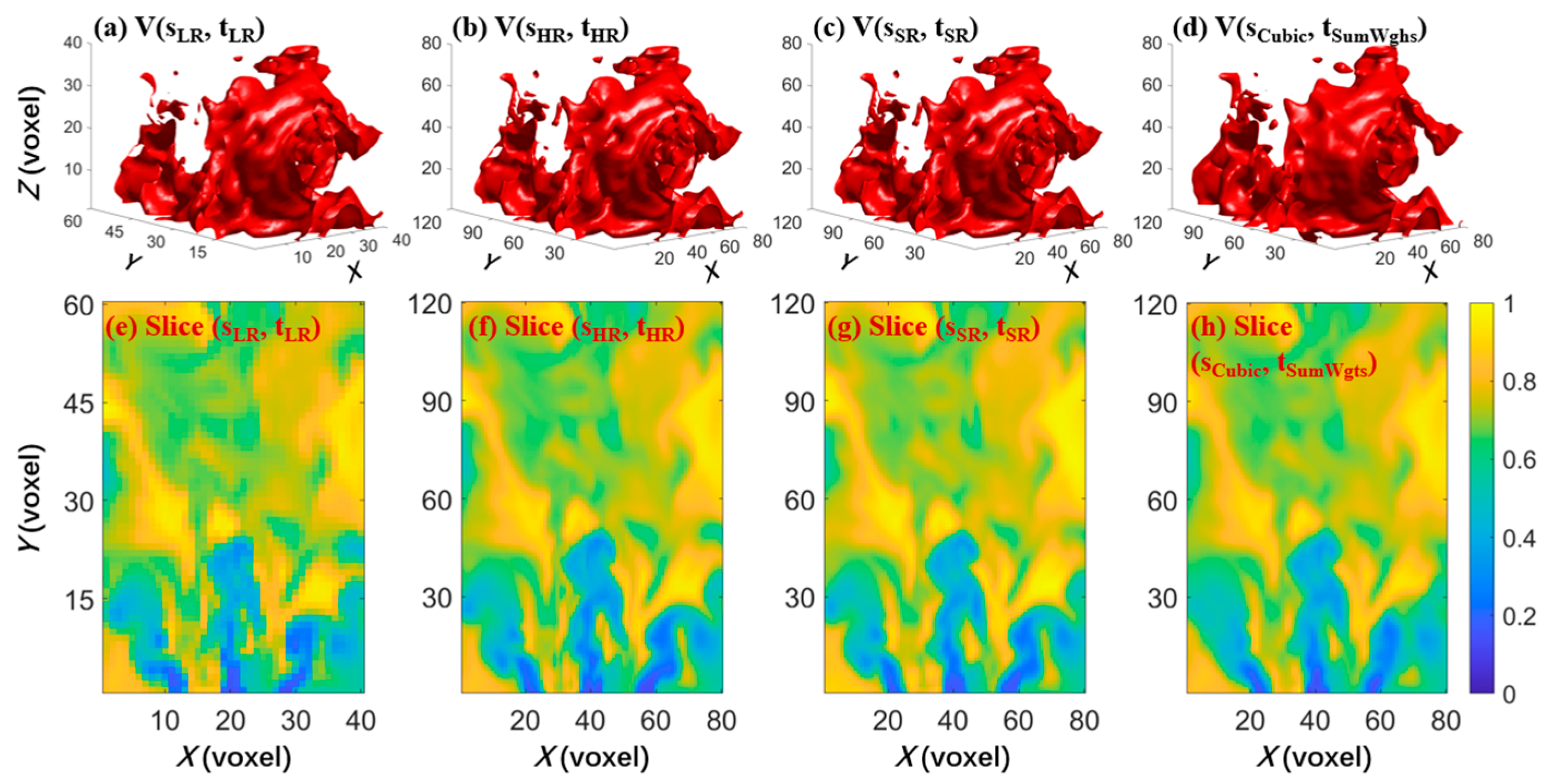
The objective of this work was to reconstruct a SR flame field, V(, ), from low-resolution (LR) data, V(, ). Figure 1a–c displays the 3D flame data. Figure 1a,c are essentially the input and target of the SR model, while Figure 1b represents the intermediate product, V(, ), with HR in space and LR in time. To better illustrate the difference in flame data at different resolutions, Figure 1d–f show the 2D central slice of Figure 1a–c. Obviously, the HR data of 120 × 80 × 80 were visually clearer than the LR data of 60 × 40 × 40, including more field textures and finer flow details, while the LR data somehow missed some high-frequency information. The HR flame had a nominal spatial resolution of 1 mm, compared to 2 mm for LR data. During the large eddy simulation (LES) sampling process, by setting the time step length and halving the time step for each frame, high temporal resolution flame data can be obtained relative to the low temporal resolution flame data, thereby achieving a twofold enhancement in the temporal SR of the flame. The simulated flame data were split into two halves as the training dataset, of which 400 snapshots were utilized to update network parameters during training and the remaining 40 snapshots were used to assess the performance of the trained network. Due to the periodicity of the swirling flame field, it should be noted that the nature of the training and test datasets are comparable to one another. The reason for not setting a validation dataset is that the flame structure with the same Reynolds number should obey the same distribution in latent learning space so that there is no substantial effect. The LES simulation of the swirl flow is believed to be reasonable, according to the comparison against experimentally acquired RMS axial velocity, as shown in Figure 2. The experimental data points were adopted from the published paper from reference [39]. Good agreements of both mean and RMS of the axial velocity, not only in the near region from the bluff body but also downstream, validates the accuracy of the LES simulation. Moreover, the motivation of this paper originated from limited spatiotemporal resolutions in volumetric tomographic measurements, and the focus of this work lies in the demonstration of a well-designed GAN architecture that can boost both spatial and temporal resolution of a turbulent flame. The main role of the LES simulation is providing the training data, which have resolved the geometric and intermediate length scale and sufficiently small time scale. It is noted that the spatial resolution of the state-of-the-art tomographic measurement is still far away from that of numerical simulation.
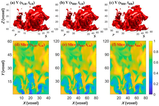
Figure 1.
Presentation of simulation data: (a–c) isosurface rendering of 3D swirl flame; (d–f) 2D central slice.
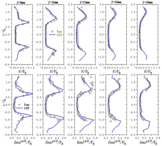
Figure 2.
Mean and RMS velocity comparison of LES simulation in this work and experimental data [39] of the swirl flame at different stations at the indicated distance from the bluff-body.
As the turbulent jet flame has been extensively discussed in the literature [40,41,42,43], only a brief explanation of it is given here. The main jet nozzle had an inner diameter of 7.2 × 10⁻³ m, and the bulk velocity of the central jet flow was 29.7 m/s, which resulted in a jet Reynolds number of 1.34 × 10⁴. The boundary conditions for the main jet, pilot flame, and coflow were set according to the experimental measurement [42], which corresponds to a Sandia Flame C configuration. The increment time step was set to 1 × 10⁻⁵ s, which was sufficiently small to capture the flame’s dynamic properties. In order to conduct the spatial and temporal SR analysis, we typically utilize 600 training datasets. In this example, we used 40 test snapshots, aside from the training data, for all evaluations.
2.2. Spatiotemporal SR Model
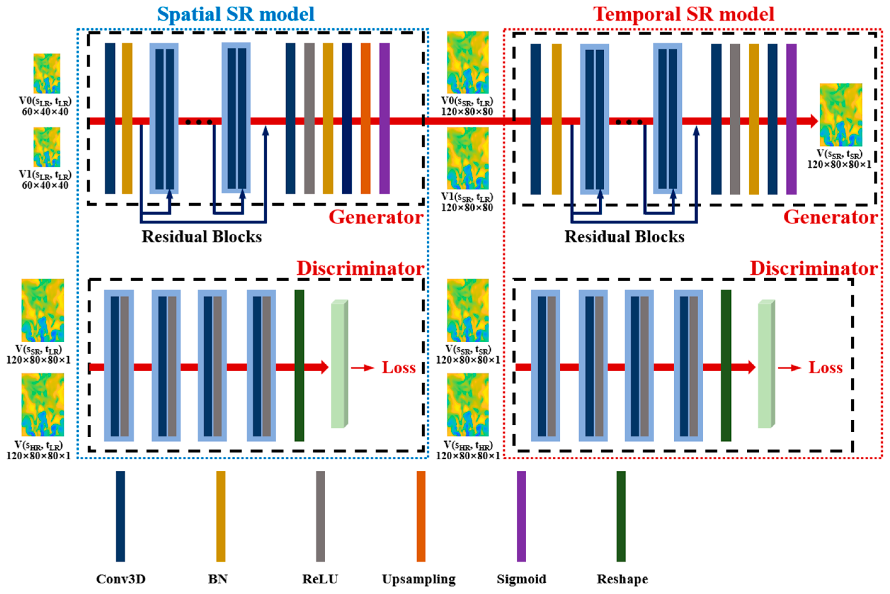
To achieve the goal of reconstructing the SR flame field, V (, ), from the LR data, V(, ), we combined spatial SR analysis with temporal inbetweening to establish the deep learning model for 3D spatiotemporal SR, as illustrated in Figure 3. Initial SR operation was designed to reconstruct spatially SR data from input data (for swirling flames: LR at 60 × 40 × 40 and SR at 120 × 80 × 80), achieving an eightfold enhancement of the total voxel number, as shown on the left half of Figure 3. The successive temporal SR was aimed at finding the intermediate frame based on the previous spatial SR results of the head and tail frames, as shown in the right half of Figure 3. Both the spatial and temporal SR models are based on GAN architecture that consists of a generator and a discriminator. Both spatial reconstruction and temporal reconstruction consist of two main components: the generator model G and the discriminator model D. The generator model reads the 3D structure with low spatiotemporal resolution and outputs the reconstructed version, while the discriminator model evaluates the reconstruction results produced by the generator based on the original 3D flame structure. The training process of the 3D spatiotemporal SR reconstruction network is essentially an optimization problem of the loss function defined by it, under the condition of a given training dataset. For the generator, the purpose of the training process is to enable it to output spatiotemporal SR reconstruction results that are convincing enough to deceive the discriminator. The purpose of training the discriminator is to distinguish between the original high spatiotemporal resolution 3D structure and the reconstruction results of the generator. As the generator and discriminator networks are trained alternately, the network parameters are continuously updated, making the reconstruction results of the generator increasingly close to the original high spatiotemporal resolution 3D structure, until the discriminator can no longer distinguish between the two.
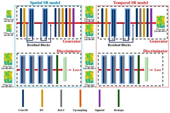
Figure 3.
Architecture of spatiotemporal super-resolution network for 3D flame reconstruction based on GAN.
Although these two processes are independent in the current model, we decided to conduct the spatial SR first and the temporal inbetweening afterwards. This was done to prevent the error between the reference data V(, ) and the test data V(, ) from accumulating during the temporal SR process. Otherwise, as the inbetweening using spatial LR data lacks very precise texture information, the disparity between pre-generated V(, ) and V(, ) would be magnified in following the spatial SR.
For the spatial SR model, we prepared a set of inputs, V(, ) and V(, ), as the training data to obtain the intermediate result, V(, ), which acts as input for the successive temporal SR model. The generator of the spatial SR model first reads the LR data V(, ) and upsamples it into spatial SR counterparts V(, ), while the discriminator of the spatial SR model judges the model-predicted spatial SR data, V(, ), from its counterpart, V(, ). As can be seen from Figure 3, each colored rectangle represents a specific operation. The size of the 3D convolutional kernel was fixed at 3 × 3 × 3, and the number of output channels and strides were set to 64 and 1, respectively, which represents a compromise between computing cost and model performance. For each convolution operation, a zero-padding operation was used to maintain the size of the input data. Moreover, we used a rectified linear unit (ReLU) as the activation function. The use of ReLU is known to be an effective tool for stabilizing the weight update in the machine learning process [44]. In particular, we extended the generator model by introducing skipped connections, as shown by the blue arrows in Figure 3. The use of skip connections can enhance the model’s learning capability by relieving convergence issues, which is known to be a problem with deep neural networks. The combination of skip connections and residual blocks helps avoid gradient dispersion and deepen the network without too much extra coding [45]. The detailed structure of the discriminator is also depicted in the lower part of Figure 3. The number of its output channels progressively increased from 4 to 64, allowing the discriminator to distinguish subtle differences between the model-predicted SR result and its ground-truth. Eventually, each discriminator outputs a long vector of 44,752,850 elements with a feature distribution of either model-predicted or ground-truth data.
As for the temporal inbetweening process, two spatial SR flame fields V(, ) outputted by the spatial SR model of head and tail frames are used as the input for the following temporal SR process, and the corresponding inbetweening snapshot would be reconstructed by the temporal SR model. Note that the architectures of the spatial and temporal SR processes are essentially the same, while the difference is mainly in the input. Similar to the spatial SR operation, the discriminator of the temporal SR model is used to judge the inbetweening result V(, ) from its counterpart V(, ). The former is used to distinguish the spatial SR results V(, ) from ground-truth volume data V(, ), while the latter is aimed at telling the inbetweening V(, ) from its real temporal counterpart V(, ).
During the training process of our proposed model, the final goal is to develop a mapping function that makes generator output fake volumes that are very close to their real counterparts so that the discriminators cannot distinguish them. From a mathematical perspective, the essence of network training is to minimize the loss functions, which reflect the difference between the model results and their real counterparts. Therefore, the design of the loss function is of great significance for neural network modeling. For the spatial generators in this work, the loss function is a combination of two loss terms, including mean square error loss, , and adversarial loss, .
The mean square error loss, , is defined in a voxel-by-voxel manner, as shown in Equation (2),
The adversarial loss, , calculates the cross-entropy between the output of the generator and the ground-truth data, representing the perceptual agreement and preventing the output results from being over-smoothed. The definition of is presented in Equation (3),
To keep the balance of convergence, the weight of the is set as = 1 × 10⁻³. The loss function of the discriminators is defined by the sum of two feature distributions for the output of the generator and its ground-truth counterpart, as shown in Equation (4):
Loss functions of the temporal SR have similar form as Equations (1)–(4), while the subscripts of the two need to be changed into and , respectively. The essential building blocks of the spatial and temporal networks are identical, and therefore little additional coding work is needed. It is noted that the ultimate configuration of the network architecture was obtained through fine tuning of the network parameters, as reported in previous papers [16,41]. The parameters that could be adjusted include depth of each convolutional layer, the number of residual blocks, and the use of activation function.
2.3. Convergence of the Spatiotemporal Model
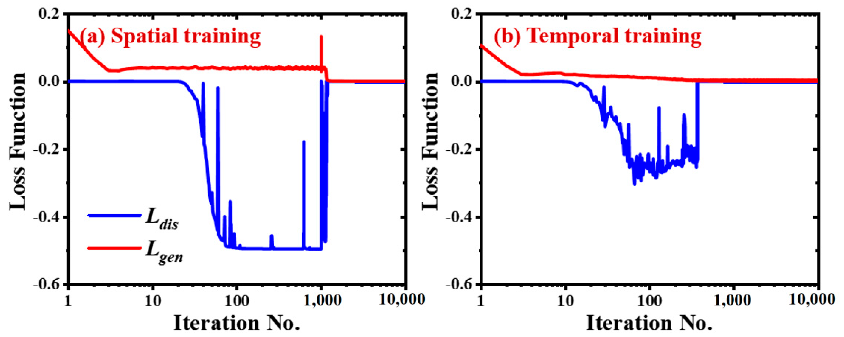
The goal of this work is to establish an input–output mapping relationship as soon as training begins so that the results predicted by the model can fool discriminators. When the predicted outcome of the generator is sufficiently similar to the associated ground truth that they can no longer be separated after alternately training generator and discriminator networks, the network has reached convergent status. The proposed spatiotemporal SR network is implemented using the TensorFlow framework, and the network is trained using two NVIDIA GEFORCE RTX 3090 GPUs. The learning rate was set to 0.001, and the initialization of the trainable parameters was done at random. When the iteration steps of the spatial and temporal training were set to 5000 and 10,000, respectively, it took this work ten hours of training to reach a convergent solution. The time needed for a pre-trained network model to forecast spatiotemporal SR data was roughly 20 milliseconds. In the training phase for the spatiotemporal SR network, Figure 4 depicts the evolution of the loss functions. It is obvious that the and had converged to zero for both the spatial and temporal training processes, indicating a successful reconstruction could be accomplished.
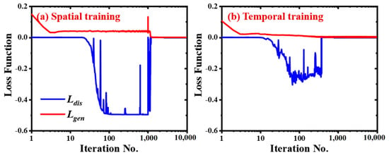
Figure 4.
Evolution of the loss functions for the training process: (a) loss function variation of spatial SR training and (b) loss function variation of temporal SR training.
3. Discussion and Results
3.1. Spatiotemporal SR Based on Swirling Flame
In order to clearly demonstrate the superiority of the network-predicted output, this section assesses the reconstruction performance of the 3D spatiotemporal SR network from both qualitative and quantitative perspectives and compares the findings with those of three direct interpolation methods. The three approaches for interpolation are closest [46], linear, and cubic [47,48]. The simplest of these techniques is the nearest interpolation, which uses the value of the closest location as the goal value after merely searching the neighborhood. The linear interpolation method involves calculating the weight coefficient depending on the distance from the adjacent voxel in order to obtain the voxel value. The weighted average value around the target region can also be calculated by the cubic interpolation using specified convolution kernels, which also allows for upsampling. In this work, a qualitative comparison refers to a visual comparison of the volumetric or planar flow structure of the model prediction. The planar comparison might give a more straightforward indication of agreement, while the volumetric comparison is used to confirm that the entire topographic corresponds. Peak signal-to-noise ratio (PSNR), reconstruction error (ER), and structural similarity (SSIM), all of which are metrics commonly used in the literature for picture evaluation, were employed for the quantitative comparison in this work. The PSNR is a metric for measuring image quality, which assesses the difference between the original image and the distorted image. Specifically, PSNR calculates the ratio of the peak pixel intensity to the average noise intensity. In image reconstruction, a higher PSNR indicates smaller differences between the reconstructed image and the original, signifying better image quality. PSNR values are typically expressed in decibels (dB), with higher values indicating image reconstruction quality closer to the original image [49], whereas the ER is a metric that measures the discrepancy between the reconstructed image and the original image. It calculates the square root of the sum of the squared errors across all pixel points, providing a comprehensive measure of error. A lower ER value indicates a higher consistency between the reconstructed image and the original, signifying better reconstruction results. ER is a straightforward quantitative indicator that helps assess the model’s performance in detail restoration [16], and the SSIM is a more complex image quality assessment metric that considers not only luminance and contrast but also the structural information of the image. SSIM compares the luminance, contrast, and structural information of the original and reconstructed images, calculating a value between −1 and 1, with values closer to 1 indicating greater similarity. SSIM is particularly suitable for evaluating visual image quality as it better reflects human perception of image quality [50]. In general, better reconstruction quality favors a higher PSNR, a smaller ER, and a larger SSIM. Higher PSNR indicates that the model can effectively recover image details, reduce noise, and provide clear image outputs. A smaller ER suggests that the model can accurately reproduce the information of the original image with minimal error during reconstruction. A larger SSIM implies that the model not only maintains consistency with the original image in terms of luminance and contrast but also highly resembles it in structure, which is crucial for capturing complex flame structures. These three indicators are introduced to explore the network performance from two perspectives, the initially generated spatial SR flame and the ultimate spatiotemporal inbetweening flame.
The outcomes of the interpolation methods were compared with the intermediate outputs produced by the spatial SR process as a first-stage evaluation, as shown in Figure 5a–c. A number of conclusions can be drawn from the figure. Due to the three interpolation algorithms’ various operating principles, the cubic interpolation came in first place. Second, among the four techniques, the proposed spatial SR model performed the best in terms of reconstruction. Lastly, the test dataset shows consistent reconstruction quality for the SR model and the three interpolation approaches, indicating a reliable and convincing model performance. Specifically, the cubic technique yielded 36.29 dB and 0.991, respectively, which is the optimal interpolation, compared to the mean values of 37.94 dB and 0.992 for the PSNR and SSIM of the spatial SR model. In terms of the mean ER, the spatial SR’s value of 1.2 percent was just marginally higher than the cubic method’s 1.21 percent. This indicates that the spatial SR process is effective enough to produce superb spatial reconstruction with an upscaling factor of 2, which can deliver a high-quality input for the subsequent operations of temporal SR.

Figure 5.
The quantitative comparison between our spatial SR model and three traditional interpolation methods, namely, nearest, linear, and cubic: (a) variation of PSNR; (b) variation of ER; (c) variation of SSIM.
As shown in Figure 6, based on the results of spatial reconstruction, new frames were reconstructed between each pair of adjacent frames in the sequence, achieving a twofold increase in the temporal resolution of the swirling flame. Figure 6a displays the slicing images of the swirling flame at two time frames (T0, T1), as well as the SR images of time based on the SR model and linear interpolation. It can be observed from the red square in the figure that the result of linear interpolation lost the small swirling flame structures. In contrast, the result from the SR model was more in line with the dynamic changes of the flame. Figure 6b shows a one-dimensional comparison of the results along the red dashed line, and it can similarly be observed that the result of the SR model had temporal extension, while the linear interpolation result was merely an average one, without temporal correlation.

Figure 6.
The comparison of temporal SR results of the SR model and linear interpolation. (a) Slicing images of the swirling flame at two time frames (T0, T1) and the SR images of time based on the SR model and linear interpolation. (b) One-dimensional comparison of the results at the red dashed line.
The quantitative comparison of our SR model with the conventional closest, linear, and cubic interpolation methods on the test dataset is presented in Figure 7a–c. It should be noted that the direct interpolation results in Figure 7 actually denote the corresponding spatial interpolation method, while the temporal interpolation was simply weight averaging based on time sequence. Taking the cubic results in Figure 7 as an example, it first conducted spatial interpolation using the cubic method and then calculated a weighted sum of two spatially upsampled frames with weight coefficients of 0.5. According to Figure 7, the cubic method was still the best among the three interpolation methods, with PSNR and SSIM mean values of 28.94 dB and 0.95, respectively. Comparatively, the PSNR and SSIM indices for the test performance of our model were 35.28 dB and 0.985, respectively. With regard to ER, it is evident that a mean value of 1.7% of inbetweening was significantly less than the cubic interpolation shown in Figure 7c. Therefore, our model outperformed direct interpolation in the spatial SR stage, and the superiority was even more prominent compared with the case of solely spatial SR. However, we cannot intuitively determine which is superior based only on these general evaluation measures; rather, more thorough and visual examples are required, as will be shown in the examples that follow.

Figure 7.
The quantitative comparison between temporal inbetweening and the result of three interpolation methods: (a) variation of PSNR; (b) variation of ER; (c) variation of SSIM.
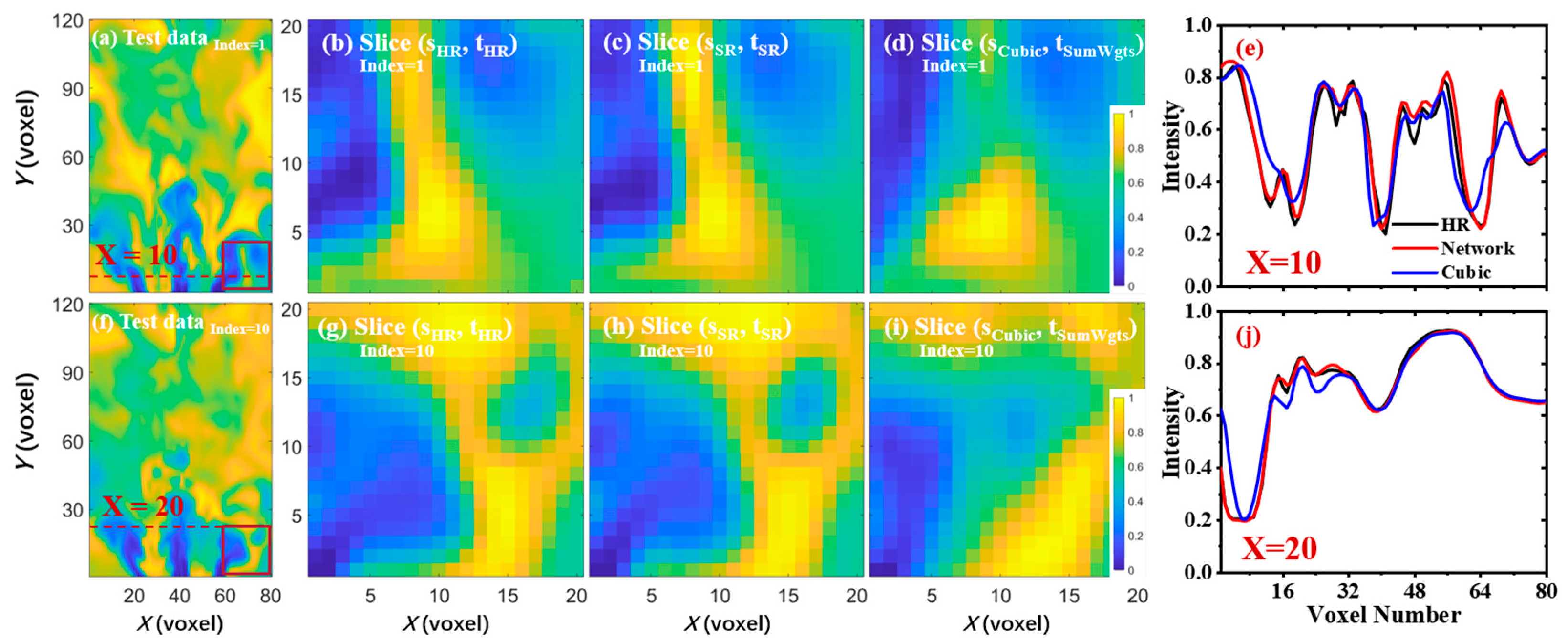
To better visualize the capability of our spatiotemporal SR network, Figure 8 and Figure 9 display the reconstructions effect by comparing the SR flames with ground truth flames from 3D, 2D, and 1D. Figure 8 shows the sole use of the cubic approach as the control group since, as was previously discussed, it is the best of the three interpolation methods provided. Figure 8a–d show a case of the 3D turbulent flame rending of the V(, ), V(, ), V(, ), and V(, ), respectively. Among the results, the V(, ) and V(, ) represent the LR resolution data and corresponding HR data, while the V(, ) and V(, ) are, respectively, the spatiotemporal SR results of our model and the cubic interpolation, which are eight times the voxel number of LR data and twice the time repetition rate. From Figure 8a–d, it can be found visually that both V(, ) and V(, ) are quite similar to V(, ). There seems to be some improvement with more flow texture compared with V(, ), but it is hardly noticeable. From this sense, a more localized visual examination is necessary. We then extracted 2D central slices with constant X coordinate from Figure 8a–d, as shown in Figure 8e–h. The 2D slice view clearly shows more intuitive comparisons than the 3D volume perspective. It can be observed that the Slice ((, ) can restore texture features finely and accurately, while the cubic interpolation result lacks many flow details and cannot resolve the features very well, especially in the lower part of the swirling outlet at the bottom of the flame.
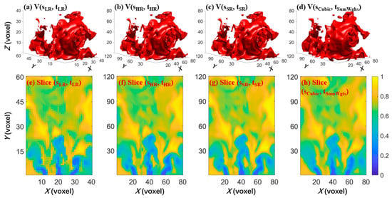
Figure 8.
Visual comparison of spatiotemporal SR network and cubic interpolation: (a–d) 3D structure topography and (e–h) 2D central slice.
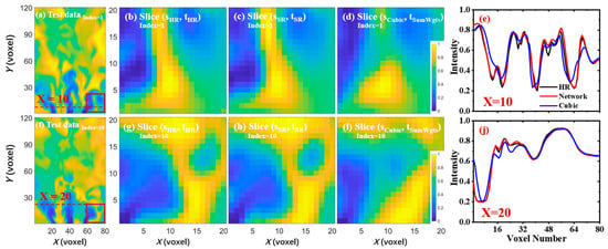
Figure 9.
Zoomed illustration of a local area and intensity variation with the inbetweening results of different methods. (e) One-dimensional comparison of the results at the X = 10 red dashed line. (j) One-dimensional comparison of the results at the X = 20 red dashed line.
Even so, it is still a little laborious to directly observe the superior Slice(, ) over Slice(, ). Hence, we amplified several local regions and performed intensity variation comparison to better illustrate the visual difference. Figure 9b–d are locally zoomed views of 2D slices, as marked with a red rectangle in the test data sample of Figure 9a. It can be seen obviously by an eye-ball check that there is almost no visual difference between the SR results and the original HR data, while the cubic interpolation results cannot accurately restore the characteristic distribution. To aid the visual examination of the SR effect in space and time, Figure 9e further illustrates the variation of the flame intensity along a horizontal line, as depicted by dashed red line in Figure 9a with X = 10. We can see that the intensity variation of the spatiotemporal SR model was in better agreement with the ground truth, while the cubic interpolation had a significant deviation. Moreover, Figure 9f–j supplement the local enlarged view and intensity variation of another flame at a different time instant. As before, the Slice(, ) still maintained an obvious advantage over Slice(, ) by recovering more detailed topographic features. The intensity signal of inbetweening displays more anastomotic agreement with HR data in Figure 9j. These above demonstrations illustrate how our model can effectively reconstruct the inbetweening volume with high resolution and accurate signal variation by using a deep learning network.
It is necessary to investigate the performance of noise immunity of our network, owing to the presence of various forms of noise when it comes to the SR of any practical 3D flame, such as calibration uncertainty, reconstruction error, and shot noise. Without updating the network parameters, the reconstruction performance with varying strengths of random noise was added to the original V(, ). The different magnitudes of noise were added to the test data according to Equation (5),
where amp represents the amplitude of random noise. The amplitudes were 1%, 3%, and 5% in turn. Figure 10 displays the noise immunity performance of the pre-trained network with amp = 1%, 3%, and 5%, as evaluated by the three metrics of the PSNR, ER, and SSIM. Such added noise caused the degradation of the SR quality. As can be seen from Figure 10, the metrics of PSNR, ER, and SSIM almost held unchanged with amp = 1%. When amp increased to 3% and 5%, the mean value of PSNR decreased by 3 dB and 5.4 dB, the mean value of ER rose by 0.9% and 1.8%, and the mean values of SSIM decreased by 0.024 and 0.056, respectively. Nevertheless, the variation in Figure 10 displays a satisfactory generalization performance for unforeseen noise. It is noted that the weight parameters of our model did not update specifically when using the extra added noise. Therefore, the consistently better performance proved that the proposed network was somehow immune to the random noise, and an even better reconstruction quality can be expected if the noisy input is used in training.

Figure 10.
Degradation of SR quality due to salt-and-pepper noise added. (a) variation of PSNR; (b) variation of ER; (c) variation of SSIM.
According to the quantitative evaluation of Figure 10 and the detailed visual comparisons of 3D, 2D, and 1D perspectives from Figure 8 and Figure 9, it is proven that we not only realized an excellent spatiotemporal reconstruction of the 3D flame structure but also conducted extensive evaluations to demonstrate the superiority of the model compared with other direct interpolation methods. Moreover, Figure 10 further illustrates the noise immunity of our proposed network on the spatiotemporal SR.
3.2. Spatiotemporal SR Based on Jet Flame
To explore the applicability of the proposed spatiotemporal SR reconstruction model to 3D turbulent flames, we further supplemented the verification of the model’s performance using jet flame data. The low spatiotemporal resolution data size here was 40 × 40 × 80, and the high spatiotemporal resolution data size was 80 × 80 × 160. Without making any changes to the network, the training process of the network was completed using an equal number of datasets and the same data preprocessing method as the swirling flame dataset, and the universality of the network was verified.
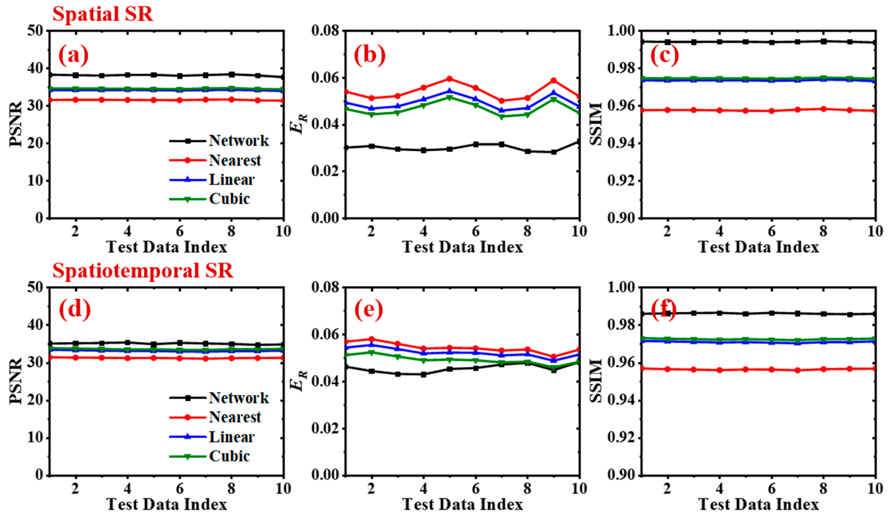
In Figure 11, Figure 12 and Figure 13, we further evaluate the applicability of the current spatiotemporal SR model by investigating the turbulent jet flame. We explored the same sequence of spatial SR first, followed by temporal SR, to show the universality of SR reconstruction of turbulent flame fields. The conventional interpolation techniques were also used for comparison. Here, we used the current model to rebuild the spatiotemporal HR data from the 3D jet flame LR data. Initially, Figure 11 quantitatively displays the reconstruction quality using global evaluation metrics, including spatial SR and ultimate spatiotemporal SR flame. As shown in Figure 11a–c, the results of the spatial SR process exhibited excellent reconstruction performance with the PSNR and SSIM mean values of 38.1 dB and 0.994, respectively, and the ER mean value of 2.9%. Such performance significantly exceeded any other interpolation methods, which are consistent as shown above in Figure 5 and can provide high-precision input for the temporal SR model. We then combined the spatial SR reconstruction with temporal inbetweening to obtain the spatiotemporal HR data V(, ), while the corresponding reconstruction results of interpolation methods were also obtained by the foregoing described procedures in the same way as swirling flame. As summarized in Figure 11d–f, cubic interpolation stayed ahead of the three methods, as was the case previously. The results of spatiotemporal SR remained superior to interpolation methods with the highest PSNR and SSIM mean values of 38.1 dB and 0.994, respectively, and the lowest ER mean value of 2.9%. Such results are consistent with the reconstruction of the swirling flame displayed in Figure 7.
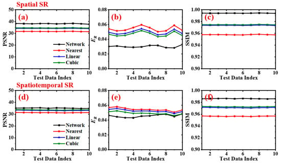
Figure 11.
The performance of the 3D spatiotemporal reconstruction model for jet flame: (a–c) the immediate results of spatial SR; (d–f) the ultimate results of spatiotemporal SR.
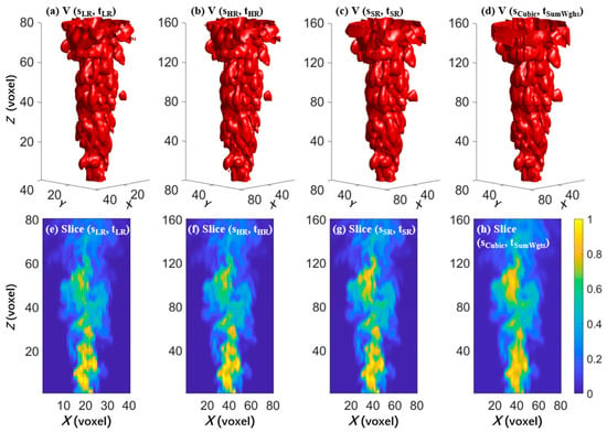
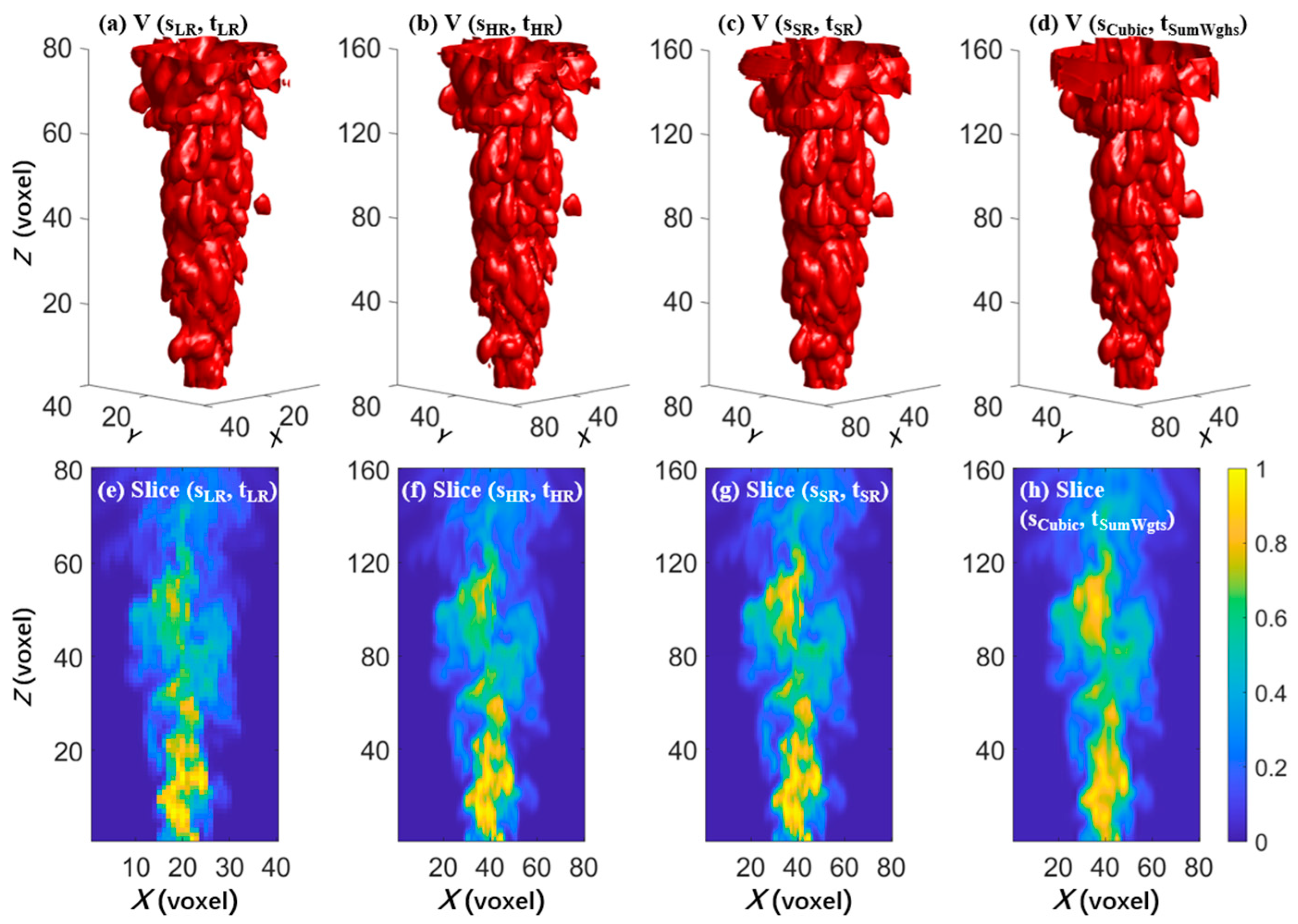
Figure 12.
Visual comparison of the spatiotemporal SR reconstruction of jet flame: (a–d) 3D structure; (e–h) 2D central slice.
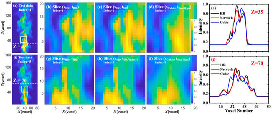
Figure 13.
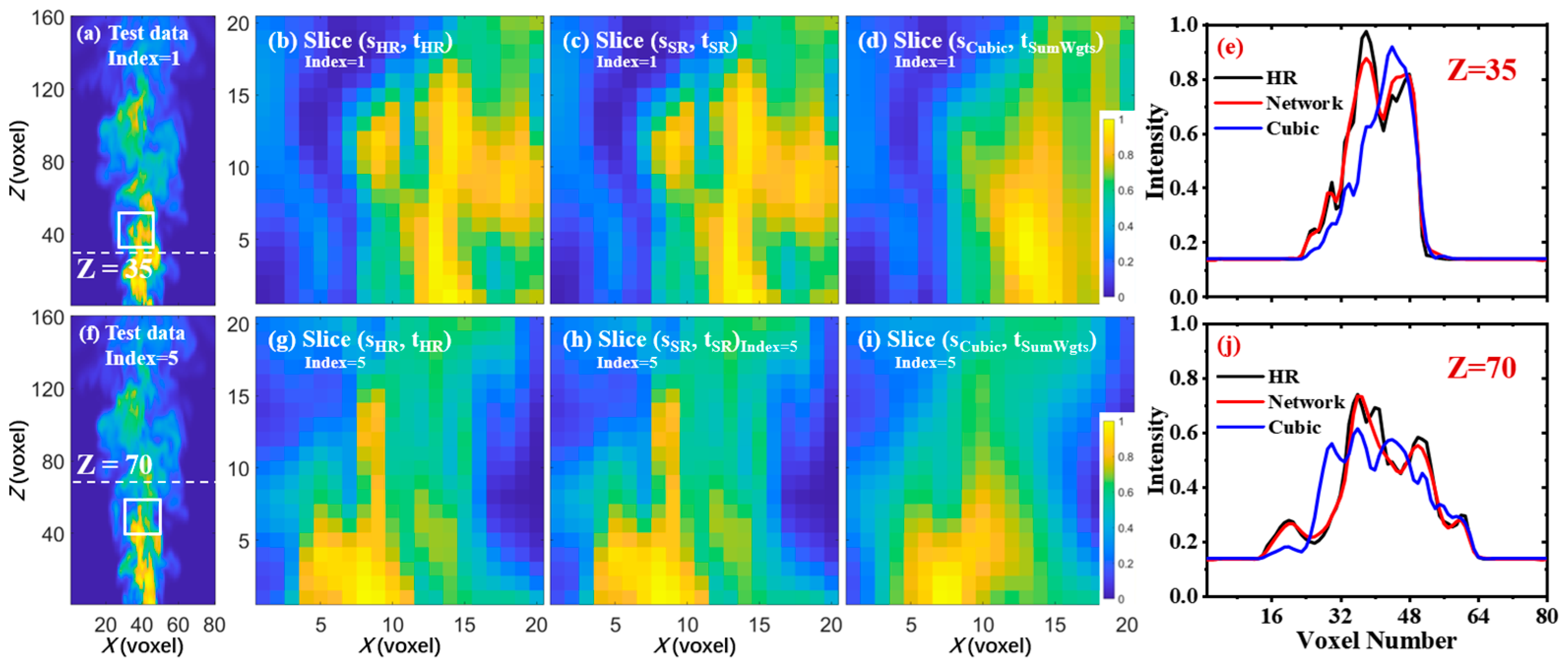
Local amplification and intensity variation comparison of the spatiotemporal SR results of jet flame. (e) One-dimensional comparison of the results at the Z = 35. (j) One-dimensional comparison of the results at the Z = 70.
Figure 12 displays the 3D structure rendering and 2D slice of the V(, ), V(, ), V(, ), and V(, ). It can be found that the V(, ) is visually closer to the V(, ) with recovering more detailed flow structures, while the V(, ) shows obvious distortion at the top of Figure 12d. Figure 12e–h extract 2D central slices along the Y coordinate from Figure 12a–d to easily distinguish the difference among the results of different methods. We find that the cubic interpolation over-smoothened the flowfield and cannot accurately reconstruct the small scales of the target flowfield very well. This implies that the cubic interpolation is unsuitable for highly turbulent flame reconstruction with many small-scale features. However, our presented approach can accurately reconstruct these small-scale structures that are not included in the input data. As shown in Figure 12g, Slice(, ) clearly shows a better reproduction to resolve such features, especially in the low-temperature region, which indicates the potential of the proposed model in capturing the dynamic characteristics of turbulent flow/combustion from coarse input data.
Figure 13 shows the 2D and 1D comparisons for a better evaluation. Figure 13b–d,g–i show zoomed views for 2D slices, as marked with red rectangles in Figure 13a,f, which denote two different time points. As in the previous demonstration of swirling flame, the cubic was still not able to recover the complete texture details. Conversely, the flow field was well recovered using the spatiotemporal SR model, as shown in Figure 13c,h. Figure 13e,j present comparisons of the 1D intensity variation in the reconstruction results along the horizontal lines, corresponding to the dashed red lines with Z = 35 and 70 in Figure 13a,f, respectively. It can be seen that the intensity variation of the model SR results is in good agreement with the HR data, while the cubic interpolation exhibits obvious deviations from ground truth. Again, this proves that our proposed algorithm not only effectively reconstructs the spatiotemporal HR field but also accurately recovers the original intensity distribution.
Figure 14 examines the noise immunity of the proposed spatiotemporal SR network on the turbulent jet flame. The generation of noisy input was also performed as in Equation (5) by using random noise. As can be seen from Figure 14, the three parameters, namely, PSNR, ER, and SSIM, exhibited similar variation with the increase in noise intensity as demonstrated in Figure 10, which means our model has fine generalization for possible random noise. It is worth emphasizing that the model has a certain degree of interference resistance to random noise of varying intensities without the need to retrain the parameters. This characteristic is crucial for practical applications, because in the real world, noise is inevitable in both experimental measurements and data acquisition. For instance, in the field of combustion diagnostics, flame imaging systems may be affected by various sources of noise, including uncertainties in equipment calibration, reconstruction errors, and photographic noise. The model proposed in this paper can maintain a high level of reconstruction quality in the presence of noise, indicating its potential application value in processing actual flame data. Specifically, the model’s noise resistance capability can reduce reliance on high-precision measurement equipment, lower costs, and enhance the ability to obtain reliable flame structure information in complex or noisy environments. Therefore, this study not only provides a new method for flame data processing in theory but also demonstrates its significant potential in solving real-world problems in practical applications.

Figure 14.
Validation of noise immunity for the pre-trained model by jet flame. (a) variation of PSNR; (b) variation of ER; (c) variation of SSIM.
4. Conclusions
In this study, a GAN architecture was used to construct a 3D spatiotemporal SR model. The spatial resolution and frequency of the flame sequence were both increased as a result of the model’s ability to forecast the intermediate HR frame that occurs between two successive coarse flow fields. Many inferences can be made from the work that has been provided. The PSNR and SSIM were higher than 6.42 dB and 0.038, respectively, and the ER was lower than 0.9% when compared to cubic interpolation, which is the best direct interpolation method. Moreover, the visual comparison and intensity distribution maintained great accuracy and congruence with the real world. The jet flame evaluation was used to confirm the universality of the suggested model. Furthermore, the pre-trained SR inbetweening model is capable of showing certain immunity to noise without retraining network parameters. Future work could focus on training the model on a more diverse range of datasets to be applied to other types of flames or turbulent structures, or conducting experimental validations to confirm the model’s effectiveness in real-world flame diagnostics. Additionally, enhancing the model’s interpretability and visualization will provide clearer insights into the model’s decision-making process. By addressing these areas, we are confident that the performance of our model can be further improved, broadening its applicability to a wider range of applications.
Author Contributions
Validation, C.Z.; writing—original draft, W.H.; writing—review and editing, W.X. All authors have read and agreed to the published version of the manuscript.
Funding
This research was funded by National Science and Technology Major Project (J2019-III-0022-0066) and the National Nature Science Foundation of China (no. 52006184).
Institutional Review Board Statement
Not applicable.
Informed Consent Statement
Not applicable.
Data Availability Statement
The data presented in this study are available on request from the corresponding author due to privacy concerns involving others.
Conflicts of Interest
The authors declare no conflicts of interest.
References
- Dreizler, A.; Böhm, B. Advanced laser diagnostics for an improved understanding of premixed flame-wall interactions. Proc. Combust. Inst. 2015, 35, 37–64. [Google Scholar] [CrossRef]
- Cai, W.; Li, X.; Li, F.; Ma, L. Numerical and experimental validation of a three-dimensional combustion diagnostic based on tomographic chemiluminescence. Opt. Express 2013, 21, 7050–7064. [Google Scholar] [CrossRef]
- Xu, W.; Carter, C.D.; Hammack, S.; Ma, L. Analysis of 3D combustion measurements using CH-based tomographic VLIF (volumetric laser induced fluorescence). Combust. Flame 2017, 182, 179–189. [Google Scholar] [CrossRef]
- Miller, V.A.; Troutman, V.A.; Hanson, R.K. Near-kHz 3D tracer-based LIF imaging of a co-flow jet using toluene. Meas. Sci. Technol. 2014, 25, 075403. [Google Scholar] [CrossRef]
- Cho, K.Y.; Satija, A.; Pourpoint, T.L.; Son, S.F.; Lucht, R.P. High-repetition-rate three-dimensional OH imaging using scanned planar laser-induced fluorescence system for multiphase combustion. Appl. Optics 2014, 53, 316–326. [Google Scholar] [CrossRef]
- Wellander, R.; Richter, M.; Aldén, M.J.E.I.F. Time-resolved (kHz) 3D imaging of OH PLIF in a flame. Exp. Fluids 2014, 55, 1764. [Google Scholar] [CrossRef]
- Wellander, R.; Richter, M.; Aldén, M. Time resolved, 3D imaging (4D) of two phase flow at a repetition rate of 1 kHz. Opt. Express 2011, 19, 21508–21514. [Google Scholar] [CrossRef]
- Liu, N.; Ma, L. Hybrid diagnostic for optimizing domain size and resolution of 3D measurements. Opt. Lett. 2018, 43, 3842–3845. [Google Scholar] [CrossRef] [PubMed]
- Xu, W.; Liu, N.; Ma, L. Super resolution PLIF demonstrated in turbulent jet flows seeded with I2. Opt. Laser Technol. 2018, 101, 216–222. [Google Scholar] [CrossRef]
- Grauer, S.J.; Unterberger, A.; Rittler, A.; Daun, K.J.; Kempf, A.M.; Mohri, K. Instantaneous 3D flame imaging by background-oriented schlieren tomography. Combust. Flame 2018, 196, 284–299. [Google Scholar] [CrossRef]
- Mohri, K.; Görs, S.; Schöler, J.; Rittler, A.; Dreier, T.; Schulz, C.; Kempf, A. Instantaneous 3D imaging of highly turbulent flames using computed tomography of chemiluminescence. Appl. Optics 2017, 56, 7385–7395. [Google Scholar] [CrossRef]
- Bao, Y.; Jia, J.; Polydorides, N. Real-time temperature field measurement based on acoustic tomography. Meas. Sci. Technol. 2017, 28, 074002. [Google Scholar] [CrossRef]
- Halls, B.R.; Hsu, P.S.; Roy, S.; Meyer, T.R.; Gord, J.R. Two-color volumetric laser-induced fluorescence for 3D OH and temperature fields in turbulent reacting flows. Opt. Lett. 2018, 43, 2961–2964. [Google Scholar] [CrossRef]
- Meyer, T.R.; Halls, B.R.; Jiang, N.; Slipchenko, M.N.; Roy, S.; Gord, J.R. High-speed, three-dimensional tomographic laser-induced incandescence imaging of soot volume fraction in turbulent flames. Opt. Express 2016, 24, 29547–29555. [Google Scholar] [CrossRef]
- Ma, L.; Wu, Y.; Lei, Q.; Xu, W.; Carter, C.D. 3D flame topography and curvature measurements at 5 kHz on a premixed turbulent Bunsen flame. Combust. Flame 2016, 166, 66–75. [Google Scholar] [CrossRef]
- Xu, W.; Luo, W.; Wang, Y.; You, Y. Data-driven three-dimensional super-resolution imaging of a turbulent jet flame using a generative adversarial network. Appl. Optics 2020, 59, 5729–5736. [Google Scholar] [CrossRef]
- Ling, C.; Chen, H.; Wu, Y. Development and validation of a reconstruction approach for three-dimensional confined-space to-mography problems. Appl. Optics 2020, 59, 10786–10800. [Google Scholar] [CrossRef]
- Ma, L.; Wickersham, A.J.; Xu, W.; Peltier, S.J.; Ombrello, T.M.; Carter, C.D. Multi-angular Flame Measurements and Analysis in a Supersonic Wind Tunnel Using Fiber-Based Endoscopes. J. Eng. Gas. Turbines Power 2016, 138, 021601. [Google Scholar] [CrossRef]
- Ma, L.; Lei, Q.; Wu, Y.; Xu, W.; Ombrello, T.M.; Carter, C.D. From ignition to stable combustion in a cavity flameholder studied via 3D tomographic chemiluminescence at 20 kHz. Combust. Flame 2016, 165, 1–10. [Google Scholar] [CrossRef]
- Dong, R.; Lei, Q.; Zhang, Q.; Fan, W. Dynamics of ignition kernel in a liquid-fueled gas turbine model combustor studied via time-resolved 3D measurements. Combust. Flame 2021, 232, 111566. [Google Scholar] [CrossRef]
- Halls, B.R.; Hsu, P.S.; Jiang, N.; Legge, E.S.; Felver, J.J.; Slipchenko, M.N.; Roy, S.; Meyer, T.R.; Gord, J.R. kHz-rate four-dimensional fluorescence tomography using an ultraviolet-tunable narrowband burst-mode optical parametric oscillator. Optica 2017, 4, 897–902. [Google Scholar] [CrossRef]
- Halls, B.R.; Gord, J.R.; Meyer, T.R.; Thul, D.J.; Slipchenko, M.; Roy, S. 20-kHz-rate three-dimensional tomographic imaging of the concentration field in a turbulent jet. Proc. Combust. Inst. 2017, 36, 4611–4618. [Google Scholar] [CrossRef]
- Veeraraghavan, S.M.; Kaliyaperumal, G.; Dillikannan, D.; De Poures, M.V. Influence of Hydrogen induction on performance and emission characteristics of an agricultural diesel engine fuelled with cultured Scenedesmus obliquus from industrial waste. Process Saf. Environ. Prot. 2024, 187, 1576–1585. [Google Scholar] [CrossRef]
- De Poures, M.V.; Dillikannan, D.; Kaliyaperumal, G.; Thanikodi, S.; Ağbulut, Ü.; Hoang, A.T.; Mahmoud, Z.; Shaik, S.; Saleel, C.A.; Afzal, A. Collective influence and optimization of 1-hexanol, fuel injection timing, and EGR to control toxic emissions from a light-duty agricultural diesel engine fueled with diesel/waste cooking oil methyl ester blends. Process Saf. Environ. Prot. 2023, 172, 738–752. [Google Scholar] [CrossRef]
- Sathish, T.; Ağbulut, Ü.; Ubaidullah, M.; Saravanan, R.; Giri, J.; Shaikh, S.F. Waste to fuel: A detailed combustion, performance, and emission characteristics of a CI engine fuelled with sustainable fish waste management augmentation with alcohols and nanoparticles. Energy 2024, 299, 131412. [Google Scholar] [CrossRef]
- McManus, T.A.; Papageorge, M.J.; Fuest, F.; Sutton, J.A. Spatio-temporal characteristics of temperature fluctuations in turbulent non-premixed jet flames. Proc. Combust. Inst. 2015, 35, 1191–1198. [Google Scholar] [CrossRef]
- Patton, R.A.; Gabet, K.N.; Jiang, N.; Lempert, W.R.; Sutton, J.A. Multi-kHz temperature imaging in turbulent non-premixed flames using planar Rayleigh scattering. App. Phys. B 2012, 108, 377–392. [Google Scholar] [CrossRef]
- Roy, S.; Hsu, P.S.; Jiang, N.; Slipchenko, M.N.; Gord, J.R. 100-kHz-rate gas-phase thermometry using 100-ps pulses from a burst-mode laser. Opt. Lett. 2015, 40, 5125–5128. [Google Scholar] [CrossRef]
- Cheng, X.; Ren, F.; Gao, Z.; Wang, L.; Zhu, L.; Huang, Z. Predicting 3D distribution of soot particle from luminosity of turbulent flame based on conditional-generative adversarial networks. Combust. Flame 2023, 247, 112489. [Google Scholar] [CrossRef]
- Zhang, W.; Dong, X.; Liu, C.; Nathan, G.J.; Dally, B.B.; Rowhani, A.; Sun, Z. Generating planar distributions of soot particles from luminosity images in turbulent flames using deep learning. Appl. Phys. B 2021, 127, 18. [Google Scholar] [CrossRef]
- Carreon, A.; Barwey, S.; Raman, V. A generative adversarial network (GAN) approach to creating synthetic flame images from experimental data. Energy AI 2023, 13, 100238. [Google Scholar] [CrossRef]
- Fukami, K.; Fukagata, K.; Taira, K. Machine-learning-based spatio-temporal super resolution reconstruction of turbulent flows. J. Fluid Mech. 2021, 909, A9. [Google Scholar] [CrossRef]
- Zhang, W.; Dong, X.; Sun, Z.; Zhou, B.; Wang, Z.; Richter, M. 100 kHz CH2O imaging realized by lower speed planar laser-induced fluorescence and deep learning. Opt. Express 2021, 29, 30857–30877. [Google Scholar] [CrossRef]
- Guo, H.; Zhang, W.; Nie, X.; Dong, X.; Sun, Z.; Zhou, B.; Wang, Z.; Richter, M. High-speed planar imaging of OH radicals in turbulent flames assisted by deep learning. App. Phys. B 2022, 128, 52. [Google Scholar] [CrossRef]
- Fukami, K.; Fukagata, K.; Taira, K. Super-resolution reconstruction of turbulent flows with machine learning. J. Fluid Mech. 2019, 870, 106–120. [Google Scholar] [CrossRef]
- Kim, H.; Kim, J.; Won, S.; Lee, C. Unsupervised deep learning for super-resolution reconstruction of turbulence. J. Fluid Mech. 2021, 910, A29. [Google Scholar] [CrossRef]
- Kim, J.; Lee, C. Prediction of turbulent heat transfer using convolutional neural networks. J. Fluid Mech. 2020, 882, 18. [Google Scholar] [CrossRef]
- Sidey, J.A.M.; Giusti, A.; Benie, P.; Mastorakos, E. The Swirl Flames Data Repository. Available online: http://swirl-flame.eng.cam.ac.uk (accessed on 20 May 2023).
- Tyliszczak, A.; Cavaliere, D.E.; Mastorakos, E. LES/CMC of Blow-off in a Liquid Fueled Swirl Burner. Flow Turb. Comb. 2014, 92, 237–267. [Google Scholar] [CrossRef]
- Cai, M.; Jin, H.; Lin, B.; Xu, W.; You, Y. Numerical Demonstration of Unsupervised-Learning-Based Noise Reduction in Two-Dimensional Rayleigh Imaging. Energies 2022, 15, 5747. [Google Scholar] [CrossRef]
- Xu, W.; Luo, W.; Chen, S.; You, Y. Numerical demonstration of 3D reduced order tomographic flame diagnostics without angle calibration. Optik 2020, 220, 165198. [Google Scholar] [CrossRef]
- Barlow, R.S.; Frank, J.H. Effects of turbulence on species mass fractions in methane/air jet flames. Symp. Combust. 1998, 27, 1087–1095. [Google Scholar] [CrossRef]
- Jones, W.P.; Prasad, V.N. Large Eddy Simulation of the Sandia Flame Series (D–F) using the Eulerian stochastic field method. Combust. Flame 2010, 157, 1621–1636. [Google Scholar] [CrossRef]
- Nair, V.; Hinton, G.E. Rectified linear units improve restricted boltzmann machines. In Proceedings of the 27th International Conference on International Conference on Machine Learning, Omnipress, Haifa, Israel, 21–24 June 2010; pp. 807–814. [Google Scholar]
- He, K.; Zhang, X.; Ren, S.; Sun, J. Deep Residual Learning for Image Recognition; IEEE: Piscataway, NJ, USA, 2016. [Google Scholar]
- Jakhetiya, V.; Kumar, A.; Tiwari, A.K. A survey on image interpolation methods. In Proceedings of the Second International Conference on Digital Image Processing, Singapore, 26–28 February 2010; SPIE—The International Society for Optical Engineering: Bellingham, WA, USA, 2010. [Google Scholar]
- Lehmann, T.M.; Gonner, C. Survey: Interpolation methods in medical image processing. IEEE Trans. Med. Imaging 1999, 18, 1049–1075. [Google Scholar] [CrossRef]
- Keys, R.G. Cubic convolution interpolation for digital image processing. IEEE Trans Acoust. Speech Signal Process. 1981, 29, 1153–1160. [Google Scholar] [CrossRef]
- Yang, C.-Y.; Ma, C.; Yang, M.-H. Single-Image Super-Resolution: A Benchmark. In Proceedings of the Computer Vision—ECCV 2014, Zurich, Switzerland, 6–12 September 2014; Fleet, D., Pajdla, T., Schiele, B., Tuytelaars, T., Eds.; Springer International Publishing: Cham, Switzerland, 2014; pp. 372–386. [Google Scholar]
- Wang, Z.; Bovik, A.C.; Sheikh, H.R.; Simoncelli, E.P. Image quality assessment: From error visibility to structural similarity. IEEE Trans. Image Process 2004, 13, 600–612. [Google Scholar] [CrossRef]
Disclaimer/Publisher’s Note: The statements, opinions and data contained in all publications are solely those of the individual author(s) and contributor(s) and not of MDPI and/or the editor(s). MDPI and/or the editor(s) disclaim responsibility for any injury to people or property resulting from any ideas, methods, instructions or products referred to in the content. |
© 2024 by the authors. Licensee MDPI, Basel, Switzerland. This article is an open access article distributed under the terms and conditions of the Creative Commons Attribution (CC BY) license (https://creativecommons.org/licenses/by/4.0/).

