1. Introduction
The United States is in an era of increasing wildfire activity, with recent decadal trends and future projections all pointing towards larger and more frequent fires burning under more extreme weather conditions [
1,
2,
3,
4,
5]. This, combined with the expansion of communities and infrastructure into fire-prone wildlands, has increased the demand for wildfire suppression [
6,
7,
8]. As a result, more firefighters are exposed to workplace hazards while managing increasingly complex wildfires [
9,
10,
11]. Wildland firefighters complete arduous work, often in remote settings with multiple hazards capable of causing serious or even life-threatening injuries (fire, smoke, steep and uneven terrain, extreme weather, motorized equipment, falling or rolling objects, etc.) [
12,
13,
14,
15].
Firefighters have instituted a variety of protocols aimed at minimizing the risk to their wellbeing on the fireline, such as the 10 Standard Fire Orders, the 18 Watch Out Situations, and LCES (Lookouts, Communications, Escape routes, Safety zones), that largely depend on firefighters in the field recognizing and avoiding or mitigating hazards [
16,
17,
18]. More recently, spatial models of firefighting opportunity, difficulty, and safety have been developed [
19,
20,
21,
22,
23], to help incident managers design safe and effective fire response strategies through risk-based decision frameworks promoted by the Wildland Fire Decision Support System (WFDSS) and the USDA Forest Service, Strategic Analytics Branch, Risk Management Assistance (RMA) dashboard [
24,
25,
26].
Spatial information on potential evacuation times or other firefighter safety concerns can complement field-level risk management at the strategic planning phase, by helping incident managers avoid committing firefighters to high-risk tactics. Long evacuation times increase the risk to firefighters, and prompt access to medical care is key to reducing injury consequences. Fires in more remote areas (distant from hospitals, farther along minor road networks, and/or deeper into off-road settings) have longer medical evacuation times. In the absence of air support for evacuations, long ground travel times may prevent injured firefighters from receiving proper care within a medically critical time frame.
There is an extensive body of work surrounding the spatial analysis of health care access (e.g., [
27,
28,
29,
30,
31,
32]). Particularly noteworthy among these efforts is a recent global mapping of travel times to health care facilities [
30]. Although these maps could conceivably be used in the context of wildland fire management, their relatively coarse (1 km) resolution may limit their applicability at the scale of operational fire decision-making. Another valuable contribution in this research arena is AccessMod 5, a software program supported by the World Health Organization that can map the travel time to medical facilities [
32]. However, it only takes the slope of the terrain into account for off-road travel. Beyond slope, wildland firefighters are faced with wide-ranging landscape impediments in the rugged, unimproved areas where they often work [
33,
34].
The wildland firefighter estimated ground evacuation time (GET) model is a spatially explicit quantification of ground evacuation time to the nearest relevant medical facility, which is designed to help evaluate potential firefighter safety risks and inform safe and effective fire response strategies [
23]. The GET model was originally developed in 2013 (this previous version will henceforth be referred to as GET v1) to inform strategic planning with a better awareness of potential evacuation challenges and the risks that long evacuation times pose to firefighters [
23]. According to a recent survey, GET v1 was one of the most frequently used datasets for strategic planning from the decision support layers promoted by the Risk Management Assistance Program [
35]. Despite its wide use, GET v1 has not been updated or modified since its initial creation to account for changing landscape conditions (e.g., hospital locations, road networks, and land cover) and advancements in our understanding of how landscape characteristics affect pedestrian movement [
33,
36,
37]. The primary objective of this paper is to introduce a new version of GET (henceforth referred to as GET v2) and describe its motivation, methods, intended uses, and limitations. In the interest of promoting an informed continuity of product use, we compare GET v2’s methodology and results to those of GET v1, to make users aware of key differences and their implications for use. We also compare the travel times predicted by GET v2 to actual firefighter evacuation times compiled from incident reports.
2. Materials and Methods
2.1. Methods Summary
There are three main components to GET. The first is the medical facilities, or hospitals, of interest. The geographic distribution of appropriate medical facilities that provide the right kinds of care for injured firefighters plays a major role in dictating evacuation times. The second component is the road transportation network. The road network dictates from how far, at what speeds, and from what directions vehicles can access capable medical facilities. The third and final component of GET is off-road travel. Wildland firefighters often work in remote, off-road locations. Thus, the distance and landscape conditions between the crew and the vehicle-accessible road network also affect the total medical evacuation time. The combination of these three components provides a suitable approximation of the travel portion of a medical evacuation timeline.
Taking these three components into account, the workflow for generating GET v2 proceeded as follows (
Figure 1). First, an appropriate set of hospitals was selected from a dataset of medical facilities, to ensure that a minimum level of relevant care could be provided. For example, a pediatric or rehabilitation care facility may not be suitable for treating injured firefighters. From each of the resulting hospitals, the outward-looking travel time was calculated. The travel time was assumed to be reciprocal for this analysis, such that the time it takes to travel between a hospital and a particular location on the landscape should be the same irrespective of travel direction. The outward-looking travel time was based first and foremost on on-road travel rates, which were derived from road speed categories, based on speed limits, surface types, etc. From each point along a road, representing a potential place where a vehicle may be parked, the off-road travel time was added. The off-road travel time considered a wide range of landscape conditions, including slope, vegetation type, fuel structure, the presence of water features, and the presence of minor roads or trails. The total travel time for each hospital was estimated on a per-pixel basis at a 30 m spatial resolution, out to a total travel time of six hours. These travel time raster datasets were then combined, by taking the minimum travel time for each pixel to create a new CONUS-wide representation of minimum on- and off-road total travel time to the nearest relevant hospital (GET v2).
GET v2 is based on the concept of least-cost path modeling. Least-cost path modeling is a well-established, widely used geospatial modeling technique that identifies the path of least resistance between two or more locations on a landscape, given a set of spatially explicit constraints [
38]. It relies on some measure of “cost” that represents the impedance (or friction, resistance, etc.) between locations on a landscape. In the absence of cost, the least-cost path between two points (e.g., a hospital and a firefighter) would be a straight line. In a realistic landscape, the presence of roads and various landscape features that we account for in our analysis either promote or hinder efficient movement. Thus, the aforementioned outward-looking travel time calculation from each hospital relied on the creation of a “cost surface”—a raster dataset where each pixel represents how long it would take to traverse that pixel, taking into account the many factors that affect movement. From each hospital, and to each nearby pixel, the least-cost path was generated up to a point where the maximum travel time of interest (six hours) was accumulated in all directions. All data processing was performed using Esri ArcGIS Pro version 3.2.1.
Throughout the development of GET v2, we sought and received input from a stakeholder group comprising federal geospatial and wildland fire professionals. The group played a particularly important role in the methodological decision-making, where expert opinion was required. These decision points included the identification of a relevant set of medical facilities, and the assignment of travel costs for landscape factors that influence off-road pedestrian travel.
2.2. Component #1: Hospitals
In this section, we describe the process we used to select an appropriate set of medical facilities for use in GET. Medical facilities are the foundation of GET, representing the endpoints of the travel time analysis. GET v1 utilized a hospital dataset from the National Geospatial-Intelligence Agency’s Homeland Security Infrastructure Program (HSIP) filtered to identify “definitive care” facilities (i.e., excluding urgent care clinics) within CONUS [
23]. For GET v2, we used the best-available hospital dataset with similar attributes and nation-wide coverage from the Homeland Infrastructure Foundation-Level Data (HIFLD). The data, produced for the U.S. Department of Homeland Security’s Geospatial Management Office, were last updated in September 2023. Our group of subject matter experts favored a similarly inclusive representation of hospitals as GET v1, meant to approximate facilities capable of stabilizing patients with serious injuries, rather than a more restricted set of higher capability hospitals that tend to be concentrated in major cities. The hospital selection criteria for GET v2 were based on two attributes from the HIFLD hospitals dataset:
STATUS: we selected hospitals labeled as being “OPEN” (as opposed to “CLOSED”);
TYPE: we selected hospitals labeled as being either “GENERAL ACUTE CARE” or “CRITICAL ACCESS”. This excluded many medical facility types like “PYSCHIATRIC”, “REHABILITATION”, “LONG TERM CARE”, etc. that are unlikely to accept patients with acute care needs.
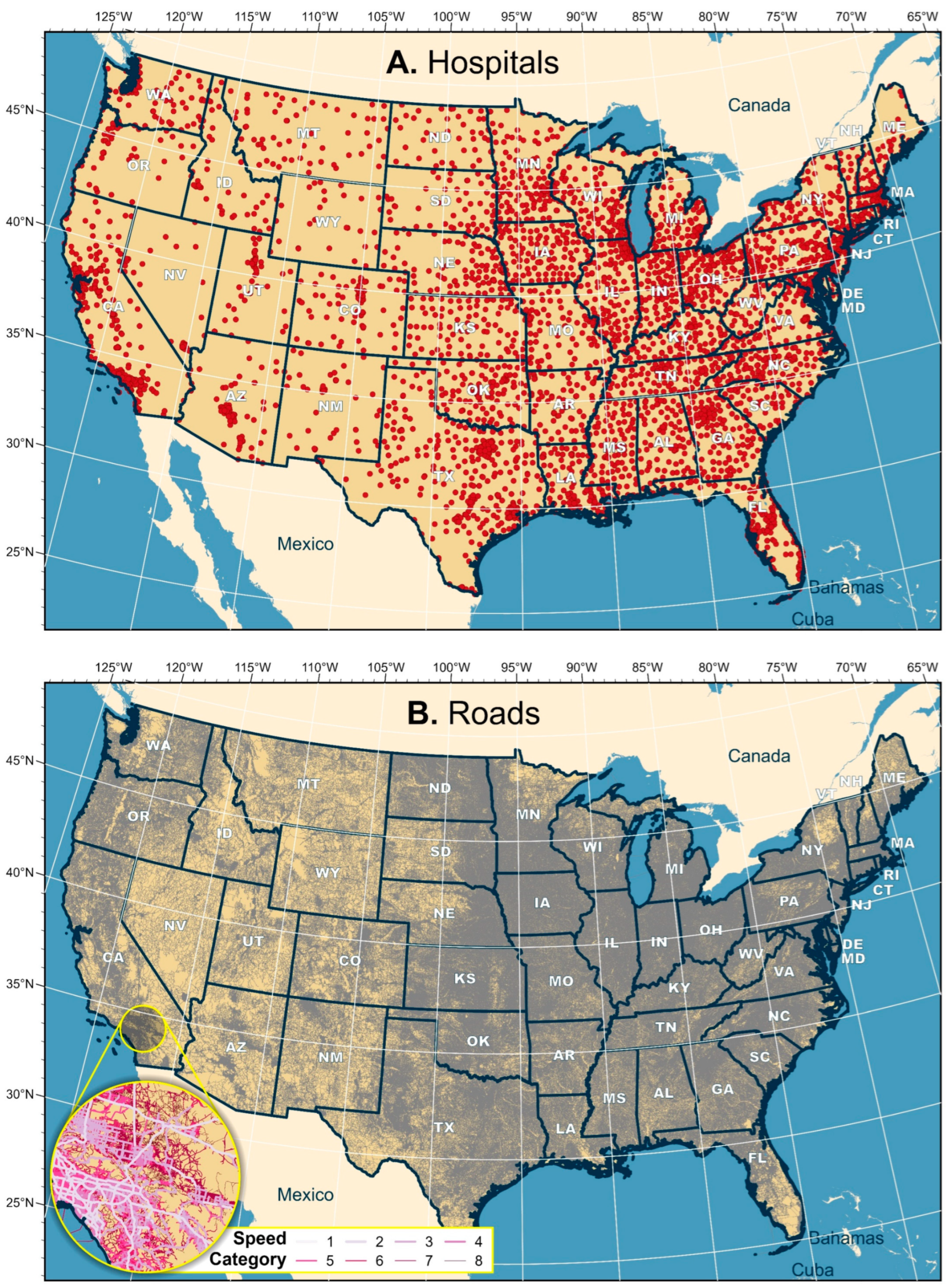
After filtering for these two criteria, we ended up with 5136 hospitals in CONUS that served as the basis of GET v2 (
Figure 2A).
2.3. Component #2: On-Road Travel
The second component of GET v2 is on-road travel time. In this section, we describe the process we used to acquire a CONUS-wide road dataset and attribute appropriate travel costs. GET v1 relied on a road network dataset from NAVTEQ, version 2010.2, generated in September 2010 [
23]. For this analysis, we used the HERE roads network published in 2020 from HIFLD, which is a contemporary version of the earlier NAVTEQ data. The most relevant attribute in HERE for estimating on-road travel time is the “Speed Category” field (SpeedCat), which “classifies the general speed trend of a road based on posted or implied speed limit” (
Table 1,
Figure 2B). Consistent with GET v1, we translated the speed category into representative speed values that fall within the category speed ranges (
Table 1). To convert these speeds (where high values mean faster travel, in miles per hour) to costs (where high values mean slower travel, in seconds per meter), we applied the conversion from Equation (1) below:
where
is seconds per meter (cost),
is a conversion factor for seconds per hour, equal to 3600 s,
is the selected speed value, in miles per hour, and
is a conversion factor for meters per mile, equal to 1609.34 m.
Although HERE data were initially in a vector polyline format, we opted to convert the HERE roads to raster for consistency with the off-road travel time analysis. Each 30 m pixel containing road was assigned the appropriate cost value from
Table 1.
2.4. Component #3: Off-Road Travel
The third and final component of GET v2 is the off-road travel time. This section features five subsections (
Section 2.4.1,
Section 2.4.2,
Section 2.4.3,
Section 2.4.4 and
Section 2.4.5), wherein we describe how the off-road travel time was calculated based on landscape characteristics that affect pedestrian movement. GET v1 treated off-road travel in a fairly simple manner, with only a few categorical land cover and slope classes dictating speeds (
Table 2). GET v2 both adds nuance to the land cover and slope-based travel rate estimates and a suite of new impediments firefighters often face in wildland settings.
There is a growing body of scientific literature exploring how landscape conditions affect pedestrian travel rates or energy exertion (e.g., [
33,
34,
36,
37,
39,
40,
41]). However, the vast array of landscape conditions that wildland firefighters may face well exceeds the confines of what has been studied in a robust, quantitative manner (i.e., through field experiments or crowdsourcing user GPS tracks). Accordingly, where available, we leveraged scientifically robust information for the assessment of off-road travel time. For example, the relationship between slope and travel rates has been well studied, so we were able to use a robust slope–travel rate equation to serve as the basis for assigning slope-based costs [
36]. Where we were unable to leverage existing travel rate functions, we relied on expert knowledge accrued from the many years of experience traversing complex landscapes possessed by the authors, as well as the broader subject matter expert group.
The off-road travel time calculation is summarized in
Figure 1. Briefly, it began with the relationship between slope and travel rates. If a pixel’s slope was steeper than 45 degrees, or if it was mapped as being a major water feature, it was treated as an impassible barrier. If a pixel was mapped as being a trail or a minor road not mapped in the HERE roads data, no additional cost beyond that associated with slope was applied (as indicated by the “1×” in
Figure 1). If the land cover was grass or non-burnable, no additional cost was applied. If it was mapped as tree-dominated, then a 4× cost multiplier was applied. For instance, if slope dictated that a pixel had a travel rate of 1 m·s
−1 (or, inversely, a time cost of 1 s·m
−1), then the resulting cost of traversing that pixel in a forest would be 4 s·m
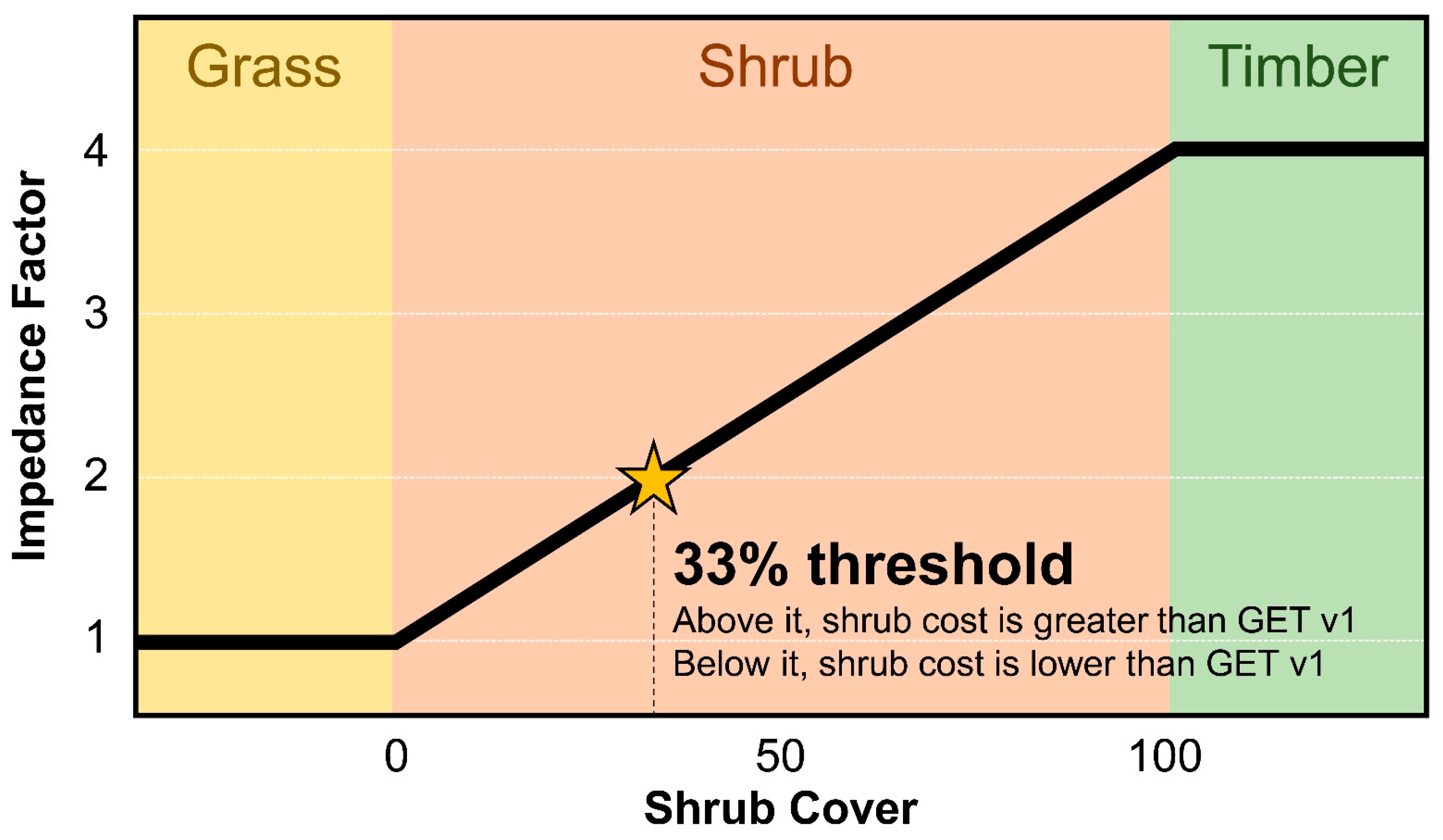
−1. If the land cover was mapped as shrub, then we applied a shrub cover-based cost multiplier ranging from 1× (0% shrub cover) to 4× (100% shrub cover). To account for the additional challenge of traversing forests with abundant coarse woody debris (i.e., logging slash, wind blowdowns, post-fire debris, etc.), we applied an additional either 2× or 5× cost multiplier, depending on the fuel type. Lastly, if a pixel traversed a perennial stream too small to be mapped by the land cover data, a 5× cost multiplier was further applied. Note that these costs accrue in a multiplicative fashion. For example, traveling through a tree-dominated environment (4× cost) that is also mapped as a timber litter slash/debris fuel type (2× cost), the resulting cost would be 8 times the slope-based cost. More detail is provided on data sources and cost calculations in each of the following sections.
2.4.1. Slope Cost
Below, we describe the basis of how we calculated travel rates as a function of terrain slope. Generally, the relationship between slope and travel rates is such that steeper slopes, both uphill and downhill, tend to slow one down while traveling on foot. The specific quantitative nature of that relationship has been explored in many studies [
33,
36,
37,
39,
42,
43,
44,
45,
46,
47,
48,
49,
50,
51]. Most resulting slope–travel time functions are slightly asymmetrical or anisotropic, meaning that the same slope uphill and downhill will produce minor differences in travel rates. This makes intuitive sense—traveling on steep slopes is challenging in both directions but is less physically demanding downhill than uphill. However, the quantitative complexity of applying an anisotropic (directional) cost accumulation on a broad spatial scale acts as a limiting factor. Accordingly, for GET v2, we constructed a new symmetrical/isotropic travel rate function. To do this, we reexamined data from Campbell et al. (2022) [
36] with a travel rate function form that omitted the terms that made the function asymmetrical, which can be seen in Equation (2):
where
is travel rate (in m·s
−1),
is slope (in degrees), and
,
, and
are model coefficients determined from a non-linear least squares regression analysis of Campbell et al. (2022)’s [
36] crowdsourced GPS-tracked hiking data.
was found to be equal to 22.4056,
was equal to 77.6196, and
was equal to 0.0464. This reduces Equation (2) to Equation (3):
To convert Equation (3) (rate, in m·s
−1), into a travel cost (in s·m
−1), we calculated its reciprocal (Equation (4)):
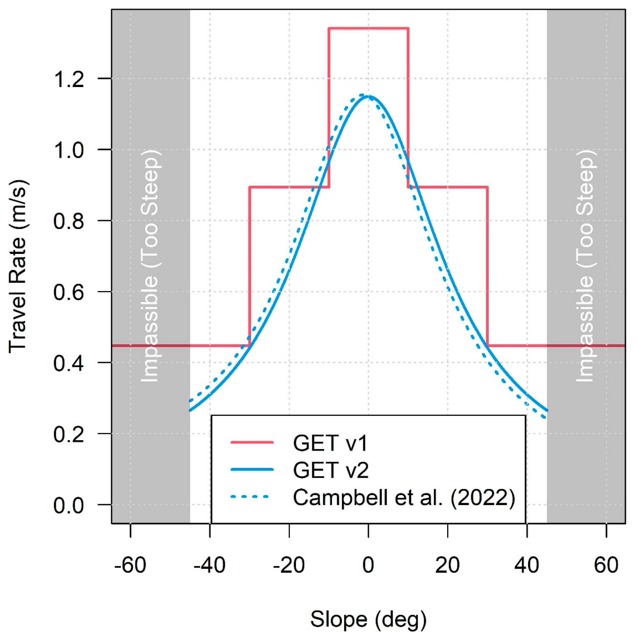
In a departure from GET v1, we opted to consider slopes greater than 45 degrees impassible barriers, given both the physical challenge and safety risk associated with traversing such extreme slopes, especially while assisting or carrying an injured firefighter.
Figure 3 compares GET v1 and GET v2 slope–travel rate functions, assuming no additional travel costs. GET v2 yields a more conservative estimate of maximum walking speeds and produces a more realistic set of values that vary continuously with slope. The symmetrical function used in GET v2 is very similar to the original, asymmetrical function from Campbell et al. (2022) [
36], yielding an average difference (RMSE) of 0.038 m·s
−1 between the two (
Figure 3). To derive a CONUS-wide, spatially explicit representation of slope cost, we used the slope data from LANDFIRE, released in 2020, with a pixel resolution of 30 m.
2.4.2. Land Cover Cost
In this section, we detail how different land covers, including the proportional canopy cover of shrub-dominated areas, affected travel rates in GET v2. Land cover characteristics also influence pedestrian travel. For example, traversing dense, tall vegetation is slower than traversing sparse or no vegetation. The specific quantitative relationship between vegetation structure and travel rates has been explored only sparingly in the scientific literature [
33,
34,
37,
41]. In the absence of a more robust understanding of the complex effects that different land cover types have on walking speed, we opted to base GET v2’s land cover component on GET v1, with some important modifications. The land cover cost was based on a combination of the 2020 LANDFIRE Existing Vegetation Type (EVT) and Existing Vegetation Cover (EVC) datasets.
In GET v1, land cover was treated as an impediment using a 5-class system (
Table 2 and
Table 3). Our first modification from GET v1 was to treat grass and non-burnable as being functionally equivalent with respect to travel rates. Both possessed a 1× cost multiplier, meaning their travel rate was solely based on the slope of the underlying terrain without any additional cost. Secondly, whereas GET v1 enabled travel (albeit very slow travel) in water, to err on the side of safety, we have opted to treat water features large enough to be mapped as water in the EVT data (i.e., covering the majority of a 900 m
2 LANDFIRE pixel) as impassible barriers. Thirdly, we treat all tree-dominated areas as having a 4× cost multiplier, meaning one travels 4× slower through a forested area than a grass/non-burnable area on equivalent slopes. Lastly, we added a new cover-based impedance factor for shrub-dominated areas, described next.
We know from experience and limited scientific evidence that vegetation density within the height range of the human body has a direct impeding effect on travel rates [
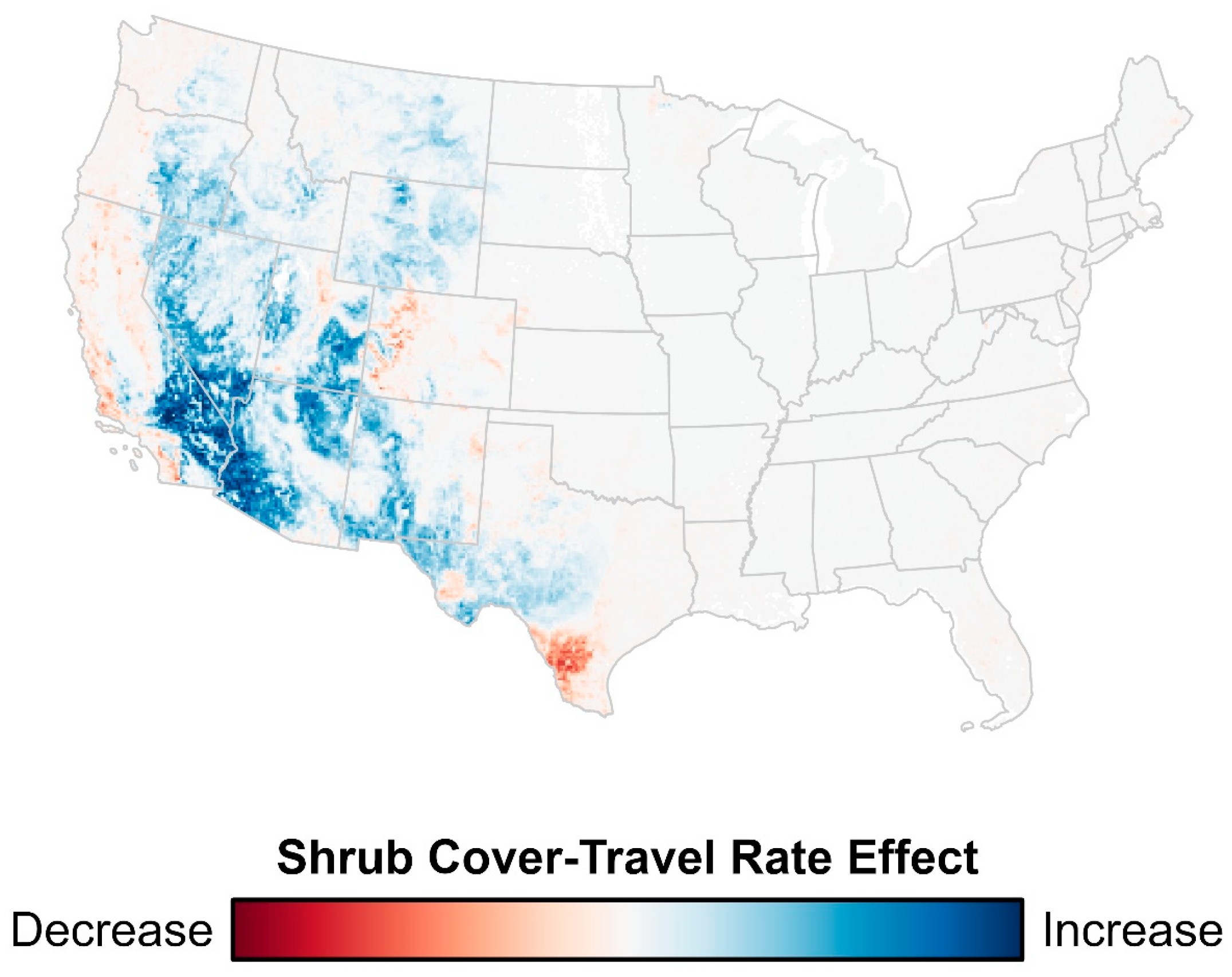
33]. If we had a CONUS-wide representation of low-lying vegetation density, we could leverage this information in GET v2. No such dataset exists at present, limiting our ability to directly map density-based impedance. However, by definition, areas mapped as being shrub-dominated in the EVT data feature vegetation similar in height to humans. Furthermore, LANDFIRE EVC offers life form-specific canopy cover estimates. The impedance one would experience traveling through very sparse (e.g., 10% cover) shrubs would be very similar to traveling through grassland. On the opposite extreme, traveling through very dense (e.g., 90% cover) shrubs would be comparable to (and in some cases potentially even slower than) traveling through a forest. Thus, we can leverage the shrub cover data to map impedance on a continuous basis, ranging from a 1× impedance factor on the low cover end to a 4× impedance factor on the high cover end (
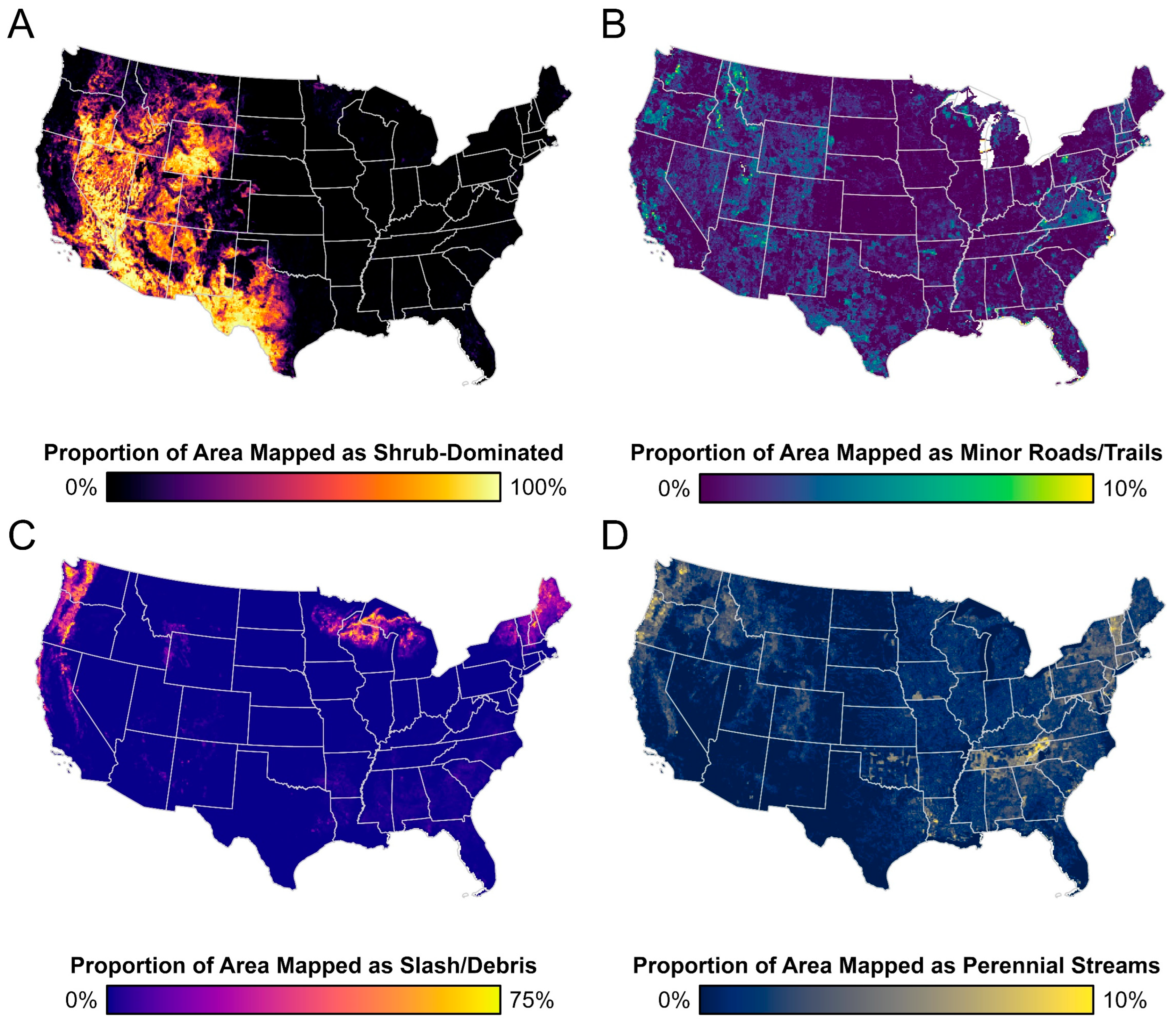
Figure 4). We know, in practice, that some tree-dominated environments are easier and faster to traverse than some dense shrub-dominated environments, but we could not use tree cover in the same way that we used shrub cover to obtain a more nuanced indicator of low-lying vegetation density. High tree canopy cover does not necessarily correlate to (and may in fact be inversely related to) low-lying vegetation density. Thus, we maintained that all tree-dominated environments have a 4× cost multiplier. In comparison to GET v1, the equivalent shrub cost in GET v2 would occur at approximately 33% cover, such that shrubs with a higher cover than that represent an increase in apparent travel cost and shrubs with a lower cover represent a decrease in cost over the previous version.
2.4.3. Minor Road/Trail Cost
Here, we explain the inclusion of minor roads and trails as low-cost landscape features in GET v2. The HERE roads data are very extensive and capture the vast majority of the drivable roads in the US (
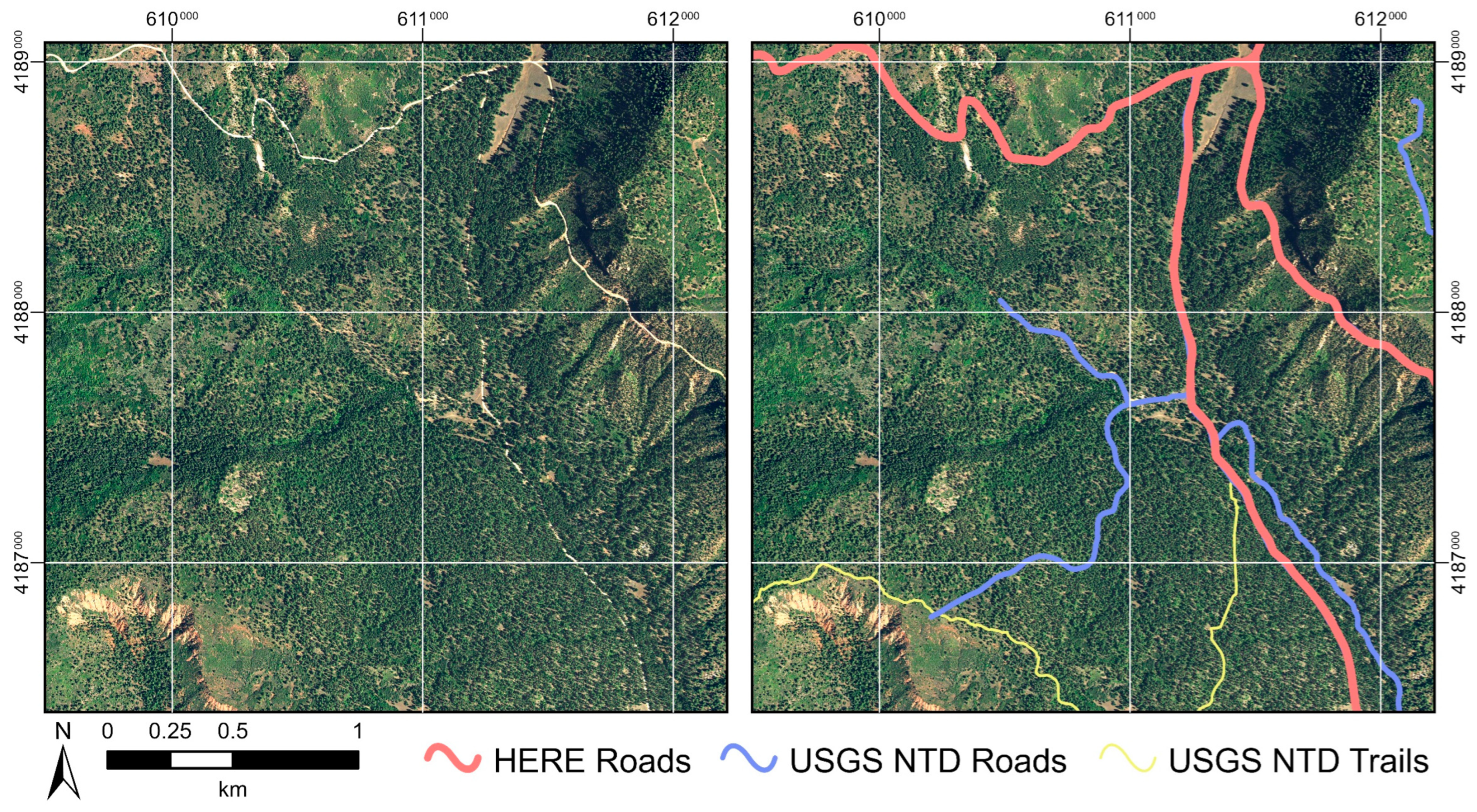
Figure 2B). However, in the remote areas where firefighters often work, there are many miles of minor roads and trails that are not captured in the HERE data. On one hand, this exclusion may be useful for erring on the side of caution; minor roads may not be reliably accessible to vehicles due to lack of improvement or maintenance. Accordingly, our on-road travel time component was limited to roads mapped by HERE. However, even if a vehicle cannot reliably access a minor road or trail, it may still represent a useful feature to walk on. In
Figure 5, for example, the left pane features an aerial image with two prominent forest roads that are mapped by HERE in the right pane. However, there are also several features not mapped by HERE, but included in the USGS National Transportation Dataset (NTD) that may still represent a useful set of pedestrian pathways for firefighters. Given the option to walk through a forest or on an even poorly maintained minor forest road or trail, firefighters would likely opt to walk along the road/trail. To incorporate the minor roads/trails not mapped in HERE as a representation of the best case for off-road travel, all pixels that intersected roads and trails mapped in the USGS NTD were assigned the same land cover cost multiplier as grass/non-burnable (1×), meaning no additional cost greater than that of slope alone was associated with those areas.
2.4.4. Slash/Debris Cost
Below, we describe our process for incorporating woody debris as a new cost into GET v2. Our subject matter experts determined that it would be a useful to consider the cost associated with traveling through settings with abundant coarse woody debris. Post-fire landscapes where trees have fallen, forests that have experienced major insect, disease, or windthrow events, post-logging areas with a high concentration of slash, and even just forests with high loads of coarse woody debris are all very challenging and slow to walk through. To emphasize the additional travel cost in these settings, we used the 2020 LANDFIRE 40 Scott and Burgan Fire Behavior Fuel Models (also known as the “FBFM40”) [
52]. We identified seven FBFM40 classes associated with high coarse woody debris loads (
Table 4). The three timber litter (TL) fuel-type models were attributed with a 2× cost multiplier, whereas the four slash–blowdown (SB) fuel-type models were given a 4× multiplier. Note that these costs are multiplied by all the other previously described costs (i.e., slope and land cover cost). All told, these slash and debris classes represent a relatively small proportion of the US, but there are several regions with a high cover of the selected fuel models that see meaningful impacts on GET v2 (
Figure 6).
2.4.5. Stream Cost
The LANDFIRE EVT maps large water bodies (i.e., oceans, lakes, major rivers), but omits most small water features (i.e., streams). As mentioned earlier, we have opted to make these larger water features impassible in GET v2, given the risk and difficulty of crossing them. Small streams are considerably easier to traverse than large water bodies. However, to ignore them entirely fails to capture the decrease in walking speeds through water and over loose, slippery, and/or uneven bed material. For GET v2, we have opted to include smaller perennial (i.e., containing a persistent flow of water) streams as additional impediments. To that end, we used the USGS National Hydrography Dataset Plus High Resolution (NHDPlus HR) streams data. All perennial streams were attributed with an additional multiplicative cost multiplier of 5× and rasterized at a 30 m resolution.
2.5. Modeling GET v2 and Comparing It to GET v1
In this subsection, we detail our process for generating GET v2 from its various inputs and making comparisons to GET v1. A CONUS-wide, 30 m resolution, rasterized representation of travel cost was generated by combining on- and off-road travel times, following the logic seen in
Figure 1. Each pixel represented the cost, in s·m
−1, it would take to traverse the landscape conditions that pixel overlapped. This was then used to calculate travel times from each of the 5136 hospitals on a per-pixel basis, up to six total hours in travel time. This was accomplished using the Distance Accumulation function in ArcGIS, which iteratively accumulates cost from a given source (hospital) in all directions radiating outward until a maximum accumulated cost (six hours) is reached. Six hours was chosen to match the highest evacuation time class threshold in GET v1 (0–1 h; 1–2 h, 2–4 h, 4–6 h, >6 h). This yielded 5136 travel time raster datasets. The per-pixel combined minimum travel time across all 5136 rasters was calculated using the Cell Statistics function in ArcGIS. The resulting map was a CONUS-wide representation of the time it would take, in seconds, to reach the nearest hospital. This was then reclassified into the hour-based time intervals previously defined for GET v1.
To highlight areas where new data and methods are likely to drive differences in GET v2, we created maps of several relevant variables at a 10 km resolution. These included the following: (1) the proportion of 30 m LANDFIRE EVT pixels mapped as being shrub-dominated; (2) the proportion of 30 m pixels mapped as major roads; (3) the proportion of 30 m pixels mapped as a minor roads/trails pixel area within 10 km aggregated pixels; (4) the difference between (2) and (3), to highlight the areas where minor roads/trails are likely to affect GET v2 most significantly; (5) the proportion of 30 m LANDFIRE FBFM40 pixels mapped as being any of the seven fuel models from
Table 4 within 10 km aggregated pixels; and (6) the proportion of 30 m pixels that intersected NHD HR Plus perennial streams within 10 km aggregated pixels.
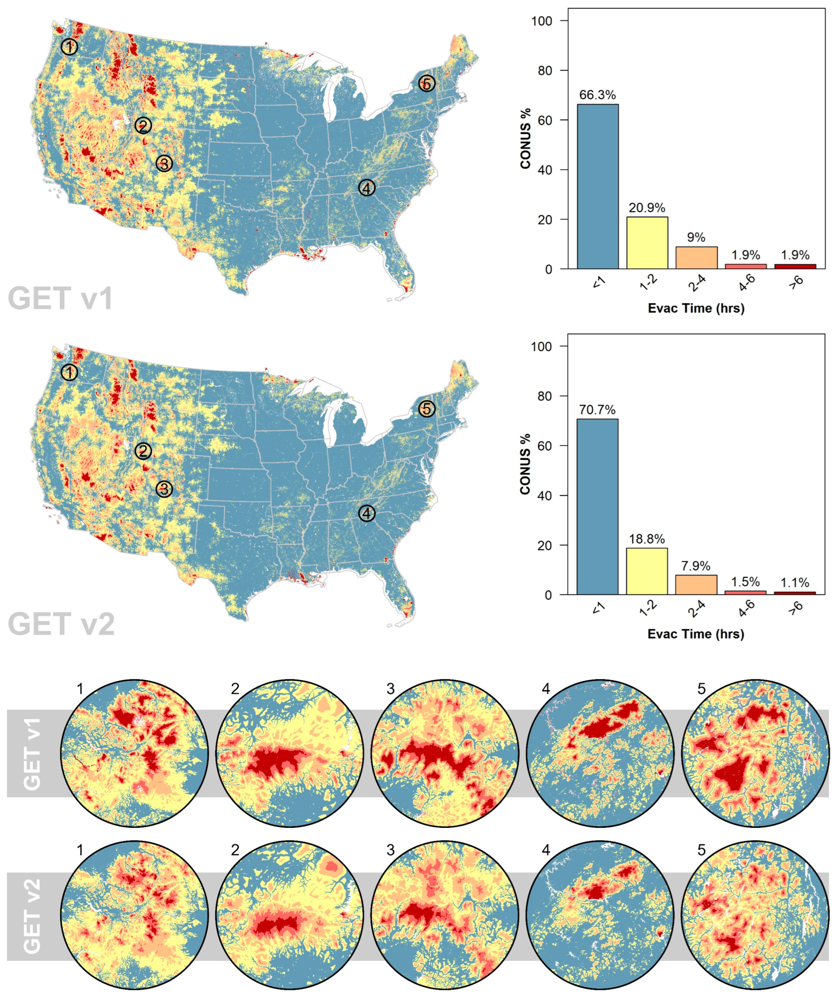
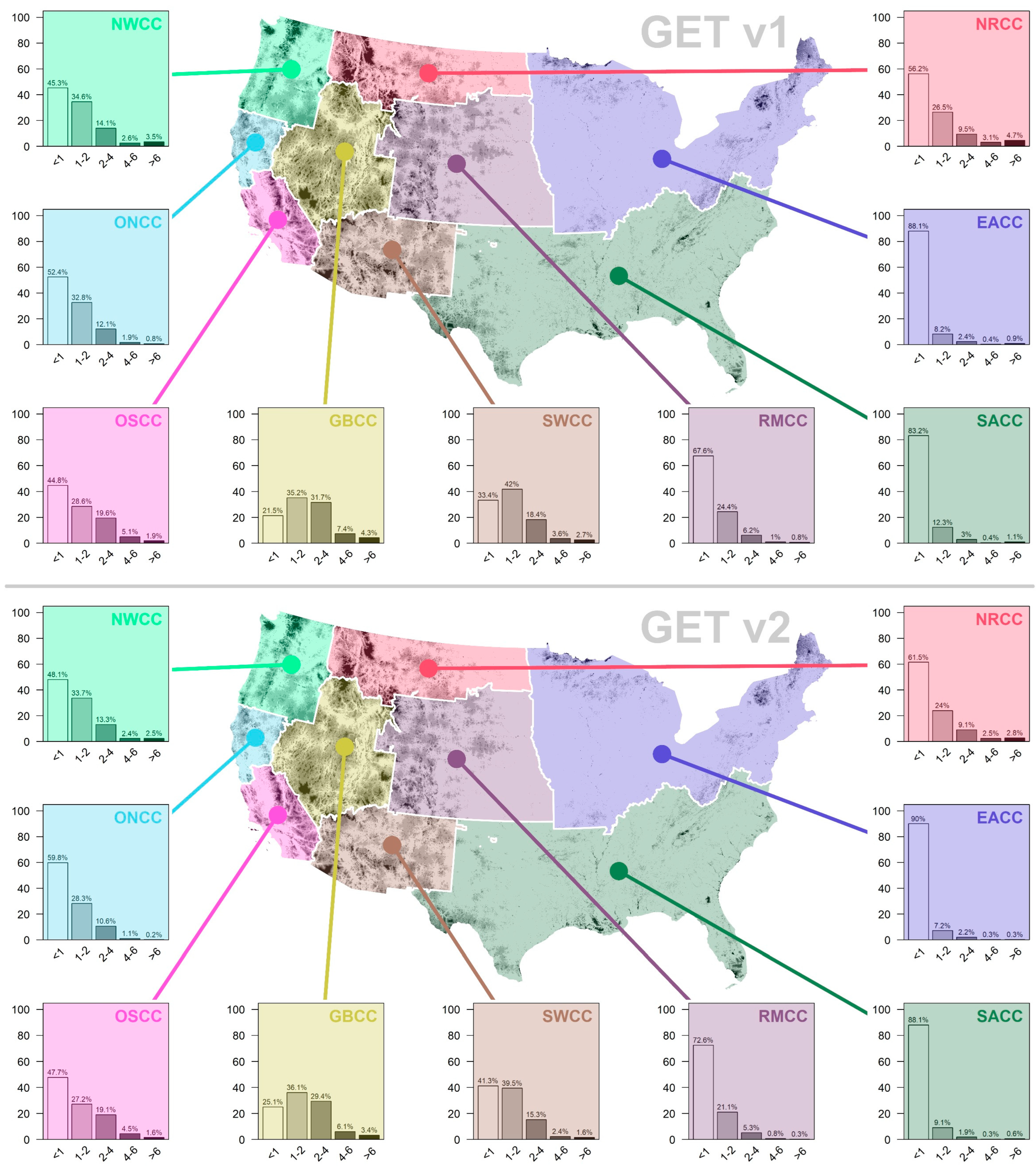
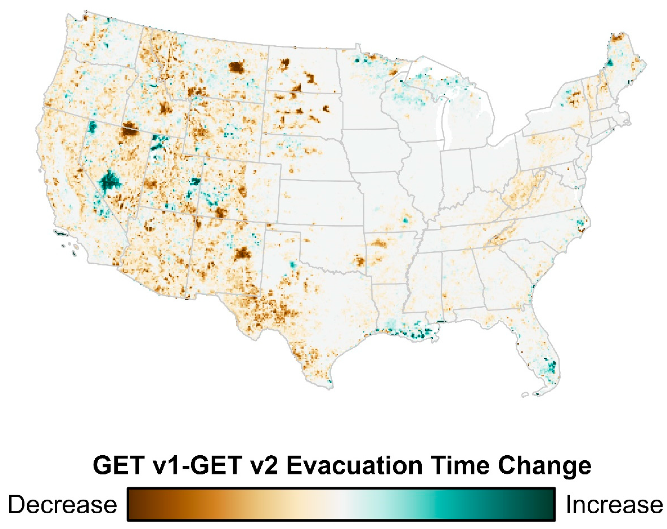
We compared the final GET v1 and GET v2 products in a few ways. The first comparison was generating time class histograms that tallied the proportion of 30 m pixels mapped at two scales: (1) within CONUS as a whole; and (2) broken down by Geographic Areas (GAs) used for wildland fire resource coordination. This provided a spatial and tabular summary of the overall national and regional differences between GET v1 and GET v2. The second comparison was a per-pixel time class comparison, yielding a matrix with proportions of mapped classes within CONUS for each overlapping cell in GET v1 and GET v2. This provided us with a detailed cross-tabulation of the relative class abundances and the per-pixel changes between product versions. The third and final comparison was a per-pixel image difference, where values were reclassified as an increased evacuation time (e.g., going from 0–1 h in GET v1 to 1–2 h in GET v1) (+1), unchanged (0), or decreased evacuation time (−1). These 30 m change pixels were aggregated up to 10 km using a mean function to represent regional patterns in increased or decreased evacuation time estimates.
2.6. Comparing GET v2 to Incident Report Data
The ideal dataset to evaluate GET v2 performance would include numerous wildland fire medical evacuation records, with precise spatial data and incident timelines stratified across a variety of injury types, crew configurations, and environments. In the absence of such data, we leveraged wildland fire accident, injury, and fatality reports from the Wildland Fire Histomap, a web portal representing recent and historical safety incidents in map form [
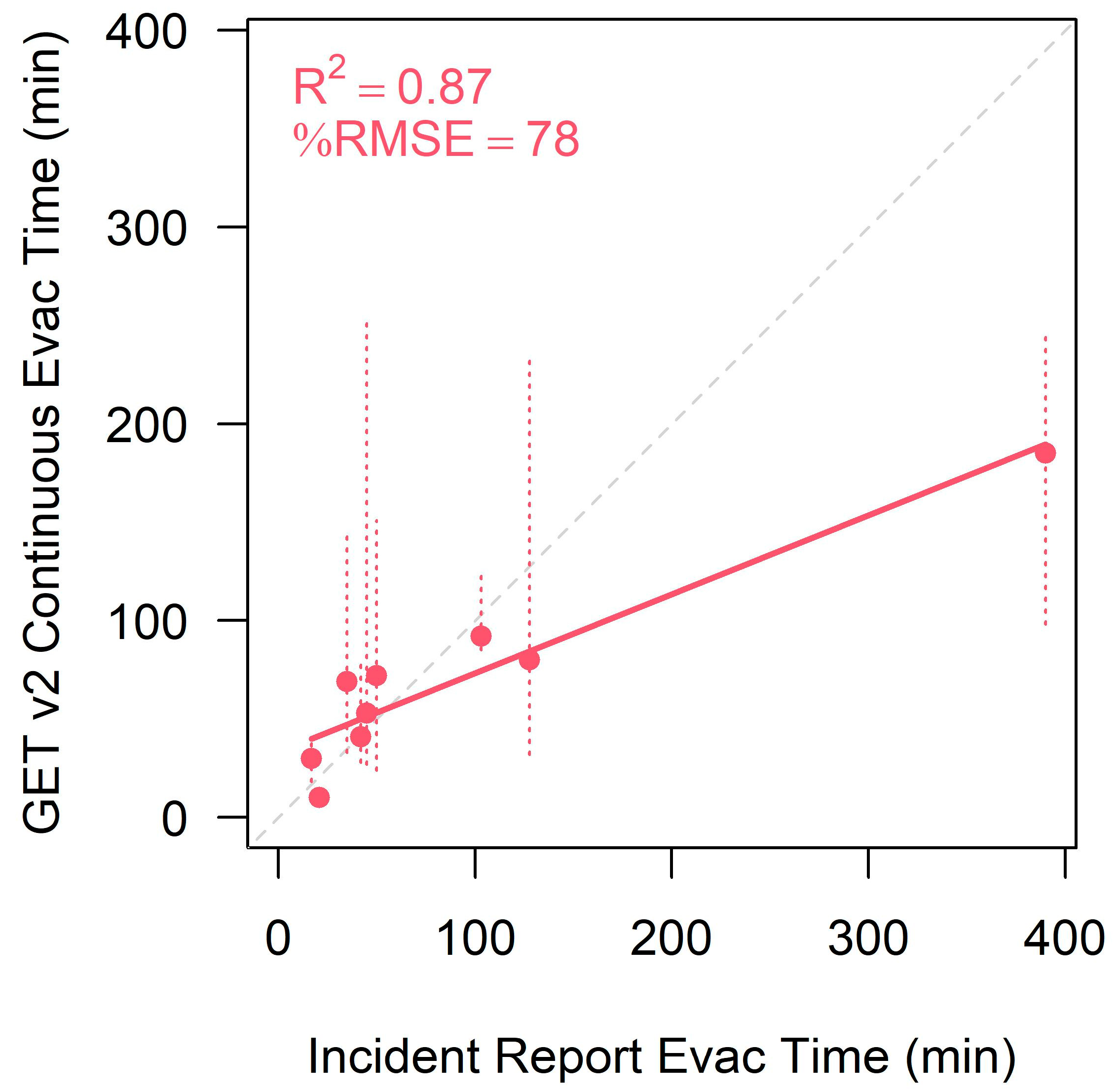
53], to evaluate GET v2’s alignment with evacuation times in real incidents. The wildland fire management community has a long history of documenting and learning from safety incidents, but reporting practices vary widely. We identified a subset of spatially explicit incident data that is most appropriate for comparison to GET v2 by leveraging attributes in the Histomap database and reviewing the associated incident reports. First, for temporal relevance, we only selected incidents that occurred since 2000. Second, we only included incidents where the sole method of evacuation was ground-based (i.e., not assisted by aviation) and the destination was a hospital. Third, we required that the evacuation time be described in the report. This yielded nine incidents. For each, we extracted an estimate of the travel time between the injury site and hospital from the incident reports.
The incident reports contained varying levels of detail on evacuation start (i.e., injury) locations for associating the incident with the GET v2 results. At best, incident reports included a map with a point location from which evacuation start coordinates could be approximated. At worst, no specific positional information was provided, other than the associated wildfire or prescribed fire name. For each incident, we generated a polygon that captured the uncertainty of evacuation start positional information. For high-confidence locations (n = 2), where incident reports contained a map with a point, the point was approximately digitized and buffered by 100 m to account for the digitizing uncertainty. For low-confidence locations (n = 4), where no positional information was provided, the perimeter of the fire or treatment was used. If they were wildfires (n = 2), a 1 km buffer was added to the fire perimeter to account for the possibility that incidents occurred during indirect attack. There were also three moderate-confidence incidents, where some additional spatial context was provided (e.g., road/trail names). In these cases, an appropriate buffer size was applied to the relevant landscape features according to the information provided. Within these nine polygons, we extracted the GET v2 evacuation time estimates in minutes. This approach assumes that the most accessible hospital was used, which matches the intended use of GET v2, and was necessary as most reports did not include the hospital name or location. The GET v2 estimates are also based on current landscape conditions (hospitals, roads, vegetation, etc.), which may differ from the landscape conditions at the time of our nine evaluation fires.
The reported evacuation times were compared to the range and median evacuation time values from GET v2 using a scatterplot and linear regression. The evaluation results should be interpreted cautiously, given the small sample size and uncertainty associated with extracting spatial information and timelines from unstandardized reports.
4. Discussion
Irrespective of the version, GET is meant to be used at broad spatial scales to help understand potential medical evacuation challenges and to encourage discussion of how to manage the associated risks to wildland firefighter safety. It is not meant to replace incident-level medical planning or to inform evacuation routing decisions. Those activities must be coordinated at the incident level, informed by local geographic and incident-specific knowledge and a careful consideration of real-time information that GET cannot account for. Accordingly, GET is represented in broad time classes to encourage users to focus on general patterns at landscape to regional scales.
GET occupies an important and unique niche within the existing body of spatial medical accessibility research. It shares some characteristics with efforts such as the global health care access maps from Weiss et al. [
30] and the software platform AccessMod 5 [
32], in that they all consider medical facilities, transportation networks, and landscape conditions in a least-cost path-driven spatial modeling context. However, GET is better suited for wildland fire management for several reasons, including its comparably high spatial resolution (30 m), the use of an improved slope–travel rate function, the use of current vegetation and fuels data, and the focus on incorporating more nuanced off-road landscape travel costs likely to be encountered by wildland firefighters.
There are several limitations to this product that warrant discussion. First and foremost, the input datasets upon which GET v2 is based (hospitals, roads, fuel, topography, etc.) possess inherent spatial and thematic uncertainty. That uncertainty propagates through the entire analytical workflow, making final evacuation time estimates likewise uncertain. Our evaluation of GET v2 with a limited sample of incident reports shows that the estimated evacuation times roughly align with field observations, but a more robust dataset is needed to quantify uncertainty across a wider range of environments. Developing such a dataset is a priority to inform future methods improvements. As increasing numbers of firefighters become equipped with global positioning systems receivers, a robust, data-driven evacuation validation procedure could be possible.
Second, to the maximum extent possible, we attempted to accurately represent the relative impedance factors associated with traversing both on- and off-road environments in a robust and broadly applicable manner. Although our slope–travel rate relationship was based on a scientifically robust study of pedestrian travel rates [
36], there simply are not enough studies that examine experimental or crowdsourced data representing the effects that landscape conditions have on walking speed. Absent them, we were left to make approximations based on the foundation laid by GET v1 and the authors’ and subject matter expert group’s personal experiences. More studies are needed in this critical area of research. Such work would have great benefits, not only for GET and within the fire management context, but to any discipline in which pedestrian–environment interactions are of focal interest.
Third, there are several factors that GET could not account for. For one, this product assumes that every pixel in CONUS is theoretically accessible, unless defined as a slope- or water-driven barrier. Given the focus on emergency response, we did not consider that land ownership or management type would influence travel, but there are situations in which fences, gates, or uncooperative landowners could slow or divert an evacuation. On-road travel rates are also based on a static speed category, which does not account for temporally dynamic phenomena such as traffic, stoplights, etc. Although it would require an immense computational capacity, incorporating more dynamic elements into GET could be feasible in the future to tailor estimates to current conditions or to estimate uncertainty in GET from dynamic factors.
Fourth, GET v2 only accounts for the travel portion of an evacuation and assumes that off-road travel will be taking place on foot at a typical walking pace. GET does not account for the time needed for patient assessment, care, packaging, or transfer to a vehicle, given the wide range of possible injury types and severities and the limited data available to estimate these evacuation components. In reality, an injured firefighter may have to be carried in a litter because they cannot walk. Doing so would slow travel rates, which GET does not account for. However, there are also situations where off-road vehicles could be used on minor roads, trails, or smooth terrain with short vegetation to recover an injured firefighter, which would act to significantly reduce the travel time. Thus, by assuming a typical walking speed, we feel we have balanced the wide range of evacuation conditions that could emerge.
Fifth, GET is based entirely on a least-cost path analysis to calculate the travel time from (and to) hospitals. By their very nature, the accumulated, per-pixel travel times that result from this type of analysis represent the minimum time it would take to reach each pixel, assuming the singular path of least resistance was taken. In reality, firefighters would likely take suboptimal paths when traveling from the injury site to the nearest vehicular access. So, even if the travel rate estimates were accurate on a per-pixel basis, the actual evacuation route will likely take longer than using the minimum time path. However, some byproducts of GET could conceivably be used for evacuation route mapping, thus improving the likelihood that optimal or nearly-optimal paths are taken during evacuation.
Given the importance of major roads in evacuation timing, and the emphasis on comparisons between GET v1 and GET v2 in this paper, a spatial comparison between the 2010 NAVTEQ roads data that drove GET v1 and the 2020 HERE roads data that drove GET v2 would have added value to our study. Unfortunately, the former dataset is not publicly available. Accordingly, such a comparison was not possible.
To fill gaps in the empirical research, we relied on expert opinion to drive what we intended to be a conservative representation of pedestrian travel times, erring on the side of caution for safety-focused fire response planning. For example, experience and intuition tells us that crossing a stream adds time to an evacuation, as does traversing dense woody debris—both factors previously omitted from GET v1. Thus, including them in GET v2, even if the specific multiplicative cost factors have not been independently validated, adds a useful degree of caution for risk assessment and mitigation planning. Expert opinion plays an important role in wide-ranging environmental modeling applications, particularly when empirical evidence is absent [
54]. It is widely used in the development of comparable wildland fire spatial decision support datasets, such as GET v1 and the Suppression Difficulty Index [
22,
23].
Improved data collection on future medical evacuations is a high priority to inform GET model improvements. Many of the incidents we considered for model evaluation could have made good case studies with better spatial and temporal reporting. Future report contributors should include spatial coordinates of the incident location, the name and town of the destination hospital, and well-attributed logs of evacuation activities and times. If possible, a GPS track could be collected to record the evacuation route and precisely document the timeline. Alternatively, some of the off-road travel factors accounted for in GET could be better refined with field experiments or non-evacuation observations of firefighter movement through complex terrain. As mentioned in the land cover methods section, our ability to apply the latest mobility research is sometimes limited by the availability of the appropriate spatial data (especially vegetation structure) needed to make predictions at regional or national scales.
Despite these limitations, GET provides a valuable a priori spatial awareness of potential risks, to help avoid exposing firefighters to hazards in areas with long evacuation times. GET communicates general trends in landscape accessibility that managers should take into consideration when planning fire responses, along with information on other firefighter safety concerns, management objectives, and the probability of suppression success, to determine if actions are warranted. There are no recommended maximum ground evacuation times for firefighters to engage a fire, but long evacuation times are a watch out situation that warrants careful consideration before committing resources. Engaging a fire in remote areas may be contingent on the ability to mitigate long evacuation times through, for example, helicopter availability and safe flying conditions or reopening abandoned roads to facilitate extraction via off-road vehicles. GET does not provide answers, but it is a tool to encourage an awareness of evacuation challenges and critical thinking as to how to minimize firefighter safety concerns at the strategic planning level.
While GET v2 shares many similarities with GET v1, there are some meaningful differences at regional and landscape scales that should be considered when applying the data for strategic planning. Regions with much higher evacuation times in GET v2 (
Figure 11) have either lost hospitals, decommissioned roads, or are impacted by one of the new off-road travel factors. Mitigation measures not typically considered in the past may be warranted for future incidents in these regions to counteract the decreased hospital accessibility. Incident-level medical planning is still important in regions with reduced evacuation times, but improved hospital accessibility may lower risks to firefighters and possibly reduce the reliance on aerial transport for medevacs. Landscape-level differences in GET and the consequences for incident-level response strategies depend strongly on how the new factors in the model (
Section 3.1;
Figure 6 and
Figure 7) interact to change local spatial patterns in travel costs and hospital accessibility. Portions of landscapes with low shrub cover or a high density of minor roads and trails will be perceived as less challenging for evacuations, while areas with high shrub cover, high woody debris loads, or an abundance of perennial streams will appear more difficult for evacuations. The most dramatic changes at landscape scale come from treating steep slopes and large waterbodies as barriers. Users should more easily recognize landscape features likely to divert and lengthen an evacuation route like a major river or cliff band.
Although we have described a product that is generated at the CONUS scale, wildland firefighter safety is an important concern well beyond the confines of our study area. By providing a detailed accounting of the datasets used to generate GET and explaining our analytical approach for estimating travel times, we hope that this work can serve as a foundation upon which similar products could be generated in other fire-prone regions of the world.

