Satellite Image Cloud Automatic Annotator with Uncertainty Estimation

Abstract

In satellite imagery, clouds obstruct the ground information, directly impacting various downstream applications. Thus, cloud annotation/cloud detection serves as the initial preprocessing step in remote sensing image analysis. Recently, deep learning methods have significantly improved in the field of cloud detection, but training these methods necessitates abundant annotated data, which requires experts with professional domain knowledge. Moreover, the influx of remote sensing data from new satellites has further led to an increase in the cost of cloud annotation. To address the dependence on labeled datasets and professional domain knowledge, this paper proposes an automatic cloud annotation method for satellite remote sensing images, CloudAUE. Unlike traditional approaches, CloudAUE does not rely on labeled training datasets and can be operated by users without domain expertise. To handle the irregular shapes of clouds, CloudAUE firstly employs a convex hull algorithm for selecting cloud and non-cloud regions by polygons. When selecting convex hulls, the cloud region is first selected, and points at the edges of the cloud region are sequentially selected as polygon vertices to form a polygon that includes the cloud region. Then, the same selection is performed on non-cloud regions. Subsequently, the fast KD-Tree algorithm is used for pixel classification. Finally, an uncertainty method is proposed to evaluate the quality of annotation. When the confidence value of the image exceeds a preset threshold, the annotation process terminates and achieves satisfactory results. When the value falls below the threshold, the image needs to undergo a subsequent round of annotation. Through experiments on two labeled datasets, HRC and Landsat 8, CloudAUE demonstrates comparable or superior accuracy to deep learning algorithms, and requires only one to two annotations to obtain ideal results. An unlabeled self-built Google Earth dataset is utilized to validate the effectiveness and generalizability of CloudAUE. To show the extension capabilities in various fields, CloudAUE also achieves desirable results on a forest fire dataset. Finally, some suggestions are provided to improve annotation performance and reduce the number of annotations.

1. Introduction

With the rapid development of satellite technology, high-resolution satellite images are now widely used in various fields such as land resource management, environmental pollution monitoring, land target recognition, and other fields [1,2]. However, clouds in satellite images can obscure important image information and lead to inaccuracies in subsequent applications. Consequently, to enhance the usability of satellite images, cloud detection is a crucial preprocessing step in satellite image analysis.

Since 1983, cloud detection technology has been a pivotal component of the World Climate Research Program [3], prompting the development of various methods. Traditional threshold-based methods involves leveraging spectral features of clouds and employing thresholding techniques for cloud detection. The visible light cloud detection method analyzes the distinct reflection characteristics of clouds across different spectral bands, then utilizes a thresholding mechanism to discriminate clouds and non-cloud entities [4]. Originally designed for LandSat satellites 4–7, Fmask [5] focuses on top-of-atmosphere (TOA) reflectance at bands 1, 2, 3, 4, 5, 7, and band 6 brightness temperature (BT), catering to the identification of clouds, cloud shadows, and non-cloud. Researchers can manually adjust the threshold values in different scenarios to improve the accuracy of cloud detection. Although threshold-based methods are straightforward and effective [6], these methods highly depend on the threshold values. When manually adjusting the threshold value, there is a high demand for professional knowledge, and often only experts can make adjustments.

In recent years, deep learning technology has obtained significant achievements across diverse image analysis tasks, encompassing image classification and semantic segmentation [7,8,9]. This notable progress in the field of computer vision has also promoted the application of deep learning technology in the field of satellite image analysis, particularly in the cloud detection field. Researchers have proposed many cloud detection methods based on deep learning [10]. MFCNN [11] and CloudFCN [12] leverage fully convolutional networks (FCNs) to extract multi-scale global features from input images, facilitating the amalgamation of high-level semantic information and low-level spatial details to yield more informative cloud-related insights. Remote Sensing Network (RSNet) [13] and the Cloud Network [14] are proposed based on the architecture of UNet, and achieve excellent results. Furthermore, Cloud-AttU [15] and CAA-UNet [16] are also based on UNet architecture and incorporate an attention mechanism. A lightweight CNN Transformer network, CD-CTFM [17], was proposed to reduce calculations and parameters of above-cloud detection methods. CD-CTFM combines CNN and Transformer [18] as a backbone, which is conducive to extracting local and global features simultaneously. These methods enhance the accuracy and utility of cloud detection for remote sensing images. However, the efficacy of these methods depends on a substantial volume of labeled datasets to train the models. Labeling cloud regions in satellite images [19] requires numerous experts, and so is costly and time consuming. In addition, these methods may lack transferability from various satellites images. For example, a trained model can achieve good detection performance on images from the same satellites as the training data [20]. When processing datasets from different satellite images, due to the differences in datasets, the trained parameters cannot be directly used on the new dataset. If the previously trained training parameters are used directly to validate the new dataset, errors will occur and affect cloud detection. In order to achieve desirable results, labeling of a large number of images from new satellites by experts is necessary, and then the model has to be retrained.

In order to solve the above challenges, such as the scarcity of labeled images, the requirement for experts, and the process being time-consuming and costly, we propose an automatic cloud annotator with uncertainty estimation, CloudAUE, which can annotate cloud regions without labeled datasets or professional knowledge. Due to the irregular shape of cloud regions, we first design a convex hull selection algorithm, which can quickly recognize whether the selected regions contain clouds or non-cloud, and accurately select cloud pixels or non-cloud pixels by successively selecting the outline of the cloud or non-cloud region as the vertex of the polygon, and the pixels in the selected regions are regarded as cloud or non-cloud markers. The process of cloud selection does not require any professional knowledge. Subsequently, based on the selected cloud and non-cloud markers, CloudAUE applys KD-Tree (K-dimensional tree) to classify all the pixels in a single image. Finally, we introduce an uncertainty estimation mechanism to evaluate the quality of the annotation. When the confidence value falls below the preset threshold, we need to perform secondary annotation to improve the quality of the annotation. Two labeled datasets and one unlabeled dataset are used to verify the effectiveness of our proposed method. Then, an unlabeled forest fire dataset is used to demonstrate the extension capabilities of our method in various fields. To summarize, the main contributions of this work are listed as follows:

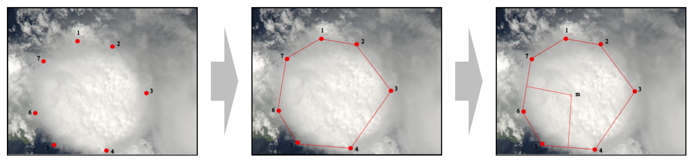
• Convex hull selection method: The convex hull selection method has lower selection complexity for irregular cloud regions. It is worth noting that this process does not require the involvement of professional annotators, thus greatly reducing labor costs.
• Minimal annotation requirements: CloudAUE achieves excellent results on using one to two annotations, which significantly reduces labor and time consumption.
• Objective evaluation criteria: CloudAUE introduces an uncertainty estimation mechanism. This novel approach establishes a criterion for terminating annotations that does not rely on human judgment, ensuring a more objective evaluation process.
• Validation of the reliability of labeled datasets: Two publicly labeled satellite image datasets are utilized to verify the effectiveness and accuracy of our proposed method. Compared with deep learning cloud detection methods, CloudAUE achieves better or competitive results without any labels.
• Extension capability in various fields: The desired results are achieved on an unlabeled forest fire dataset.

We organize this paper as follows. In Section 2, the proposed CloudAUE, the convex hull selection module, the KD-Tree module, and the uncertainty estimation module are introduced. Section 3 illustrates the experimental settings and the results on various datasets. Section 4 discusses the details of the annotation process, such as annotation areas, number of annotations, and the distribution of confidence score, followed by conclusions in Section 5.

2. Materials and Methods

In this study, the motivation of CloudAUE is to reduce the reliance on labeled samples while simultaneously mitigating the burden of manual annotation and requiring no professional knowledge. The CloudAUE method encompasses three components: The selection of training pixels module, an automatic pixel annotation module, and a quality assessment of annotations module. In the selection of training pixels module, the convex hull selection method is proposed to select cloud and non-cloud regions. In the automatic pixel annotation module, the KD-Tree classifier is applied to automatically annotate all the pixels. In the quality assessment of annotations module, an uncertainty estimation mechanism is introduced to objectively assess the quality of the annotations. When the confidence value falls below the threshold, performing secondary annotation is required to improve the quality of annotation. Figure 1 shows the flowchart of the CloudAUE method.

2.1. Sample Selection by Convex Hull

In satellite images, cloud regions typically exhibit irregular shapes. Conventional rectangular labeling methods [21] often prove inadequate in accurately delineating cloud regions, leading to a substantial number of erroneous cloud pixel annotations, which adversely impact the accuracy of the classifier in turn. For shapeless objects, polygonal regions based on a convex hull would be more suitable than conventional rectangle ones [22]. Therefore, we apply convex hull polygons to label the irregularly shaped cloud regions in satellite images. Figure 2 illustrates two convex hull polygons of annotated regions depicted in distinct colors. The red polygons correspond to the region containing cloud pixels, while the blue polygons represent the region encompassing non-cloud pixels. Training samples are generated from pixels located within these delineated regions, with pixels within the same region sharing a common label. For instance, all pixels within the red polygons are assigned the label ‘1’, whereas pixels within the blue polygons are assigned the label ‘2’ [23]. These selected pixels will be used for training the classifier. Thus, how to quickly obtain samples in the selected convex hull regions? Here, we propose a fast algorithm.

The convex hull algorithm is illustrated in Figure 3, where all samples located within the hull are utilized for the training set. How to obtain the convex hull is the key step in our proposed method. Firstly, scattered points, marked as red dots, represent pixel coordinates obtained by mouse clicks on a given image. Next, the boundary points (hull vertices) are marked with a red polygon. It is not difficult for users to identify the desired region vertices using the interactive algorithm. Lastly, since any points within the convex hull region can be linearly represented by these vertices, the algorithm makes a decision for a query point: whether it lies inside or outside the convex hull.

Assume that there are l ordered points, $z_1,z_2,\dots ,z_l$, which represent the vertices of the convex hull. The order of these points is either clockwise or anticlockwise in the same plane. Each point $z_l$ is d-dimensional, where $z_i\in {\mathbb{R}}^d$, and $i=1,2,\dots ,l$. The center of the hull, denoted as m, is defined as

$$m=\frac{1}{l}\sum _{i=1}^l{z}_i$$

(1)

Thus, the convex hull is composed of l oriented line segments, and the counterclockwise direction can be represented by vectors $z_1-z_2,z_2-z_3,\dots ,z_l-z_1$. Then, there are l projections of m to the l line segments, which are marked as $q_1,q_2,q_3,\dots ,q_l$, respectively. According to the definition of projection, the $q_i$ can be written as

$$q_i=z_i+\frac{<m-z_i,z_{i+1}-z_i>}{\parallel z_{i+1}-z_i{\parallel }^2}·(z_{i+1}-z_i),i=1,2,\dots ,l$$

(2)

where $〈·,·〉$ denotes the vector inner product, and $z_{l+1}=z_1$. Thus, our linear equation for the l segment is expressed as follows:

$$p_i^T(z-z_i)=0,i=1,2,\dots ,l$$

(3)

where $p_i=m-q_i$. The superscript T denotes vector or matrix transpose throughout the paper.

For a given query point v, the function $\lambda \left(v\right)$ is defined as follows:

$$\lambda \left(v\right)=\underset{1\le i\le l}{min}\{p_i^T(v-z_i)\}.$$

(4)

Therefore, we determine that if $\lambda >0$, the point is inside the polygon, if $\lambda =0$, it lies on the polygon, and if $\lambda <0$, it is outside the polygon. To speed up the computation, we rewrite this in matrix form. Let $Z=z_1,z_2,\dots ,z_l$ and $Q=q_1,q_2,\dots ,q_l$. For a given point v, we define the matrix as follows:

$$M=({\mathbf{1}}_l{m}^T-Q^T)(v{\mathbf{1}}_l^T-Z)$$

(5)

and

$$\lambda \left(v\right)=\underset{1\le i\le l}{min}\{diag\left(\mathbf{M}\right)\}$$

(6)

where ${\mathbf{1}}_l$ denotes the vector containing all l entries $1s$. The function $\mathrm{diag}(·)$ represents matrix diagonalization.

2.2. KD-Tree Classifier

For CloudAUE, we initially choose k-nearest neighbors (kNN) [24] for classifying each pixel. The choice of kNN is based on several advantages it offers: (1) As one of the excellent data mining algorithms, kNN has been widely popularized and applied in data classification and regression tasks. (2) Unlike many other classification methods, the operation of kNN does not rely on assumptions about the distribution of the underlying data. (3) The kNN classifier is supported by theoretical evidence that controls the error probability bounds of the two-nearest-neighbor decision rules. However, considering that most satellite images are high-resolution images, employing the KNNs algorithm might necessitate querying millions of pixels. To mitigate this computational burden, CloudAUE employs a more efficient KD-Tree [25] classifier. The KD-Tree classifier utilizes a tree structure and stores training points through axis-parallel subspace partitioning. Leveraging the inherent properties of trees, the KD-Tree classifier facilitates rapid queries within a limited search space during the construction process [26]. Indeed, for a given test sample, the process of finding the k-nearest neighbors among all training samples for traditional kNN can be replaced by querying only a subset of training samples stored in the KD-Tree. Specifically, by querying the minimum set of training points along the subtrees of the training KD-Tree, most of the search subspaces can be effectively pruned [27]. Moreover, when incorporating a new training point into an existing KD-Tree, local adjustments within the subspace to which the point belongs are sufficient. This involves traversing the tree, shifting the subspace from the root to the left or right based on the position of the point relative to the split subspace, until reaching the specified subspace containing the point.

For a given pixel input (query point), denoted as $\mathit{q}={(r,g,b)}^T$, its output label $y(\in \{1,2\})$ is determined by querying the KD-Tree constructed on the training set $\Omega$. Let $N_k\left(\mathit{q}\right)=\{{\mathit{p}}_1,{\mathit{p}}_2,\dots ,{\mathit{p}}_k\},{\mathit{p}}_i\in \Omega$ represents its first k-nearest neighbors, measured by the Euclidean distance $\parallel {\mathit{p}}_i{-\mathit{q}\parallel }_2$. The set $\{p_1,p_2,\dots ,p_k\}$, denotes their labels as $y_1,y_2,\dots ,y_k,y_i\in \{1,2\}$. In contrast to traversing all training samples, the querying process here involves traversing a small branch from the root to the cell (minimal subspace) covering q. Subsequently, backtracking from the cell to its ancestors is performed to find its k-nearest neighbors. Leveraging the KD-Tree structure, the computation is significantly more efficient than that performed in the classical kNN approach. The output y for $\mathit{q}$ can be determined by the following expression:

$$y=arg\underset{i}{max}\{\sum _{j=1}^{k}I(i==y_j)\}$$

(7)

where $I\left(x\right)$ is an indicate function and x is a logical variable; $I\left(x\right)=1$ when x is true, and 0 otherwise. The symbol ‘‘= =’’ means the logical equality. Generally speaking, Equation (7) says that $\mathit{q}$ is assigned to the class most common among its k-nearest neighbors.

2.3. Uncertainty Estimation Mechanism

When utilizing the KD-Tree classifier for obtaining annotation results $Y_{kd}$, evaluating the quality of annotation becomes crucial. Traditional annotation methods typically rely on the annotator’s subjective judgment, which can be influenced by their personalized annotation preferences. In addition, this dependence on human judgment also necessitates annotators with high professional knowledge. To address these challenges, CloudAUE introduces an objective evaluation method for assessing annotation quality. This method incorporates an uncertainty assessment mechanism to calculate the confidence value of the annotation results for each image. Once the confidence value exceeds a predefined threshold, CloudAUE automatically terminates the annotation process, and receives satisfactory annotation results. By employing this approach, CloudAUE eliminates the need for annotators with high professional knowledge, thereby significantly reducing the professional requirements for annotators. This objective evaluation method enhances the efficiency and convenience of the annotation process, making it more accessible and user friendly.

In the uncertain evaluation mechanism, CloudAUE first selects an odd number of baseline classifiers $h_1,h_2,\dots h_C$. Each baseline classifier is trained independently on the samples selected from the convex hull, and then, classifies the entire image. For each pixel $x(i,j)$ in a given image $X_{img}$, its label $y_{\mathit{comb}}(i,j)$ can be combined into C classifiers as

$$y_{\mathit{comb}}(i,j)=\mathit{Combination}\left(h_1(i,j),h_2(i,j),\dots ,h_C(i,j)\right)$$

(8)

where $(i,j)$ represents the position of a pixel in the image $X_{img}$. $h_c(i,j)$ is the prediction result of the c-th baseline classifier for the pixel of $X_{img}$ at position $(i,j)$. The function $\mathit{Combination}(·)$ is employed to aggregate the outputs of the C classifiers. Different from the traditional voting method, our approach marks pixels as clouds only if classified as such by all C classifiers, denoted by a label “1”. Similarly, pixels classified as non-clouds by all classifiers are labeled as “2”. In cases where the outputs of different classifiers diverge, the pixel is marked as “0”. Utilizing the $\mathit{Combination}(·)$ method, the input image $X_{\mathit{img}}$ yields a mask image $Y_{\mathit{img}}$ with three types of labels. To extract high-confidence reference samples, CloudAUE exclusively selects pixels labeled as “1” and “2” in $Y_{\mathit{img}}$, denoted as $Y_{\mathit{hcf}}$.

According to the pixels labeled as ’0’ in $Y_{\mathit{img}}$, the KD-Tree classifier result $Y_{\mathit{kd}}$ eliminates the corresponding pixels, resulting in an annotation subset $Y_{kdn}$. For the given image $X_{img}$, the confidence value $\mathit{Confidence}\left(X_{img}\right)$ is calculated based on the similarity between the annotation subset $Y_{kdn}$ and the high-confidence reference samples $Y_{\mathit{hcf}}$ as follows:

$$\mathit{Confidence}\left(X_{img}\right)=\frac{|Y_{kdn}-Y_{\mathit{hcf}}|}{N}$$

(9)

where N is the number of pixels in $Y_{\mathit{hcf}}$. During the annotation process, once the confidence value $\mathit{Confidence}\left(X_{img}\right)$ surpasses the threshold $\tau$, the annotation is concluded, indicating that satisfactory results have been achieved. In Section 5.3, we discuss the distribution of confidence values in detail. In a few extreme cases, when the confidence level fails to exceed the threshold after multiple annotations, CloudAUE specifies that if the confidence value does not surpass the threshold after the number of annotations exceeds 3 times that value, the annotation process will be forcibly terminated. The result with the highest confidence value among the three annotations is then selected as the final result.

3. Experimental Settings

3.1. Dataset

Two labeled datasets, the HRC dataset and the Landsat 8 dataset, are used to verify the effectiveness of our method. In addition, an unlabeled dataset is constructed to demonstrate its availability and ease of use.

The HRC dataset, a high-resolution cloud cover validation dataset, was created by the SENDIMAGE Laboratory of Wuhan University. All images are annotated by remote sensing experts. This dataset consists of 150 high-resolution images acquired through three RGB channels with resolutions ranging from 0.5 to 15 m. These images contain five land cover types, namely, water bodies, vegetation, wetlands, urban, snow/ice, and barren [28].

The operational land imager (OLI) optical sensor of Landsat 8 contains nine spectral bands. In this study, three of these common bands are selected, band 2 (blue), band 3 (green), and band 4 (red), to form three RGB-channel images. Then, a gradient-based identification method is applied to identify and exclude snow/ice regions from the ground truth of the training set. In this way, a corrected and more accurate binary cloud mask can be obtained. After the above preprocessing, the Landsat 8 cloud dataset contains 31 satellite images divided into 23 training images and 8 test images. The ground truth (gt) of all these images is manually annotated pixel by pixel. The Landsat 8 spectral band image is approximately 5000 × 5000 pixels [16].

In order to construct an unlabeled dataset, we randomly selected a collection of four remote sensing satellite images from Google Earth, without pre-established labels. This satellite has a spatial resolution of 30 m and an orbital altitude of 705 km above sea level. These four images contain the most common terrains from the eastern and central regions of Asia, and are at a resolution of 1100 × 966. At the same time, the cloud types include from scattered clouds to whole clouds, and from thin clouds to thick clouds.

3.2. Experimental Settings

In order to evaluate CloudAUE, we select three approaches based on deep learning technology, which include two classical semantic segmentation methods, UNet [29] and Deeplabv3+ [30], and one recent cloud detection method, Cloud-AttU. Cloud-AttU is based on the UNet architecture with attention mechanism. During the training phase of the three compared methods, the batch size is 4 and the epoch is 50. The learning rate and momentum of RMSProp are 0.0001 and 0.9, respectively. Due to the large pixel size of the images in the Landsat 8 dataset, each image is cropped into 384 × 384 non-overlapping patches. The training and testing datasets contain 3543 and 1352 patches, respectively. For the HRC dataset, 120 and 30 images are utilized to train and test, respectively. Notably, CloudAUE uses a set of pixels selected from convex hulls to train the classifier, and does not require setting up training and testing sets as traditional deep learning methods. Thus, the division of training and testing data for the two datasets is only for the three compared methods.

In the quality assessment of annotations module, CloudAUE proposes an uncertainty estimation mechanism, which needs to choose odd base classifiers. Here, three classifiers, including support vector machine (SVM), discriminant analysis, and random forest, are selected. Through the ensemble the classification results, a high-confidence mask of clouds is obtained. The threshold value $\tau$ is set to 80%. When the confidence value reaches 80%, it means that the annotation quality is sufficient and can be stopped. In addition, if the number of annotations reaches three but the threshold value still does not reach 80%, we can stop annotating the image.

3.3. Evaluation Metrics

Within the experiment, the predicted cloud coverage was categorized into two classes: cloud and non-cloud. Consequently, the accuracy assessment aims to measure the consistency between cloud and non-cloud in the predicted mask and ground truths at the pixel level. The evaluation metrics are employed to compare our model with three comparisons, included the Jaccard index, accuracy, recall rate, specificity, F1 score, and overall accuracy [31]. The definitions of the six metrics are elaborated upon as follows:

$$JaccardIndex=\frac{TP}{TP+FN+FP}$$

(10)

$$Precision=\frac{TP}{TP+FP}$$

(11)

$$Recall=\frac{TP}{TP+FN}$$

(12)

$$Specificity=\frac{TN}{TN+FP}$$

(13)

$$F_1=\frac{2precisionrecall}{precision+recall}$$

(14)

$$OverallAccuracy=\frac{TP+TN}{TP+TN+FP+FN}$$

(15)

where TP, TN, FP, and FN represent true positive, true negative, false positive, and false negative pixels, representing the number of correctly detected cloud pixels, the number of correctly detected non-cloud pixels, the number of false alarm pixels, and the number of missed cloud pixels, respectively. A larger measurement means a more exact Jaccard index, also known as the intersection over union (IoU) [32], which emphasizes the set of similarities between two samples and is one of the most commonly used metrics in image semantic segmentation tasks [33]. Accuracy is the total number of correctly classified cloud pixels divided by the total number of cloud pixels. Precision reflects the proportion of positive identification of the cloud that is correct, while “recall” determines the proportion of actual positives that are correctly identified [34]. The F1 score combines precision and recall [35]. Note that the Jaccard index, F1 score, and overall accuracy are comprehensive indicators.

4. Results

To validate the effectiveness of our proposed model, we compare CloudAUE with UNet, Deeplabv3+, and Cloud-AttU on the HRC and Landsat 8 datasets with labels of each pixel. Then, the Google Earth dataset without labels is utilized to show the availability and ease of use of CloudAUE.

4.1. Results on the HRC Dataset

The quantitative results of CloudAUE and the three compared models on the HRC dataset are listed in

Table 1. Performance of various methods on HRC dataset.

Method	Jaccard	Precision	Recall	Specificity	F1	Accuracy
UNet	66.63	88.55	76.18	92.80	78.47	86.16
Deeplabv3+	64.94	80.35	80.55	85.82	77.10	82.37
Cloud-AttU	69.83	86.26	81.43	90.19	80.34	87.03
CloudAUE	74.89	87.85	88.86	93.80	87.92	93.06

. From Table 1, CloudAUE achieves better performance compared to the three deep learning methods, except for on precision. The Jaccard index, F1 score, and accuracy of CloudAUE are 5.04%, 7.58%, and 6.03% higher than Cloud-AttU which obtains the second best performance, respectively. These three comprehensive indicators are most important in cloud detection. In addition, as can be seen from the table, Cloud-AttU incorporating the attention mechanism is superior to the two classical segmentation methods on the HRC dataset.

Then, two images from the testing dataset are selected for qualitative analysis of a single image. The first selected image has forest background covered by thick clouds. Figure 4 shows the qualitative results of the various methods. The annotation areas of CloudAUE are marked in Figure 4a, with red polygons selecting thick cloud regions and blue polygons selecting forest regions. From Figure 4, it can be seen that CloudAUE performs better in the detailed parts of clouds. In the bottom right corner, Deeplabv3+ incorrectly detects the forest area as part of the clouds; see Figure 4e. In the top right corner, Cloud-AttU mistakenly identifies some scattered clouds; see Figure 4f. In addition,

Table 2. The quantitative results of the various methods on an image covered by thick clouds.

Method	Jaccard	Precision	Recall	Specificity	F1	Accuracy
UNet	87.99	99.49	88.39	99.82	93.61	96.54
Deeplabv3+	84.23	94.05	88.96	97.74	91.44	95.22
Cloud-AttU	89.62	94.67	94.37	97.86	94.52	96.86
CloudAUE	90.38	97.83	92.22	99.18	94.95	97.19

presents the quantitative results of the various methods on this image. Since thick clouds are detected easily, CloudAUE and the three compared methods obtain good results. And CloudAUE obtains the highest Jaccard index, F1 scores, and accuracy.

The second selected images have a barren land background covered by thin clouds. Similar to the analysis of the above image, Figure 5 displays the qualitative results of the different approaches. The red and blue polygons select thin cloud and barren land regions, respectively, as shown in Figure 5a. In the middle part, the three deep learning methods misclassify thin clouds as wasteland, resulting in cloud pixels being incorrectly identified as non-cloud pixels. This seriously affects the performances of the three compared methods. However, the CloudAUE method is able to detect most of these thin cloud regions, and receives excellent detection results.

Table 3. The quantitative results of the various methods on an image covered by thin clouds.

Method	Jaccard	Precision	Recall	Specificity	F1	Accuracy
UNet	68.23	99.80	68.32	99.87	81.11	84.53
Deeplabv3+	57.38	97.16	58.36	98.38	72.92	78.93
Cloud-AttU	78.13	99.83	78.23	99.87	87.72	89.35
CloudAUE	87.76	93.34	93.62	93.68	93.48	93.65

shows the quantitative results of the various approaches. It is worth noting that the Jaccard metric of CloudAUE is significantly better than the three deep learning methods, achieving an impressive 87.76% for thin cloud detection. In addition, the overall accuracy, F1 score, and recall of CloudAUE reach 93.65%, 93.48%, and 93.62%, respectively, and also exceed the compared methods. These results show that CloudAUE can achieve excellent performance for detecting thin clouds.

Since the ground type in remote sensing images directly affects the performance of cloud annotation, we partitioned the background into eight distinct types: forest, water, snow, barren land, shrubland, urban, agriculture, and mountain [36]. Then, the six evaluation metrics of CloudAUE were calculated on the eight background types, and the results are listed in

Table 4. The performance of CloudAUE on eight background types.

Scene	Jaccard	Precision	Recall	Specificity	F1	Accuracy
Forest	90.49	95.29	94.68	96.06	94.89	96.38
Water	76.70	91.30	82.84	96.17	86.24	94.66
Snow	58.36	67.20	81.81	87.13	73.06	86.06
Barren land	83.93	94.27	88.54	96.65	91.21	95.95
Agriculture	92.04	98.06	93.78	97.94	95.85	96.06
Shrubland	92.79	95.39	97.14	94.96	96.26	96.11
Urban	76.34	86.91	85.17	94.65	85.82	93.86
Mountain	87.53	94.38	92.47	92.54	93.30	92.08

. From the table, CloudAUE receives the highest Jaccard index on the shrubland type, which reaches 92.79%. On the forest and agriculture types, CloudAUE also exceeds a 90% Jaccard index. At the same time, CloudAUE achieves the top three results in F1 score and overall accuracy on the shrubland, forest, and agriculture types. However, CloudAUE obtains the lowest values for all six metrics on the snowy background type, obviously worse than other background types. Due to the similar colors, it is very difficult to distinguish snow and clouds, even by manual labeling. These results indicate that CloudAUE can obtain excellent performance when the background is a single type and greatly differs from the clouds.

To further evaluate CloudAUE on the eight background types, Figure 6 shows the six metrics for CloudAUE and the three deep learning methods. The size of the octagon in each subfigure correlates with the performances of each method on the corresponding metric, with larger octagons indicating better performance. As can be seen from the figure, CloudAUE has the largest octagons in each subfigure, meaning it shows significant improvements compared with three deep learning methods. Notably, in the snowy background, where cloud detection is challenging, all three compared methods also achieve very poor performance, scoring around 40% on the Jaccard index.

4.2. Results of Landsat 8 Dataset

To additionally assess the effectiveness of CloudAUE,

Table 5. Performance of the various methods on Landsat 8 dataset.

Method	Jaccard	Precision	Recall	Specificity	F1	Accuracy
UNet	83.02	90.72	90.73	84.55	90.72	88.41
Deeplabv3+	81.31	87.57	91.92	80.81	89.69	87.42
Cloud-AttU	83.26	90.17	91.58	84.04	90.87	88.67
CloudAUE	79.87	91.11	82.06	87.34	85.82	89.56

provides the performance of the various methods on the Landsat 8 dataset. As is evident from the table, CloudAUE achieves the highest overall accuracy and precision, attaining 89.56% and 91.11%, respectively. But it performs slightly worse on the Jaccard index and F1 score. Due to the large pixel size of the images in the Landsat 8 dataset, the three deep learning methods typically partition these images into smaller patches for training, enabling better learning of both local and global features. However, CloudAUE directly annotates only one cloud and non-cloud region on the original-sized image, potentially resulting in the loss of global features and a decrease in accuracy. Nevertheless, our method still achieves competitive results without requiring any labels, as compared to the deep learning methods.

It is notable that CloudAUE achieves excellent performance on detecting thin clouds in the HRC dataset. Here, we choose an image covered by thin clouds to validate this ability of CloudAUE again. Figure 7 shows the qualitative results of the different methods on this image. As can be seen from the right half of Figure 7, the three compared methods tend to excessively detect the background as clouds, but CloudAUE obviously reduces the misjudgment of the background.

In cloud detection tasks, identifying scattered clouds poses a significant challenge. Hence, we select an image covered with scattered clouds to evaluate the effectiveness of our proposed method. Figure 8 illustrates the qualitative results of the various methods. In Figure 8a, red and blue polygons indicate cloud and non-cloud annotation areas, respectively. As depicted in the figure, CloudAUE demonstrates accurate detection of the scattered clouds, whereas other methods mistakenly identify the large background in the upper left corner as clouds.

4.3. Results on Self-Built Google Earth Dataset

The above two datasets, with pixel-level labels, are utilized to quantitatively assess the accuracy of our method. However, when a new satellite produces a large number of remote sensing images without any labels, deep learning methods face challenges in training models on this new dataset. Even with transfer learning technology, the detection performance may significantly decrease. The advantage of CloudAUE is that it does not require any labels for cloud detection. Here, we utilize a self-built Google Earth dataset without labels to validate the effectiveness of our method. The four remote sensing images contain various types of clouds and backgrounds, such as scattered and thin clouds, forests, water, and wasteland, as depicted in Figure 9a. Next, red and blue polygons are annotated to designate cloud and non-cloud regions in Figure 9b. CloudAUE employs uncertainty estimation to determine whether the expected quantity of cloud annotations is attained. When the confidence value surpasses 80%, the annotation process halts, and the final annotation results are deemed satisfactory. Figure 9c illustrates the final annotation outcomes. The four images, from top to bottom, only require annotation once, with confidence values exceeding 80%, reaching 84.3%, 85.34%, 88.32%, and 82.41%, respectively. Due to the absence of labels, the annotation results cannot be quantitatively analyzed. Nevertheless, based on visual inspection, CloudAUE successfully detects different types of clouds across various background types, and the annotation results are deemed acceptable.

4.4. Expanding Capabilities to Forest Fire Dataset

The CloudAUE method has successfully demonstrated its efficacy in cloud detection within remote sensing images. In order to further explore the expanding capabilities on automatic annotation in diverse fields, we selected an unlabeled forest fire dataset, which encompasses forest fire images with close- or long-range background under different light conditions [23]. The four fire images represent scenes from long-range to close-range backgrounds from top to bottom in Figure 10a. Then, red and blue polygons are annotated to designate fire and non-fire regions in Figure 10b. Given the increased complexity of the backgrounds in the forest fire images compared to remote sensing imagery, we suggest that non-fire regions, delineated by selecting blue polygons, should ideally incorporate multiple distinct backgrounds simultaneously. These backgrounds may include trees, mountains, vegetation, or any other elements commonly found in forested environments. By encompassing diverse backgrounds within non-fire regions, CloudAUE can obtain a more comprehensive representation of the surrounding environment. Figure 10c shows the final annotation results. All four images only needed to be annotated once and their confidence values exceed 80%. The confidence values for the four images, from top to bottom, are 88.13%, 88.21%, 80.32%, and 82.42%, respectively. This indicates that the annotation results have met the desired performance. Additionally, through visual inspection, comparing the original images with the annotation results it is evident that our proposed method effectively distinguishes between fire and non-fire regions. These experimental results on the forest fire dataset show that CloudAUE has strong expansion capabilities for automatic annotation in different fields.

5. Discussion

The annotated area plays a pivotal role in the accuracy of CloudAUE. Additionally, there exists a correlation between the number of annotations and the confidence threshold, which indirectly impacts the performance of CloudAUE. Therefore, we will explore strategies for selecting annotated areas, determining the appropriate number of annotations, and setting the optimal confidence threshold.

5.1. Selection of Annotation Areas

In order to research the impact of the selection of annotation areas on the performance of CloudAUE, an image covered with thin clouds is chosen from the HRC dataset. Next, we perform two completely different selections of annotation areas.

As depicted in Figure 11a, the red polygon selects relatively transparent thin cloud regions as cloud samples, while the blue polygon selects the barren background as non-cloud samples. After the initial classification, the annotated results are shown in Figure 11b. It is evident that a considerable number of thin clouds are misclassified as background features, with only slightly thicker clouds retained. From the first row of

Table 6. The confidence level and six metrics of different annotation areas.

Selection	Confidence	Jaccard	Precision	Recall	Specificity	F1	Accuracy
First (Figure 11a)	0.73	0.69	0.99	0.69	0.99	0.82	0.85
Second (Figure 11c)	0.82	0.89	0.92	0.96	0.93	0.94	0.94

, the confidence value is only 73%, falling below the threshold of 80%. In such cases, a second annotation or reselection of annotation areas is necessary. In Figure 11c, an alternative selection of annotation areas is provided, avoiding the thin cloud regions. Consequently, the red polygon selects slightly thicker cloud regions, while the blue polygon continues to select the barren background. The annotated results are displayed in Figure 11d. Compared with the misidentification of the first annotation strategy, thin cloud regions in the middle part of the image are now clearly detected. In the second row of Table 6, the confidence value increases by 9%, reaching 82%, exceeding the threshold of 80%. The Jaccard index, F1 score, and overall accuracy also show noticeable improvements. Therefore, satisfactory results can be obtained with just one annotation.

Based on the experiments conducted and our accumulated experience, we offer some recommendations for selecting annotation areas:

• Red polygon (cloud regions):

  *

  Optimal choices for thick cloud regions;

  *

  Avoid thin cloud regions to ensure accurate delineation of cloud regions.

• Blue polygon (non-cloud regions):

  *

  Ensure that annotation areas chosen are distinctly different from cloud regions;

  *

  When dealing with backgrounds comprising two types, consider selecting areas that represent the intersection of both background types. This strategy ensures that the annotated areas capture the common characteristics shared by both background types.

Following these suggestions can contribute to more accurate annotation, and consequently, enhance the performance of cloud detection algorithms.

5.2. Number of Annotations

CloudAUE firstly delineates cloud and non-cloud areas using two polygons, then utilizes an uncertainty estimation to assess the annotation quality. If the confidence values fail to exceed the threshold of 80%, the second annotation becomes necessary to improve confidence. Unlike the first annotation, the second annotation exclusively selects non-cloud areas using a polygon, ensuring maximal dissimilarity from the non-cloud areas selected by the first annotation. Up until the third annotation, if the confidence value fails to reach the threshold of 80%, the entire annotation process will be terminated, and the result of the third annotation becomes the final outcome. CloudAUE aims to reduce the number of annotations, thereby lowering annotation costs. Here, we delve into a detailed analysis of the impact of the number of annotations on performance.

In Figure 11, the histograms display the distribution of the number of annotations for each image in both the HRC and Landsat 8 datasets. As depicted in the figure, approximately 67.3% and 77.4% of the images require only one annotation, with their confidence levels exceeding 80%, resulting in acceptable outcomes. On average, the entirety of the HRC and Landsat 8 datasets requires only 1.43 and 1.25 annotations, respectively. Furthermore, sixteen and one images are annotated three times, indicating that the final confidence values of these images still do not exceed the threshold of 80%. However, the maximum number of annotations (three times) is reached, leading to termination of the annotation processes. It is worth noting that these images share a common feature—the background is snow. In cloud detection tasks, distinguishing between snow and clouds remains a significant challenge.

5.3. The Distribution of Confidence Values

CloudAUE utilizes the uncertainty evaluation method to compute the confidence value for each image, serving as a metric to assess the quality of the annotation results. Further discussion on the distribution of confidence values aids in selecting an appropriate threshold, $\tau$. Upon obtaining results for the HRC and Landsat 8 datasets as shown in Table 1 and Table 5, the distribution of confidence values is depicted in Figure 12. Notably, approximately 90% and 96.8% of the images in both datasets exhibit confidence values exceeding 80%. Corresponding to Figure 13, most of the images require only one annotation to achieve a confidence level exceeding 80%. However, there are a few images with confidence levels below 80%, despite undergoing at least three annotations. The annotation processes are terminated because they do not exceed the threshold. The common feature of these images is that the background is snow. Due to the difficulty in distinguishing between snow and clouds in the background, more annotations do not significantly improve the confidence value due to this inherent challenge.

Based on the analysis of the confidence distribution on the HRC and Landsat 8 datasets, a threshold of 80% is chosen for assessing the quality of annotation results in this article. However, it is important to note that this threshold can be adjusted based on the characteristics of the dataset. For datasets with a single background type and no snow background, the threshold can be increased to enhance annotation quality. This higher threshold ensures that annotations are more accurate and reliable, given the relative simplicity of the dataset. Conversely, for datasets with complex backgrounds containing snow, lowering the threshold may be beneficial to reduce the number of annotations while still achieving acceptable annotation quality. Ultimately, adjusting the threshold according to dataset characteristics allows for better optimization of the annotation process and ensures more effective cloud annotation.

5.4. The Balance between Performance and the Number of Annotations

The regular annotation process of CloudAUE involves terminating the annotation process when an image is annotated once and its confidence value exceeds the threshold. However, irrespective of efficiency considerations, can users improve the quality of annotation by infinitely increasing the number of annotations? To explore this, we select two images from the HRC dataset, both of which are covered by thick clouds, but the background types are complex urban background and simple agricultural background. Figure 14 and

Table 7. Performance of number of annotations on an urban background image.

Number	Jaccard	Precision	Recall	Specificity	F1	Accuracy
First (Figure 14b)	79.16	85.07	91.92	91.23	83.58	86.57
Second (Figure 14c)	82.64	90.35	90.63	94.73	90.49	93.29
Third (Figure 14d)	76.46	95.50	79.31	91.76	86.66	91.39

present the qualitative and quantitative results of multiple annotations of an urban background image. In Figure 14a, the cloud and non-cloud areas are initially selected by red and blue polygons in the original image during the first annotation. Subsequently, Figure 14b displays the result of the first annotation, where the confidence value exceeds the threshold of 80%. However, due to the complex urban background, the roofs of buildings are misidentified as clouds. Thus, the second annotation selects these roofs using the blue polygon. Figure 14c illustrates the result of the second annotation. Here, it is evident that most outlines of urban buildings in the background are accurately detected as non-cloud. Table 7 also indicates slight improvements in three comprehensive metrics: Jaccard index, F1 score, and overall accuracy. Subsequently, the blue polygon in Figure 14c undergoes annotation for the third time, and the results are displayed in Figure 14d. From Figure 14d, the thin clouds on the outlines of clouds are misidentified as background. Table 7 also shows significant drops in the metrics marked for the third time compared to the second time.

Figure 15 and

Table 8. Performance of number of annotations on an agriculture background image.

Number	Jaccard	Precision	Recall	Specificity	F1	Accuracy
First (Figure 15b)	90.76	95.45	94.79	96.91	95.12	96.05
Second (Figure 15c)	93.57	98.73	94.76	99.16	96.67	97.35
Third (Figure 15d)	91.35	99.64	91.80	99.77	95.56	96.53

display multiple annotation results for an agricultural background, where the background is relatively singular. Similarly, after the first annotation, the confidence value exceeds the threshold of 80%. However, there is a long white strip on the ground in the upper right corner of Figure 15b, which is detected as cloud. Therefore, during the second annotation, the blue polygon needs to select this part. Figure 15c illustrates the result after the second annotation, where the white ground that is previously regarded as clouds is correctly classified as background. Table 8 also demonstrates that the performance of the second annotation slightly improves. However, when Figure 15c is annotated for the third time, it can be observed from Figure 15d that the thin clouds on the cloud outline are detected as background, leading to performance degradation, as shown in Table 8.

The experimental results demonstrate that continuously increasing the number of annotations does not necessarily lead to continuous improvement in annotation performance. Generally speaking, once the confidence value exceeds the threshold after the first annotation, if efficiency is not a concern, conducting a second annotation may be beneficial to achieve optimized results. However, there is usually no need to perform a third annotation. Over-annotation can lead to the outline of the cloud being misclassified as the background, thereby reducing the performance of CloudAUE annotation. In practical operation, it is advisable for users to terminate the annotation process once the annotation confidence value surpasses the threshold, without the need for further annotations. This strategy helps strike a balance between performance and the number of annotations while still achieving satisfactory annotation quality.

6. Conclusions

To address the dependence on labeled datasets and professional domain knowledge in traditional cloud annotation methods, this paper proposes an automatic cloud annotation method, CloudAUE, for satellite remote sensing images. CloudAUE can be operated interactively by users without domain knowledge. Due to the irregular shapes of clouds, two polygons are utilized to select cloud and non-cloud regions. By selecting the vertices of the cloud and non-cloud polygons in turn, the whole region is accurately selected to obtain reliable cloud pixels and non-cloud pixels. Then, each pixel is classified by the KD-Tree algorithm. Finally, the quality of the annotation results is evaluated using the confidence value of the image through an uncertainty estimation mechanism. Once the confidence value of an image surpasses the 80% threshold, the annotation process halts and obtains satisfactory results. Conversely, if the confidence value drops below the threshold, the image requires a second annotation. On the labeled HRC and Landsat 8 datasets, CloudAUE exhibits comparable or superior accuracy when compared to three deep learning algorithms, and performs better on thin and scattered clouds. When the above performance is obtained, the average number of annotations are 1.43 and 1.25, respectively. Moreover, the annotation results on the unlabeled self-built Google Earth dataset and fire forest dataset demonstrate the effectiveness and expanding capabilities of CloudAUE. In further analysis, we provide some suggestions for annotation regions to help improve annotation results and reduce the number of annotations. And telling users to continually increase the number of annotations does not necessarily lead to ever-increasing annotation performance.

In future endeavors, we can explore optimizing the annotation process with CloudAUE by initially clustering similar images into subsets [37]. By selecting and annotating a representative image within each subset, we can leverage the annotation model to automatically annotate the remaining images in the same subset. This approach promises to significantly enhance annotation efficiency. The other direction is that integrating active learning methodologies can further elevate annotation performance [38]. Furthermore, CloudAUE can be deemed as a general automatic annotation tool to expand to other fields, such as forest area detection, forest vegetation detection, etc.

References

1. Sawaya, K.E.; Olmanson, L.G.; Heinert, N.J.; Brezonik, P.L.; Bauer, M.E. Extending satellite remote sensing to local scales: Land and water resource monitoring using high-resolution imagery. Remote Sens. Environ. 2003, 88, 144–156. [Google Scholar] [CrossRef]
2. Shao, M.; Zou, Y. Multi-spectral cloud detection based on a multi-dimensional and multi-grained dense cascade forest. J. Appl. Remote Sens. 2021, 15, 028507. [Google Scholar] [CrossRef]
3. Schiffer, R.A.; Rossow, W.B. The International Satellite Cloud Climatology Project (ISCCP): The first project of the world climate research programme. Bull. Am. Meteorol. Soc. 1983, 64, 779–784. [Google Scholar] [CrossRef]
4. Schmit, T.J.; Lindstrom, S.S.; Gerth, J.J.; Gunshor, M.M. Applications of the 16 spectral bands on the Advanced Baseline Imager (ABI). J. Oper. Meteorol. 2018, 6, 33–46. [Google Scholar] [CrossRef]
5. Zhu, Z.; Woodcock, C.E. Object-based cloud and cloud shadow detection in Landsat imagery. Remote Sens. Environ. 2012, 118, 83–94. [Google Scholar] [CrossRef]
6. Shang, H.; Letu, H.; Xu, R.; Wei, L.; Wu, L.; Shao, J.; Nagao, T.M.; Nakajima, T.Y.; Riedi, J.; He, J.; et al. A hybrid cloud detection and cloud phase classification algorithm using classic threshold-based tests and extra randomized tree model. Remote Sens. Environ. 2024, 302, 113957. [Google Scholar] [CrossRef]
7. LeCun, Y.; Bengio, Y.; Hinton, G. Deep learning. Nature 2015, 521, 436–444. [Google Scholar] [CrossRef] [PubMed]
8. Zhang, L.; Wang, M.; Liu, M.; Zhang, D. A survey on deep learning for neuroimaging-based brain disorder analysis. Front. Neurosci. 2020, 14, 779. [Google Scholar] [CrossRef]
9. Fang, Y.; Ye, Q.; Sun, L.; Zheng, Y.; Wu, Z. Multi-attention joint convolution feature representation with lightweight transformer for hyperspectral image classification. IEEE Trans. Geosci. Remote. Sens. 2023, 61, 1–14. [Google Scholar]
10. Li, L.; Li, X.; Jiang, L.; Su, X.; Chen, F. A review on deep learning techniques for cloud detection methodologies and challenges. Signal Image Video Process. 2021, 15, 1527–1535. [Google Scholar] [CrossRef]
11. Shao, Z.; Pan, Y.; Diao, C.; Cai, J. Cloud detection in remote sensing images based on multiscale features-convolutional neural network. IEEE Trans. Geosci. Remote Sens. 2019, 57, 4062–4076. [Google Scholar] [CrossRef]
12. Francis, A.; Sidiropoulos, P.; Muller, J.P. CloudFCN: Accurate and robust cloud detection for satellite imagery with deep learning. Remote Sens. 2019, 11, 2312. [Google Scholar] [CrossRef]
13. Jeppesen, J.H.; Jacobsen, R.H.; Inceoglu, F.; Toftegaard, T.S. A cloud detection algorithm for satellite imagery based on deep learning. Remote Sens. Environ. 2019, 229, 247–259. [Google Scholar] [CrossRef]
14. Mohajerani, S.; Saeedi, P. Cloud-Net: An end-to-end cloud detection algorithm for Landsat 8 imagery. In Proceedings of the IGARSS 2019-2019 IEEE International Geoscience and Remote Sensing Symposium, Yokohama, Japan, 28 July 2019–2 August 2019; IEEE: Piscataway, NJ, USA, 2019; pp. 1029–1032. [Google Scholar]
15. Guo, Y.; Cao, X.; Liu, B.; Gao, M. Cloud detection for satellite imagery using attention-based U-Net convolutional neural network. Symmetry 2020, 12, 1056. [Google Scholar] [CrossRef]
16. Zhang, L.; Sun, J.; Yang, X.; Jiang, R.; Ye, Q. Improving deep learning-based cloud detection for satellite images with attention mechanism. IEEE Geosci. Remote Sens. Lett. 2021, 19, 1–5. [Google Scholar] [CrossRef]
17. Ge, W.; Yang, X.; Jiang, R.; Shao, W.; Zhang, L. CD-CTFM: A Lightweight CNN-Transformer Network for Remote Sensing Cloud Detection Fusing Multiscale Features. IEEE J. Sel. Top. Appl. Earth Obs. Remote. Sens. 2024, 17, 4538–4551. [Google Scholar] [CrossRef]
18. Zhang, B.; Zhang, Y.; Li, Y.; Wan, Y.; Yao, Y. CloudViT: A lightweight vision transformer network for remote sensing cloud detection. IEEE Geosci. Remote Sens. Lett. 2022, 20, 1–5. [Google Scholar] [CrossRef]
19. Tymchenko, B.; Marchenko, P.; Spodarets, D. Segmentation of cloud organization patterns from satellite images using deep neural networks. Her. Adv. Inf. Technol. 2020, 1, 352–361. [Google Scholar] [CrossRef]
20. Iglovikov, V.; Mushinskiy, S.; Osin, V. Satellite imagery feature detection using deep convolutional neural network: A kaggle competition. arXiv 2017, arXiv:1706.06169. [Google Scholar]
21. Luboschik, M.; Schumann, H.; Cords, H. Particle-based labeling: Fast point-feature labeling without obscuring other visual features. IEEE Trans. Vis. Comput. Graph. 2008, 14, 1237–1244. [Google Scholar] [CrossRef]
22. Mingqiang, Y.; Kidiyo, K.; Joseph, R. A survey of shape feature extraction techniques. Pattern Recognit. 2008, 15, 43–90. [Google Scholar]
23. Yang, X.; Chen, R.; Zhang, F.; Zhang, L.; Fan, X.; Ye, Q.; Fu, L. Pixel-level automatic annotation for forest fire image. Eng. Appl. Artif. Intell. 2021, 104, 104353. [Google Scholar] [CrossRef]
24. Cariou, C.; Le Moan, S.; Chehdi, K. Improving K-nearest neighbor approaches for density-based pixel clustering in hyperspectral remote sensing images. Remote Sens. 2020, 12, 3745. [Google Scholar] [CrossRef]
25. Zhang, J.; Shi, H. Kd-tree based efficient ensemble classification algorithm for imbalanced learning. In Proceedings of the 2019 International Conference on Machine Learning, Big Data and Business Intelligence (MLBDBI), Taiyuan, China, 8–10 November 2019; IEEE: Piscataway, NJ, USA, 2019; pp. 203–207. [Google Scholar]
26. Mahadik, S.M.; Kokate, S.M. A Survey on Fast nearest Neighbor Search Using KD Tree and Inverted Files. Int. J. Adv. Res. Comput. Sci. Manag. Stud. 2015, 3, 332–336. [Google Scholar]
27. Maneewongvatana, S.; Mount, D.M. An empirical study of a new approach to nearest neighbor searching. In Proceedings of the Workshop on Algorithm Engineering and Experimentation, Washington, DC, USA, 5–6 January 2001; Springer: Berlin/Heidelberg, Germany, 2001; pp. 172–187. [Google Scholar]
28. Li, Z.; Shen, H.; Cheng, Q.; Liu, Y.; You, S.; He, Z. Deep learning based cloud detection for remote sensing images by the fusion of multi-scale convolutional features. arXiv 2018, arXiv:1810.05801. [Google Scholar]
29. Ronneberger, O.; Fischer, P.; Brox, T. U-net: Convolutional networks for biomedical image segmentation. In Medical Image Computing and Computer-Assisted Intervention—MICCAI 2015, Proceedings of the 18th International Conference, Munich, Germany, 5–9 October 2015; Proceedings, Part III 18; Springer: Piscataway, NJ, USA, 2015; pp. 234–241. [Google Scholar]
30. Chen, L.C.; Zhu, Y.; Papandreou, G.; Schroff, F.; Adam, H. Encoder-decoder with atrous separable convolution for semantic image segmentation. In Proceedings of the European Conference on Computer Vision (ECCV), Munich, Germany, 8–14 September 2018; pp. 801–818. [Google Scholar]
31. Kanu, S.; Khoja, R.; Lal, S.; Raghavendra, B.; Asha, C. CloudX-net: A robust encoder-decoder architecture for cloud detection from satellite remote sensing images. Remote Sens. Appl. Soc. Environ. 2020, 20, 100417. [Google Scholar] [CrossRef]
32. Ogwok, D.; Ehlers, E.M. Jaccard index in ensemble image segmentation: An approach. In Proceedings of the 2022 5th International Conference on Computational Intelligence and Intelligent Systems, Quzhou, China, 4–6 November 2022; pp. 9–14. [Google Scholar]
33. Garcia-Garcia, A.; Orts-Escolano, S.; Oprea, S.; Villena-Martinez, V.; Martinez-Gonzalez, P.; Garcia-Rodriguez, J. A survey on deep learning techniques for image and video semantic segmentation. Appl. Soft Comput. 2018, 70, 41–65. [Google Scholar] [CrossRef]
34. Powers, D.M. Evaluation: From precision, recall and F-measure to ROC, informedness, markedness and correlation. arXiv 2020, arXiv:2010.16061. [Google Scholar]
35. Chicco, D.; Jurman, G. The advantages of the Matthews correlation coefficient (MCC) over F1 score and accuracy in binary classification evaluation. BMC Genom. 2020, 21, 6. [Google Scholar] [CrossRef]
36. Wang, J.; Yang, D.; Chen, S.; Zhu, X.; Wu, S.; Bogonovich, M.; Guo, Z.; Zhu, Z.; Wu, J. Automatic cloud and cloud shadow detection in tropical areas for PlanetScope satellite images. Remote Sens. Environ. 2021, 264, 112604. [Google Scholar] [CrossRef]
37. Lee, Y.J.; Grauman, K. Foreground focus: Unsupervised learning from partially matching images. Int. J. Comput. Vis. 2009, 85, 143–166. [Google Scholar] [CrossRef]
38. Budd, S.; Robinson, E.C.; Kainz, B. A survey on active learning and human-in-the-loop deep learning for medical image analysis. Med. Image Anal. 2021, 71, 102062. [Google Scholar] [CrossRef]
Figure 1. Cloud detection automatic annotation flowchart.
Fire 07 00212 g001
Figure 2. Illustration of two convex hulls on satellite image, marked with colored polygons.
Fire 07 00212 g002
Figure 3. Illustration of the convex hull algorithm.
Fire 07 00212 g003
Figure 4. The qualitative results of the various methods on an image covered by thick clouds. Red and blue polygons are annotation areas of CloudAUE for cloud and non-cloud regions, respectively.
Fire 07 00212 g004
Figure 5. The qualitative results of the various methods on an image covered by thin clouds.
Fire 07 00212 g005
Figure 6. Performance of various methods on eight background types. Green octagon represents CloudAUE. Red, blue, and orange octagons represent UNet, Deeplabv3+, and Cloud-AttU, respectively.
Fire 07 00212 g006
Figure 7. The qualitative results of the various methods on an image covered with thin clouds from Landsat 8 dataset.
Fire 07 00212 g007
Figure 8. The qualitative results of various methods on an image covered with scattered clouds from Landsat 8 dataset.
Fire 07 00212 g008
Figure 9. Annotation results of CloudAUE on self-built Google Earth dataset.
Fire 07 00212 g009
Figure 10. Annotation results of CloudAUE on a forest fire dataset.
Fire 07 00212 g010
Figure 11. Two different selections of annotation areas and corresponding annotation results.
Fire 07 00212 g011
Figure 12. The distribution of confidence values on the HRC and Landsat 8 datasets.
Fire 07 00212 g012
Figure 13. The number of annotations on the HRC and Landsat 8 datasets.
Fire 07 00212 g013
Figure 14. The qualitative results of number of annotations on an urban background image. (a) Original image and the first annotation areas. (b) Result of the first annotation and the second annotation areas. (c) Result of the second annotation and the third annotation areas. (d) Result of the third annotation.
Fire 07 00212 g014
Figure 15. The qualitative results of the number of annotations on an agriculture image. (a) Original image and the first annotation areas. (b) Result of the first annotation and the second annotation areas. (c) Result of the second annotation and the third annotation areas. (d) Result of the third annotation.
Fire 07 00212 g015