Abstract
Forest fire risk prediction is essential for building a forest fire defense system. Ensemble learning methods can avoid the problem of difficult model selection for disaster susceptibility prediction and can significantly improve modeling accuracy. This study introduces a stacking ensemble learning model for predicting forest fire risks in Yunnan Province by integrating various data types, such as meteorological, topographic, vegetation, and human activity factors. A total of 70,274 fire points and an equal number of randomly selected nonfire points were used to develop the model, with 70% of the data allocated for training and the remaining 30% for testing. The stacking model combined four diverse machine learning methods: random forest (RF), extreme gradient boosting (XGBoost), light gradient boosting machine (LightGBM), and multilayer perceptron (MLP). We evaluated the model’s predictive performance using metrics like accuracy, area under the characteristic curve (AUC), and fire density (FD). The results demonstrated that the stacking fusion model exhibited remarkable accuracy with an AUC of 0.970 on the test set, significantly surpassing the performance of individual machine learning models, which had AUC values ranging from 0.935 to 0.953. Furthermore, the stacking fusion model effectively captured the maximum fire density in extremely high susceptibility areas, demonstrating enhanced generalization capabilities.
1. Introduction
As the main body of terrestrial ecosystems, forests have a variety of functions, such as regulating climate and maintaining soil and water. Among the many hazards facing forests, fires are increasingly harmful to forest resources [1]. Since the 1980s, with continuous global warming and increase in extreme weather events, forest fires have shown a trend of longer fire duration, broader impact, and increased disaster losses [2]. Forest fire risk prediction is essential in building a forest fire defense system [3]. Analyzing the influencing factors of forest fires and developing a highly accurate and interpretable prediction model is essential for preventing forest fires and formulating relevant strategies.
The occurrence of forest fires is the result of a combination of various factors, such as meteorology, topography, vegetation, and human activities, and demonstrates a complex nonlinear behavior [4,5]. In order to achieve more accurate forest fire risk prediction, multiple influencing factors must be comprehensively considered in the modeling process. However, the large number of influencing factors, complex correlations, and unknown internal mechanisms pose significant difficulties for research.
There are shortcomings and drawbacks in using traditional methods for forest fire risk prediction, which can be summarized in the following categories:
- (1)
- The assessment of forest fire risk associated with the weather involves intricate formulas and rules to categorize meteorological fire risk levels. The forest fire weather index (FWI) system, a widely employed system, relies solely on meteorological factors [6]. However, the existing simplistic weather index falls short of meeting practical requirements.
- (2)
- Multicriteria decision-making approaches [7], which have the capability to take into account various factors and objectives during the planning process, are particularly valuable when dealing with complex wildfire risk scenarios. This method is recognized as a crucial component in the wildfire risk assessment framework established by the U.S. Forest Service [8]. However, it relies on subjective expert ratings, lacking objectivity.
- (3)
- Statistical and bivariate models, such as frequency ratios [9], weight of evidence [10], and fuzzy logic [11]. Constrained by linear assumptions and low-order properties, these approaches may exhibit greater accuracy when handling high-dimensional data.
- (4)
- The relationship between different combustibles and meteorological factors is established by combustion experiments to predict forest fire risk [12]. This method requires a large number of field experiments, and the physical parameters are very labor intensive to prepare and only applicable to a small area.
The swift progress in artificial intelligence has led to widespread applications of machine learning methods, effectively addressing complex nonlinear challenges in engineering. Forest fire risk prediction, seen as a binary classification problem in machine learning [13], utilizes influencing factors as features and forest fire occurrence/nonoccurrence as labels, as evidenced by a substantial body of literature. Logistic regression (LR), renowned for its robust fitting of linear relationships and high interpretability, has been widely utilized in forest fire risk prediction studies. In Shanxi Province, Pan et al. [14] applied LR to predict forest fire risk, revealing significant influences of surface temperature and NDVI on fire occurrence. Rodrigues et al. [15] observed regional variations in the impact of different fire risk drivers in a study on forest fires in Spain. However, the LR employing a uniform set of model parameters for the entire study area faced challenges in adapting to spatial heterogeneity. Random forest (RF), an algorithm in the bagging ensemble learning framework, is extensively used in forest fire risk prediction [16]. RF employs decision trees as the base classifier, introducing random feature selection during decision making and enabling automatic variable importance assessment and selection. Milanović et al. [17] found that the RF model incorporating terrain, vegetation, human factors, and climatic features outperformed LR in predicting forest fire occurrences in eastern Serbia. Emerging in the boosting ensemble learning framework, XGBoost and LightGBM have gained popularity, demonstrating outstanding performance in diverse prediction studies [18]. Sun et al. [19], aiming to enhance forest fire risk prediction accuracy, used LightGBM to generate forest fire susceptibility maps, showing superior performance compared to LR and RF in accuracy and AUC values. Neural networks, which are widely used in disaster prediction assessments due to their function approximation ability [20], were employed by Naderpour et al. [21] to develop a fire risk assessment model. Selecting 36 indicators from diverse backgrounds, they achieved an accuracy exceeding 90% in assessing forest fire susceptibility in Sydney’s northern beaches area. These machine learning methods address the high workload, subjectivity, and low predictive accuracy of traditional methods.
However, the choice of an appropriate method remains uncertain within the plethora of available options. Single machine learning methods are susceptible to data flaws, such as outliers and multicollinearity among feature variables. Ensemble learning methods offer a solution by combining multiple independent methods, mitigating the challenge of selecting a specific machine learning method. Moreover, ensemble learning methods excel in handling complex and high-dimensional data, yielding more accurate results than their single counterparts. While ensemble learning has proven successful in disaster prediction for landslides [22], floods [23], earthquakes [24], and other domains, its application in forest fire risk prediction is still limited and warrants further exploration and testing [25]. Concurrently, current research in forest fire risk prediction predominantly focuses on achieving high model accuracy; yet, the interpretability of the prediction results remains inadequate, restricting the models’ practical utility in disaster prediction.
Based on the above considerations, we developed a fusion model using the stacking ensemble learning technique for forest fire risk prediction in Yunnan Province. To the best of our knowledge, there is currently no exploration of forest fire risk prediction using this model. In order to be able to objectively validate the effectiveness of the stacking fusion model, a comparative analysis was performed with the four base models. Hereafter, the body of this paper is organized into four major parts. Section 2 provides descriptions of the study area, data preparation, and the models used. The implementation of the models and the presentation of results are detailed in Section 3. Section 4 discusses the achievements. Finally, Section 5 concludes the paper.
2. Materials and Methods
2.1. Study Area
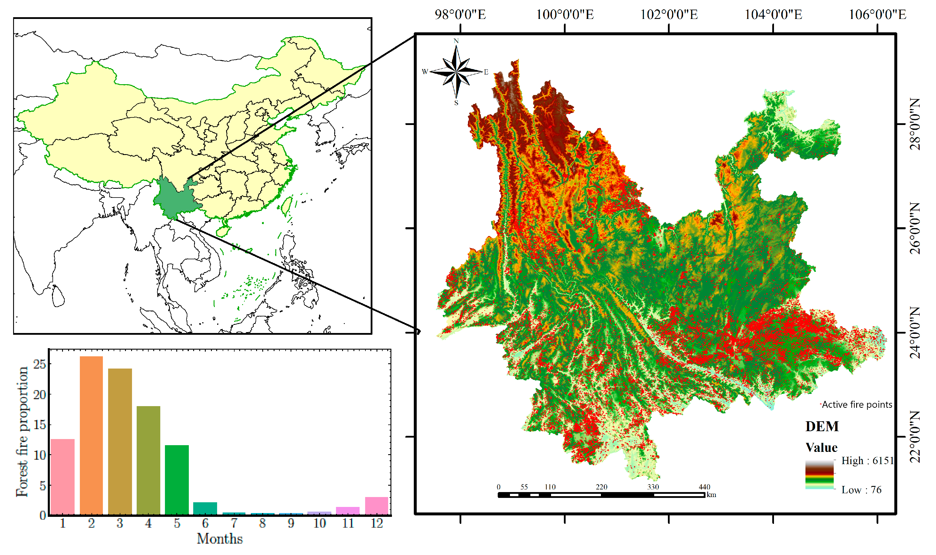
Yunnan Province is located on the southwestern border of China (Figure 1), which is between 21°09′–29° 15′ N and 97° 31′–106°11′ E, with a total area of 394,100 square kilometers. The topography of this region is high in the northwest and low in the southeast and descends step by step from north to south. Mountainous areas account for 88.64% of the total area of this province. Yunnan generally has a subtropical monsoon climate with large daily temperature differences and small annual temperature differences. The temperature varies significantly vertically with the height of the terrain. Precipitation is very unevenly distributed over the seasons [26]. The wet season runs from May to October, accounting for 85% of the total annual rainfall. The dry season runs from November to April. The topography and meteorology of this region are suitable for the growth of forests. By 2020, the forest area of Yunnan Province had reached 24.936 million hectares with 65.04% forest coverage, making it one of the provinces with abundant and diverse forest resources in China [27]. The dominant tree species in Yunnan are Pinus yunnanensis, Pinus armandii, and Keteleeria evelyniana, all of which are flammable tree species [28].
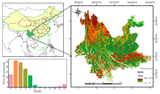
Figure 1.
Study area (map) and locations of forest fire points from NASA’s Fire Information for Resource Management System. The histogram shows the proportion of forest fire points in the study area from 2004 to 2018.
According to the statistics of the Yunnan Forest Fire Brigade, there were 5036 forest fires in Yunnan from 2004 to 2018. It is a region in China with severe fire hazards. Meanwhile, in densely populated forest areas, there has always been the practice of burning wasteland. If the fire is used carelessly in the dry season, it can easily cause large-scale forest fires. As a result of the above factors, the potential risk of forest fires in Yunnan Province is high, and its forest fire prevention work faces serious challenges [29].
2.2. Data Resources
2.2.1. Fire Point Inventory
Fire point data were collected from the NASA Fire Information Resource Management System (FIRMS) Visible Infrared Imaging Radiometer Suite (VIIRS) 375 m anomalous hotspot remote sensing data [30]. The VIIRS sensor provides a spatial resolution of two types of anomalous hotspot data, 750 and 375 m, with global coverage every 12 h. It is widely used in fire point monitoring [31], burned area mapping [32], and fire emission assessments [33]. Compared to a moderate resolution imaging spectroradiometer (MODIS), VIIRS products have higher precision and more significant application potential.
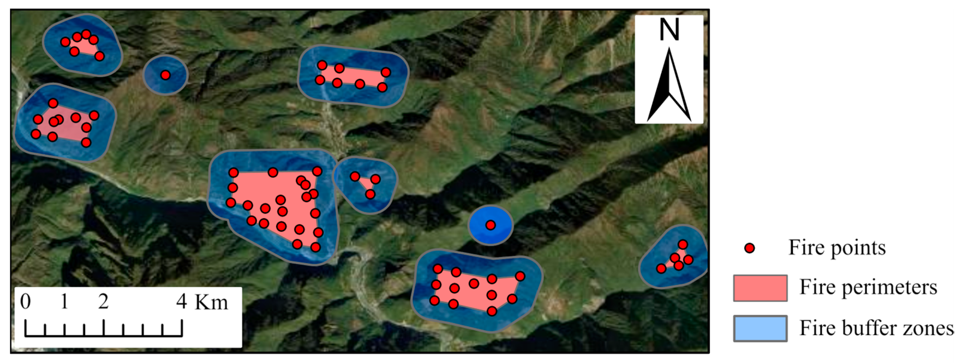
The VIIRS 375 m dataset encompasses critical fire characteristics, including fire point coordinates, ignition dates, and confidence levels. In extracting fire points, VIIRS high-confidence thermal anomaly data (Type H) from Yunnan Province spanning the years 2004 to 2018 were selected to represent forest fire points. To mitigate the influence of stationary heat sources, such as power plants, thermal anomalies not classified as forest land were excluded from the analysis. The resulting dataset still contained a significant number of fire points, attributed to VIIRS’s capability of capturing changes in the perimeters of fire scenes during the spread of fires. To refine the dataset further, we adopted an adaptive k-means clustering algorithm, as referenced in [34], which clusters the thermal anomalies based on longitude, latitude, and occurrence time. The method was employed to identify points belonging to the same fire incident and to construct fire polygons encompassing all points involved in individual fire events. Ultimately, 20,676 fire incidents were identified, as illustrated in Figure 2. Among these, the earliest occurring points were retained as forest fire points for experimental purposes, resulting in a dataset of 70,274 fire points. While these data may still include points related to the same fire incident, variations were present within them. For the sake of expanding the training dataset, these points were not excluded.
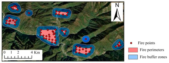
Figure 2.
The portion displaying fire incidents identified through adaptive k-means clustering.
In addition to the fire points, random points were also necessary and selected to serve as nonfire points. For the dependent variable labels, ignition points were labeled as “1” and nonignition points as “0”. To ensure the accuracy of the nonfire point selection, a 500 m buffer zone was established around the fire polygons obtained from clustering, prohibiting the allocation of random points within this buffer on the same day. Furthermore, to maintain data balance and minimize bias, we randomly selected an equal number of nonfire points based on previous research [14,16,17,18,20]. The selection of random points as nonfire points ensured dual randomness in both temporal and spatial dimensions. The dataset, comprising both fire and nonfire points, was divided based on the occurrence dates, with 70% of the data allocated for training and the remaining 30% for testing. To address the issue of data leakage, we ensured that the data for each distinct fire event were exclusively contained within either the training or test set and not both. This approach prevented the overlap of fire events across sets, thereby eliminating the risk of the model being inadvertently exposed to test conditions during training.
2.2.2. Forest Fires Risk Influencing Factors
The occurrence of forest fires is the result of a combination of factors. We classified these factors into four major categories based on previous studies: meteorological factors, topographic factors, vegetation factors, and human activity factors.
The influencing factors related to topography include elevation, slope, and aspect. Usually, the higher the elevation and the higher the moisture content of the vegetation, the lower the risk of forest fires [35]. Slope can affect the rate of fire spread. For uphill fires, combustible materials in the upper part are preheated by the fire below, causing a significant loss of moisture and accelerating fire spread. Also, the greater the slope, the easier it is to lose moisture from the soil, the drier the vegetation tends to be, and the higher the risk of forest fires [36]. Slope aspects can be divided into sunny slopes and shady slopes. Vegetation on sunny slopes is more susceptible to forest fires due to prolonged exposure to sunlight, increased surrounding temperatures, and reduced air humidity [37].
Meteorological factors include temperature, humidity, precipitation, wind speed, and hours of sunshine. The temperature is a crucial factor in forest fire occurrence and spread. The higher the temperature, the stronger the transpiration of vegetation, leading to a decrease in the water content of combustible materials and an increase in the risk of forest fires [38]. The amount of precipitation and the air’s relative humidity affect the vegetation’s water content [39]. In addition, the wind can accelerate airflow, reduce air humidity, and increase the likelihood of forest fires.
The occurrence of forest fires is not only influenced by same-day meteorological factors but also by the cumulative effects of previous climate. One of the most commonly used methods to visualize the impact of this cumulative weather effect’s impact on forest occurrence is the forest fire weather index (FWI). The FWI is based on the time-lag equilibrium water content theory. The individual indices of the FWI are calculated from the temperature, relative humidity, wind speed, and precipitation data observed at solar noon each day [40]. The FWI index includes three combustible moisture codes, which are fine fuel moisture content (FFMC), duff moisture content (DMC), and drought code (DC). FFMC represents the fuel moisture of forest litter fuels under the shade of a forest canopy. It is intended to represent moisture conditions for shaded litter fuels, the equivalent of 16 h time lag, and ranges from 0 to 101. The FFMC value varies with the moisture content of combustible material affected by precipitation, temperature, relative humidity, and wind speed. DMC represents fuel moisture of decomposed organic material underneath the litter and represents moisture conditions for the equivalent of 15-day (or 360 h) time-lag fuels. DC represents drying deep into the soil and approximates moisture conditions for the equivalent of 53-day (1272 h) time-lag fuels. It is unitless and has a maximum value of 1000. Extreme drought conditions have produced DC values near 800 [41]. The FFMC, DMC, and DC indicators are a continuous calculation process, and the results of the next day depend on the values of the previous day, so the initial values of the three indicators need to be set. The initial value of FFMC is 85, DMC is 6, and DC is 15 [42].
Vegetation factors include the vegetation normalized index (NDVI) and vegetation type (VT). NDVI is remote sensing data reflecting vegetation’s spatial distribution and density, and it is often used to estimate the vegetation’s growth status and density [43]. The occurrence of forest fires is intricately linked to the type of vegetation as it directly influences the characteristics and quantity of combustible materials.
According to relevant statistics, the vast majority of forest fires that have occurred in recent years have been caused by human activities [44,45]. Ritual fires, spring burning, and wild smoking are the leading causes of human-induced forest fires [46]. We chose population density distribution and distance to roads to characterize the impact of human activities on forest fires. For ease of description, we categorize the distance to rivers as part of human activities. Areas with rivers tend to have moist soil and higher plant moisture content, making them less prone to wildfires. Additionally, rivers can effectively act as barriers to prevent the spread of wildfires [47].
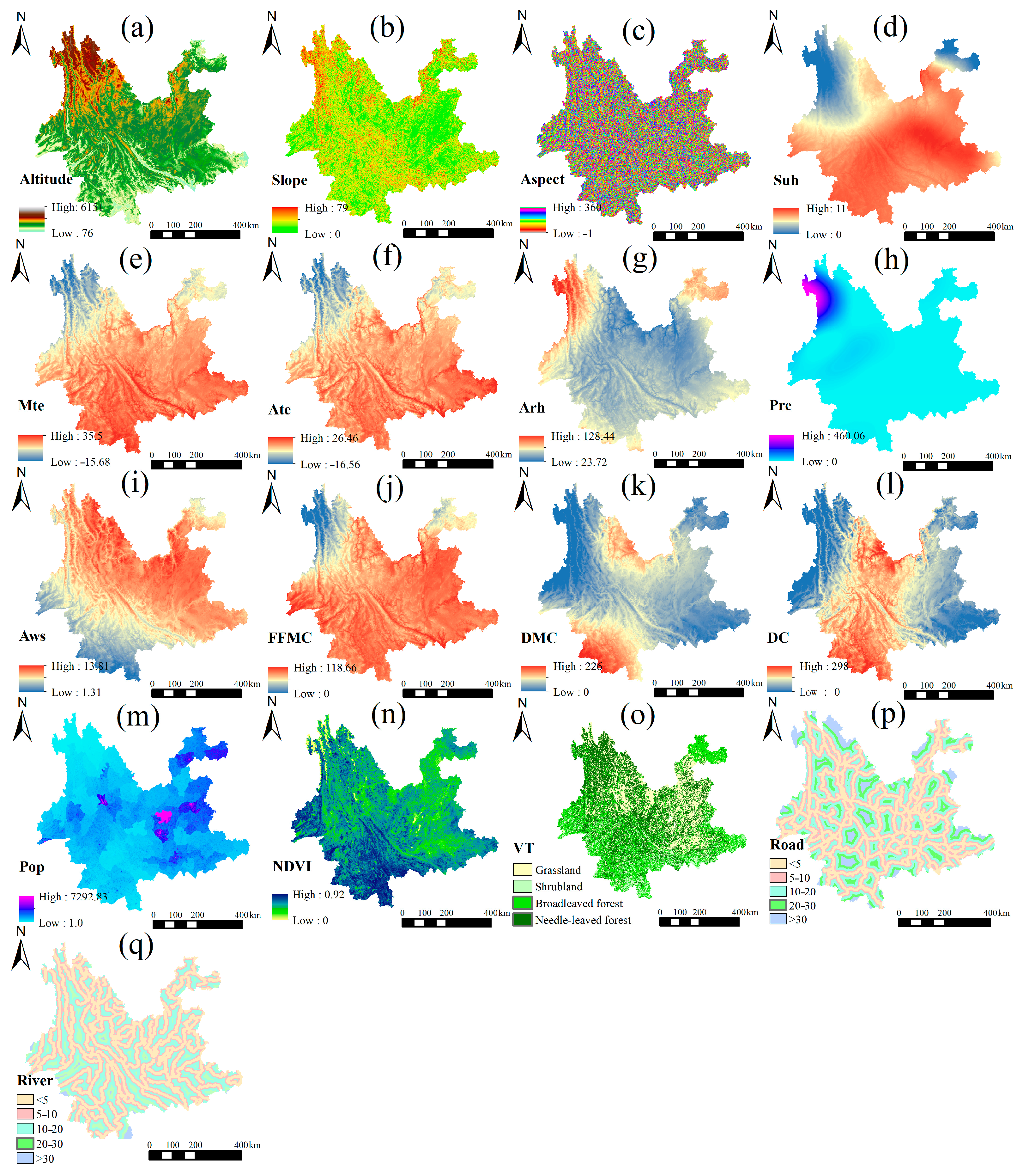
Through the investigation of forest fire risk influencing factors, we finally selected 17 factors as features, and the detailed data description is shown in Table 1. The distribution of influencing factors is shown in Figure 3 (6 March 2018).

Table 1.
Data description of forest fire risk influencing factors.

Figure 3.
Forest fire influencing factors in Yunnan Province: (a) altitude, (b) slope, (c) aspect, (d) hours of sunshine, (e) maximum daily air temperature, (f) average daily air temperature, (g) average daily relative humidity, (h) 24 h cumulative precipitation, (i) maximum daily wind speed, (j) fine fuel moisture content, (k) duff moisture content, (l) drought code, (m) population rate, (n) NDVI, (o) vegetation type, (p) distance to roads, and (q) distance to rivers.
2.2.3. Spatial Interpolation of Meteorological Data
The distribution of meteorological stations in Yunnan Province is characterized by discrete limitations and uneven coverage, necessitating the use of spatial interpolation techniques to derive accurate meteorological data. Spatial interpolation involves mathematically deriving data for unknown regions based on known discrete data and is commonly accomplished through methods such as inverse distance weighting (IDW), kriging, and spline [48]. Studies indicate that, particularly in Yunnan, thin-plate spline interpolation using the Anusplin software yields higher overall accuracy compared to IDW and kriging [49].
Meteorological data were sourced from the “Daily meteorological dataset of basic meteorological elements of China National Surface Weather Station (V3.0)” provided by the China Meteorological Data Network, covering 15 years from 2004 to 2018. To ensure precise interpolation, we selected the three-variable thin-plate spline function with elevation as a covariate, specifically the TVPTPS3 model, based on prior research findings [50]. Utilizing Anusplin software with this model configuration, we generated a spatial interpolation raster dataset for meteorological variables at a resolution of 500 m × 500 m. Precipitation interpolation employed square root transformation due to data range and high uncertainty.
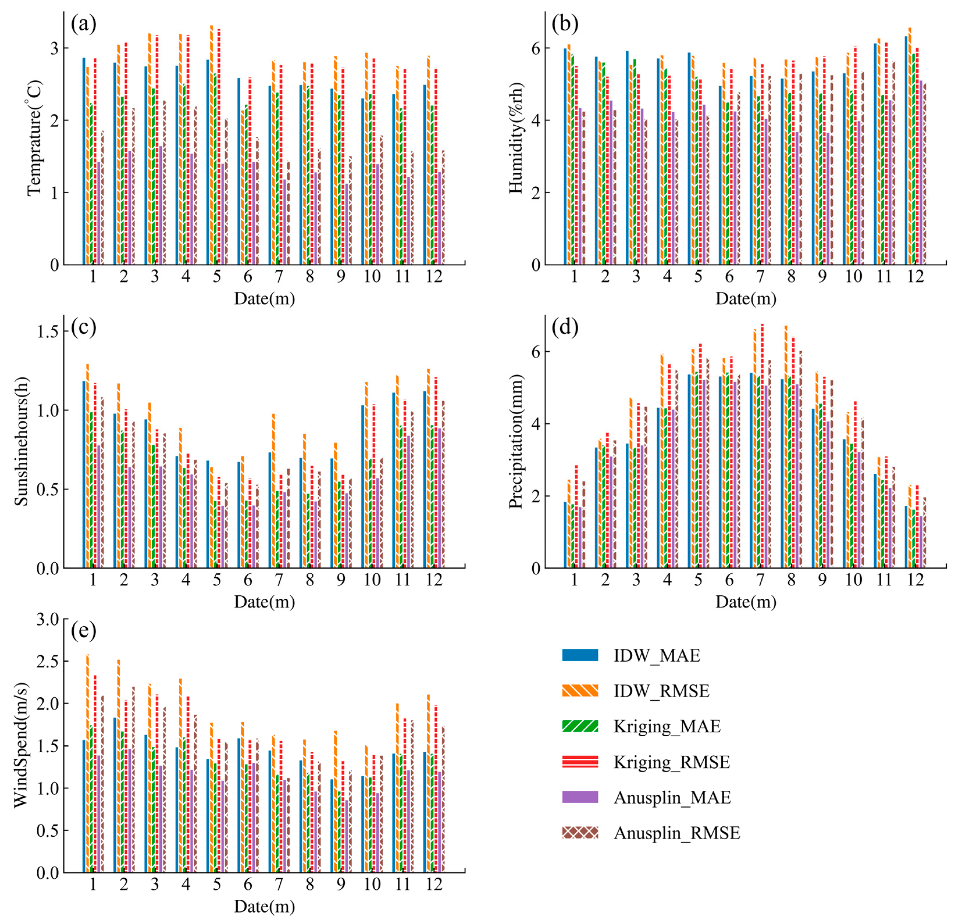
To assess the reliability and applicability of Anusplin interpolation for meteorological feature data, we conducted a comparative analysis with commonly employed kriging [17] and IDW [51] interpolation methods frequently utilized in forest fire prediction or risk assessment. Monthly average meteorological elements from the 15th day of each month (temperature, humidity, precipitation, hours of sunshine, and wind speed) were selected for interpolation processing. Of the 86 meteorological stations, data from 80% (69 stations) were used for interpolation computation, while data from the remaining 20% (17 stations) were used for verification. Mean absolute error (MAE) and root mean square error (RMSE) comparisons between actual and predicted values at verification stations were performed to assess interpolation accuracy [48]. The MAE indicates the level of overall error, while the RMSE reflects the sensitivity and extreme conditions of the sample data estimation. The smaller the MAE and RMSE values, the higher the precision and robustness of the spatial interpolation.
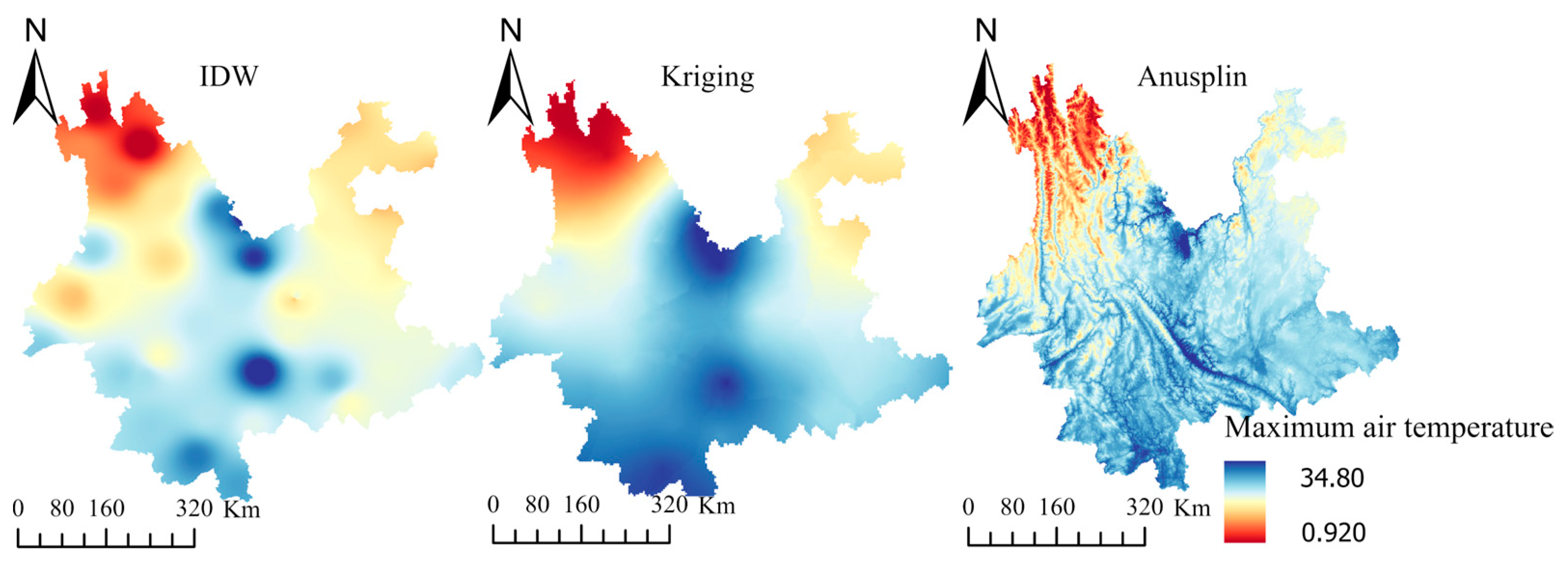
Comparative analysis of IDW, kriging, and Anusplin for average maximum air temperature distribution on 15 May from 2004 to 2018 (Figure 4) revealed distinctive features. The IDW method resulted in locally low- or high-temperature phenomena because it only considered the spatial distance between meteorological stations and points to be interpolated. The kriging method used semivariogram to describe spatial correlation between sites, capturing trends in geographical space using covariance functions. Although it yielded the smoothest interpolation distribution among the three methods, it did not precisely reflect the influence of geographic elements on temperature. The Anusplin method using a regression model based on altitude distinctively delineated mountainous features of the Yunnan region.
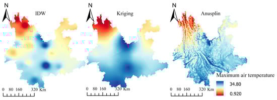
Figure 4.
Distribution of average maximum temperature on 15 May from 2004 to 2018 by IDW, kriging, and Anusplin.
Numerically, a comparison of the verification of the three interpolation methods for average maximum temperature (a), relative humidity (b), hours of sunshine (c), precipitation (d), and wind speed (e) are illustrated in Figure 5, depicting the average MAE and RMSE across each month from 2004 to 2018.
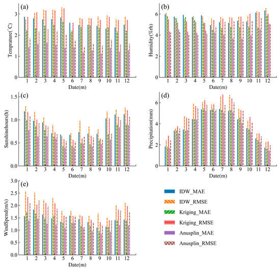
Figure 5.
The average MEA and RMSE for the average maximum temperature (a), relative humidity (b), hours of sunshine (c), precipitation (d), and wind speed (e) across each month from 2004 to 2018 employing three interpolation methods.
Overall, the Anusplin interpolation method achieved the smallest RMSE and MAE values among all the five meteorological elements. As a result, it stood out as the optimal spatial interpolation method for daily basic elements in the Yunnan area, proving that the interpolated data are highly reliable [49].
2.2.4. Data Preprocessing
To reduce implicit transformations in the model and eliminate outliers in raw data to improve accuracy, data preprocessing is the first crucial step in machine learning. We extracted forest fire influencing factors as features from raster data using the ArcGIS software and converted them to tabular data. Among the features, aspect, VT, road, and river were categorical variables, while the rest were continuous variables. We chose the z-score normalization method to transform continuous variables into a form with a mean of 0 and a standard deviation of 1 [52]. The formula is as follows:
where is the normalized data, is the original data, and are the mean and standard of the full original data, respectively.
2.3. Methodology
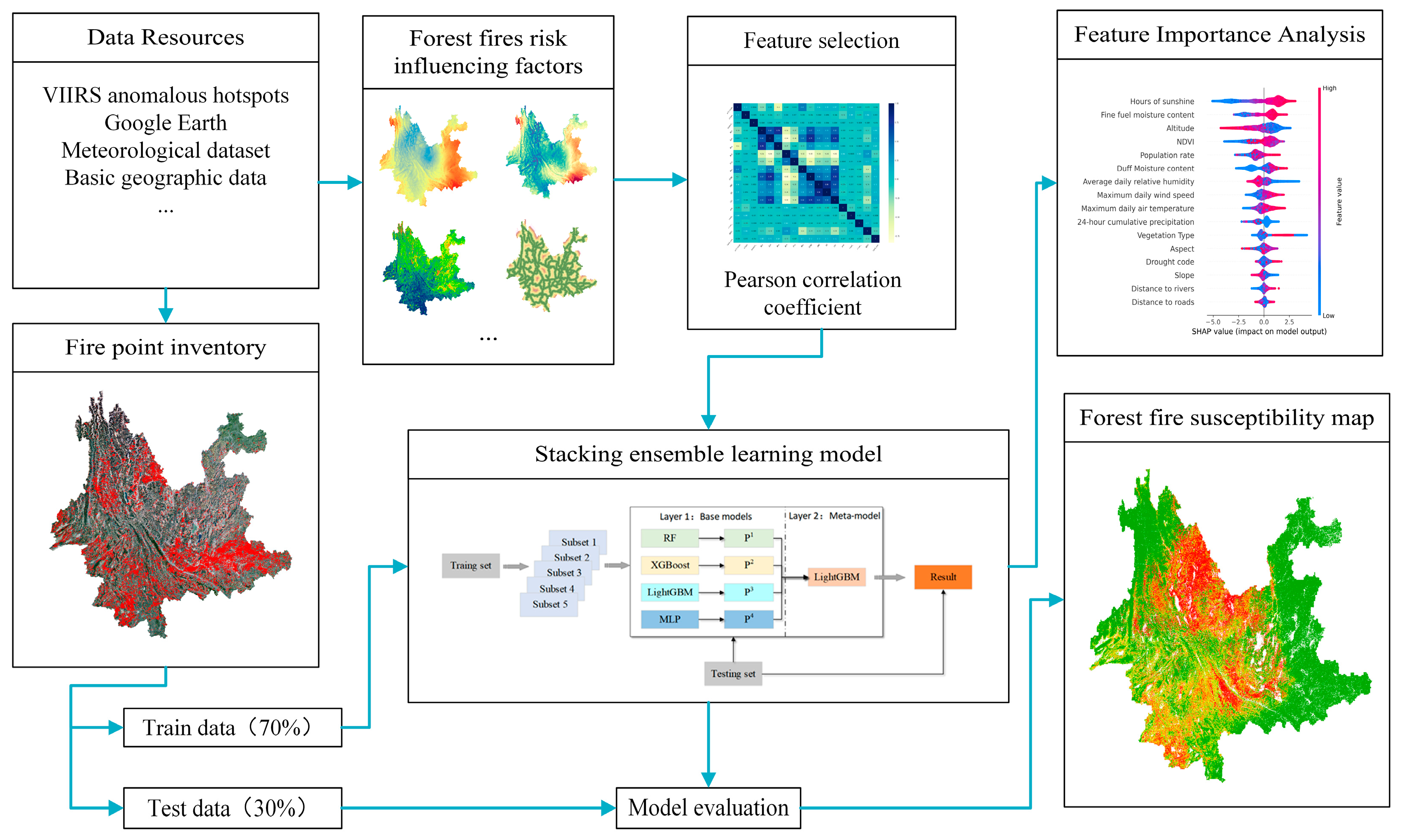
The methodology included five steps: (1) selecting the forest fire influencing factors, (2) modeling the forest fire risk using the stacking ensemble technique, (3) ranking feature importance based on the SHAP interpretation framework, (4) evaluating the forest fire risk prediction models, and (5) producing and validating the forest fire susceptibility maps. Figure 6 shows the flowchart.

Figure 6.
Flowchart of the methodology.
2.3.1. Selecting the Forest Fire Influencing Factors
Feature selection is usually required before modeling, which can prevent inaccurate model prediction due to multicollinearity among features. We used the Pearson correlation coefficient [53], tolerance level (TOL), and variance inflation factor (VIF) to identify feature variables with high covariance. Pearson correlation coefficient >0.8, tolerance (TOL) <0.1, and variance inflation factor (VIF) >10 are usually considered signs of multicollinearity [54]. The features that did not satisfy the above conditions were not used to construct the model.
2.3.2. Modeling the Forest Fire Risk Using the Stacking Ensemble Technique
Single machine learning models usually have various drawbacks. Ensemble learning involves combining individual models together to form a model with stronger generalization performance, effectively reducing or eliminating the limitations of individual machine learning models.
Stacking is a heterogeneous ensemble learning model [55]. The heterogeneous ensemble refers to forming a strong classifier by combining several classifiers with different principles to enhance the generalization ability [56]. The pseudo-code of the Stacking algorithm such as Algorithm 1.
| Algorithm 1: Stacking fusion model. | |
| Input: Four models in the first layer: { = RF, = XGBoost, = LightGBM, = MLP} = LightGBM} | |
| Output: The prediction results on the testing data. | |
| //Training the first layer model | |
| 1: | : |
| 2: | ; |
| 3: | ://k-fold cross validation |
| 4: | ; |
| 5: | ); |
| 6: | ); |
| 7: | ; |
| 8: | End For |
| 9: | End For |
| //Training the second layer model | |
| 10: | ; |
| 11: | according to the row to get the testing data of second layer: ; |
| 12: | ; |
| 13: | ; |
Figure 7 shows the structure of the proposed stacking fusion model, which contains two layers. The first layer contains several base models, while the second has only one metamodel. In order to avoid the problem of poor generalization ability due to the small scale of data division, base models are usually trained by cross-validation. The results of numerous training of base models in the first layer were used as the new training and testing sets, and the metamodel in the second layer was trained and predicted using the new training and testing sets. The following pseudo-codes describe the procession of the model method in detail.
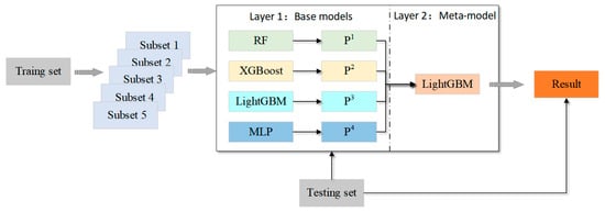
Figure 7.
The structure of the stacking fusion model.
The structure of the stacking fusion model is based on the prediction ability and variance of the base model, so the model with strong prediction ability and high diversity should be selected as the base model in the first layer of the stacking model. For the second layer, the metamodel should have a strong generalization ability to find and correct the bias of multiple base models for the training set. Hence, we used four heterogeneous machine learning algorithms (random forest, XGBoost, LightGBM, and MLP) as the base model and LightGBM as the metamodel. These four base models are briefly described below.
Random forest (RF) is an ensemble learning model design based on the bagging framework [57]. Random forest integrates decision trees as the base estimators and introduces sample random sampling and feature random sampling in the training process. Random forest significantly improves the accuracy and stability of the model, reduces sensitivity to noise and outliers, and effectively avoids overfitting.
eXtreme gradient boosting (XGBoost) is a novel gradient boosting decision tree (GBDT) model [58]. Unlike RF, GBDT is an ensemble learning model based on the boosting framework. Each estimator of GBDT relies on the residuals formed by the previous round of estimator training for the current round. The final result is obtained by accumulating all the results, which is serially generated. In contrast, RF’s base estimators are generated in parallel, and the final results are obtained by majority voting. The XGBoost uses Taylor’s second-order expansion to optimize the loss function, which reduces the training time compared to GBDT and thus improves the efficiency of the solution. It also incorporates a regular term to reduce model complexity and prevent overfitting. The core of XGBoost is to build new trees by continuously splitting features to fit the residuals between the last prediction and the actual value and to sum up the results of all trees as the final prediction result.
The light gradient boosting machine (LightGBM) introduces a leaf-wise leaf growth strategy with a depth limit, a histogram algorithm, a gradient-based one-sided sampling (GOSS) algorithm, and an exclusive feature bundling (EFB) algorithm based on the traditional gradient boosting tree [59]. All four algorithms ensure that the model accuracy is not affected and improve the model training speed under the growth of sample data volume and feature volume.
Multilayer perceptron (MLP), also called artificial neural network (ANN), mainly consists of three parts: input layer, hidden layer, and output layer [60]. The layers of MLP transform the output through the activation function, which can handle complex multi-input and multioutput nonlinear problems and is very good for classification problems.
The base model of stacking determines the optimal hyperparameters by Bayesian optimization [61]. We used accuracy (ACC) as the evaluation indicator for each prediction effectiveness and combined it with a five-fold cross-validation approach by comparing the prediction effectiveness in the test set.
The experiments were conducted on a computer with an Intel i7-12700H processor and 16 GB memory, and the operating environment was a 64-bit Windows 11 system. The Scikit-learn tool library in Python 3.8 was used for model construction, and the bayes_opt tool library was used for Bayesian optimization. The optimal set of hyperparameters for each model is shown in Table 2.
Table 2.
The optimal set of hyperparameters for each model.
2.3.3. Ranking Feature Importance Based on SHAP Interpretation Framework
Feature importance is a method for scoring the input features of a prediction model, which can reveal the relative importance of each feature. The Scikit-learn tool library provides the internal method for tree models such as RF, XGBoot, and LightGBM to return feature importance. However, this method is usually based on the training set, and the relative importance of feature variables may not be accurate when the model is overfitted. As for machine learning algorithms, such as neural networks, which are not based on tree models, feature importance is not available.
The stacking model proposed in this study has a complex internal structure. It is difficult to determine the correlation between the input and output, so the feature importance cannot be obtained using the internal mechanism of the model. We used the SHapley Additive exPlanation (SHAP) interpretation framework to obtain the Shapley value of each feature to indicate the feature’s importance. The SHAP is an additive feature attribution model based on the cooperative game theory [62]. The SHAP value can be used to represent each feature’s marginal contribution value and measure the feature’s importance [63]. The SHAP value of feature j is defined as follows:
where N represents the set of all features, and S represents all feature subsets obtained from F after removing the feature j. represents the output of the machine learning model of the feature subset S. represents the cumulative contribution value of feature j.
2.3.4. Evaluating the Forest Fire Risk Prediction Models
As explained in the previous section, forest fire risk prediction is a binary classification problem, so the threshold value needs to be set when predicting whether a sample belongs to a fire point. In the case of a balanced number of positive and negative samples, the threshold value can be set to 0.5. When the calculated probability is greater than 0.5, the sample is judged to be a fire point and vice versa for a nonfire point.
We used the confusion matrix and its associated parameters to verify the predictive performance of different models. The confusion matrix contains four possible outcomes: true positive (TP), true negative (TN), false positive (FP), and false negative (FN). TP and TN denote the number of correctly classified fire point and nonfire point samples, respectively, while FN and FP denote the number of misclassified fire point and nonfire point samples, respectively.
The receiver operating characteristic curve (ROC) is a valuable tool for evaluating the performance of forest fire risk prediction models [64]. The area under the curve (AUC) can quantitatively reflect the model performance measured on the basis of the ROC with values between 0.5 and 1. The closer the AUC to 1, the more accurate the model.
In addition to the above classification performance indicators, accuracy, precision, recall, and F1 score were used to evaluate the model effect [65]. The higher accuracy, precision, recall, and F1 score represent the better predictive ability of the model.
2.3.5. Producing and Validating the Forest Fire Susceptibility Maps
In general, the model evaluation indicators, as described above, should be sufficient to validate the predictive capability of the models. However, susceptibility mapping for forest fire risk prediction is critical because it provides preliminary information on which areas are at risk [13]. Therefore, each model must be output as a susceptibility map to validate and evaluate performance.
The forest fire susceptibility map is a probability map of fire occurrence, indicating the probability of forest fire risk. The trained model was applied to the entire study area, and the probability of forest fire occurrence was calculated for each cell. The equal intervals method was used to reclassify susceptibility into five classes, including extremely low (0~0.2), low (0.2~0.4), medium (0.4~0.6), high (0.6~0.8), and extremely high (0.8~1).
A good forest fire susceptibility map should contain more fire points with fewer high susceptibility areas. For this purpose, we introduced fire density (FD) as a new evaluation indicator. FD is defined as the ratio between the proportion of fire points falling into each class and the proportion of the number of pixels in that class. The higher the FD for a given class, the more fire points per unit area for that class. The formula for FD is as follows:
where represents the number of fire points falling in class i, represents the total number of fire points in the study area, represents the number of cells in class i, and represents the total number of cells in the study area.
3. Results
3.1. Forest Fire Influencing Factor Selection
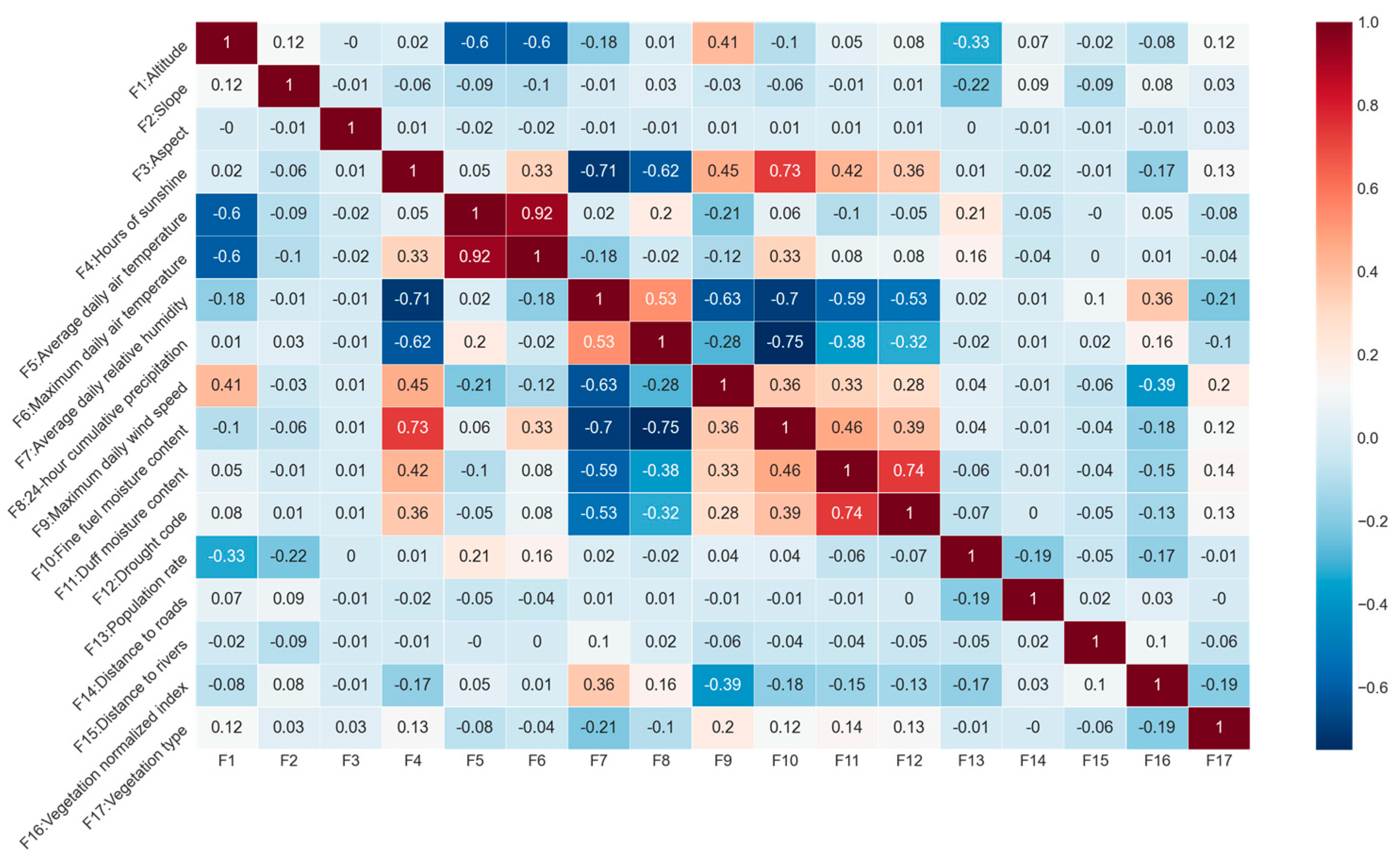
Figure 8 illustrates the Pearson correlation coefficients among the 17 features. The correlation analysis indicated that, with the exception of the strong correlation between average daily air temperature and maximum daily air temperature (0.92), most factors exhibited weak correlations with each other. In light of practical considerations and the understanding that elevated temperatures are a crucial component of conditions conducive to forest fire risk, average daily air temperature was subsequently excluded from the features.

Figure 8.
Pearson correlation coefficient results.
The multicollinearity analysis showed the tolerances (TOL) and variance inflation factors (VIF) of the remaining 16 features, as presented in Table 3. The TOL of the features ranged from 0.20 to 0.92, and the VIF ranged from 1.09 to 5.0, which satisfied the threshold requirements of TOL >0.1 and VIF <10. This indicated that there was no multicollinearity among the selected features, and it could be used for model training and validation.
Table 3.
Multicollinearity diagnosis results of features.
3.2. Model Comparison and Validation
The stacking fusion model was compared with its four base models. We used the six evaluation indicators in Section 2.3.4 to validate the models’ prediction effectiveness and generalization ability.
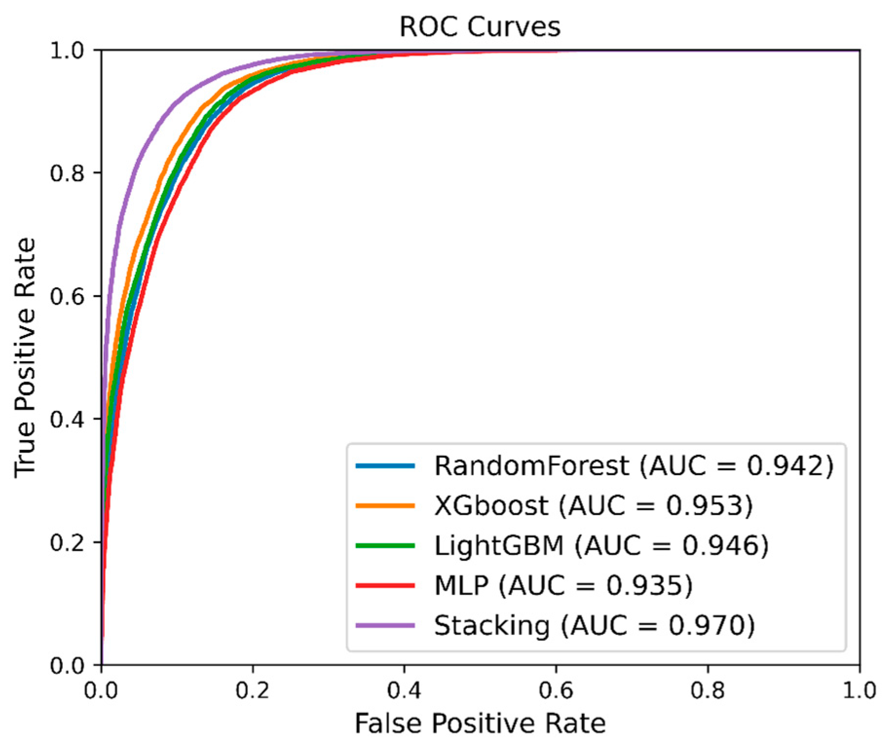
Figure 9 shows the ROC curve of the five models in the testing dataset. The results showed that the stacking fusion model had the highest AUC value (0.9701), followed by XGBoost (0.953), LightGBM (0.946), RF (0.942), and MLP (0.934). As demonstrated in Table 4, the stacking fusion model was better than the other four models in terms of accuracy, precision, recall, and F1 score. The proposed stacking fusion model, compared to the best-performing model among the single models, XGBoost, improved by 2.24% in accuracy, 2.22% in precision, 2.24% in recall, and 2.12% in F1 score.

Figure 9.
ROC curves and AUC results.
Table 4.
Performance of different prediction models.
The predictive power of all five models in this study was within the acceptable range, but the stacking model had better generalization ability and better prediction accuracy.
3.3. Forest Fire Susceptibility Map
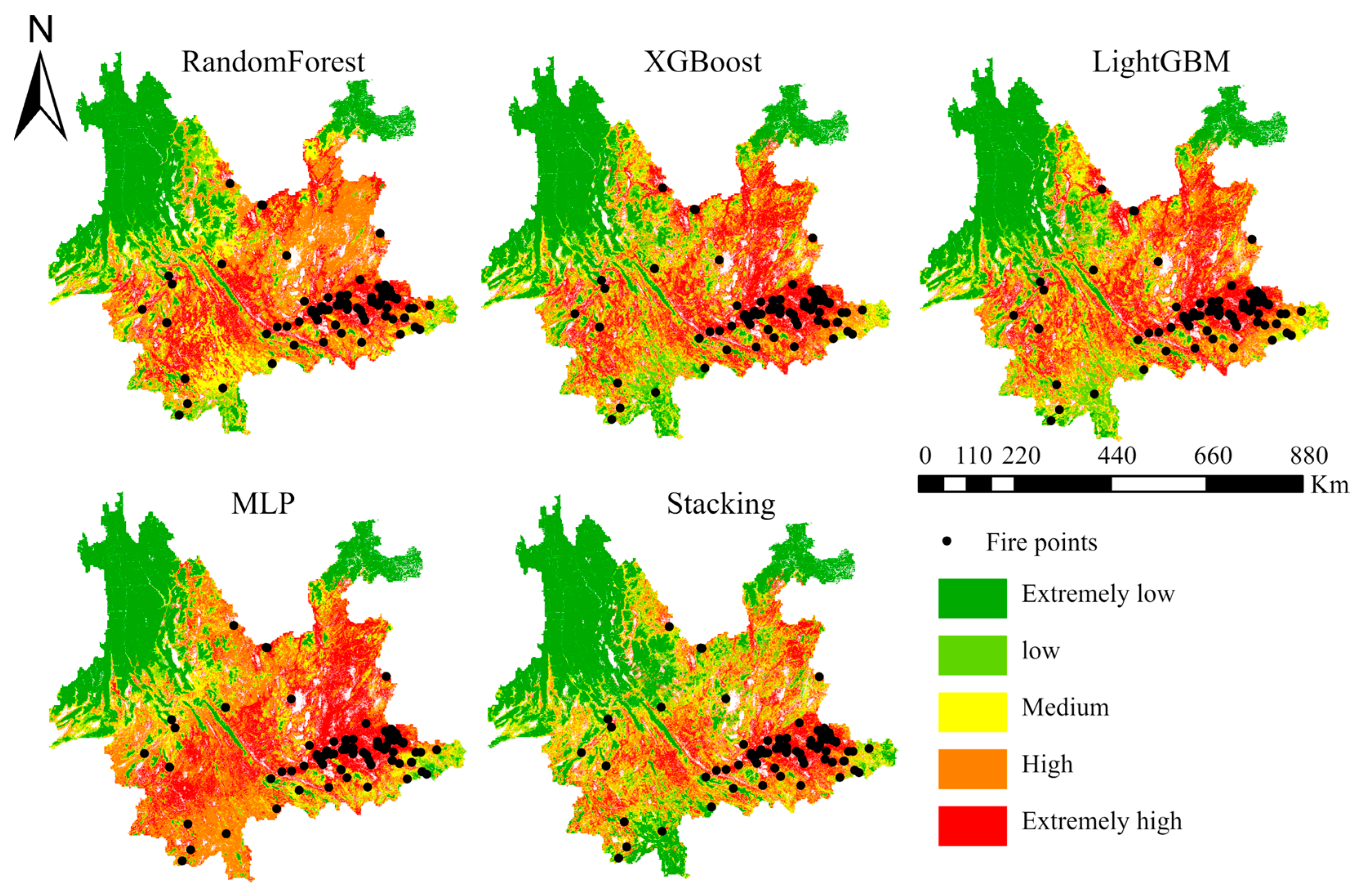
To comprehensively compare the performance of the five machine learning models and present their prediction outcomes more clearly, we conducted an analysis and comparison of the forest fire susceptibility maps generated by these models. The months of February and March are recognized as peak periods for forest fires in Yunnan Province. For the validation of the predictive capabilities of the five models, we selected the complete datasets for February and March in the year 2018. Notably, the fire point data for these months were deliberately excluded from the training dataset. We randomly selected 6 March 2018 from the two peak months and utilized five models to generate forest fire susceptibility maps for that specific day. The resolution of these maps was set at 500 m, as depicted in Figure 10.

Figure 10.
Forest fire susceptibility maps and observed fire points distribution on 6 March 2018.
Overall, the five maps had similarities in spatial distribution. For example, the extremely high susceptibility area was mostly distributed in the eastern region, and most fire points also fell in the extremely high class. In addition, there were some differences among the five maps. The MLP had the largest number of extremely high and high susceptibility areas.
For quantitative susceptibility map analysis, we employed fire density (FD) to assess the reliability and accuracy of the results. A higher FD value in a specific area indicates a greater number of fire points per unit area in that region. Table 5 illustrates the FD values corresponding to the susceptibility maps for the five models across different susceptibility levels, ranging from extremely low to extremely high. The distribution aligns well with the actual scenario, wherein fire points are more likely to occur in extremely high susceptibility areas while the probability is considerably lower in extremely low susceptibility areas. At the same time, the stacking fusion model exhibited a significantly higher FD value in the extremely high susceptibility area (2.68) compared to other models. This suggests that the stacking fusion model excels in accurately identifying fire points with only a minimal number of misclassifications in low susceptibility areas.
Table 5.
The evaluation of forest fire susceptibility classes.
3.4. Feature Importance
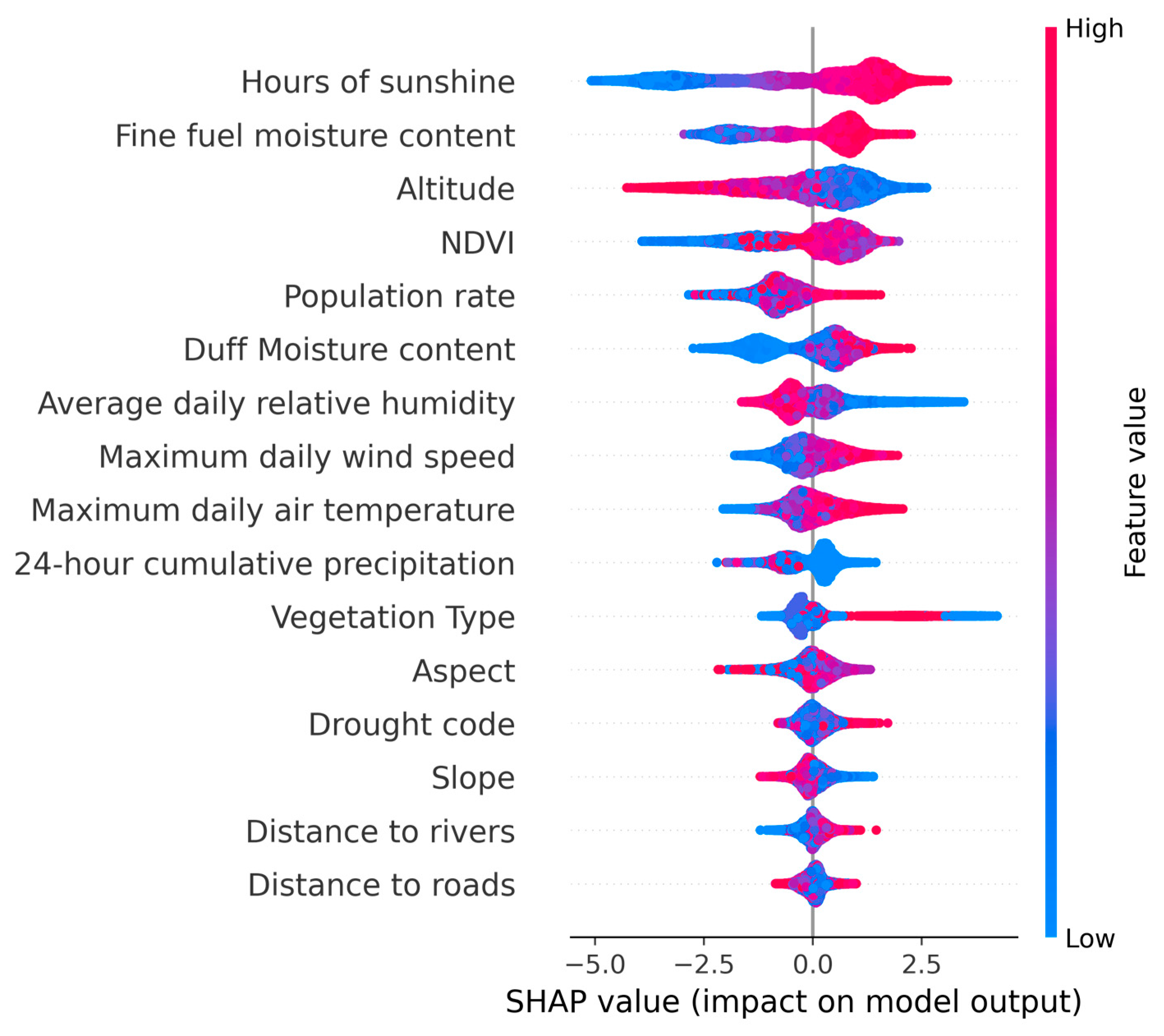
The predictions of the stacking fusion model were analyzed using SHAP to generate a comprehensive feature summary plot illustrating feature importance and effects. In Figure 11, each row corresponds to a feature, with features arranged in descending order of importance (from top to bottom). Each point represents the SHAP value of an instance, and the color gradient from blue to red indicates the feature’s low to high value. The x-axis represents the SHAP values, where a positive value signifies a positive effect on the model output and a negative value indicates a negative effect on the model output.
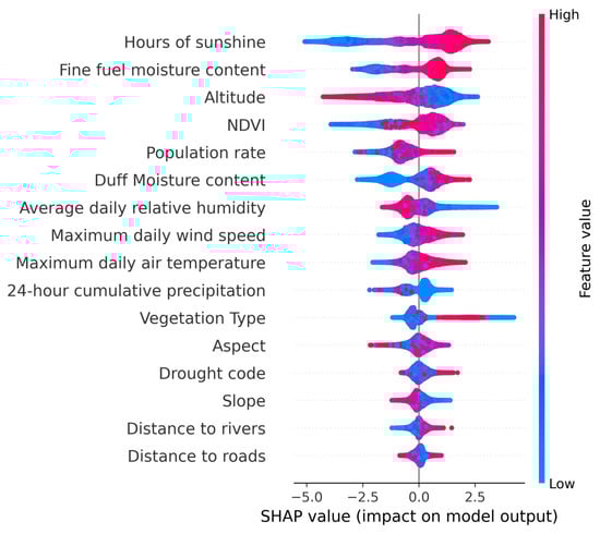
Figure 11.
SHAP summary plot for the stacking fusion model.
As shown in Figure 8, features such as sunshine duration (Suh), altitude, fine fuel moisture code (FFMC), normalized difference vegetation index (NDVI), duff moisture code (DMC), population density (Pop), average relative humidity (Arh), maximum daily air temperature (Mte), maximum daily wind speed (Mws), 24 h cumulative precipitation (Pre), and vegetation type (VT) significantly influenced the model’s predictive output. Specifically, an increase in the values of Suh, FFMC, NDVI, DMC, Pop, Mte, and Mws resulted in higher SHAP values, indicating a positive impact on the occurrence of forest fires. Conversely, altitude, Arh, and Pre exhibited a negative influence on the predicted output as their values increased. For categorical features, such as aspect, slope, and VT, where the feature values represent categories, it is challenging to assess their impact on the model output based solely on value changes. However, their clustered distribution suggests that specific categories had a significant impact on the model.
4. Discussion
4.1. Predictive Model Comparison
Forest fire risk prediction is affected by different meteorological, topographical, and human factors in the study area, which is complex and varied. Thus, it is difficult to have a general model to solve the prediction problem in all areas [66].
We opted for four models, namely, random forest (RF), XGBoost, LightGBM, and multilayer perceptron (MLP), each exhibiting robust generalization capabilities and significant theoretical differences, as our base models. Leveraging the stacking ensemble learning technique, we constructed a multimodel fusion model by combining them. When the stacking model was compared with these four base models, experimental results showed that the stacking fusion model improved the prediction performance (highest AUC values and accuracy). This improved effect resulted from reducing the bias and variance and avoiding overfitting problems [67]. Among the four base models, tree-based models, namely, RF, XGBoost, and LightGBM, demonstrated comparable performance in accuracy, precision, recall, F1 score, and AUC evaluation metrics. They outperformed MLP, confirming the notion that neural networks may not perform as well as tree models, such as random forest and XGBoost, on tabular data [68].
When modeling the forest fire susceptibility map, MLP, in order to fit the sample data, predicted the forest fire risk for the entire Yunnan Province as a higher level, failing to reflect the polar distribution of extremely high and extremely low forest fire risks. However, some argue that an extreme polar distribution of very high and very low risks may not be the optimal choice for susceptibility maps as moderate risk levels also provide crucial information [51]. The stacking model proposed in this study leverages the advantages of integrating multiple models, allowing it to encompass the maximum number of extremely high susceptibility areas with minimal coverage, achieving the highest fire density without losing the intermediate risk levels. We believe it strikes a good balance between these two perspectives.
There is no free lunch, and no one model is always good [69]. The stacking fusion model achieves the highest accuracy, but it also has the most complex structure, requiring a considerable amount of time for training and incurring high costs. Given these considerations, many commercial companies may opt for a single model, such as XGBoost or LightGBM. In the realm of model selection, balancing accuracy and complexity has always been a focal point in machine learning research. Additionally, compared to other tree-based models, stacking cannot identify the relative weights of features, leading to lower interpretability. To address this, incorporating Shapley values on the foundation of the SHAP interpretability framework enhances the interpretability of the stacking model.
4.2. Impact Factor Analysis
Meteorology was most closely related to forest fire risk. As shown in Figure 11, the first two features were both meteorological factors. Forest fires in Yunnan Province mainly occur in the dry season (January–May). According to Figure 11, moderate correlations were observed among specific factors, such as sunshine duration and precipitation as well as sunshine duration and relative humidity. This suggests that many variables exhibit interdependence. The dry season is characterized by abundant sunlight, low precipitation, gradual temperature increase, low air humidity, and the impact of subtropical monsoons. These conditions contribute to a continuous decrease in the water content of combustible materials, making the area more susceptible to forest fires.
Regarding vegetation factors, some studies suggest that higher NDVI values indicate a higher frequency of forest fires. As shown in Figure 11, the feature values of NDVI were positively correlated with SHAP values, confirming this observation. Additionally, we observed a clustered distribution of vegetation types, as shown in Figure 11. Upon examining the vegetation types corresponding to these high SHAP values, we found that they were predominantly coniferous forests, such as pine trees. This indicates that different vegetation types can also influence the occurrence of forest fires [70].
As for topographic factors, altitude significantly impacted the model output, probably because of the significant variations in altitude in Yunnan. Areas with high elevation have low temperatures, and together with the lack of human presence, the probability of forest fire risk is low. Aspect had less influence on the model output, probably because Yunnan is located at low latitudes and the difference in heat between shaded and sunny slopes is insignificant.
On the human activity factors, the SHAP framework had a poor interpretation of Pop, and many points with high feature values were mixed with those with low feature values. It may be that, within a certain threshold, an increase in population density would indicate high human activity in the forest, increasing forest fire frequency [71]. However, forest fires are less likely to occur in towns with high population density, where forest cover is low. In general, the distance from rivers and roads is considered a crucial feature for assessing forest fire risk. However, in this study, these two features were found to have a weaker impact, possibly related to the categorization of distance. In studies involving large-scale regions like Yunnan Province, the data used lacked information on roads below the county level, making it challenging to categorize road distances in units as small as meters, as is carried out in smaller-scale studies [72]. This categorization might not have fully explored the correlation between fire occurrences and road distance, leading to a relatively weak influence on the model output.
Based on the analysis above, in Yunnan Province, with its varied topography and rich biodiversity, managing forest fires is challenging. Advanced monitoring through satellites and drones is crucial for early fire detection, especially in remote areas. This should be coupled with a rapid response system combining aerial and ground teams for effective fire suppression. The province’s rugged terrain requires special firefighting methods and equipment, particularly for mountainous regions. Helicopters are vital for surveillance and fighting fires in hard-to-reach areas [20]. Additionally, managing vegetation and firebreaks is essential to reduce fuel and prevent wildfire spread. The distinct dry and wet seasons in Yunnan also demand an adaptive management strategy to effectively prevent and control fires and to mitigate their impact.
4.3. Limitations and Prospects
The quality of the input data is critical. Both the type and resolution of data can have an impact on model construction. Different versions of elevation, vegetation, and meteorological data may lead to different forest fire risk prediction results. Although some free elevation data are currently available [73], unfortunately, there are still difficulties in obtaining high-resolution meteorological data and vegetation data. As more and more high-resolution data become available, the reliability of predictive assessment modeling developed based on machine learning will continue to increase in the future.
In constructing our dataset, we aimed for a balanced representation and minimized bias by setting a fire to nonfire point ratio at 1:1, aligning with prior research insights. However, due to the infrequency of forest fires, this sampling approach may potentially overemphasize the proportion of fire incidents, leading to inadequate model training and reduced accuracy. Recent work in landslide susceptibility assessment [74] suggests the use of Bayesian optimization algorithms to optimize sample ratios, resulting in improved AUC values. Given the rarity of forest fires, similar to landslides, our future research will explore the applicability of Bayesian optimization algorithms in determining the optimal ratio of fire and nonfire points.
The proposed stacking fusion model in this study effectively enhances prediction accuracy and addresses the challenge of selecting the appropriate machine learning algorithm. Nonetheless, a notable drawback is the model’s increased complexity and reduced interpretability compared to other models. Investigating the integration of interpretable machine learning models in forest fire risk prediction, elucidating corresponding trends in the feature space, and explaining the decision process for specific cases pose challenges for future research.
Although our current model primarily leverages static spatiotemporal influencing factors, we acknowledge the growing body of research utilizing neural network models based on time-series data to enhance predictive capabilities [75]. Recognizing the potential advancements offered by incorporating temporal dynamics, our future research will explore the integration of time-series data into the modeling framework. This evolution aims to capture the dynamic nature of forest fire risk, providing a more nuanced and accurate predictive assessment. As temporal data availability and computational capabilities advance, this avenue holds promise for refining and advancing our predictive modeling strategies.
Considering the ultimate goal of applying the model to the entire Yunnan Province, future efforts will focus on validating and adjusting the model to ensure its applicability and reliability across the entire domain. This step is critical as the reported metrics, while encouraging, may not fully reflect the model’s performance when applied to the broader and more diverse dataset of the entire province.
5. Conclusions
Forest fire management is a protracted undertaking necessitating the development of reliable fire risk prediction models tailored to local conditions. The key contributions of this study are as follows:
- We devised a stacking fusion model by amalgamating four disparate machine learning methods (RF, XGBoost, LightGBM, and MLP) for forest fire risk prediction. Although currently limited by the specific sampling dataset used in this study, the model showed promising results in generating daily forest fire sensitivity maps.
- Through multiple covariance tests and Pearson coefficient analyses involving meteorological, topographic, vegetation, and human activity data, we identified 16 significant factors influencing forest fire risk.
- Model performance was meticulously evaluated using various metrics, including accuracy, AUC, and fire density. The results demonstrated that the stacking fusion model exhibited remarkable accuracy with an AUC of 0.970 on the test set, significantly surpassing the performance of individual machine learning models, which had AUC values ranging from 0.935 to 0.953. Furthermore, the stacking fusion model effectively captured the maximum fire density in extremely high susceptibility areas, demonstrating enhanced generalization capabilities. This research expands the application of stacking ensemble learning for predicting forest fire risk.
- To address the interpretability challenges arising from the intricate internal structure of stacking fusion models, we employed the SHAP framework for an interpretable analysis of the model’s prediction results, yielding a feature importance ranking.
In summary, this study provides valuable insights for policymakers, enabling a comprehensive understanding of the influencing factors and susceptibility distribution of forest fires in Yunnan Province. It facilitates the formulation of more precise fire prevention strategies to mitigate potential fire incidents.
Author Contributions
Conceptualization, G.L. and K.W.; methodology, Y.L.; software, K.W.; validation, Y.L.; formal analysis, G.L.; investigation, K.W. and Y.L.; resources, Z.W.; data curation, K.W.; writing—original draft preparation, Y.L.; writing—review and editing, Z.W. and Y.C.; visualization, Y.L.; supervision, Z.W. and Y.C.; funding acquisition, G.L. and Z.W. All authors have read and agreed to the published version of the manuscript.
Funding
This work was supported in part by the National Key R&D Program of China (No. 2022YFC3003105), National Natural Science Foundation of China (Grant No. 52308532).
Institutional Review Board Statement
Not applicable.
Informed Consent Statement
Not applicable.
Data Availability Statement
The data of VIIRS anomalous hotspots in Yunnan can be downloaded from NASA Fire Information Resource Management System (FIRMS) (https://firms.modaps.eosdis.nasa.gov/download/ (accessed on 20 July 2023)).
Acknowledgments
We would like to thank the editors and reviewers for their valuable opinions and suggestions that improved this research.
Conflicts of Interest
The authors declare no conflict of interest.
References
- Johnstone, J.F.; Allen, C.D.; Franklin, J.F.; Frelich, L.E.; Harvey, B.J.; Higuera, P.E.; Mack, M.C.; Meentemeyer, R.K.; Metz, M.R.; Perry, G.L. Changing disturbance regimes, ecological memory, and forest resilience. Front. Ecol. Environ. 2016, 14, 369–378. [Google Scholar] [CrossRef]
- Kirchmeier-Young, M.C.; Gillett, N.P.; Zwiers, F.W.; Cannon, A.J.; Anslow, F. Attribution of the influence of human-induced climate change on an extreme fire season. Earth’s Future 2019, 7, 2–10. [Google Scholar] [CrossRef]
- Hasan, S.S.; Zhang, Y.; Chu, X.; Teng, Y. The role of big data in China’s sustainable forest management. For. Econ. Rev. 2019, 1, 96–105. [Google Scholar] [CrossRef]
- Vigna, I.; Besana, A.; Comino, E.; Pezzoli, A. Application of the socio-ecological system framework to forest fire risk management: A systematic literature review. Sustainability 2021, 13, 2121. [Google Scholar] [CrossRef]
- Chicas, S.D.; Østergaard Nielsen, J. Who are the actors and what are the factors that are used in models to map forest fire susceptibility? A systematic review. Nat. Hazards 2022, 114, 2417–2434. [Google Scholar] [CrossRef]
- Ntinopoulos, N.; Spiliotopoulos, M.; Vasiliades, L.; Mylopoulos, N. Contribution to the Study of Forest Fires in Semi-Arid Regions with the Use of Canadian Fire Weather Index Application in Greece. Climate 2022, 10, 143. [Google Scholar] [CrossRef]
- Nuthammachot, N.; Stratoulias, D. Multi-criteria decision analysis for forest fire risk assessment by coupling AHP and GIS: Method and case study. Environ. Dev. Sustain. 2021, 23, 17443–17458. [Google Scholar] [CrossRef]
- Scott, J.H.; Thompson, M.P.; Calkin, D.E. A Wildfire Risk Assessment Framework for Land and Resource Management; General Technical Report; USDA Forest Service, Rocky Mountain Research Station: Fort Collins, CO, USA, 2013; Volume 10. [Google Scholar]
- De Santana, R.O.; Delgado, R.C.; Schiavetti, A. Modeling susceptibility to forest fires in the Central Corridor of the Atlantic Forest using the frequency ratio method. J. Environ. Manag. 2021, 296, 113343. [Google Scholar] [CrossRef]
- Salavati, G.; Saniei, E.; Ghaderpour, E.; Hassan, Q.K. Wildfire risk forecasting using weights of evidence and statistical index models. Sustainability 2022, 14, 3881. [Google Scholar] [CrossRef]
- Abedi Gheshlaghi, H.; Feizizadeh, B.; Blaschke, T. GIS-based forest fire risk mapping using the analytical network process and fuzzy logic. J. Environ. Plan. Manag. 2020, 63, 481–499. [Google Scholar] [CrossRef]
- Bakhshaii, A.; Johnson, E.A. A review of a new generation of wildfire–atmosphere modeling. Can. J. For. Res. 2019, 49, 565–574. [Google Scholar] [CrossRef]
- Jain, P.; Coogan, S.C.; Subramanian, S.G.; Crowley, M.; Taylor, S.; Flannigan, M.D. A review of machine learning applications in wildfire science and management. Environ. Rev. 2020, 28, 478–505. [Google Scholar] [CrossRef]
- Pan, J.; Wang, W.; Li, J. Building probabilistic models of fire occurrence and fire risk zoning using logistic regression in Shanxi Province, China. Nat. Hazards 2016, 81, 1879–1899. [Google Scholar] [CrossRef]
- Rodrigues, M.; de la Riva, J.; Fotheringham, S. Modeling the spatial variation of the explanatory factors of human-caused wildfires in Spain using geographically weighted logistic regression. Appl. Geogr. 2014, 48, 52–63. [Google Scholar] [CrossRef]
- Shao, Y.; Feng, Z.; Sun, L.; Yang, X.; Li, Y.; Xu, B.; Chen, Y. Mapping China’s forest fire risks with machine learning. Forests 2022, 13, 856. [Google Scholar] [CrossRef]
- Milanović, S.; Marković, N.; Pamučar, D.; Gigović, L.; Kostić, P.; Milanović, S.D. Forest fire probability mapping in eastern Serbia: Logistic regression versus random forest method. Forests 2020, 12, 5. [Google Scholar] [CrossRef]
- Xie, L.; Zhang, R.; Zhan, J.; Li, S.; Shama, A.; Zhan, R.; Wang, T.; Lv, J.; Bao, X.; Wu, R. Wildfire risk assessment in Liangshan Prefecture, China based on an integration machine learning algorithm. Remote Sens. 2022, 14, 4592. [Google Scholar] [CrossRef]
- Sun, Y.; Zhang, F.; Lin, H.; Xu, S. A Forest Fire Susceptibility Modeling Approach Based on Light Gradient Boosting Machine Algorithm. Remote Sens. 2022, 14, 4362. [Google Scholar] [CrossRef]
- Shao, Y.; Wang, Z.; Feng, Z.; Sun, L.; Yang, X.; Zheng, J.; Ma, T. Assessment of China’s forest fire occurrence with deep learning, geographic information and multisource data. J. For. Res. 2023, 34, 963–976. [Google Scholar] [CrossRef]
- Naderpour, M.; Rizeei, H.M.; Ramezani, F. Forest fire risk prediction: A spatial deep neural network-based framework. Remote Sens. 2021, 13, 2513. [Google Scholar] [CrossRef]
- Dou, J.; Yunus, A.P.; Bui, D.T.; Merghadi, A.; Sahana, M.; Zhu, Z.; Chen, C.-W.; Han, Z.; Pham, B.T. Improved landslide assessment using support vector machine with bagging, boosting, and stacking ensemble machine learning framework in a mountainous watershed, Japan. Landslides 2020, 17, 641–658. [Google Scholar] [CrossRef]
- Costache, R.; Tin, T.T.; Arabameri, A.; Crăciun, A.; Costache, I.; Islam, A.R.M.T.; Sahana, M.; Pham, B.T. Stacking state-of-the-art ensemble for flash-flood potential assessment. Geocarto Int. 2022, 37, 13812–13838. [Google Scholar] [CrossRef]
- Cui, S.; Yin, Y.; Wang, D.; Li, Z.; Wang, Y. A stacking-based ensemble learning method for earthquake casualty prediction. Appl. Soft Comput. 2021, 101, 107038. [Google Scholar] [CrossRef]
- Xie, Y.; Peng, M. Forest fire forecasting using ensemble learning approaches. Neural Comput. Appl. 2019, 31, 4541–4550. [Google Scholar] [CrossRef]
- Cao, Y.; Wang, M.; Liu, K. Wildfire susceptibility assessment in Southern China: A comparison of multiple methods. Int. J. Disaster Risk Sci. 2017, 8, 164–181. [Google Scholar] [CrossRef]
- Sun, H.; Wang, J.; Xiong, J.; Bian, J.; Jin, H.; Cheng, W.; Li, A. Vegetation change and its response to climate change in Yunnan Province, China. Adv. Meteorol. 2021, 2021, 8857589. [Google Scholar] [CrossRef]
- Han, J.; Shen, Z.; Ying, L.; Li, G.; Chen, A. Early post-fire regeneration of a fire-prone subtropical mixed Yunnan pine forest in Southwest China: Effects of pre-fire vegetation, fire severity and topographic factors. For. Ecol. Manag. 2015, 356, 31–40. [Google Scholar] [CrossRef]
- Ye, J.; Wu, M.; Deng, Z.; Xu, S.; Zhou, R.; Clarke, K.C. Modeling the spatial patterns of human wildfire ignition in Yunnan province, China. Appl. Geogr. 2017, 89, 150–162. [Google Scholar] [CrossRef]
- Schroeder, W.; Oliva, P.; Giglio, L.; Csiszar, I.A. The New VIIRS 375 m active fire detection data product: Algorithm description and initial assessment. Remote Sens. Environ. 2014, 143, 85–96. [Google Scholar] [CrossRef]
- Yao, J.; Zhai, H.; Tang, X.; Gao, X.; Yang, X. Amazon fire monitoring and analysis based on multi-source remote sensing data. IOP Conf. Ser. Earth Environ. Sci. 2020, 474, 042025. [Google Scholar] [CrossRef]
- Santos, F.L.; Libonati, R.; Peres, L.F.; Pereira, A.A.; Narcizo, L.C.; Rodrigues, J.A.; Oom, D.; Pereira, J.M.; Schroeder, W.; Setzer, A.W. Assessing VIIRS capabilities to improve burned area mapping over the Brazilian Cerrado. Int. J. Remote Sens. 2020, 41, 8300–8327. [Google Scholar] [CrossRef]
- Zheng, Y.; Liu, J.; Jian, H.; Fan, X.; Yan, F. Fire diurnal cycle derived from a combination of the Himawari-8 and VIIRS satellites to improve fire emission assessments in southeast Australia. Remote Sens. 2021, 13, 2852. [Google Scholar] [CrossRef]
- Ma, C.; Yang, J.; Chen, F.; Ma, Y.; Liu, J.; Li, X.; Duan, J.; Guo, R. Assessing heavy industrial heat source distribution in China using real-time VIIRS active fire/hotspot data. Sustainability 2018, 10, 4419. [Google Scholar] [CrossRef]
- Shangqi, D.; Haidong, C.; Xingke, G.; Shuangde, H.; Tao, W.; Debin, X.; Baoyu, X. Analysis of topographic features based on Yunnan fire. IOP Conf. Ser. Earth Environ. Sci. 2021, 658, 012015. [Google Scholar] [CrossRef]
- Pimont, F.; Dupuy, J.-L.; Linn, R. Coupled slope and wind effects on fire spread with influences of fire size: A numerical study using FIRETEC. Int. J. Wildland Fire 2012, 21, 828–842. [Google Scholar] [CrossRef]
- Viegas, D.X. On the existence of a steady state regime for slope and wind driven fires. Int. J. Wildland Fire 2004, 13, 101–117. [Google Scholar] [CrossRef]
- Li, W.; Xu, Q.; Yi, J.; Liu, J. Predictive model of spatial scale of forest fire driving factors: A case study of Yunnan Province, China. Sci. Rep. 2022, 12, 19029. [Google Scholar] [CrossRef] [PubMed]
- Chen, F.; Fan, Z.; Niu, S.; Zheng, J. The influence of precipitation and consecutive dry days on burned areas in Yunnan Province, Southwestern China. Adv. Meteorol. 2014, 2014, 748923. [Google Scholar] [CrossRef]
- Stocks, B.J.; Lawson, B.; Alexander, M.; Wagner, C.V.; McAlpine, R.; Lynham, T.; Dube, D. The Canadian forest fire danger rating system: An overview. For. Chron. 1989, 65, 450–457. [Google Scholar] [CrossRef]
- Wotton, B.M. Interpreting and using outputs from the Canadian Forest Fire Danger Rating System in research applications. Environ. Ecol. S tat. 2009, 16, 107–131. [Google Scholar] [CrossRef]
- Turner, J.A.; Lawson, B.D. Weather in the Canadian Forest Fire Danger Rating System: A User Guide to National Standards and Practices; Information Report BC-X-177; Fisheries and Environment Canada, Canadian Forest Service, Pacific Forest Research Centre: Victoria, BC, Canada, 1978; 40p. [Google Scholar]
- Pettorelli, N.; Vik, J.O.; Mysterud, A.; Gaillard, J.-M.; Tucker, C.J.; Stenseth, N.C. Using the satellite-derived NDVI to assess ecological responses to environmental change. Trends Ecol. Evol. 2005, 20, 503–510. [Google Scholar] [CrossRef] [PubMed]
- Coogan, S.C.; Robinne, F.-N.; Jain, P.; Flannigan, M.D. Scientists’ warning on wildfire—A Canadian perspective. Can. J. For. Res. 2019, 49, 1015–1023. [Google Scholar] [CrossRef]
- Pereira, M.; Malamud, B.; Trigo, R.; Alves, P. The history and characteristics of the 1980–2005 Portuguese rural fire database. Nat. Hazards Earth Syst. Sci. 2011, 11, 3343–3358. [Google Scholar] [CrossRef]
- Salinero, E.C. Wildland Fire Danger Estimation and Mapping: The Role of Remote Sensing Data; World Scientific: Singapore, 2003; Volume 4. [Google Scholar]
- Gigović, L.; Pourghasemi, H.R.; Drobnjak, S.; Bai, S. Testing a new ensemble model based on SVM and random forest in forest fire susceptibility assessment and its mapping in Serbia’s Tara National Park. Forests 2019, 10, 408. [Google Scholar] [CrossRef]
- Ikechukwu, M.N.; Ebinne, E.; Idorenyin, U.; Raphael, N.I. Accuracy assessment and comparative analysis of IDW, spline and kriging in spatial interpolation of landform (topography): An experimental study. J. Geogr. Inf. Syst. 2017, 9, 354–371. [Google Scholar] [CrossRef]
- Zhou, J.; Lu, T. Long-Term Spatial and Temporal Variation of Near Surface Air Temperature in Southwest China during 1969–2018. Front. Earth Sci. 2021, 9, 753757. [Google Scholar] [CrossRef]
- Liu, Z.; Li, L.; McVicar, T.R.; Van Niel, T.; Yang, Q.; Li, R. Introduction of the professional interpolation software for meteorology data-ANUSPLIN. Meteorologicalmonthly 2008, 34, 92–100. [Google Scholar]
- Zhang, G.; Wang, M.; Liu, K. Forest fire susceptibility modeling using a convolutional neural network for Yunnan province of China. Int. J. Disaster Risk Sci. 2019, 10, 386–403. [Google Scholar] [CrossRef]
- Patro, S.; Sahu, K.K. Normalization: A preprocessing stage. arXiv 2015, arXiv:1503.06462. [Google Scholar] [CrossRef]
- Cohen, I.; Huang, Y.; Chen, J.; Benesty, J.; Benesty, J.; Chen, J.; Huang, Y.; Cohen, I. Pearson correlation coefficient. In Noise Reduction in Speech Processing; Springer: Berlin/Heidelberg, Germany, 2009; Volume 2, pp. 1–4. [Google Scholar]
- Colkesen, I.; Sahin, E.K.; Kavzoglu, T. Susceptibility mapping of shallow landslides using kernel-based Gaussian process, support vector machines and logistic regression. J. Afr. Earth Sci. 2016, 118, 53–64. [Google Scholar] [CrossRef]
- Wolpert, D.H. Stacked generalization. Neural Netw. 1992, 5, 241–259. [Google Scholar] [CrossRef]
- Healey, S.P.; Cohen, W.B.; Yang, Z.; Brewer, C.K.; Brooks, E.B.; Gorelick, N.; Hernandez, A.J.; Huang, C.; Hughes, M.J.; Kennedy, R.E. Mapping forest change using stacked generalization: An ensemble approach. Remote Sens. Environ. 2018, 204, 717–728. [Google Scholar] [CrossRef]
- Breiman, L. Random forests. Mach. Learn. 2001, 45, 5–32. [Google Scholar] [CrossRef]
- Chen, T.; Guestrin, C. Xgboost: A scalable tree boosting system. In Proceedings of the 22nd Acm Sigkdd International Conference on Knowledge Discovery and Data Mining, San Francisco, CA, USA, 13–17 August 2016; pp. 785–794. [Google Scholar]
- Ke, G.; Meng, Q.; Finley, T.; Wang, T.; Chen, W.; Ma, W.; Ye, Q.; Liu, T.-Y. Lightgbm: A highly efficient gradient boosting decision tree. In Proceedings of the Advances in Neural Information Processing Systems 30, Long Beach, CA, USA, 4–9 December 2017. [Google Scholar]
- Wang, S. Artificial neural network. In Interdisciplinary Computing in Java Programming; Springer: Boston, MA, USA, 2003. [Google Scholar]
- Snoek, J.; Larochelle, H.; Adams, R.P. Practical bayesian optimization of machine learning algorithms. In Proceedings of the Advances in Neural Information Processing Systems 25, Lake Tahoe, NV, USA, 3–6 December 2012. [Google Scholar]
- Lundberg, S.M.; Lee, S.-I. A unified approach to interpreting model predictions. In Proceedings of the Advances in Neural Information Processing Systems 30, Long Beach, CA, USA, 4–9 December 2017. [Google Scholar]
- Kumar, I.E.; Venkatasubramanian, S.; Scheidegger, C.; Friedler, S. Problems with Shapley-value-based explanations as feature importance measures. In Proceedings of the International Conference on Machine Learning, Virtual, 13–18 July 2020; pp. 5491–5500. [Google Scholar]
- Jaafari, A.; Termeh, S.V.R.; Bui, D.T. Genetic and firefly metaheuristic algorithms for an optimized neuro-fuzzy prediction modeling of wildfire probability. J. Environ. Manag. 2019, 243, 358–369. [Google Scholar] [CrossRef] [PubMed]
- Swets, J.A. Measuring the accuracy of diagnostic systems. Science 1988, 240, 1285–1293. [Google Scholar] [CrossRef]
- Bui, Q.-T. Metaheuristic algorithms in optimizing neural network: A comparative study for forest fire susceptibility mapping in Dak Nong, Vietnam. Geomat. Nat. Hazards Risk 2019, 10, 136–150. [Google Scholar] [CrossRef]
- Menahem, E.; Rokach, L.; Elovici, Y. Troika–an improved stacking schema for classification tasks. Inf. Sci. 2009, 179, 4097–4122. [Google Scholar] [CrossRef]
- Grinsztajn, L.; Oyallon, E.; Varoquaux, G. Why do tree-based models still outperform deep learning on typical tabular data? In Proceedings of the Advances in Neural Information Processing Systems 35, New Orleans, LA, USA, 28 November–9 December 2022; pp. 507–520. [Google Scholar]
- Wolpert, D.H.; Macready, W.G. No free lunch theorems for optimization. IEEE Trans. Evol. Comput. 1997, 1, 67–82. [Google Scholar] [CrossRef]
- Chuvieco, E.; Cocero, D.; Riano, D.; Martin, P.; Martınez-Vega, J.; De La Riva, J.; Pérez, F. Combining NDVI and surface temperature for the estimation of live fuel moisture content in forest fire danger rating. Remote Sens. Environ. 2004, 92, 322–331. [Google Scholar] [CrossRef]
- Kim, S.J.; Lim, C.-H.; Kim, G.S.; Lee, J.; Geiger, T.; Rahmati, O.; Son, Y.; Lee, W.-K. Multi-temporal analysis of forest fire probability using socio-economic and environmental variables. Remote Sens. 2019, 11, 86. [Google Scholar] [CrossRef]
- Bjånes, A.; De La Fuente, R.; Mena, P. A deep learning ensemble model for wildfire susceptibility mapping. Ecol. Inform. 2021, 65, 101397. [Google Scholar] [CrossRef]
- Rexer, M.; Hirt, C. Comparison of free high resolution digital elevation data sets (ASTER GDEM2, SRTM v2. 1/v4. 1) and validation against accurate heights from the Australian National Gravity Database. Aust. J. Earth Sci. 2014, 61, 213–226. [Google Scholar] [CrossRef]
- Yang, C.; Liu, L.-L.; Huang, F.; Huang, L.; Wang, X.-M. Machine learning-based landslide susceptibility assessment with optimized ratio of landslide to non-landslide samples. Gondwana Res. 2023, 123, 198–216. [Google Scholar] [CrossRef]
- Lin, X.; Li, Z.; Chen, W.; Sun, X.; Gao, D. Forest Fire Prediction Based on Long-and Short-Term Time-Series Network. Forests 2023, 14, 778. [Google Scholar] [CrossRef]

Disclaimer/Publisher’s Note: The statements, opinions and data contained in all publications are solely those of the individual author(s) and contributor(s) and not of MDPI and/or the editor(s). MDPI and/or the editor(s) disclaim responsibility for any injury to people or property resulting from any ideas, methods, instructions or products referred to in the content. |
© 2023 by the authors. Licensee MDPI, Basel, Switzerland. This article is an open access article distributed under the terms and conditions of the Creative Commons Attribution (CC BY) license (https://creativecommons.org/licenses/by/4.0/).