Article

Development and Application of an Intelligent Approach to Reconstruct the Location of Fire Sources from Soot Patterns Deposited on Walls

1
School of Computer Science, South-Central Minzu University, 182 Minyuan Road, Hongshan District, Wuhan 430074, China
2
Hubei Provincial Engineering Research Center for Intelligent Management of Manufacturing Enterprises, 182 Minyuan Road, Hongshan District, Wuhan 430074, China
3
Department of Architecture and Civil Engineering, City University of Hong Kong, Tat Chee Avenue, Kowloon 852, Hong Kong
*
Authors to whom correspondence should be addressed.
Fire 2023, 6(8), 303; https://doi.org/10.3390/fire6080303
Submission received: 17 July 2023 / Revised: 1 August 2023 / Accepted: 3 August 2023 / Published: 5 August 2023
(This article belongs to the Special Issue State-of-the-Art on Combustion and Flames)

Abstract

:
This study developed an objective approach for determining fire source location based on an artificial neural network (ANN) model. The samples for the ANN model were obtained from computational fluid dynamics simulations. A data preprocessor was devised to transform numerical simulation results into a format that could be used by the ANN model prior to network training, and bootstrap aggregation was used to improve the model’s predictive performance, which was evaluated by the leave-one-out approach. The results show that the 95% left-tailed confidence limit was 0.7921 m for planar dimensions of 5 m × 5 m, which is sufficiently accurate for practical application. Additionally, comprehensive experiments were conducted in the confined space of a fire compartment that was geometrically similar to various fire source locations to explore soot patterns and verify the ANN model. The experimental results reveal that the differences between the locations determined in scaling experiments and the locations predicted by the ANN were invariably less than 1 m. In particular, the difference was only 0.17 m when the fire source was located in the centre of the fire compartment. These results demonstrate the feasibility of the devised ANN model for reconstructing fire source location in engineering applications.

1. Introduction

Although most buildings are equipped with fire protection and extinguishing systems, fire remains a major threat to our daily lives. For example, statistics reported by the Fire Services Department (FSD) of the Hong Kong Special Administrative Region Government in 2011 [1] indicate that the number of fire fatalities had steadily increased since 2008. Fire prevention, which includes conducting fire investigations to reveal the cause of a fire accident, has thus become the top priority of the FSD. Their key tasks in such investigations are to identify a fire source and determine its power. We interviewed fire investigators from the FSD and the Fire Investigation and Research Unit of Fire and Rescue in New South Wales, Australia, regarding their fire investigation practices. This revealed that these investigators rely solely on their experience and previous fire records to identify the source and power of a fire. This motivated our research team to develop a scientific tool that provides additional information to assist fire investigators in their decision making. The application of intelligent approaches in fire engineering began in 1985, when Milke and McAvoy [2] constructed an ANN of a fire detection system with multiple sensors for discriminating fire and non-fire sources. In the subsequent 15 years, various other intelligent approaches were adopted for fire detection. In 2000, Lee et al. [3] applied an ANN to predict sprinkler actuation time, and the predictions demonstrated the feasibility of applying intelligent approaches in fire engineering. The work was further extended to predict the occurrence of flashover in a compartment fire [4]. The general regression neural network fuzzy adaptive model was developed by Lee et al. [5] to predict the height of the thermal interface inside a fire compartment, with the model trained on limited experimental data [6], and to detect the occurrence of flashover [7] and the temperature and velocity profiles at the door opening of a fire compartment [8]. In addition, Asgary et al. [9] used a self-organising map to model the risk of structural fire incidents. Moreover, Xu et al. [10] adopted an ANN to predict the temperature of a tubular truss in a fire. Barros-Daza et al. [11] used ANN to classify mine fires and support firefighters’ decision making. In recent years, Buffington et al. [12] and Lattimer et al. [13] have used the ANN for fire simulation. Compared with computational fluid dynamics (CFD) results, ANNs can provide full-field predictions 2–3 orders of magnitude faster than CFD simulations. ANNs have powerful pattern recognition capabilities, and with the improvement of computer arithmetic power, ANNs have been widely applied and developed in the last decade. For example, in image recognition, they are used for face recognition and medical image recognition [14], and in natural language processing, they can be used for translation and language generation [15].
Recently, fire investigators adopted CFD simulations to aid their work in predicting and analysing the spread of smoke and hot gases generated by a fire [16]. Delémont and Martin [17] applied CFD simulations for a fire forensic investigation of a gallery after a fire, in which they assumed there were two possible fire scenarios with different fire source locations and powers. They conducted CFD simulations for the two fire scenarios and compared the results with actual carbonisation and damage to the wood panels of an edifice to identify the most probable fire source location. However, they considered only hot-gas temperature. Hofmann and Muehlnikel [18] conducted a fire investigation with Fire Dynamics Simulator (FDS) [19,20,21], a CFD model widely adopted for simulating fire dynamics, to reconstruct the spread of a fire in a five-storey building that had resulted in two fatalities. They assumed the fire location and power prior to the CFD simulation, which revealed that the non-compliance of several building products was responsible for the fatalities. Chi [22] conducted a CFD simulation to investigate a factory fire, with this simulation also based on assumptions about the fire source location and power. The agreement between the CFD simulation result and the actual damage caused by the fire confirmed the assumptions. All of the aforementioned CFD simulations were conducted with certain assumptions regarding the locations and powers of fire sources, relying on the expertise of fire investigators. Therefore, if these assumptions are inaccurate, there may be a large deviation between simulation results and reality. Additionally, our review of the literature shows that fire investigators currently do not exploit the rich information embedded in the smoke deposition patterns on walls in their forensic work.
CFD simulations adopt a deterministic model that has been developed from theories in physics and chemistry. Inverse modelling is another technique used for modelling system behaviour that is based on the history of a system’s performance. These techniques are also adopted in fire investigation. Such work was first reported in 1998, when Barshick [23] applied an ANN model to detect the residue of ignitable liquid accelerants in fire debris from cases of suspected arson. In addition, Bayesian networks were applied to evaluate evidence in fire incident investigations [24], while a fuzzy system was applied to establish an expert system for identifying ignitable liquid [25] via gas chromatography–mass spectrometry. However, the abovementioned studies focused only on decision making (e.g., fire detection and whether a fire is arson). Zhang et al. [26] used the fire scene reconstruction technique to reconstruct fire development through computer simulations. Overholt and Ezekoye [27] recently adopted a Bayesian inference approach to reconstruct fire source location based on the collected radiant heat flux projected onto the walls of a fire compartment. This approach exploits the fact that heat radiation invariably travels in a straight line and decays according to an inverse-square law, which means that fire source location can be estimated from the collected radiant heat fluxes on walls. However, as fire investigators cannot determine the radiant heat fluxes on walls during a fire, this approach may not be practical for reconstructing the location of the fire source. All of the aforementioned studies indicated that their actual fire-investigation practice was an inverse process; that is, they reconstructed the cause of a fire using clues gathered at the fire scene. Therefore, we developed an inverse modelling technique for the accurate reconstruction of the location of a fire source, unlike previous fire investigators that estimated fire source location by following simple guidelines based on experience or their own judgement. In this study, we adopted ANN techniques to reconstruct the location of a fire source from soot patterns deposited on walls. The samples for the ANN model were obtained from CFD simulations. A data preprocessor was devised to transform numerical simulation results into a format, and bootstrap aggregation was used to improve the model’s predictive performance, which was evaluated by the leave-one-out approach. Finally, comprehensive experiments were conducted in the confined space of a fire compartment to verify the proposed ANN model. The overarching aim of this study is to optimize the accuracy and efficiency of fire source location surveys through the implementation of a data-driven approach reliant on ANN. This strategy is intended to avoid producing a biased investigation [28], thereby bolstering the validity of the study’s outcomes.
The structure of the remainder of this paper is as follows. Section 2 presents the method to reconstruct the location of a fire source and the model architecture of the proposed ANN model. Model performance and the experimental results in a scaled space are presented in Section 3. Section 4 summarizes the conclusions and future works.

2. Reconstruction of the Location of a Fire Source Using an ANN

2.1. Soot Patterns Deposited on Walls

Incomplete combustion creates soot particles and is typical in a compartment fire, which lacks oxygen due to poor air entrainment into the reaction zone of the fire’s flame. The mechanisms of smoke deposition include diffusion, sedimentation, inertial impaction, turbulent diffusion, and thermophoresis, with the latter being dominant [29]. Ciro et al. [30] investigated soot deposition due to thermophoretic action by immersing cooled and uncooled cylinders into a fire and measuring the soot deposition rates. Their measurements agreed with the results of numerical simulations that solved boundary layer equations along a cylinder surface with consideration for the thermophoretic transport of soot particles. Cohan embedded a primary soot deposition model in FDS version 5.5.1 and verified the model using experimental results [31]. Soot deposition on a vertical wall is dominated by thermophoretic deposition and turbulent deposition. The velocity of thermophoretic soot-particle deposition on a wall depends on the temperature gradient at the wall surface. Fire experiments carried out by Riahi et al. [32] confirmed that the thermophoretic deposition model proposed by Talbot et al. [33] is suitable for predicting the smoke deposition on the wall surfaces facing a fire. This model calculates thermophoretic velocity, which is the velocity of soot particles originating from a hot sooty gas and approaching a wall. The mass of soot deposition per unit area of a wall is obtained by integrating the product of the deposition velocity and the soot concentration near the wall over time. Papavergos and Hedley [34] developed a model for turbulent deposition in vertical duct flow to determine the deposition velocity of particles of different sizes. FDS version 6 [35] was released in 2014 and simulates soot deposition on walls by implementing a thermophoretic deposition model similar to that of Talbot et al. [33] but using a velocity coefficient modified with reference to Brock [36]. Additionally, FDS adopts the turbulent deposition model developed by Papavergos and Hedley [34], with minor adjustments of the coefficients and constants. As the performance of FDS in soot deposition simulation was verified by experiment [37], we used FDS in the present study to simulate soot deposition. Figure 1 presents a typical pattern of soot deposition on a wall after a fire, illustrating that the actual profile of the smoke layer on a wall can be unclear. This is typically the case, so data preprocessing is required to determine the profile of a smoke layer, i.e., to determine the location of the white broken line in Figure 1, which demarcates an upper smoke zone and lower cold-air zone.
He et al. [38] developed a least-squares approach to determine the smoke profile, as follows:
ϕ ( y , H ) = { p l f o r   y < H p u f o r   y > H where p l = 1 H 0 H p ( y ) d y and p u = 1 H r H H H r p ( y ) d y ,
and H is the height of the smoke layer above the floor of a room with headroom H r . Thus, ϕ ( y , H ) demarcates the upper smoke layer and lower clear layer, where p is the mass of soot deposited on the wall. The least-squares approach also involves determining the height of the smoke layer, h, such that the squared error in Equation (2) is minimised:
H = min h { 1 H 0 h [ p ( y ) p l ] 2 d y + 1 H r H h H r [ p ( y ) p u ] 2 d y }
This approach was adopted in the present study to determine the soot patterns on walls.

2.2. Data Collection

2.2.1. CFD Simulation

The input and output of an ANN model that reconstructs a fire location according to the soot patterns deposited on walls are taken as the soot patterns and the coordinates of the fire source, respectively. The soot interface obtained from Equation (2) contains many discrete data, which would constitute a high number of inputs; this is the curse of dimensionality [39] of the ANN. Thus, the required number of training samples must be drastically increased. Obtaining samples from experiments is expensive because many experimental results are required to describe the correlation between soot patterns and a fire source. Therefore, we used CFD simulations to obtain the samples for this study; FDS was used to simulate fire development and soot deposition patterns on walls. Figure 2a shows the floor plan of a fire compartment with dimensions of 5 m × 5 m × 4 m (H) and a door opening with dimensions of 1 m × 2 m (H) providing ventilation. The boundary surfaces of the extended region (except the wall of the fire compartment and the floor) were patched as having atmospheric pressure. A fire bed with dimensions of 1 m × 1 m × 0.1 m (H) was located inside the fire compartment. With reference to Chartered Institution of Building Services Engineers (CIBSE) Guide-E [40], the maximum heat release rate of the fire was taken to be 290 kW/m2. The fire was assumed to first develop according to a fast-growth t-squared fire model; then, at time 1400 s after fire ignition, it was assumed to start decaying to zero. As shown in Figure 2b, 41 cases with various fire bed locations were simulated by CFD to obtain the patterns of soot deposited on the left wall, central wall and right wall. The locations marked with circles are boundary locations, whereas those marked with crosses are randomly placed inside of the boundary locations.
A structured mesh was used in simulations. The resolution of the mesh was calculated using an equation provided in FDS [41] and presented here as Equation (3),
D * = ( Q ˙ ρ c p T g ) 2 5
where D * is a characteristic length such that 4 < D * / δ x < 16 , as suggested by [35], Q ˙ is the heat release rate of the fire in units of kilowatts, ρ and T are the density and temperature of the ambient, D * = 0.586 m. By setting the mesh size (i.e., δ x ) to 0.1 m, D * / δ x was obtained as 5.863, which lies between 4 and 16. The total number of mesh volumes in the computational domain was 300,000. Upon the completion of the CFD simulation, the mass of soot deposited per unit wall area was captured and used to determine the soot interface via Equation (2).

2.2.2. Data Preprocessing

Owing to the curse of dimensionality [39] of the ANN, the CFD simulations would have needed to produce a sufficient number of samples for model training, which would have required a long computational time. Thus, we reduced the dimensionality of the input vector via the following approach. In the CFD simulation, the length of each wall was divided into N divisions. After the CFD simulation, the height of the soot interface of each division H x (where x = 1 ,   2 ,   ,   N ) was obtained by using the soot concentrations simulated with CFD along the height of that division in Equation (2). We thus obtained N data that described the soot interface of that wall. To reduce the dimensionality of the input vector, three input parameters were obtained for each wall, as follows.
  • The average height of the smoke interface ( h ) , which is the average value of N heights of the soot interface (i.e., h = x = 1 N H i / N );
  • The average gradient of the smoke interface ( m ) , which is the slope of the straight line (i.e., H = m x + c ) that best fits N heights of the soot interface;
  • The average curvature of the smoke interface ( κ ) , which is the coefficient of the squared term (i.e., a ) of the quadratic equation (i.e., H = a x 2 + b x + c ) that best fits N heights of the soot interface.

2.3. ANN Modelling

2.3.1. Model Architecture

An ANN is a powerful non-parametric model used to simulate the behaviour of nonlinear systems. Accordingly, we used an ANN to simulate the correlation between a fire location and soot patterns left by a fire on walls, as this correlation is complex and can only be estimated by taking a numerical approach. The input and output parameters of the ANN model used in this study are summarised in Table 1.
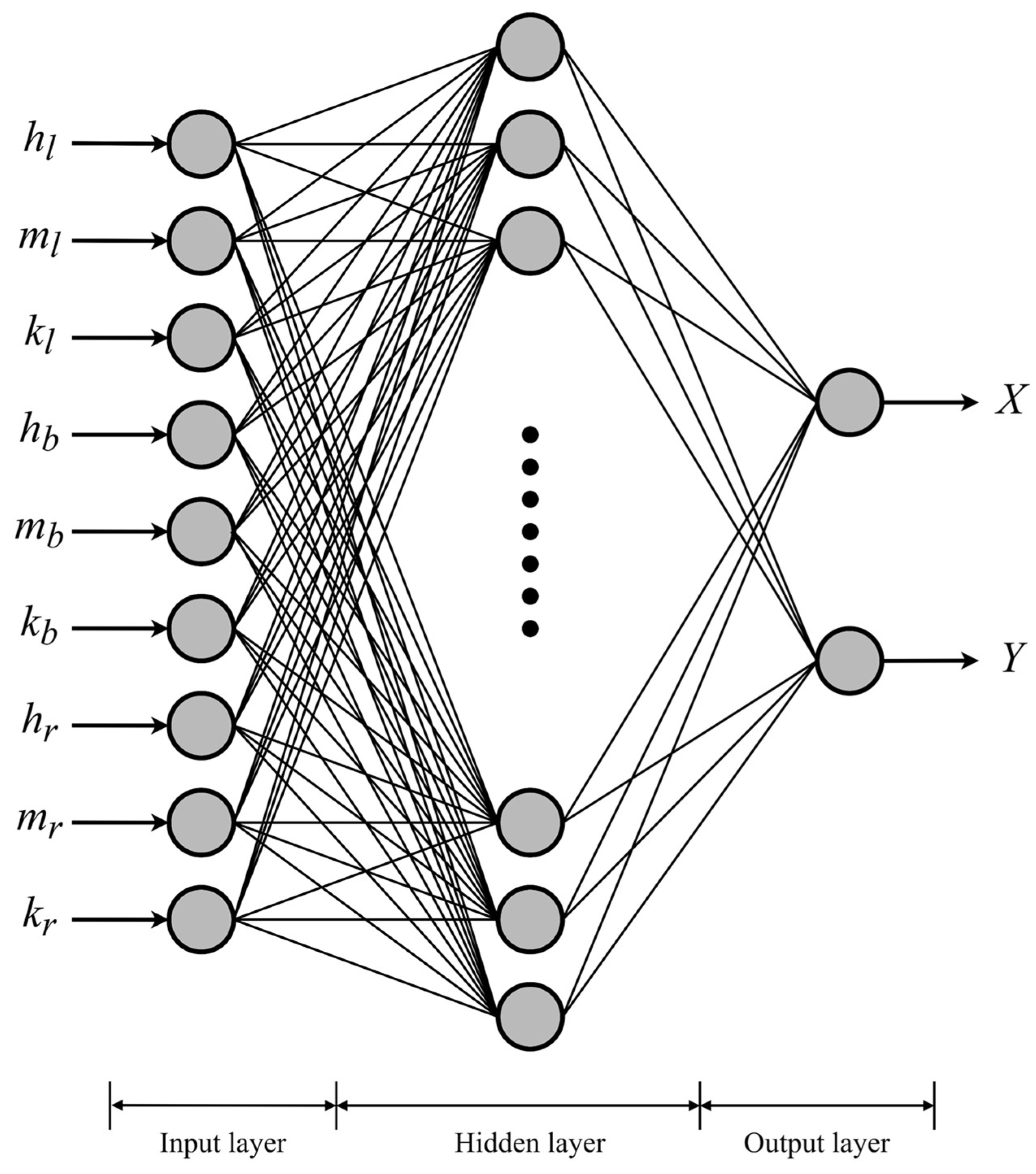
The multi-layered perceptron (MLP) [42] model is a traditional ANN model that was developed decades ago and has been widely adopted in different engineering disciplines due to its simple architecture and easy implementation. The architecture of the MLP used in this study is shown in Figure 3. The basic unit of an MLP model is an artificial neuron, which is a mathematical unit with multiple inputs and a single output. The first part of the neuron sums the input values, and the resulting sum passes to an activation function that produces the output. The neurons of the MLP model are arranged into three layers. The first layer is an input layer that receives input values from the user. Therefore, the number of neurons in this layer equals the number of input values plus one dummy input (not shown in Figure 3), where the input value equals one.
The second layer is called the hidden layer. The most common activation function of the neurons of this layer is the sigmoid function (i.e., y = 1 / ( 1 + e x ) ), which endows the model with nonlinearity. The number of hidden neurons in this layer determines the degree of nonlinearity. It was mathematically proven that an MLP with a single hidden layer and sufficient number of hidden neurons is a universal function approximator [43]. The number of hidden neurons can be estimated by different rules of thumb; the rule we adopted is given by the following equation, in which n h is the number of hidden neurons, N t r is the number of training samples, and N i n and N o u t are the numbers of inputs and outputs of the MLP model, respectively:
n h = N t r + N i n + N o u t 2
The neurons of the input layer and hidden layer are fully interlinked. A weighting factor is assigned to each of the links to scale the data fed from the input layer to the hidden layer. The last layer is the output layer, and its number of neurons equals the number of output values. The neurons of the hidden layers and output layers are also fully interlinked. Normally, the activation function of the neurons is linear; i.e., each output is a weighted sum of the outputs from neurons of the hidden layer.

2.3.2. Model Training

An MLP model can simulate the behaviours of nonlinear systems if the weights of the links between the layers are suitably selected. To this end, historical data are needed for training an MLP model; this training is typically performed via backpropagation, which is an error gradient-driven approach in which a weight is reduced if its increase causes an increase in the overall error. As backpropagation is an iterative process of adjusting the model parameters according to the output error of the last adjusted model, if all of the available samples are used to train a model, any error embedded in the samples will be fitted. This is denoted as overfitting and was prevented from occurring in this study by using the early-stop cross-validation training approach.
Three types of available samples are used for model training: training samples, validation samples and testing samples. Initially, the weights of all links of an MLP model (i.e., model parameters) are randomly assigned. Then, in each iteration of the backpropagation process (i.e., epoch), the intermediately trained model is applied to the training samples to evaluate the training error for adjusting the model parameters. Additionally, the intermediately trained model is applied to the validation samples to evaluate the validation error. If this error does not improve after a certain number of epochs (e.g., 200 epochs), the iteration of the backpropagation process is stopped, and the intermediate model with the minimum validation error is taken as the trained model. The performance of the model can be evaluated using the testing samples, which are unseen in the model-training phase.
If the number of available samples is limited, it is unreasonable to reserve a group of samples for evaluating system performance. Instead, we used leave-one-out validation, which is performed as follows. Initially, the first sample is selected as a testing sample, while the other samples are used to train the model. Upon the completion of model training, the trained model is applied to the first sample to evaluate the first prediction error. In the next step, the second sample is selected as the testing sample, while the other samples are used to train the model. Upon the completion of the model training, the trained model is applied to the second sample to evaluate the second prediction error. The procedure is repeated until the last prediction error is evaluated. If there are N samples, then N prediction errors are obtained via this leave-one-out approach.
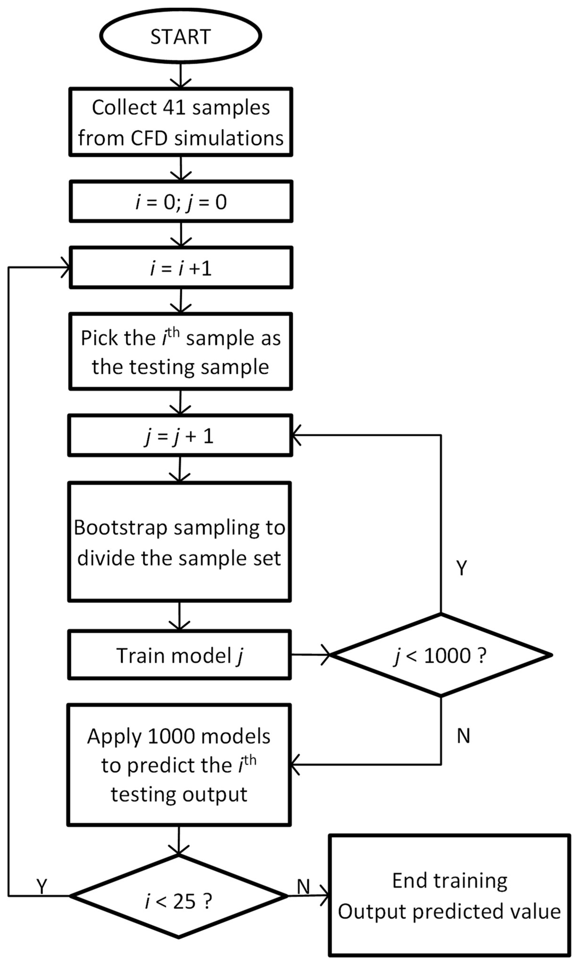
However, we note that there is randomisation in the above model training: i.e., the random sampling of the training and validation samples. Thus, it is possible that one may select “good” samples for model training, resulting in a good prediction. We prevented this from occurring by using a bagging approach [44], which increased the robustness of the model. Bagging was implemented in the leave-one-out validation process as follows. When one of the 41 samples was selected as the testing sample, the other samples were bootstrap-sampled (with replacement) to training samples (20 samples) and validation samples (20 samples) to train the MLP model. The same set of samples was bootstrap-sampled again to train another MLP model. This process was conducted 1000 times to create 1000 MLP models, which were fed with the input of the testing sample to produce 1000 prediction outputs. The final predicted output was the average of the 1000 prediction outputs. The overall model training is summarised in the flowchart in Figure 4.

3. Results and Discussion

3.1. Results of the MLP Prediction

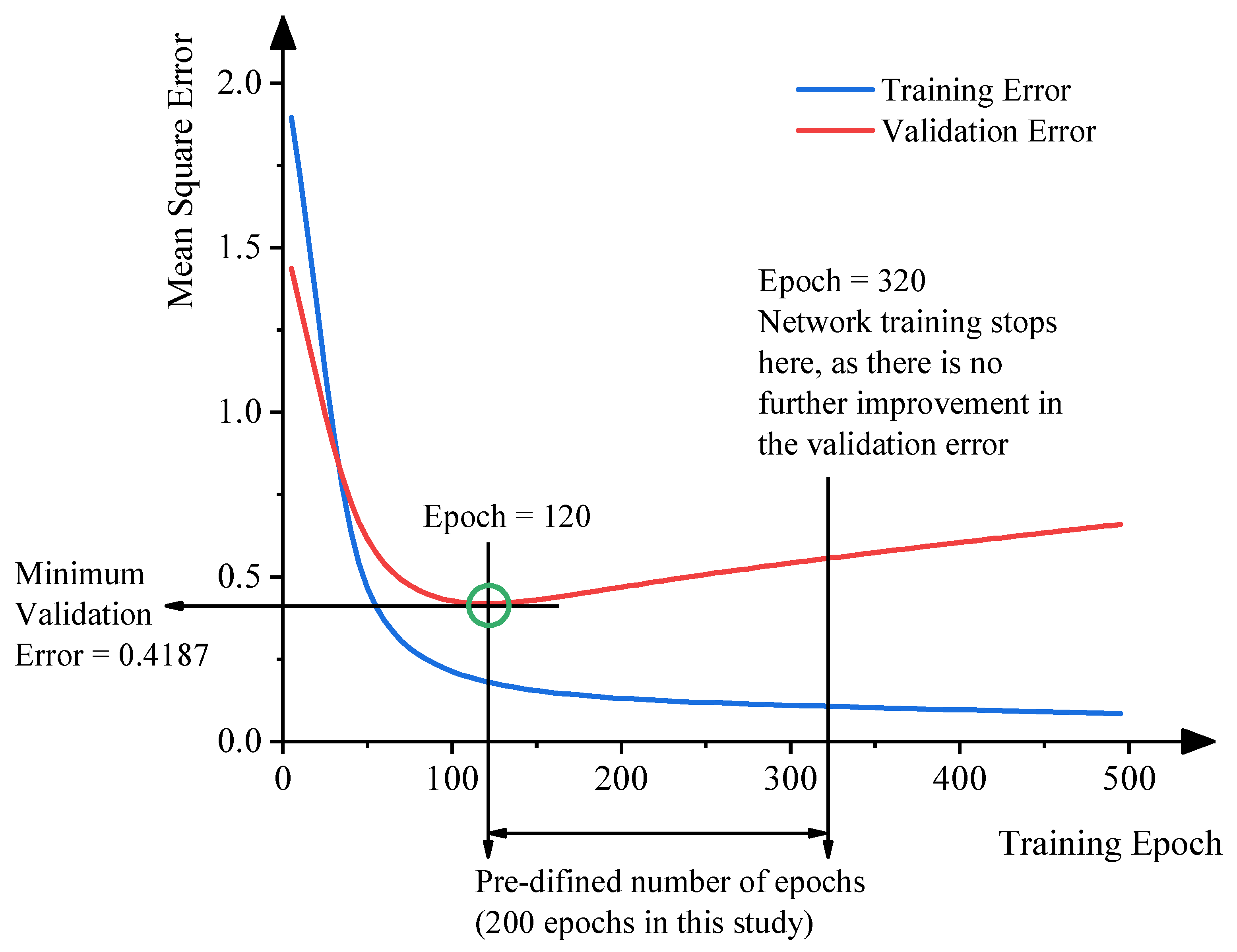
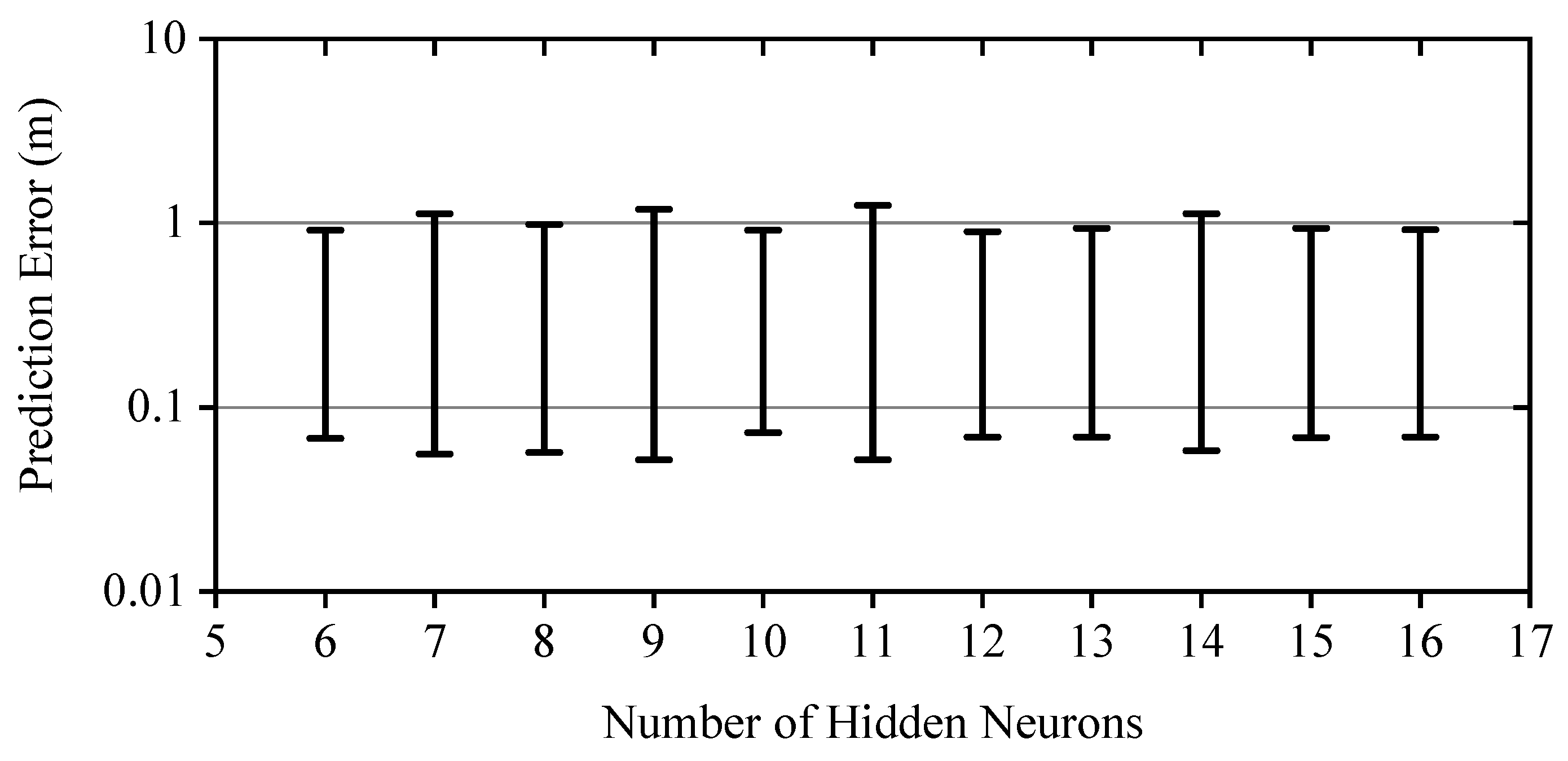
Figure 5 shows the changes in mean square error (MSE) versus the number of repetitions of the training loop. At the beginning of the training, since the network weights are randomly selected, the MSE is very high and then drops sharply by repeating the training loops. The network training stops at the green circle in Figure 5 since there is no further improvement in the validation error (after 200 epochs), and the network with the least error (i.e., epochs = 120) is chosen to approximate the output functions. The number of hidden neurons is another factor to influence the performance of an MLP model. The number of hidden neurons determines the performance of an MLP model. By use of Equation (4), the number of hidden neurons was estimated to be 11. The rule-of-thumb choice of the number of hidden neurons was justified in a sensitivity study, in which we carried out 11 trials to observe the performance of the MLP model with a fixed number of hidden neurons, ranging from 6 to 16 (i.e., 11 ± 5). In each trial, 25 prediction errors were obtained when adopting the leave-one-out approach. A log-normal distribution was assumed to fit these 25 prediction errors because each error (i.e., the distance between the predicted location and the actual location of the fire bed) was invariably positive and unbounded. The upper and lower limits of the 95% confidence interval of the distribution of each trial were obtained and are plotted in Figure 6. The fact that the confidence intervals overlapped each other demonstrates that no trial was superior; that is, the performance of the MLP model was not sensitive to the number of hidden neurons. Therefore, 11 hidden neurons were adopted in the MLP model.
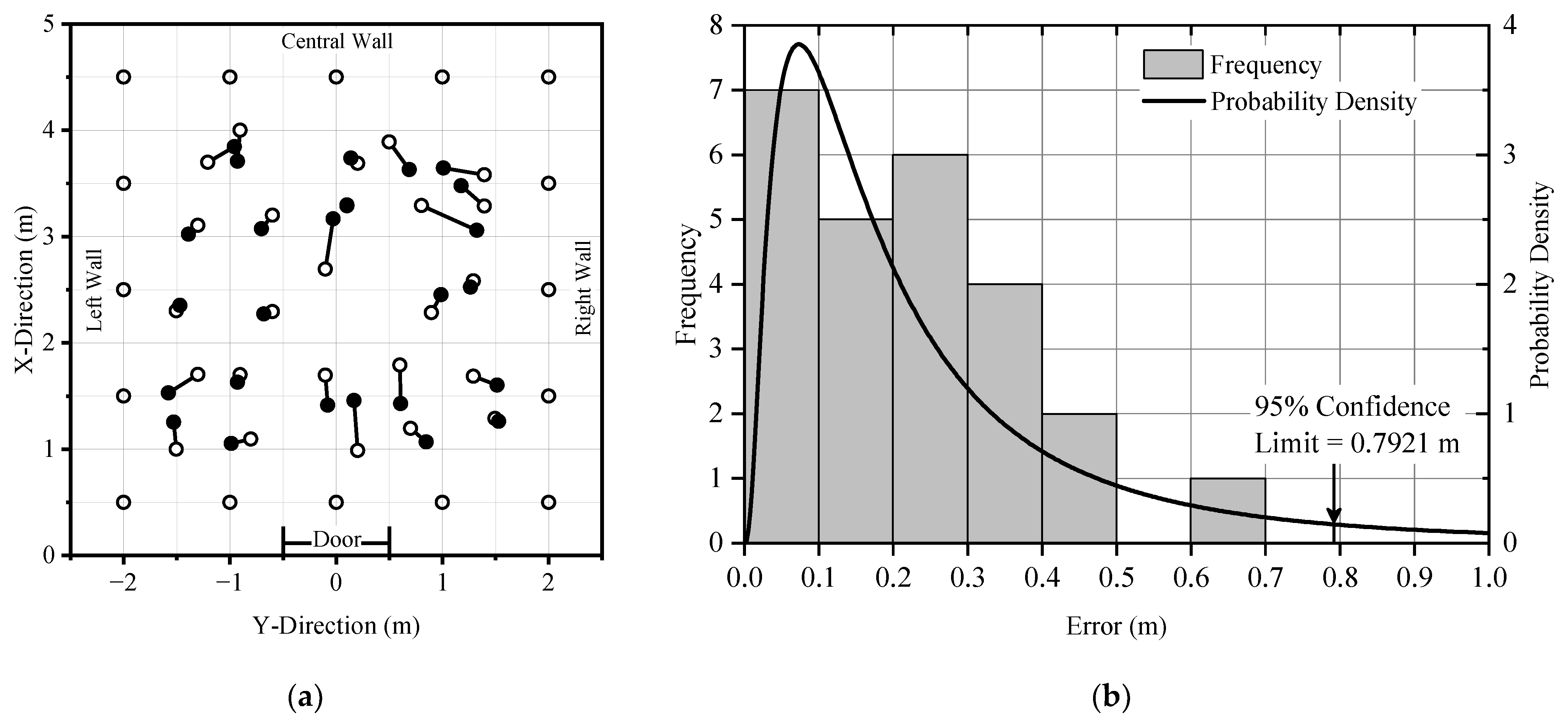
The model training approach shown in Figure 2b was adopted for the 41 samples extracted from the CFD simulations. The predictions are the locations of the fire beds reconstructed by the ANN model, and the actual and predicted locations of the fire beds are summarised in Figure 7a.
The histogram shown in Figure 7b summarises the 25 prediction errors and shows that all were less than 0.7 m. A log-normal distribution was applied to fit the error distribution, and the 95% left-tailed confidence limit was found to be 0.7921 m. Therefore, it was statistically justified that the prediction error of the bagging approach-supported MLP model was no more than 0.7921 m. In addition, the prediction by ANN could reduce the fire point to 1.97 m2 (area with 0.7921 m radius), which was only 7.8% of the room area (25 m2). A comparison of the error with the room size (i.e., 5 m × 5 m) with a single fire source, a fixed heat release rate (290 kW/m2) and a single opening indicated that the error is acceptable for engineering applications.

3.2. Effect of the Heat Release Rate on the Prediction Results

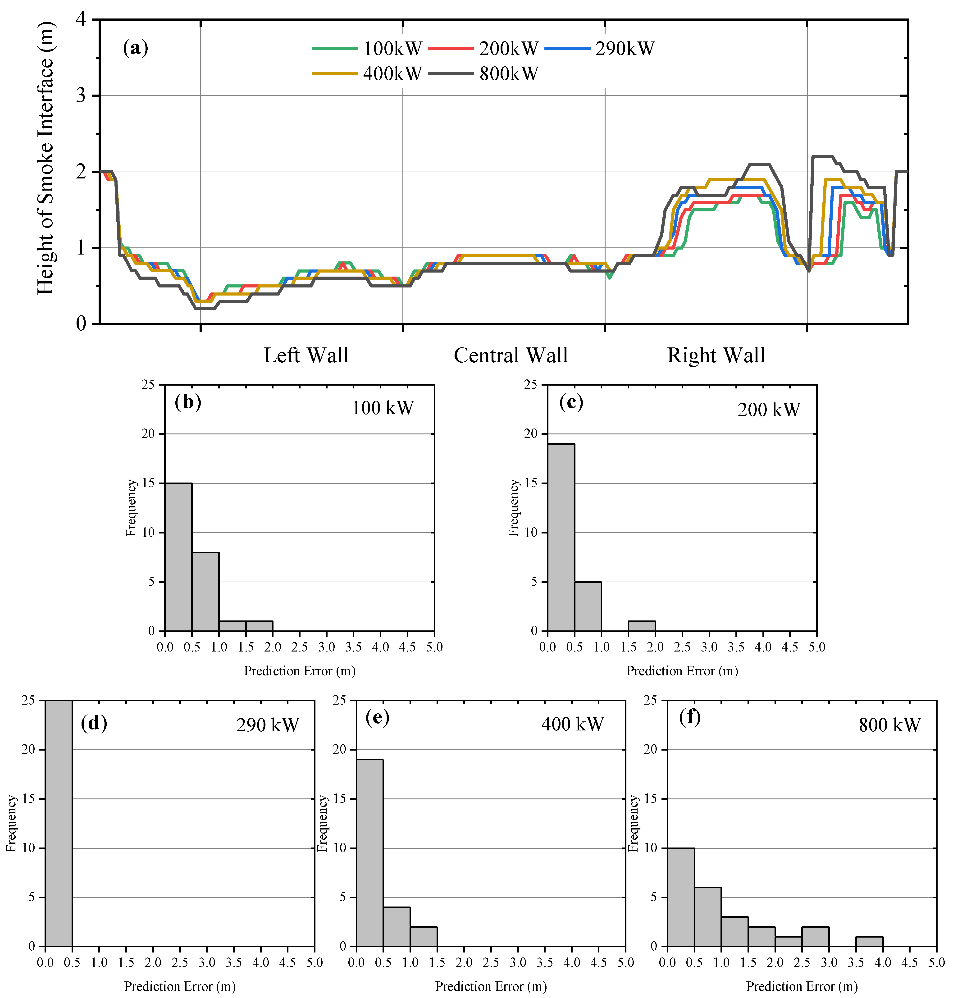
We also investigated the effect of the heat release rate of a fire on the soot patterns on the walls. Thus, we carried out CFD simulations using heat release rates of 100, 200, 400 and 800 kW/m2, in addition to a heat release rate of 290 kW/m2, with the same room geometry and same fire location (X = 3.5 m; Y = 1.0 m). The results are presented in Figure 8, which shows the height of the smoke interface on the four compartment walls. The fire was located closer to the left wall, and we thus observed that the smoke interface on the left wall was lower than that on the right wall. An increase in the heat release rate magnified the deviation in the smoke interface profile between walls, but the overall profiles were similar for the different heat release rates. We thus believe that the ANN model trained using the data for the 290 kW/m2 fire is also applicable to reconstructing fire source locations in fire scenarios having the same room geometry but different heat release rates.
We used the 41 samples shown in Figure 2b with a heat release rate of 290 kW/m2 to train 1000 MLP models through the random extraction of training and validation samples. The 1000 MLP models were combined by adopting the bagging ensemble approach. The trained ensemble MLP model was then applied to predict the fire source locations from the patterns of soot deposited on the walls for different heat release rates (i.e., 100, 200, 400 and 800 kW) in the fast-growth t-squared fire model and different fire source locations. The prediction errors are summarised in Figure 8, which shows that the prediction error was the lowest (less than 0.5 m) for a heat release rate of 290 kW/m2. This result was expected because the same set of data was used to train the ensemble MLP model. The model performances were similar for heat release rates of 100, 200 and 400 kW/m2, with all prediction errors being less than 2 m. From an engineering point of view, this prediction error is acceptable for practical application. In contrast, the prediction error was large for a heat release rate of 800 kW, reaching a maximum value of 3.7 m; this might have been due to the large difference between the heat release rates of the training samples (i.e., 290 kW/m2) and testing samples (i.e., 800 kW/m2).

3.3. Experiments in a Scaled Space

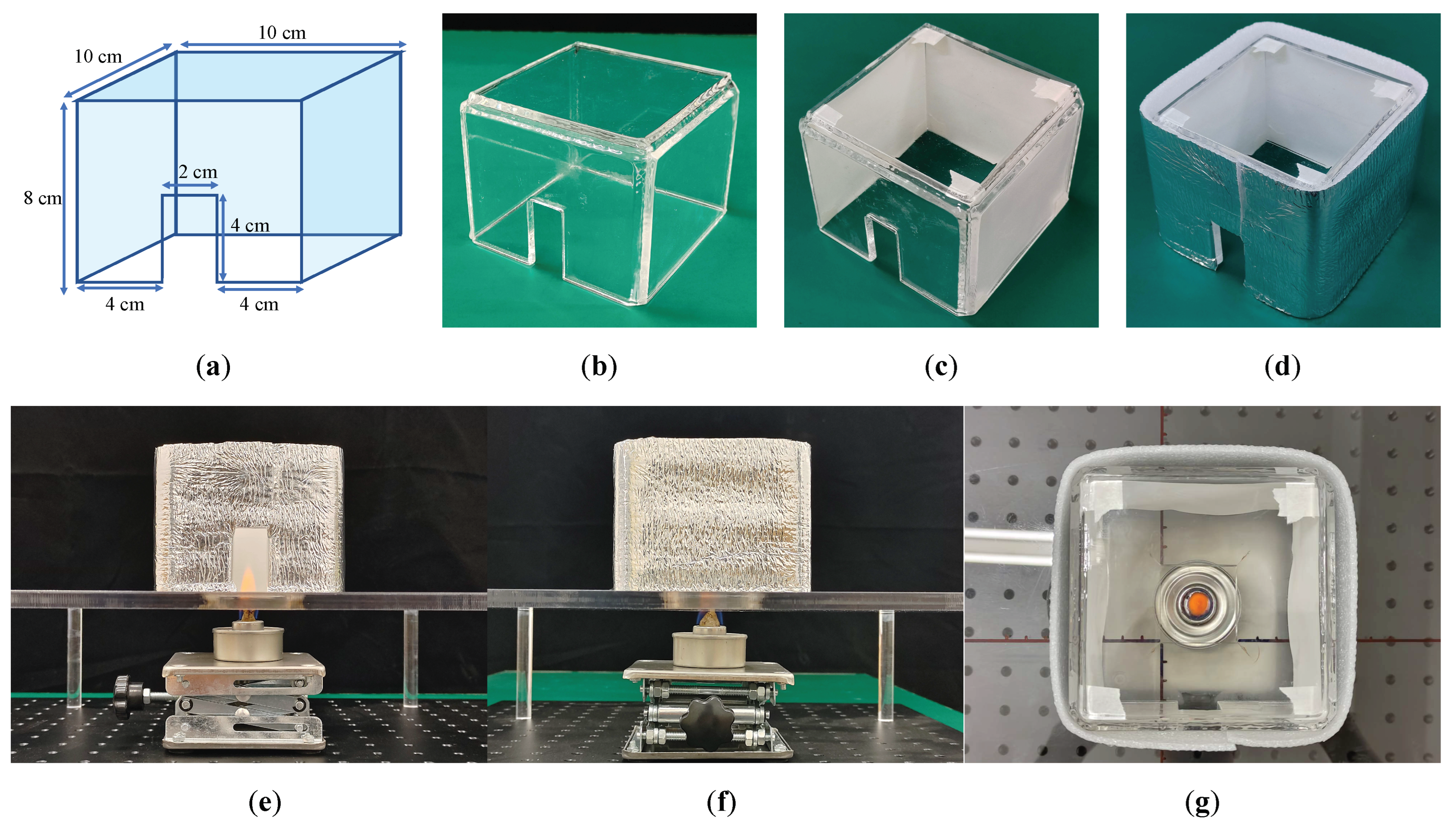
We performed comprehensive combustion experiments to verify the performance of our ANN model. As a 1:1 experiment would incur a high cost and require much time and space, we scaled down the fire compartment presented in FDS by a ratio of 1:50. Thus, in contrast to the simulations, which we conducted in a fire room with dimensions of 5 m × 5 m × 4 m, we conducted these experiments in a scaled fire compartment with dimensions of 0.1 m × 0.1 m × 0.08 m. The structure and a photograph of the scaled fire compartment are shown in Figure 9a,b, respectively. The compartment was made from tempered glass with high-temperature assistance. Thermal paper that changed colour once heated was attached to the inner wall of the fire compartment, as shown in Figure 9c, and insulation material was wrapped around the exterior of the fire compartment to reduce heat loss, as shown in Figure 9d. Ethylene glycol was used as fuel because it has high calorific value (i.e., 1180.26 kJ/mol), is inexpensive and is easy to obtain. Photographs of the combustion experiment taken from different views are shown in Figure 9e–g. The fuel was placed on an optical plate that had a hole with a diameter of 2.5 cm, a scale (Figure 9g) was drawn for precise positioning, and the flame height was controlled by a lifting platform (Figure 9e,f). An experiment was stopped when the pattern of soot deposited on the thermal paper no longer changed.
A new software program, FSRSP (refer to Fire source reconstructed by soot pattern), was developed to accurately recognise the smoke interface of the soot pattern on thermal paper and then predict the fire location by using the proposed ANN model. As shown in Figure 10, once the thermal papers on the left, central and right walls were uploaded into the software FSRSP, the embedded OpenCV module was used to extract the smoke interface of the soot pattern (blue lines), and the experimental data were scaled (i.e., enlarged) by a factor of 50:1 to observe the scale rule and to maintain consistency with FDS. Then the quadratic fitting results (red lines) were calculated and used to predict and draw the fire location by using the aforementioned ANN model shown on the lower right corner of Figure 10. More details on the usage of the new software FSRSP are presented in Supplementary Materials.
We conducted an experiment five times for each fire location. Figure 11 compares the profiles of the smoke interface of the experimental and FDS soot patterns. The five results of the experiment conducted with the fire source at the centre of the fire compartment showed stability, i.e., there was a similar trend in the variation of the soot pattern on the left, central and right walls, and this was the same trend obtained by FDS.
We next took the average of the five results of the smoke interface of the soot pattern for the different six-source locations (presented in Table 2). The average height of the smoke interface, average gradient of the smoke interface and average curvature of the smoke interface were then calculated as the input of the ANN model introduced in Section 3.3. The predictions obtained were the locations of the fire source reconstructed by the ANN model, and the differences between the scaled actual source locations and the predicted source locations are presented in Table 2. The results show that the differences between the scaled actual values and predicted values were less than 1 m for all of the source positions. In particular, when the fire was located at the centre of the fire compartment, the difference between the actual and predicted locations was only 0.17 m. This demonstrates the feasibility of using the ANN model to reconstruct the location of a fire source in engineering applications.

4. Conclusions

A fire source location is usually estimated by fire investigators at a fire scene according to their experience. In this study, we developed an objective approach for fire source location by developing an ANN model for reconstructing the location of a fire source from the patterns of soot deposited on walls. Samples for the ANN model were collected using FDS, which is a useful tool with which to simulate fire development and patterns of soot deposition on walls. A data preprocessor was used to transform the numerical simulation results to a usable format, and bootstrap aggregation was adopted to improve the model prediction performance, which was evaluated by the leave-one-out approach. The 95% left-tailed confidence limit was 0.7921 m; i.e., the prediction error of the ANN model was no more than 0.7921 m. Additionally, an increase in the heat release rate magnified the difference between the smoke interface profiles of walls, but the profiles for different heat release rates were similar to each other.
To verify the ANN model, we conducted a series of combustion experiments in a fire compartment that was geometrically similar for a range of fire source locations. A new software program, FSRSP, was developed to accurately recognise the smoke interface of the soot pattern on thermal paper and then predict the fire location. The results showed that the difference between the scaled actual location and the predicted location was less than 1 m at all positions and was a minimum (i.e., 0.17 m) when the fire source was at the centre of the fire compartment. Thus, the ANN model is acceptable for reconstructing the location of a fire source in engineering applications. The newly developed software, FSRSP, can assist fire investigators in performing forensic work in an objective way.
In conclusion, the utilization of an ANN in fire investigation efforts revolutionizes the traditional approach to fire investigation. With its data-driven insights and objective analyses, the ANN serves as a valuable asset in modern firefighting. By quickly and accurately narrowing down potential fire locations, the ANN approach empowers firefighters to respond swiftly and decisively, thereby enhancing the overall efficiency and effectiveness of fire investigations.
Our study still has some limitations. First, the training samples were relatively homogeneous: we only set up samples with different fire locations in a single room, which limited the generalisation ability of the ANN model. Therefore, further design in terms of fire power, fuel type and room type can be performed to increase the diversity of the samples and yield better generalisation ability of the ANN model. Room types can be designed in terms of room aspect ratio, exit locations, and ventilation. Second, the proposed ANN model and developed software, FSRSP, need to be examined in a real building fire. Finally, except for the ANN model, deep learning methods such as convolution neural network (CNN) and long short-term memory network (LSTM) models can also be used to predict fire location or fire power.

Supplementary Materials

Code and documentation related to the FSRSP software (version 1.0) can be found at: https://github.com/HTBCF/FSRSP (accessed on 2 August 2023).

Author Contributions

Conceptualization, M.S. and E.W.M.L.; methodology, M.S.; software, H.L.; validation, M.S., H.L. and Z.Z.; formal analysis, M.S.; investigation, H.L.; resources, M.S.; data curation, H.L.; writing—original draft preparation, M.S.; writing—review and editing, H.L.; visualization, H.L.; supervision, E.W.M.L.; project administration, M.S.; funding acquisition, M.S. All authors have read and agreed to the published version of the manuscript.

Funding

This work was supported by the National Natural Science Foundation of China (No. 72104254), Hubei Provincial Natural Science Foundation of China (No. 2022CFB469), and the Research Start-up Foundation of South-Central Minzu University (YZZ21002).

Institutional Review Board Statement

Not applicable.

Informed Consent Statement

Not applicable.

Data Availability Statement

Data will be made available on request.

Acknowledgments

We are grateful to Key Laboratory of Cyber-Physical Fusion Intelligent Computing (South-Central Minzu University) and Hubei Provincial Engineering Research Center for Intelligent Management of Manufacturing Enterprises for the laboratory aspects of this study.

Conflicts of Interest

The authors declare no conflict of interest.

References

  1. Fire Services Department—Hong Kong Fire Services Review 2011. Available online: https://www.hkfsd.gov.hk/eng/publications/review/review_11.html (accessed on 20 October 2022).
  2. Milke, J.A.; McAvoy, T.J. Analysis of Signature Patterns for Discriminating Fire Detection with Multiple Sensors. Fire Technol. 1995, 31, 120–136. [Google Scholar] [CrossRef]
  3. Lee, W.M.; Yuen, K.K.; Lo, S.M.; Lam, K.C. Prediction of Sprinkler Actuation Time Using the Artificial Neural Networks. J. Build. Surv. 2000, 2, 10–13. [Google Scholar]
  4. Lee, E.; Yuen, R.; Lo, S.M.; Lam, K.C. Probabilistic Inference with Maximum Entropy for Prediction of Flashover in Single Compartment Fire. Adv. Eng. Inform. 2002, 16, 179–191. [Google Scholar] [CrossRef]
  5. Lee, E.W.M.; Lim, C.P.; Yuen, R.K.K.; Lo, S.M. A Hybrid Neural Network Model for Noisy Data Regression. IEEE Trans. Syst. Man Cybern. Part B 2004, 34, 951–960. [Google Scholar] [CrossRef]
  6. Lee, E.W.M.; Yuen, R.K.K.; Lo, S.M.; Lam, K.C.; Yeoh, G.H. A Novel Artificial Neural Network Fire Model for Prediction of Thermal Interface Location in Single Compartment Fire. Fire Saf. J. 2004, 39, 67–87. [Google Scholar] [CrossRef]
  7. Lee, E.W.M.; Lee, Y.Y.; Lim, C.P.; Tang, C.Y. Application of a Noisy Data Classification Technique to Determine the Occurrence of Flashover in Compartment Fires. Adv. Eng. Inform. 2006, 20, 213–222. [Google Scholar] [CrossRef]
  8. Yuen, R.K.; Lee, E.W.; Lo, S.; Yeoh, G. Prediction of Temperature and Velocity Profiles in a Single Compartment Fire by an Improved Neural Network Analysis. Fire Saf. J. 2006, 41, 478–485. [Google Scholar] [CrossRef]
  9. Asgary, A.; Sadeghi Naini, A.; Levy, J. Modeling the Risk of Structural Fire Incidents Using a Self-Organizing Map. Fire Saf. J. 2012, 49, 1–9. [Google Scholar] [CrossRef]
  10. Xu, J.; Zhao, J.; Wang, W.; Liu, M. Prediction of Temperature of Tubular Truss under Fire Using Artificial Neural Networks. Fire Saf. J. 2013, 56, 74–80. [Google Scholar] [CrossRef]
  11. Barros-Daza, M.J.; Luxbacher, K.D.; Lattimer, B.Y.; Hodges, J.L. Real Time Mine Fire Classification to Support Firefighter Decision Making. Fire Technol. 2022, 58, 1545–1578. [Google Scholar] [CrossRef]
  12. Buffington, T.; Cabrera, J.-M.; Kurzawski, A.; Ezekoye, O.A. Deep-Learning Emulators of Transient Compartment Fire Simulations for Inverse Problems and Room-Scale Calorimetry. Fire Technol. 2021, 57, 2859–2885. [Google Scholar] [CrossRef]
  13. Lattimer, B.Y.; Hodges, J.L.; Lattimer, A.M. Using Machine Learning in Physics-Based Simulation of Fire. Fire Saf. J. 2020, 114, 102991. [Google Scholar] [CrossRef]
  14. Gu, W.; Bai, S.; Kong, L. A Review on 2D Instance Segmentation Based on Deep Neural Networks. Image Vis. Comput. 2022, 120, 104401. [Google Scholar] [CrossRef]
  15. Otter, D.W.; Medina, J.R.; Kalita, J.K. A Survey of the Usages of Deep Learning for Natural Language Processing. IEEE Trans. Neural Netw. Learn. Syst. 2021, 32, 604–624. [Google Scholar] [CrossRef] [Green Version]
  16. Zhang, F.; Shi, L.; Liu, S.; Zhang, C.; Liu, Z. CFD-Based Validation Study on the Fire Prevention Wisdom of Ancient Village Houses in Western Hunan. Fire 2023, 6, 144. [Google Scholar] [CrossRef]
  17. Delémont, O.; Martin, J.-C. Application of Computational Fluid Dynamics Modelling in the Process of Forensic Fire Investigation: Problems and Solutions. Forensic Sci. Int. 2007, 167, 127–135. [Google Scholar] [CrossRef]
  18. Hofmann, A.; Muehlnikel, R. Experimental and Numerical Investigation of Fire Development in a Real Fire in a Five-Storey Apartment Building. Fire Mater. 2011, 35, 453–462. [Google Scholar] [CrossRef]
  19. Manea, F.; Ghicioi, E.; Suvar, M.C.; Prodan, M.; Vlasin, N.I.; Suvar, N.S.; Vlase, T. FDS Results for Selecting the Right Scenario in the Case of a Building Fire: A Case Study. Fire 2022, 5, 198. [Google Scholar] [CrossRef]
  20. Yan, X.; Yang, H.; Mo, H.; Xie, Y.; Jin, Z.; Zhou, Y. Numerical Simulation on the Smoke Prevention Performance of Air Curtains in an Island-Type Subway Station. Fire 2023, 6, 177. [Google Scholar] [CrossRef]
  21. Li, Y.; Huang, F.; Ma, C.; Tang, K. A Simulation Study on the Smoke Control Effect with Different Smoke Exhaust Patterns and Longitudinal Air Supply for Ultra-Wide Tunnels. Fire 2022, 5, 72. [Google Scholar] [CrossRef]
  22. Chi, J.-H. Metallographic Analysis and Fire Dynamics Simulation for Electrical Fire Scene Reconstruction. J. Forensic Sci. 2012, 57, 246–249. [Google Scholar] [CrossRef]
  23. Barshick, S.-A. Analysis of Accelerants and Fire Debris Using Aroma Detection Technology. J. Forensic Sci. 1998, 43, 284–293. [Google Scholar] [CrossRef] [Green Version]
  24. Biedermann, A.; Taroni, F.; Delemont, O.; Semadeni, C.; Davison, A.C. The Evaluation of Evidence in the Forensic Investigation of Fire Incidents (Part I): An Approach Using Bayesian Networks. Forensic Sci. Int. 2005, 147, 49–57. [Google Scholar] [CrossRef]
  25. Lu, W.; Rankin, J.G.; Bondra, A.; Trader, C.; Heeren, A.; Harrington, P.d.B. Ignitable Liquid Identification Using Gas Chromatography/Mass Spectrometry Data by Projected Difference Resolution Mapping and Fuzzy Rule-Building Expert System Classification. Forensic Sci. Int. 2012, 220, 210–218. [Google Scholar] [CrossRef] [PubMed]
  26. Zhang, G.; Zhou, X.; Zhu, G.; Yan, S. A New Accident Analysis and Investigation Model for the Complex Building Fire Using Numerical Reconstruction. Case Stud. Therm. Eng. 2019, 14, 100426. [Google Scholar] [CrossRef]
  27. Overholt, K.J.; Ezekoye, O.A. Quantitative Testing of Fire Scenario Hypotheses: A Bayesian Inference Approach. Fire Technol. 2015, 51, 335–367. [Google Scholar] [CrossRef]
  28. Freitas, R.A.; Rodrigues, J.P.C. A Fire Investigation Methodology for Buildings. Archit. Struct. Constr. 2022, 2, 269–290. [Google Scholar] [CrossRef]
  29. Hartman, J.R.; Beyler, A.P.; Riahi, S.; Beyler, C.L. Smoke Oxidation Kinetics for Application to Prediction of Clean Burn Patterns. Fire Mater. 2012, 36, 177–184. [Google Scholar] [CrossRef]
  30. Ciro, W.D.; Eddings, E.G.; Sarofim, A.F. Experimental and Numerical Investigation of Transient Soot Buildup on a Cylindrical Container Immersed in a Jet Fuel Pool Fire. Combust. Sci. Technol. 2006, 178, 2199–2218. [Google Scholar] [CrossRef]
  31. Cohan, B.D. Verification and Validation of a Candidate Soot Deposition Model in Fire Dynamics Simulator Version 5.5.1. Master’s Thesis, University of Maryland, College Park, MD, USA, 2010. [Google Scholar]
  32. Riahi, S.; Beyler, C.L.; Hartman, J. Wall Smoke Deposition from a Hot Smoke Layer. Fire Technol. 2013, 49, 395–409. [Google Scholar] [CrossRef]
  33. Talbot, L.; Cheng, R.K.; Schefer, R.W.; Willis, D.R. Thermophoresis of Particles in a Heated Boundary Layer. J. Fluid Mech. 1980, 101, 737–758. [Google Scholar] [CrossRef] [Green Version]
  34. Papavergos, P.G.; Hedley, A.B. Particle Deposition Behavior from Turbulent Flows. Chem. Eng. Res. Des. 1984, 62, 275–295. [Google Scholar]
  35. McGrattan, K.; Hostikka, S.; McDermott, R.; Floyd, J.; Weinschenk, C.; Overholt, K. Fire Dynamics Simulator Technical Reference Guide Volume 1: Mathematical Model; NIST Special Publication: Baltimore, MD, USA, 2013. [CrossRef]
  36. Brock, J.R. On the Theory of Thermal Forces Acting on Aerosol Particles. J. Colloid Sci. 1962, 17, 768–780. [Google Scholar] [CrossRef]
  37. Floyd, J.; Overholt, K.; Ezekoye, O. Soot Deposition and Gravitational Settling Modeling and the Impact of Particle Size and Agglomeration. Fire Saf. Sci. 2014, 11, 174. [Google Scholar] [CrossRef]
  38. He, Y.; Fernando, A.; Luo, M. Determination of Interface Height from Measured Parameter Profile in Enclosure Fire Experiment. Fire Saf. J. 1998, 31, 19–38. [Google Scholar] [CrossRef]
  39. Wright, E.M. Adaptive Control Processes: A Guided Tour. Math. Gaz. 1962, 46, 160–161. [Google Scholar] [CrossRef]
  40. Brinson, A.; Johnson, P.; Kip, S.; Torero, J.; Lange, D.; Salomonsson, T. Fire Safety Engineering: Comparison of FSE Guidance Documents and Assessment Criteria Special Report; The Warren Centre for Advanced Engineering: Sydney, Australia, 2019; ISBN 978-0-648-50292-0. [Google Scholar]
  41. McGrattan, K. Verification and Validation of Selected Fire Models for Nuclear Power Plant Applications: Fire Dynamics Simulator (FDS). Available online: https://www.nrc.gov/reading-rm/doc-collections/nuregs/staff/sr1824/v7/index.html (accessed on 30 July 2023).
  42. Rosenblatt, F. Principles of Neurodynamics: Perceptrons and the Theory of Brain Mechanisms; Spartan Books: Washington, DC, USA, 1962. [Google Scholar]
  43. Hornik, K.; Stinchcombe, M.; White, H. Multilayer Feedforward Networks Are Universal Approximators. Neural Netw. 1989, 2, 359–366. [Google Scholar] [CrossRef]
  44. Breiman, L. Bagging Predictors. Mach. Learn. 1996, 24, 123–140. [Google Scholar] [CrossRef] [Green Version]
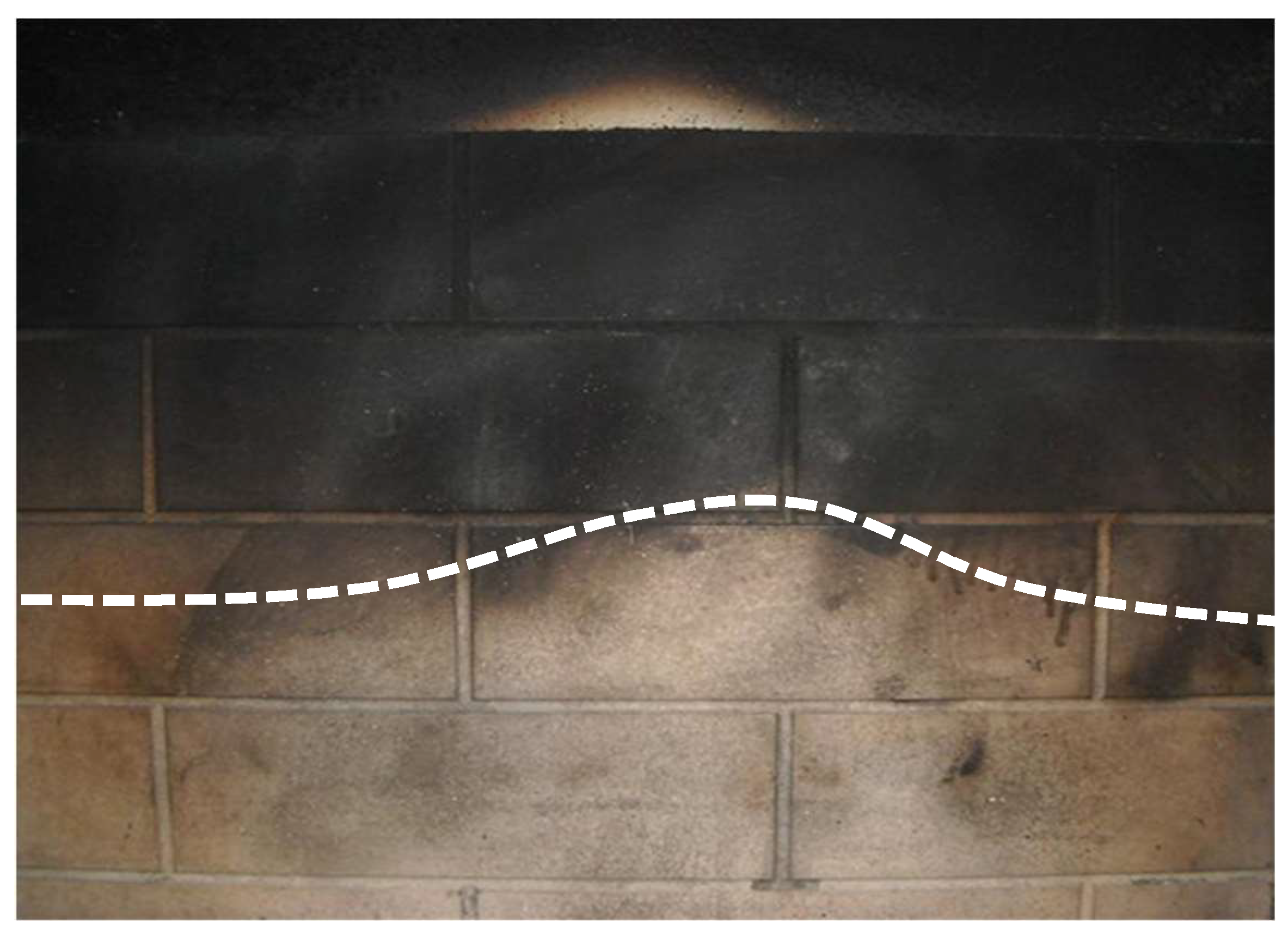
Figure 1. Example showing that the pattern of soot deposition on a wall does not clearly demarcate an upper smoke zone and lower cold-air zone. The white broken line demarcates the upper smoke layer and lower clear layer.
Fire 06 00303 g001
Figure 2. Geometry of the fire compartment and floor plan of fire source: (a) Geometry configurations and (b) floor plan of fire source locations in 41 cases. The locations marked with circles are boundary locations, whereas those marked with crosses are randomly placed inside of the boundary locations.
Fire 06 00303 g002
Figure 3. Architecture of the MLP used in this study.
Fire 06 00303 g003
Figure 4. Flowchart showing the training algorithm incorporating leave-one-out validation and bagging, where i represents the ith sample of the 25 random source locations shown in Figure 2b and j is the index of the model trained by the samples obtained through bootstrap resampling.
Fire 06 00303 g004
Figure 5. The changes in prediction error versus the number of repetitions of the training loop (epoch).
Fire 06 00303 g005
Figure 6. Prediction errors of the MLP model with various numbers of hidden neurons.
Fire 06 00303 g006
Figure 7. Results of the MLP prediction. (a) The difference between actual locations and predicted locations: The open and solid circles are the actual locations and predicted locations of the fire beds, respectively. (b) Statistical analysis of the MLP prediction error showing that the prediction error was no more than 0.7921 m at a 95% confidence level.
Fire 06 00303 g007
Figure 8. Prediction results under different heat release rates. (a) Profiles of the smoke interface of the pattern of soot deposition on the compartment walls at different heat release rates with the fire source located at (X = 3.5 m, Y = 1.0 m) and summary of prediction errors at different heat release rates: (b) 100 kw, (c) 200 kw, (d) 290 kw, (e) 400 kw and (f) 800 kw.
Fire 06 00303 g008
Figure 9. Geometry and photographs taken during the combustion experiment. Scaled fire compartment: (a) geometry, (b) photograph of the fire compartment, (c) photograph showing thermal paper attached to the inner wall, (d) photograph showing insulation wrapped around the exterior wall and photographs taken from different views: (e) front view, (f) left view and (g) top view.
Fire 06 00303 g009
Figure 10. Screen shot of the software program FSRSP: blue lines represent the smoke interface of the soot pattern extracted by the OpenCV module, red lines represent quadratic fitting results and cross mark represents fire location predicted by the ANN model.
Fire 06 00303 g010
Figure 11. The profiles of the smoke interface of the experimental and FDS soot patterns: (a) left wall, (b) central wall and (c) right wall.
Fire 06 00303 g011
Table 1. Summary of the input and output parameters of the ANN model.
TypeNo.Description
Inputs1Average height of the smoke interface on the left wall ( h l )
2Average slope of the smoke interface on the left wall ( m l )
3Average curvature of the smoke interface on the left wall ( κ l )
4Average height of the smoke interface on the central wall ( h b )
5Average slope of the smoke interface on the central wall ( m b )
6Average curvature of the smoke interface on the central wall ( κ b )
7Average height of smoke interface on the right wall ( h r )
8Average slope of the smoke interface on the right wall ( m r )
9Average curvature of the smoke interface on the right wall ( κ r )
Outputs1X-coordinate of the fire bed centre ( X )
2Y-coordinate of the fire bed centre ( Y )
Table 2. Scaled real location, scaled predicted location and the difference between them for different fire source locations.
Experiment No.Fire Source Location in Experiment
(cm, cm)
Scaling of Fire Source Location
(m, m)
Predictions Generated by the ANN Model
(m, m)
Difference between the Actual and Average Predicted Locations
(m)
1(5.00, 0.00)(2.50, 0.00)(2.36, −0.09)0.17
2(7.00, 2.00)(3.50, 1.00)(3.22, 0.37)0.68
3(7.00, 0.00)(3.50, 0.00)(2.87, −0.18)0.66
4(3.00, 0.00)(1.50, 0.00)(1.73, 0.12)0.26
5(5.00, 2.00)(2.50, 1.00)(2.40, −0.01)0.99
6(3.00, 2.00)(1.50, 1.00)(1.74, 0.18)0.85
Disclaimer/Publisher’s Note: The statements, opinions and data contained in all publications are solely those of the individual author(s) and contributor(s) and not of MDPI and/or the editor(s). MDPI and/or the editor(s) disclaim responsibility for any injury to people or property resulting from any ideas, methods, instructions or products referred to in the content.