Multi-Indices Diagnosis of the Conditions That Led to the Two 2017 Major Wildfires in Portugal

Abstract

Forest fires, though part of a natural forest renewal process, when frequent and on a large -scale, have detrimental impacts on biodiversity, agroforestry systems, soil erosion, air, and water quality, infrastructures, and the economy. Portugal endures extreme forest fires, with a record extent of burned areas in 2017. These complexes of extreme wildfire events (CEWEs) concentrated in a few days but with highly burned areas are, among other factors, linked to severe fire weather conditions. In this study, a comparison between several fire danger indices (named ‘multi-indices diagnosis’) is performed for the control period 2001–2021, 2007 and 2017 (May–October) for the Fire Weather Index (FWI), Burning Index (BI), Forest Fire Danger Index (FFDI), Continuous Haines Index (CHI), and the Keetch–Byram Drought Index (KBDI). Daily analysis for the so-called Pedrógão Grande wildfire (17 June) and the October major fires (15 October) included the Spread Component (SC), Ignition Component (IC), Initial Spread Index (ISI), Buildup Index (BUI), and the Energy Release Component (ERC). Results revealed statistically significant high above-average values for most of the indices for 2017 in comparison with 2001–2021, particularly for October. The spatial distribution of BI, IC, ERC, and SC had the best performance in capturing the locations of the two CEWEs that were driven by atmospheric instability along with a dry environment aloft. These results were confirmed by the hotspot analysis that showed statistically significant intense spatial clustering between these indices and the burned areas. The spatial patterns for SC and ISI showed high values associated with high velocities in the spread of these fires. The outcomes allowed us to conclude that since fire danger depends on several factors, a multi-indices diagnosis can be highly relevant. The implementation of a Multi-index Prediction Methodology should be able to further enhance the ability to track and forecast unique CEWEs since the shortcomings of some indices are compensated by the information retrieved by others, as shown in this study. Overall, a new forecast method can help ensure the development of appropriate spatial preparedness plans, proactive responses by civil protection regarding firefighter management, and suppression efforts to minimize the detrimental impacts of wildfires in Portugal.

1. Introduction

Forest fires are one of the most severe natural disasters that periodically affect Mediterranean countries [1,2,3,4,5,6], as well as countries and regions with Mediterranean-like climates, such as California in the south-eastern United States of America (USA) [7,8,9], or in more dry climates like Australia [10]. In the Mediterranean region, the climate is characterized by Mediterranean hot–(CSa) or warm-summers (CSb) [11], as well as dry summers (B type, following the Köppen–Geiger Climatic Classification [12]), and this is a key factor—influenced by the nature and magnitude of climate change (exposure) and forestry policies—that partially explains the susceptibility of this region to wildfires. Within the Mediterranean area, Portugal is one of the most affected [13,14,15] with major losses in its ecosystems and agroforestry systems [16,17] but also in infrastructures [18] and, unfortunately, human lives. Therefore, a better understanding of the underlying danger factors and danger indices is of utmost relevance.

The significance of meteorological conditions for the incidence of conditions prone to the occurrence of forest fires is well known [19,20,21,22,23]. Therefore, the ability to anticipate their impact on daily fire occurrence and related behavior is one of the major goals of researchers in this field [24,25]. As a result, several fire danger evaluation indices or methods have been developed and adapted in different regions of the world [26,27,28,29,30]. In Portugal, the Canadian Forest Service Fire Weather Index (FWI) System is the only fire danger index used and is calculated with surface meteorological parameters [31,32,33,34,35]. Its forecast is given by the Instituto Português do Mar e da Atmosfera (IPMA) [36]. This index is commonly used in several other European countries. For example, the European Forest Fire Information System (EFFIS) [37] provides a related long-term fire weather forecast. The associated danger is indicated by a scale linked with the FWI further explained in Section two. Its computation includes meteorological variables, such as rain, air temperature, and relative humidity, as well as wind conditions from which three fuel moisture codes are attained, which in turn lead to three fire behavior indexes.

Other forest fire danger indices are commonly used in other regions of the world that also experience vast fire events. The USA with its U.S. Forest Service National Fire-Danger Rating System (NFDRS) [38,39], and Australia with the McArthur’s Forest Fire Danger Meter or Index (FFDM/I) [40] in operational use since 1967—although the FFDI is not used throughout Australia, and it is being replaced by the Australian NFDRS. These are two examples of countries that employ other indices besides FWI. That is not the case with Portugal. Therefore, in this work, a comparison between the spatial distribution of FWI (and the sub-indices Initial Spread Component (ISI) and the Buildup Index (BUI)) and Continuous Haines Index (CHI), and other indices that are not used operationally, such as the Burning Index (BI), based on the Spread Component (SC) and the Energy Release Component (ERC), the Ignition Component (IC), the Forest Fire Danger Index (FFDI) [39,41], also known as MARK5, and the Keetch–Byram Drought Index (KBDI) from NFDRS [42] are performed.

In the last thirty years, the tendency for the incidence of wildfires in Portugal shows a reduction in the number of occurrences, however, with high variability of burned area (Instituto de Conservação da Natureza e Florestas—Sistema de Gestão de Informação de Incêndios Florestais (ICNF) ([43], accessed on 31 November 2021). Indeed, it can be observed that wildfires that scorch vast areas are concentrated in events of a few days. Fernandes [15] shows that this decreasing drift is particularly noticeable for fires surviving to ≥10 ha and ≥100 ha between 2001 and 2011 (e.g., Table 2 [15]). This is the case of 2017, the year with the biggest burned area within the period between 2001 and 2021, in which 67% of the burned area was the result of fires that occurred in a timeframe of 10 days in June (11%) and 3 days in October (56%) ([43], accessed on 31 November 2021; [44], accessed on 1 February 2022).

The wildfire season of 2017 was considered a complex of extreme wildfire events (CEWEs), with an unprecedented number of episodes that burned 6% of the mainland Portugal area [17,45] (Figure A1). Within this exceptional wildfire season, two complexes of events were the most tragic, one in June and another in October, not only due to the total burned area but because, in two days, more than 100 human casualties were registered. Owing to the impacts of the 2017 forest fires, since 2018, in Portugal, the CHI has also been operationally used by IPMA [28,29,30,46]. This index, which is going to be further explored in subsequent sections, reflects the conditions of instability and dryness in the lower atmosphere and can be associated with explosive and fast-spreading fires. Specifically, this index denotes the conditions in the lower atmosphere that are favorable to the propagation of forest fires. However, it still needs to be further evaluated in terms of its potential as a tool to evaluate the danger of the occurrence of forest fires in Portugal.

The main aim of this study is to perform an exploratory analysis regarding the possible use of other indices besides FWI and CHI to identify CEWEs in Portugal. This preliminary approach will be referred to as a ‘multi-indices’ diagnosis. To our knowledge, the use of these indices in Portugal has never been performed. This analysis comprises several steps to better assess their behavior, such as long- and short-term variations (maximum and mean values), comparison between contrasting fire seasons and a control period, spatial distributions, and their connection with burned areas.

This analysis includes indices that, by their intrinsic characteristics, vary daily, as well as others that have longer variation periods, such as KBDI, BUI, and ERC. Due to this fact, in this work, two time-scale analyses are undertaken. In the first phase (Figure 1), a monthly climatology for a selected set of the main indices (FWI, CHI, KBDI, BI, and FFDI) between May and October for the period from 2001 to 2021 (control period or baseline climate) was attained from daily values and is presented and compared with the same months for the years 2017 (CEWEs) and 2007 (low number of occurrences). This allows us to assess and compare the range of variation of all indices, namely their monthly maximum threshold, during and out of the periods of months with the occurrence of CEWEs. Here we want to assess if the mean monthly values of these indices portray the anomalous conditions of 2017 in comparison with the two other control periods, and in which months. Also, the magnitude of the differences and their spatial distribution. Toward this aim, two statistical analyses are performed. The Student’s t-test (TST) allows testing if the monthly mean values between 2007, 2017, and the control period are statistically different (at a 5% significance level, S.L.). The Mann–Whitney–Wilcoxon test (MWW) is performed (at a 5% S.L.) to the point-by-point spatial patterns of the differences between the mean monthly values for 2017 and the control period.

In a second phase, a daily mean analysis is then conducted to a broader number of indices, now assessing the impacts of the meteorological conditions and not the climatological, as previously. This analysis comprises the main indices (FWI, CHI, KBDI, BI, and FFDI) but also a set of ‘indices’ that are involved in the computation of the FWI and BI that is further explored in the next section (SC, IC, ISI, BUI, and ERC). The year 2017 was considered suitable for this case study since it presented extreme weather conditions with a severe heat wave and extreme atmospheric instability in June [45] for which a daily period from 16 to 20 June is further analyzed. Moreover, due to the influence of the Ophelia hurricane and the record-breaking drought in October, the same methodology is applied from 14 to 16 October 2017. These meteorological conditions favored the occurrence of large wildfires, with several active fronts and unpredictable fire behavior, which led to a record burnt area (>500 kha [44] for 2017, Figure A1) that has had a severe impact on human lives (as aforementioned, more than 100 casualties), infrastructures [18], and in forestry and agriculture [16]. Therefore, the daily spatial distributions for the two 2017 CEWEs are presented and compared. Lastly, this exploratory assessment is complemented by a hotspot analysis, aimed at highlighting the clustering of spatial phenomena, thus statistically defining areas of high (hot hotspots) or low (cold hotspots) occurrences between the indices and the burned areas for 17 June and 15 October 2017.

Overall, it is worth emphasizing that the main aim of this study is not to create a new index to analyze CEWEs in Portugal. It is still a preliminary analysis; therefore, this stage primarily aims to assess the potential and the type of information of other indices besides FWI and CHI to identify and/or predict the spatial distributions of areas with higher danger classes prone to the occurrence of CEWEs in Portugal. As such, this study can then be summarized as follows, materials and methods are presented in Section 2, the results will be shown in Section 3, followed by a discussion in Section 4, and a summary of the main results in Section 5.

2. Materials and Methods

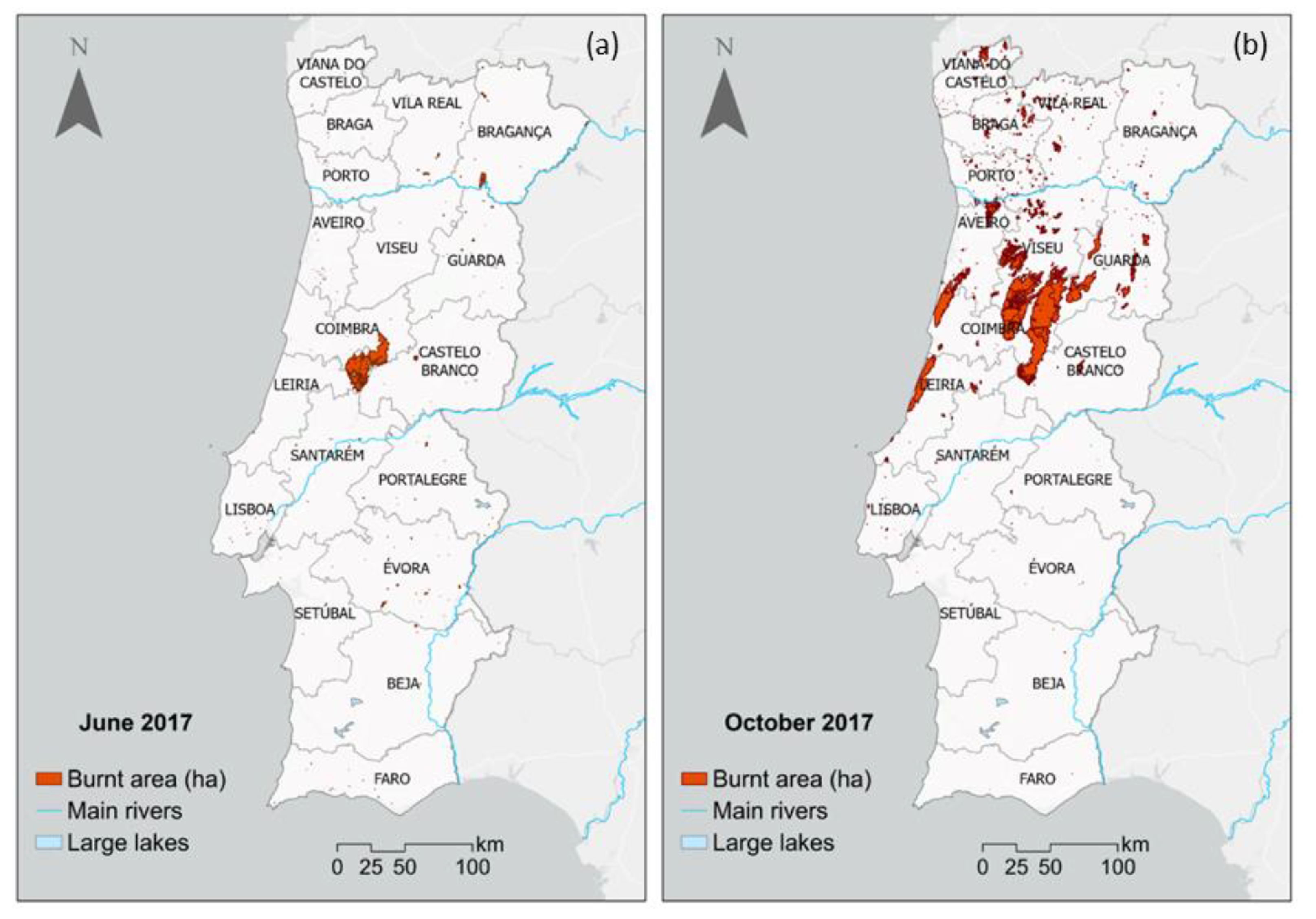
2.1. Study Area

Mainland Portugal is in the southwesternmost portion of Europe in the Iberian Peninsula. Its territory has a total area of about 88,962.5 km² with elevations that vary from 0 m (near the Atlantic Ocean) to 1991 m (in the Serra da Estrela located in the eastern center) and a mean elevation of about 323 m above sea level. Portugal and Spain share three major rivers: the Douro (in the north), the Tagus (in the center), and the Guadiana (in the south). According to Köppen’s climate classification, Portugal has a Mediterranean-like climate (CS). The prominent climate is CSa (warm temperate/Mediterranean with a hot summer) and is mostly found in the southern half of the country and a small region in the northeast [11]. The remainder of the territory, mostly found northwards of the Tagus River basin, has a warm temperate/Mediterranean with a warm summer (CSb).

Average annual temperatures in mainland Portugal range from 18 °C in the south to 10 °C in the inner center. Annual rainfall varies from less than 500 mm in the southernmost regions to over 3000 mm in the north. The country’s coldest location is in Serra da Estrela, which has an average annual temperature of 7 °C at the highest altitudes. Overall, the precipitation regime in Portugal presents great interannual variability.

Portugal’s capital is Lisbon, located in the center of the country near the coast and the Tagus River. Lisbon is the major metropolitan area of the country, with about 2,871,133 inhabitants. The population distribution within Portugal reveals high contrasts between the more densely populated regions in the north near the coast and the more sparsely populated regions in the southern and inner regions. With their low-lying plains and urban development, the coastal zones between Oporto and Lisbon have attracted a large percentage of the Portuguese population. This fact has resulted in the depopulation of the inner regions, which are characterized by an aged population and abandoned agriculture and forest areas.

Portugal’s vegetation is a mixture of Atlantic/European and Mediterranean species. The south (the Alentejo region) is characterized by extensive areas of matorral, charneca, and uncultivated land dominated by cistus (Cistus ladanifer), olive trees (Olea europaea), cork oak (Quercus suber), and holm oak (Quercus ilex). In its southernmost portion (the Algarve region), vines and groves of Mediterranean trees such as olives, citrus (Citrus sps), figs (Ficus carica), almonds (Prunus dulcis), and carob (Ceratonia siliqua) are dominant. The thickest forests are in the inner center, in which pines (genus Pinus), chestnut groves (Castanea), and oak trees (Quercus robur) are found, along with ericas (genus Erica) in the dense maquis. It is worth mentioning that in this region, the elevation succession of vegetation is strongly marked on the Serra da Estrela. In the Douro valley (in the northeast), juniper scrub has been replaced by vineyards. Overall, mixed deciduous trees are prominent in the north and inner north regions, and the remaining part of the country features two types of Mediterranean scrublands: maquis and matorral or steppe. The original oak trees (Quercus robur) have been largely replaced by pine (genus Pinus), cork oak (Quercus suber), and extensive plantations of eucalyptus (genus Eucalyptus).

The study area is within the geographical sector: 36.935° N–42.105° N and 9.515° W–6.105° W. However, all figures presented herein will be clipped, excluding the grid boxes over the Atlantic Ocean.

2.2. Indices Description

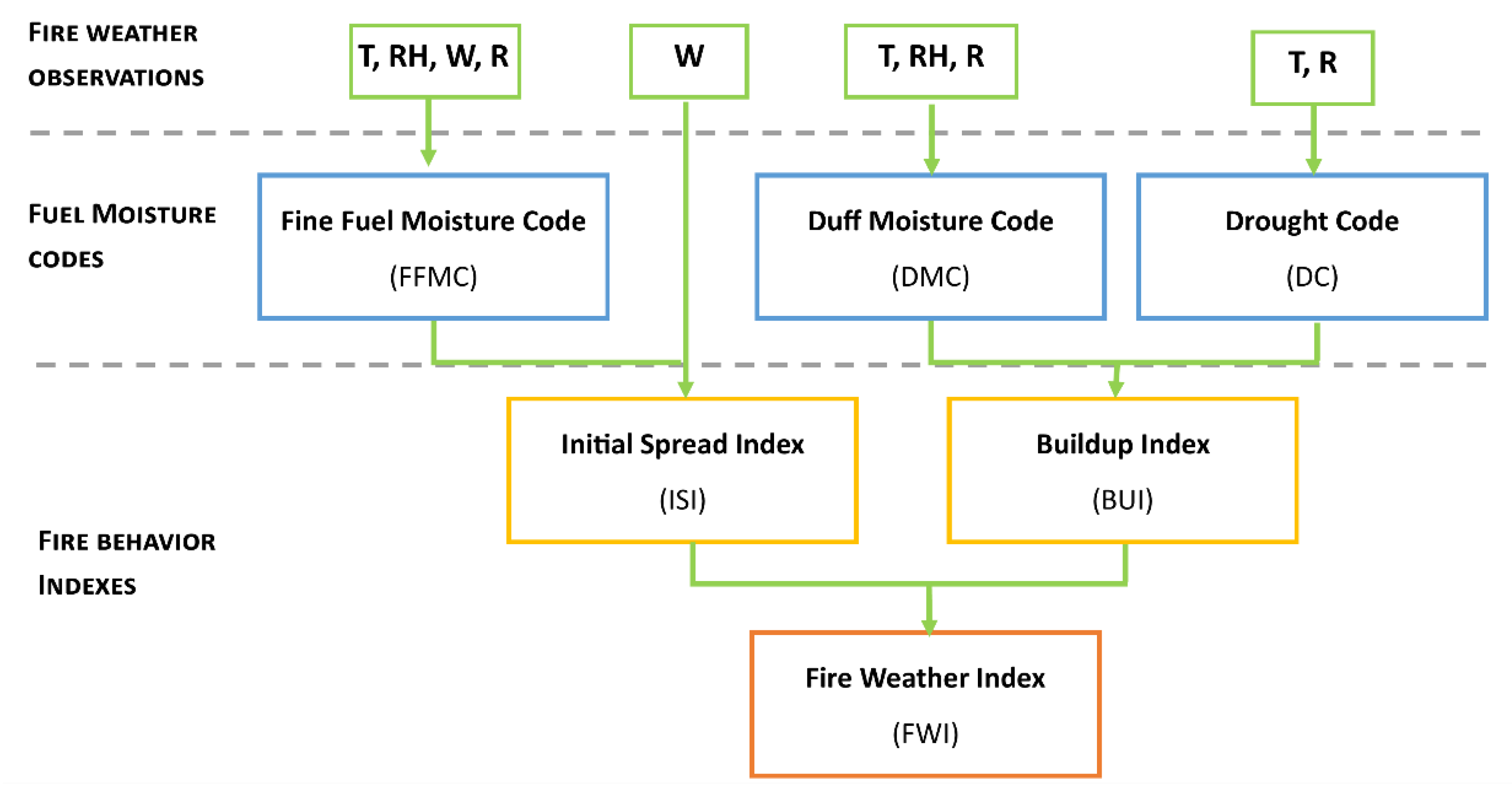
2.2.1. The Fire Weather Index (FWI)

The FWI was developed by the Canadian Forest Service and is a combination of four weather observational variables (air temperature, relative humidity, wind, and rain) that recursively give rise to a set of three fuel moisture codes: the fine fuel moisture code (FFMC), the Duff moisture code (DMC) and the drought code (DC) (Figure A2 for further details); which in turn are used to compute two fire behavior indices: ISI computed from FFMC, and wind and BUI computed from DMC and DC (Figure A2). With these latter indices (ISI and BUI), the FWI is finally attained for a certain day [31,47] to produce a general fire intensity potential (Figure A2).

The FWI scale is shown in

Table 1. Fire Weather Index (FWI) scale and interpretation.

FWI	Color Code	Interpretation
0–8.5	Green	Very low
8.5–17.3	Yellow	Low
17.3–24.7	Light orange	Moderate
24.7–38.3	Orange	High
38.3–50.1	Red	Very high
50.1–64	Dark red	Extreme/Maximum
>64	Brown

, which for Portugal classifies regions with FWI values higher than 38.3 as regions of extreme danger [48]. This class, FWI > 38.3, is further subdivided into three classes: between 38.3 and 50.1, between 50.1 and 64, and FWI values above 64 ([36], accessed on 01 February 2022). It is worth emphasizing that this subdivision was due to the large fires of 2017, in which the values achieved for the FWI were much higher than the average value expected for the region and period (June and October) of occurrence.

2.2.2. The Continuous Haines Index (CHI)

In this study, the daily values of CHI were computed and analyzed. This index is a predictor of atmospheric instability and, thus, high CHI values are indicators of a very unstable atmosphere, with high dryness, supportive of strong convection. This indicates the potential for fires to become larger or erratic, as vertical movement of air can give rise to strong convection columns above a fire with strong indraft winds at ground level as a result. Overall, an unstable atmosphere will promote convection and assist in escalating fire behavior.

When comparing CHI with the Haines Index (HI) [30,44,49], CHI eliminates the abrupt transitions between categories and provides major contrast at higher values. Furthermore, it allows a more realistic assessment of the contributions of atmospheric instability and dew point depression to the overall score [50]. The CHI is also a combination of two terms, a continuous stability term, ca, and a continuous moisture term, cb, and is computed by following Equations (1)–(3):

ca = 0.5 (T850 − T700) − 2,

(1)

cb = 0.3333 (T850 − DP850) − 1,

(2)

CHI = ca + cb,

(3)

in which, T700 and T850 are the air temperatures (°C) at 700 hPa and 850 hPa, respectively; and DP850 is the dew point temperature (°C) at 850 hPa. Regarding the classification scale, the main difference between HI and CHI is that CHI ranges from 0 to 14 (

Table 2. Continuous Haines index (CHI) scale and interpretation.

CHI	Probable Fire Behavior and Fire Prediction Reliability
<4	Easily controlled fire. Models easily predict the path of the fire.
4–8	Fires can be difficult to control, and their behavior can be erratic. The modeling of the behavior of the fire is likely to be close to reality.
8–10	Fires will be difficult to control, and the behavior of the fire will be erratic. Modeling the behavior of the fire likely underestimates reality.
>10	Fires are uncontrollable and extremely difficult to extinguish. Modeling of fire behavior dramatically underestimates reality.

) since ca and cb have upper limits of approximately 6.5 and 7, respectively.

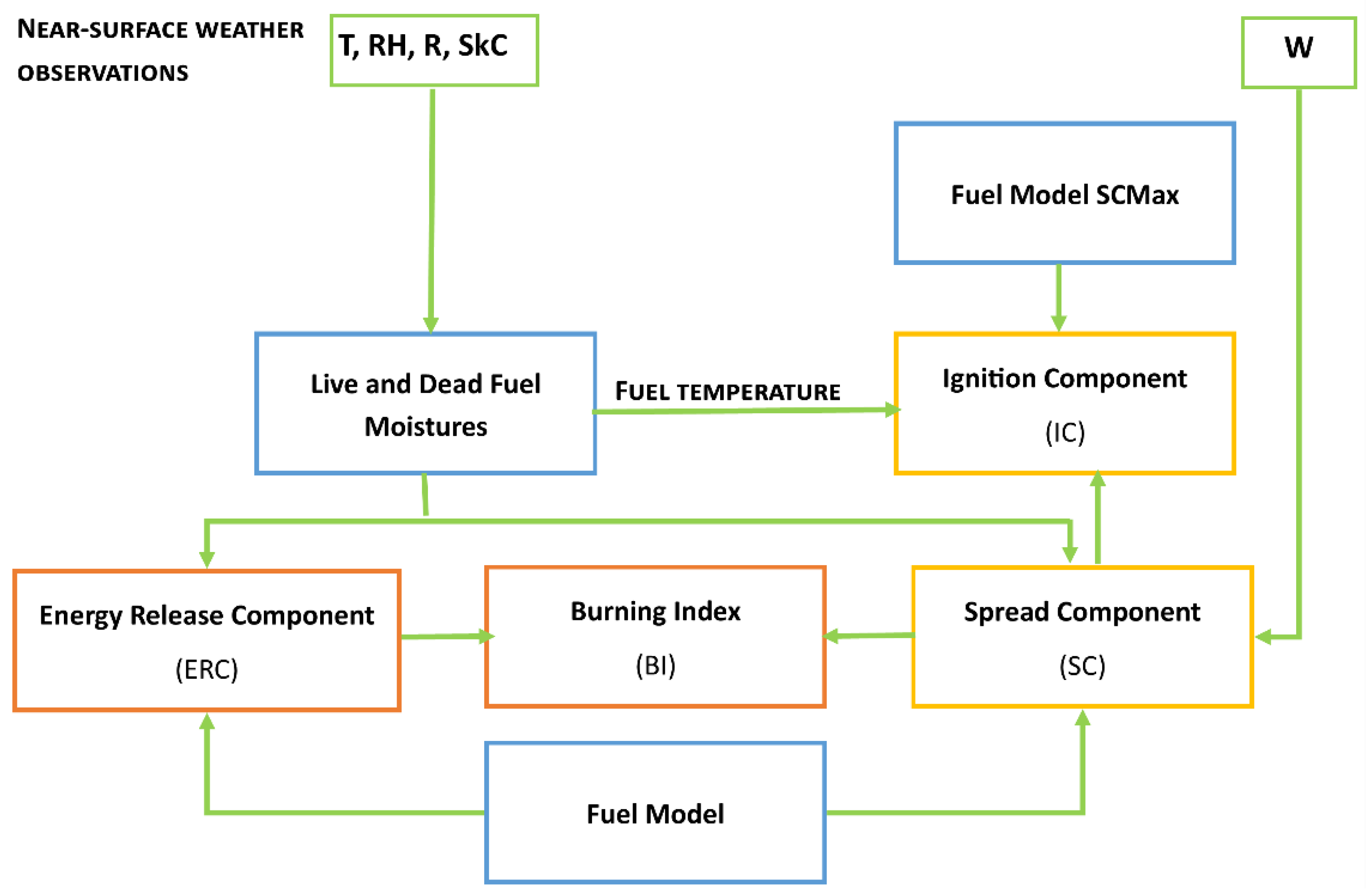
2.2.3. NFDRS: Burning Index (BI), Energy Release Component (ERC), Spread Component (SC), and Ignition Component (IC)

FWI and CHI are not the only indices that allow us to assess the conditions prone to the occurrence of wildfires. As mentioned above, the NFDRS also provides several indices, such as the BI, that are analogous to FWI (Figure A3). Like FWI, BI integrates the SC (how fast a fire will spread) and the energy release component (ERC, how much energy will be produced). Therefore, BI is a function of a fuel model (e.g., live and dead fuel moistures) and weather conditions. Following the instructions of the U.S. Forest Service regarding fire behavior and its suppression, the BI can be interpreted as in

Table 3. Burning index (BI) scale and interpretation (adapted from the traditional U.S. Forest Service interpretation of the Burning Index [38]).

BI	Fire Behavior and Suppression
<40	Fires can be attacked at the head or flanks by firefighters using hand tools. The hand line should hold the fire.
40–80	Fires are too intense for a direct attack on the head by firefighters using hand tools. The hand line cannot be relied on to hold fire. Equipment such as dozers, pumpers, and retardant aircraft can be more effective.
80–110	Fires may present serious control problems torching out, crowning, and spotting. Control efforts at the fire head will probably be ineffective.
>110	Crowning, spotting, and major fire runs are probable. Control efforts at the head of the fire are ineffective.

, which has a similar correlation with the scale presented in Table 1 for FWI, mainly in the first three classes, since it will give a number related to the contribution of fire behavior to the effort of containing it.

The BI is computed by:

$${\mathrm{F}}_{\mathrm{L}}=\mathrm{j}{\left[\left(\frac{\mathrm{SC}}{60}\right)25\times \mathrm{ERC}\right]}^{0.46},$$

(4)

where j is a scaling factor and ERC is the Energy Release Component; hence:

$$\mathrm{BI}={\mathrm{j}}_1{\mathrm{F}}_{\mathrm{L}},$$

(5)

in which ${\mathrm{j}}_1$ is the scaling factor of (10/ft).

Regarding the SC, this variable is a measure of the speed at which the head fire will spread and is numerically equal to the theoretical ideal rate of spread per foot. However, it is considered a dimensionless variable.

The IC is also going to be analyzed and measures the probability (which ranges from 0 to 100%) of a firebrand requiring a suppression action. The higher the IC values, the higher the probability of a wildfire requiring suppression actions. Consequently, an IC of 100% implies that every firebrand will trigger a fire that will require action when in contact with a receptive fuel. Conversely, an IC of 0% indicates a firebrand that will not require fire suppression action under those conditions.

2.2.4. The Keetch–Byram Drought Index (KBDI)

The KBDI is also encompassed in the NFDRS indices and represents the net effect of evapotranspiration and precipitation in producing cumulative moisture deficiency in deep duff and upper soil layers. Like BUI, the KBDI is a continuous index, linked to the flammability of organic material in the ground and attempts to measure the amount of precipitation necessary for the soil to return to saturated conditions. Therefore, KBDI was designed as a drought index to assess fire potential [40,51] and is like the FWI’s DC. As such, it represents the net evapotranspiration and precipitation in producing cumulative moisture deficiency in deep duff and upper soil layers. It is a closed system ranging from 0 to 200 units and represents a moisture regime of 0 to 20 cm of water through the soil layer. At 0, KBDI assumes the point of no moisture deficiency, at 20 cm of water, assumes saturation, and at 200 assumes the maximum drought that is possible to occur. Therefore, at any point along the scale listed in

Table 4. Keetch–-Byram drought index (KBDI) scale and interpretation (adapted from the traditional U.S. Forest Service interpretation of the Keetch–Byram drought index [38]).

KBDI	Fire Behavior and Suppression
0–50	Soil moisture and large-class fuel moistures are high and do not contribute much to fire intensity. Typical of the spring dormant season following winter precipitation.
50–100	Typical of late spring, early growing season. Lower litter and duff layers are drying and beginning to contribute to fire intensity.
100–150	Typical of late summer, or early fall. Lower litter and duff layers actively contribute to fire intensity and will burn.
150–200	Often associated with more severe drought with increased wildfire occurrence. Intense, deep-burning fires with significant downwind spotting can be expected. Live fuels can also be expected to burn actively at these levels.

, the index number indicates the amount of net rainfall that is required to reduce the index to zero, or saturation.

2.2.5. The Forest Fire Danger Index (FFDI)

The FFDI is integrated within the Australian McArthur Mark5 Rating System and is an index associated with the danger conditions prone to a fire starting, its rate of spread, its intensity, and the difficulty in its suppression. Like other preferred indices, it is open-ended though a value equal to or above 50 is considered indicative of the extreme danger of wildfire in most vegetation. It is worth mentioning that in this study the scale used was adopted from Luke and MacArthur [51], though Wain and Kepert [52] had proposed a new fire danger rating for bushfires in 2013: 0–12 Low-Moderate, 12–24 High, 24–50 Very High, 50–75 Severe, 75–100, and Catastrophic above 100. The FFDI is attained by

$$\mathrm{FFDI}=2{\mathrm{e}}^{\left(-0.45+0.987\ln \left(\mathrm{DF}\right)-0.0345\mathrm{RH}+0.0338\mathrm{T}+0.0234\mathrm{v}\right)},$$

(6)

where DF is a drought factor, T is the air temperature (°C), RH is the relative humidity (%), and v is the wind speed (km/h) (consult Luke and MacArthur [51] for further details).

2.3. Datasets

This study comprises a study area covering mainland Portugal for all indices and the 2001–2021 period. The interval includes an extremely high 2017 fire year in terms of burned area, although 2003 and 2005 also have record values; as well as an extremely low 2007, even though 2008 could be also considered (Figure A1) ([53], accessed on 1 February 2022). Individual fire data, such as date, duration, location, and size were retrieved from ICNF, the Portuguese rural fire database ([43,53,54,55], accessed on 31 November 2021). In this study, all data regarding the burned areas between 2001–2021, but mainly during the days covering the great CEWEs of 17 June 2017, and 15 October 2017, were all retrieved from ICNF ([43], accessed on 31 November 2021). For succinctness, the analysis is focused on the months most prone to the occurrence of wildfires in Portugal, e.g., between May and October for all indices, thus encompassing the fire season.

For the CHI computation, Matlab routines were written. To attain CHI, daily datasets of the air temperature (at 700 hPa and 850 hPa, in °C) and the relative humidity (%) at 850 hPa [30,44,49] were retrieved from the European Centre for Medium-Range Weather Forecasts (ECMWF) atmospheric model between 2001 and 2021 ([56], accessed on 13 January 2022) at 12UTC on a 0.125° × 0.125° latitude-longitude regular grid.

The FWI and its sub-indices were computed by using daily values at 12UTC on a 0.125° × 0.125° regular grid of air temperature (at 2 m in °C), and relative humidity (at 2 m in %) attained from the dew point temperature (in °C). Wind speed (at 10 m in m/s) was computed from the zonal and meridional components. Lastly, the accumulated total precipitation (in mm) was calculated from convective rain and large-scale rain all retrieved from the ECMWF atmospheric model ([56], accessed on 13 January 2022), also between 2001 and 2021. All FWI computations were performed by using IPMA’s FORTRAN90 routines that follow Van Wagner and Picket [31] codes. These routines were also translated into Matlab routines to perform further statistical analysis.

The remaining daily values for BI, SC, ERC, IC, KBDI, and FFDI for the studied area and periods were retrieved from Copernicus datasets ([57], accessed on 3 January 2022).

2.4. Statistical Analysis

The period 2001–2021 between May and October, was considered a ‘baseline climate’ or reference/control period. The Student’s t-test (TST) was applied to the monthly average values between the reference period, 2017 and 2007 for FWI, CHI, KBDI, BI, and FFDI mean values at a 5% significance level. This test returns a decision for the null hypothesis (H_o = 0) which assumes that the two series are from populations with equal means, against the alternative hypothesis (H_a = 1) of having different means. These results will be presented in Section 3.1.

In climatological studies, an anomaly is defined as the difference between a certain period and a baseline climate (or reference period) for a given variable. In this study, monthly anomalies (or differences) were computed by subtracting 2017 from the related data for the reference period for FWI, CHI, FFDI, BI, and KBDI within the study area. The statistically significant anomalies (S.S.) were then assessed by applying the Mann–Whitney–Wilcoxon test (MWW), at a 5% significance level [58,59] for each month and location (i.e., point-by-point) of the study area. This nonparametric test assumes equal medians under the null hypothesis (H_o), against the alternative hypothesis (H_a) of different medians. These results will also be presented in Section 3.1.

Finally, a hotspot analysis was performed for both the burned areas of 17 June and 15 October 2017, for all variables (excluding KBDI and BUI). The hotspot analysis is a spatial analysis and mapping technique that identifies clusters of spatial phenomena. These locations are depicted as points on a map and refer to the locations of events or objects. Overall, this technique identifies statistically significant spatial clusters of high/low values (hot/cold spots), e.g., high/low concentration of events compared to the expected number given a random distribution of events. There are different methods for analyzing spatial patterns and detecting hotspots, including spatial autocorrelation and cluster analysis. The nearest neighbor index, which is an indicator for clustering, compares the observed distribution of events against an expected random distribution of these values. The significance of the difference between the observed and the random expectation is tested using a Z-score. Spatial autocorrelation assesses how similar the values that are closer to each other are. The application of hotspot analysis has increased significantly due to the advent of geographic information system-based software [60,61]. In this case, ArcGIS Pro tools were used. In this study, this technique was applied to aim at identifying the clustering of spatial phenomena, thus statistically defining areas of high or low occurrences between the previously mentioned indices and the burned areas. These results will also be presented in Section 3.3.

2.5. Methodological Framework

The methodological framework of this study can be depicted in Figure 1.

Figure 1. The methodological framework of this study.

Figure 1. The methodological framework of this study.

The methodological procedures were divided into two distinct timeframes a monthly mean analysis (first phase in Figure 1) and a daily mean analysis (second phase in Figure 1). Therefore, the results section was divided into three main subsections. In the first, Section 3.1, an assessment of the monthly maximum and mean average values between May and October for FWI, CHI, FFDI, BI, and KBDI, between 2001 and 2021, is presented. Since the main aim of this subsection is to perform a climatological assessment of the behavior of the main indices, only the months comprising the fire season were analyzed. As such, the short-term variation sub-indices of the FWI and BI were not included. A comparison between the reference period and 2017 (extremely high occurrence of wildfires) and 2007 (extremely low occurrence of wildfires) are also undertaken. In this subsection, the results of two statistical tests previously described in Section 2.4 are presented.

In the second, Section 3.2, the assessment of the indices’ spatial distribution is performed daily, namely, between 16 and 20 June and between 14 and 16 October 2017. In this subsection, the impact of the meteorological conditions on the scale and spatial distribution can be inferred. Within these periods, the most catastrophic fire events (in terms of the total burned area and human fatalities) occurred on 17 June (commonly known as the Pedrógão Grande wildfire) and 15 October 2017 (

Table 5. List of the total burned areas (ha) by the district on 17 June and 15 October 2017 (only the major wildfires were considered) ([53,54] accessed on 1 February 2022).

Date	District	Urban Areas (ha)	Bush Areas (ha)	Total Burnt Area (ha)
17 June 2017	Leiria	30,359.00	0.15	30,359.18
	Coimbra	9483.30	8037.64	17,521.45
				47,880.63
15 October 2017	Coimbra	89,638.08	11,014.75	11,1582.20
	Guarda Castelo Branco	24,836.50 21,290.01	17,664.23 12,991.67	47,649.22 35,790.34
	Leiria	19,283.93	984.40	20,741.06
	Viseu	11,969.01	4623.15	18,013.13
	Aveiro	8787.08	1875.89	11,421.33
				245,197.30

and Figure 2). The total burned area during these two days in the case of October has affected a vast number of urban areas. The total burned area was greater than 300 kha (Table 5; Figure A1) and was concentrated in the Coimbra, Guarda, Castelo Branco, Leiria, Viseu, and Aveiro districts in the center of Portugal (Figure 2).

This daily analysis is going to be divided into five sub-sections, as follows:

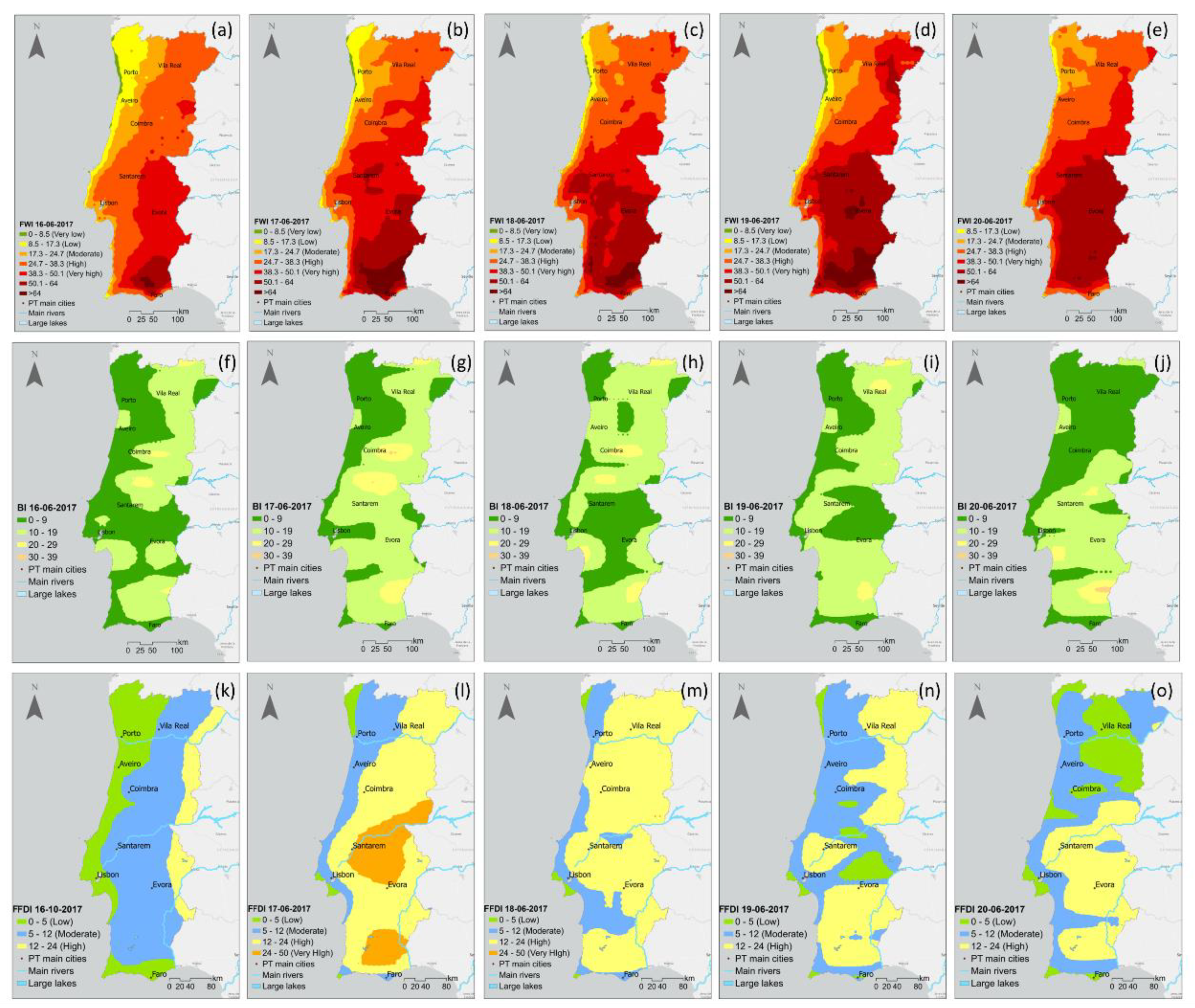
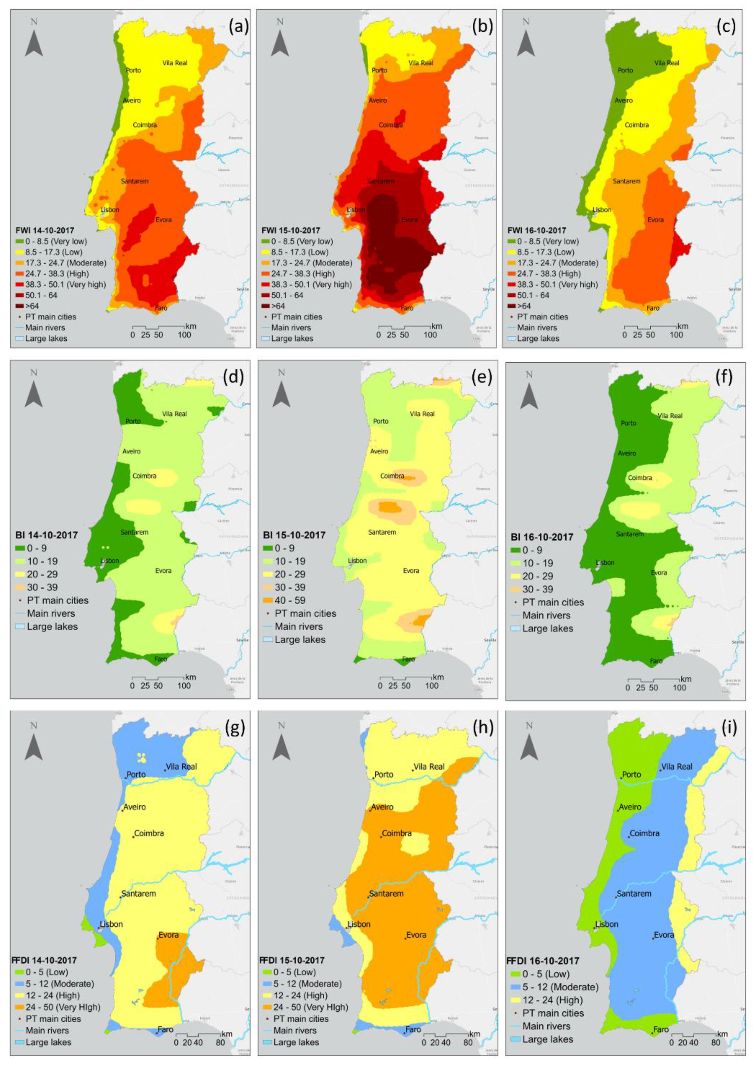
• in Section 3.2.1, a comparison between the spatial patterns of FWI, BI, and FFDI is presented. These indices are associated with fire intensity.
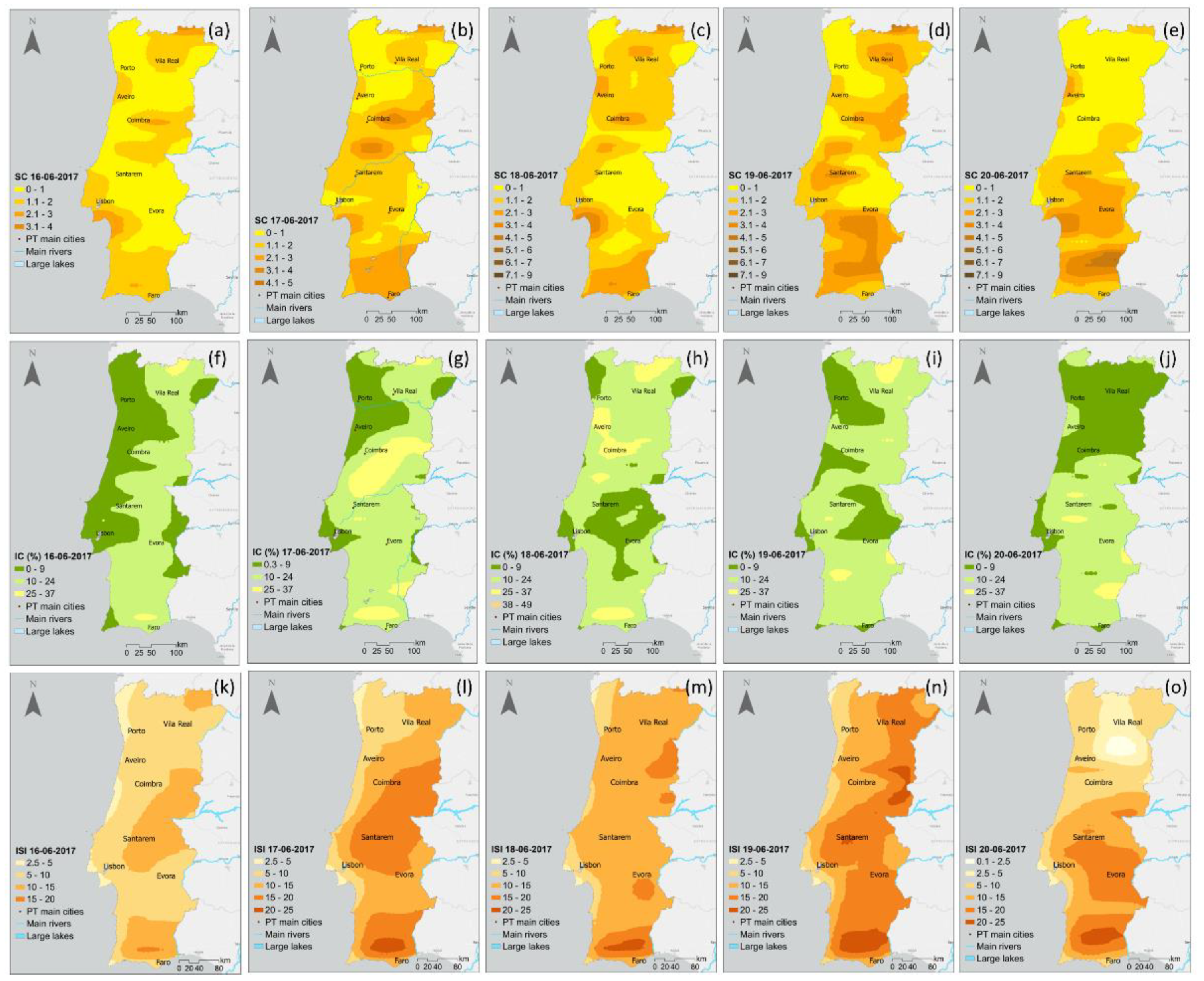
• in Section 3.2.2, the spatial patterns are presented and compared for the components with a daily scale variation, i.e., SC, ISI, associated with the spread of fires and IC with their ignition.
• in the next two sections, the indices with longer variation timescales

  o

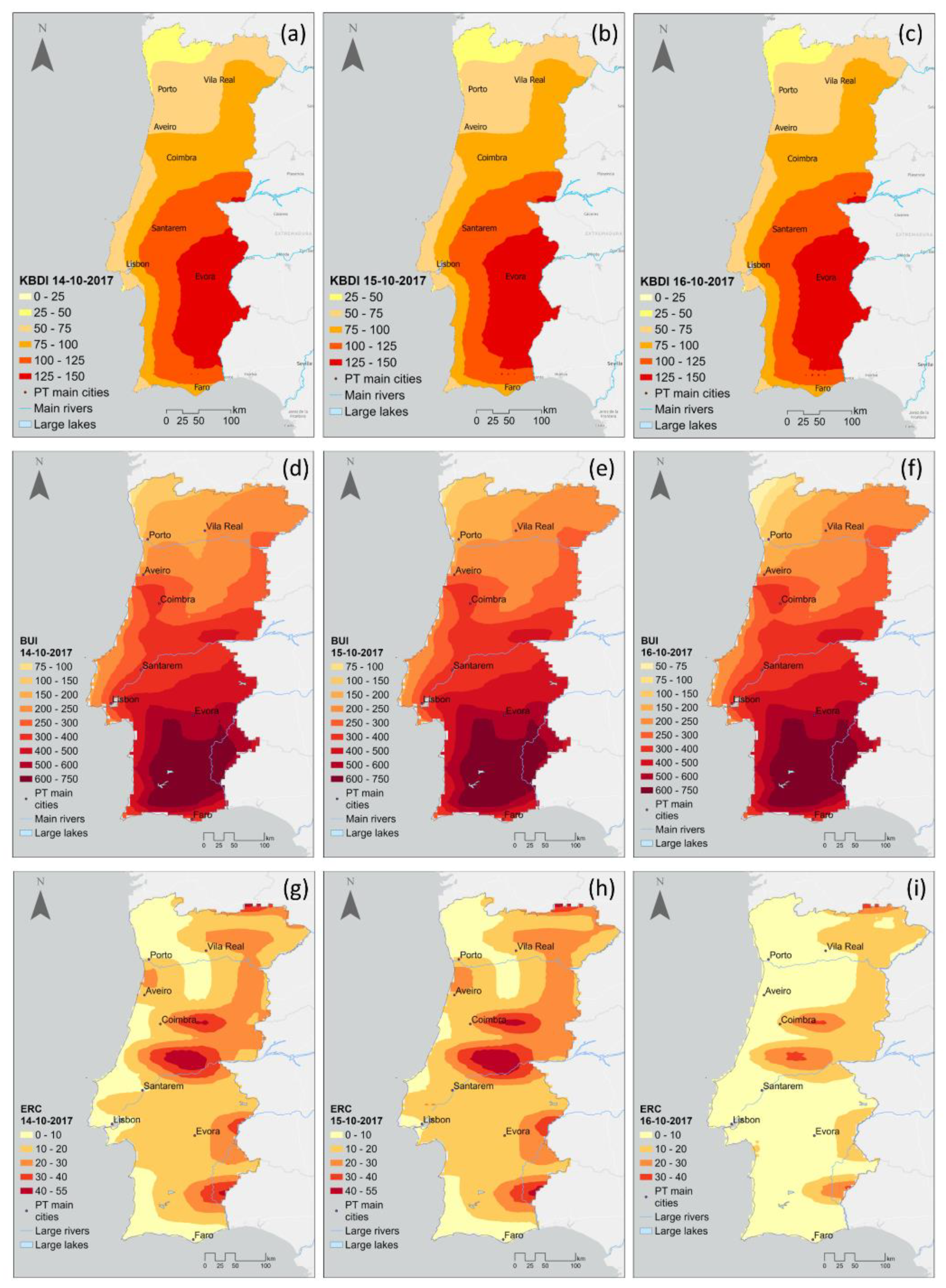
  Section 3.2.3 KBDI which is associated with drought conditions.

  o

  Section 3.2.4 BUI and ERC linked to fuel weight availability to the flame front are analyzed.

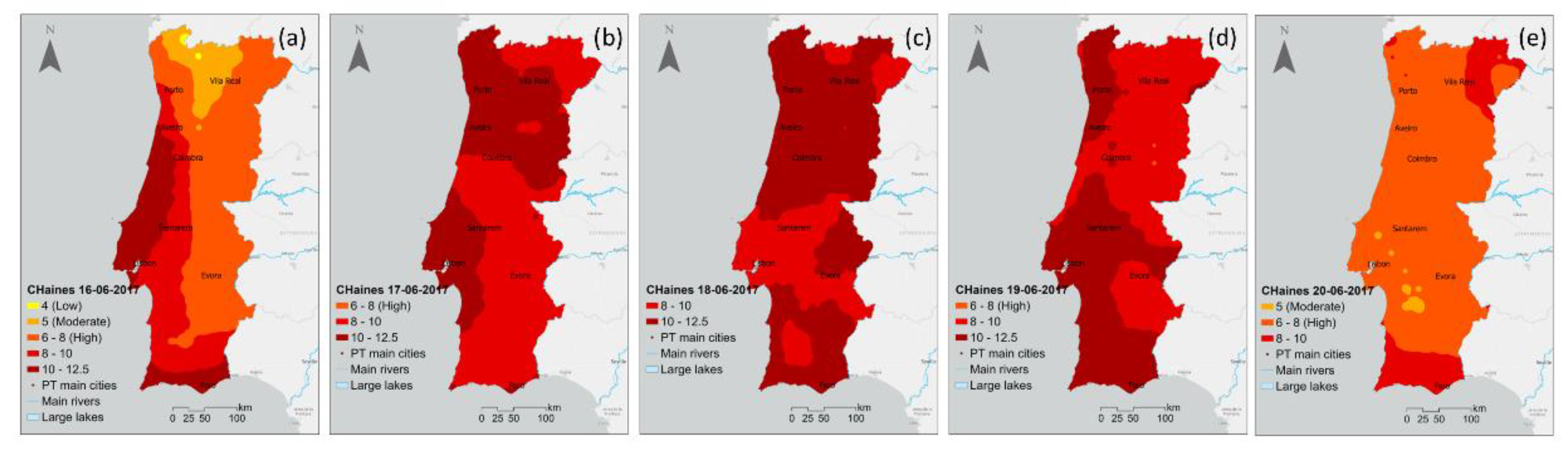
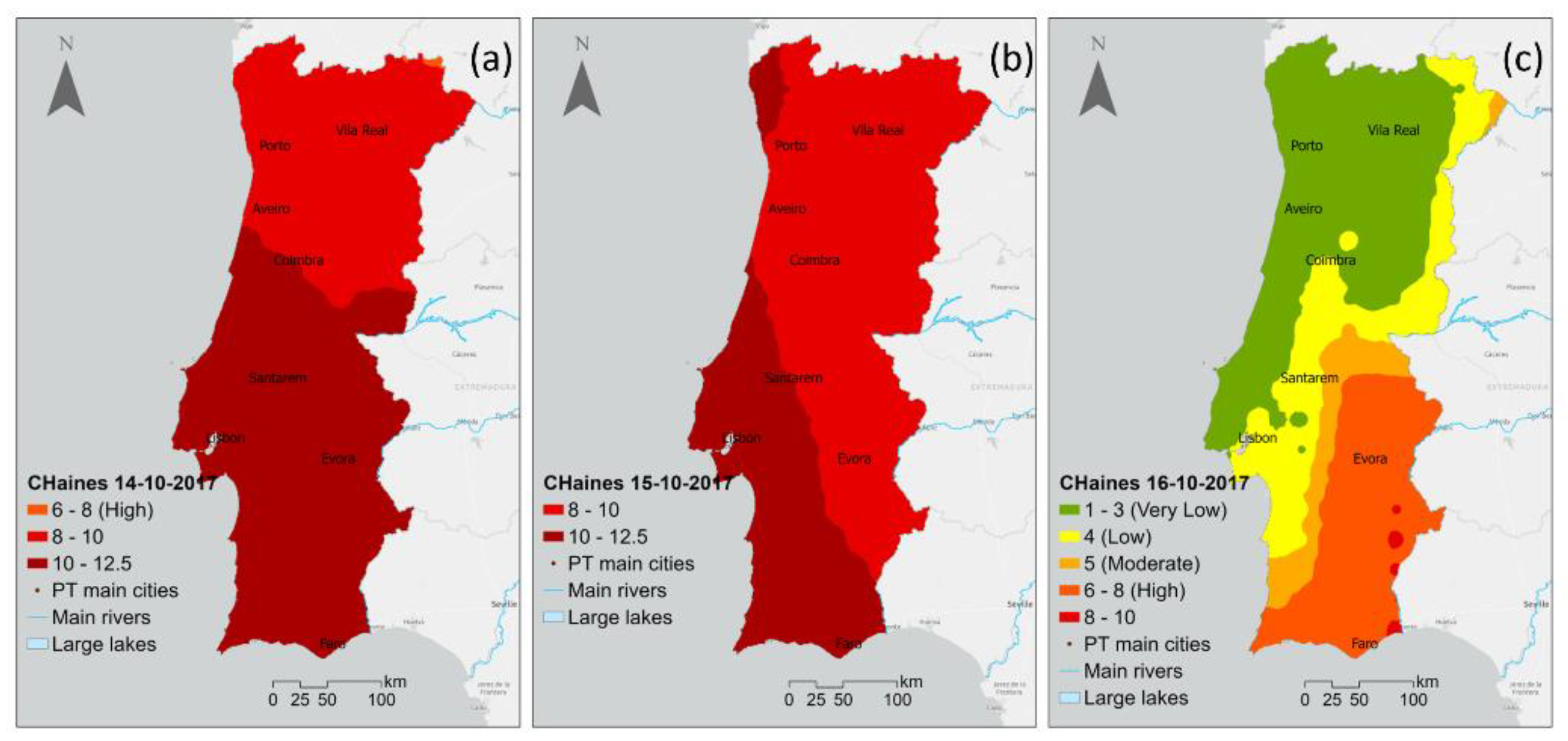
• in Section 3.2.5, the CHI daily spatial patterns for the two CEWEs are also shown. This index is related to the vertical atmospheric conditions.

Lastly, the results Section 3.3 ends with the outcomes attained from a hotspot analysis performed between some of these indices and the burned areas for 17 June and 15 October 2021. This assessment allows us to identify the association between the statistically significant spatial patterns of the clusters of the indices (hot/cold hotspots) with the burned areas.

3. Results

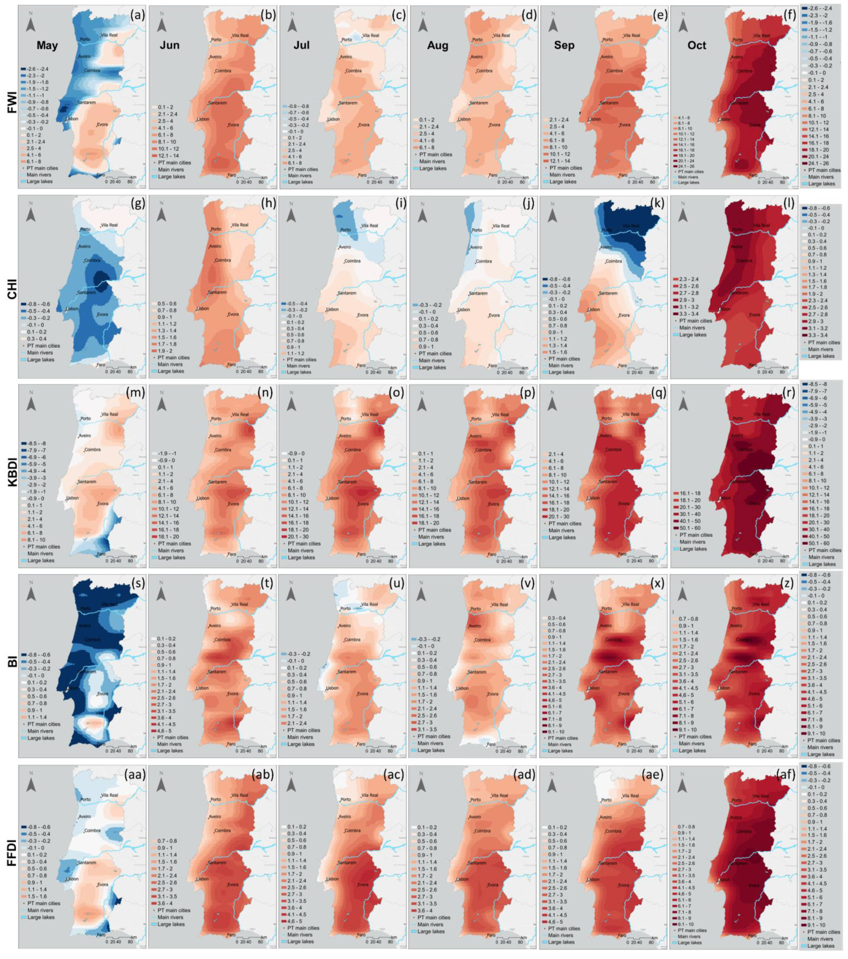
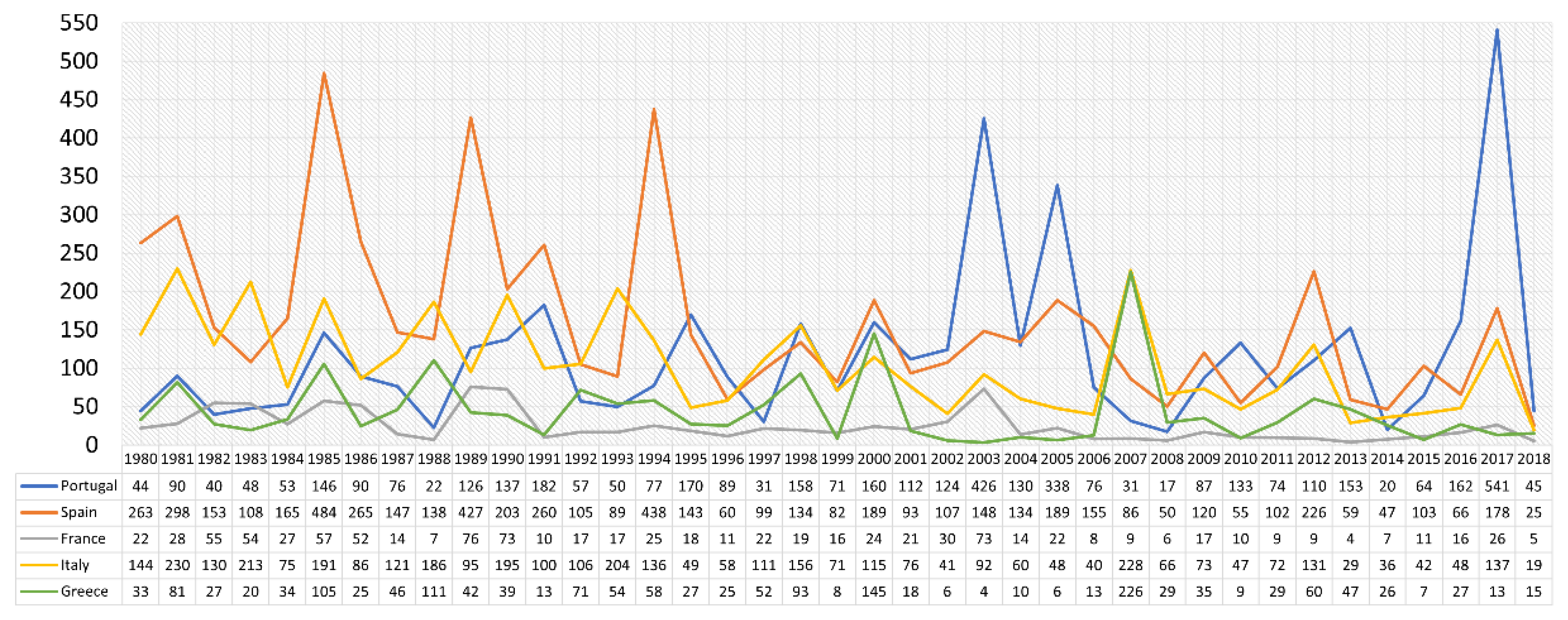
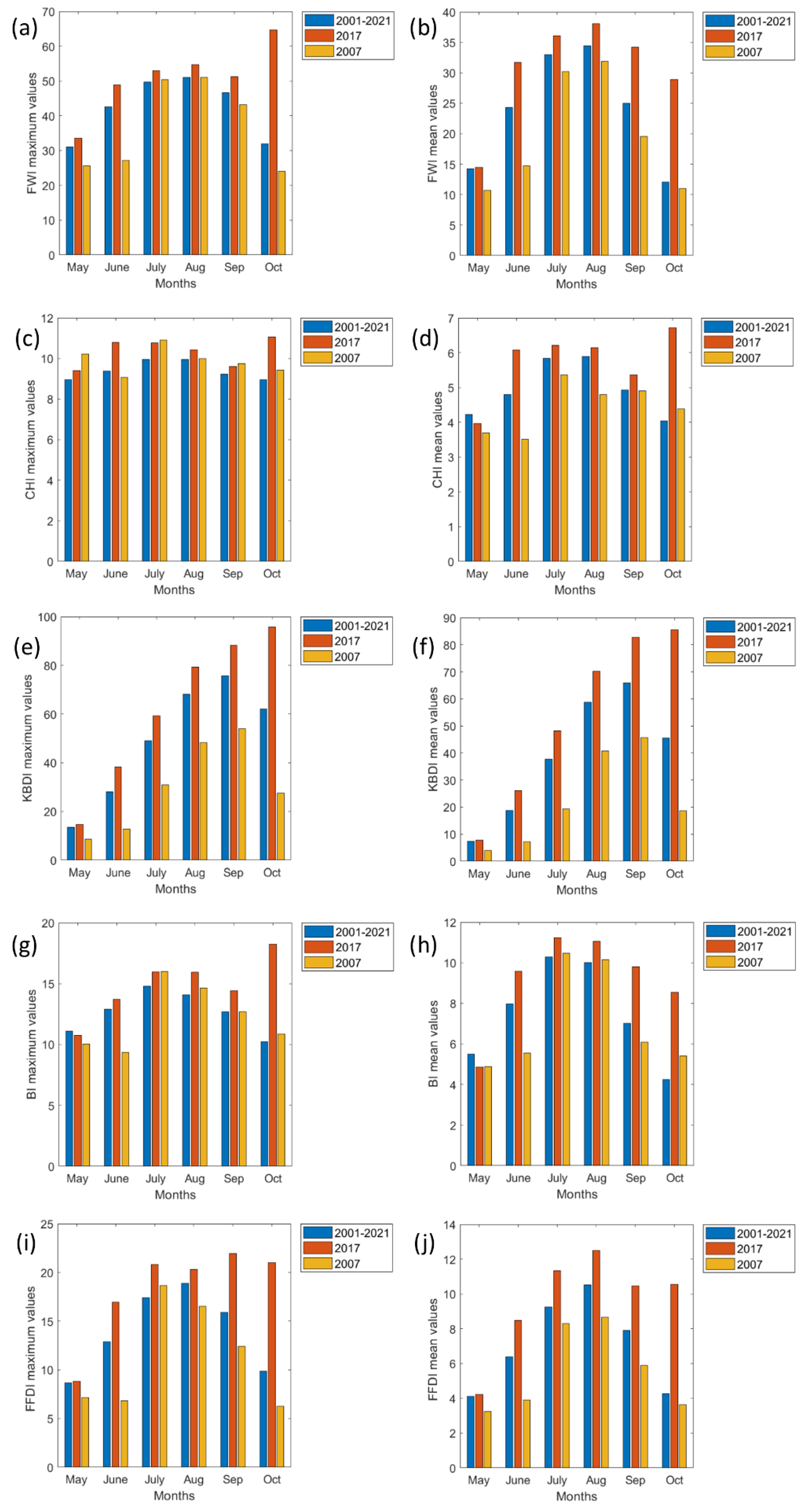
3.1. Monthly Mean Analysis

A comparison between the reference period and 2017 (with an extremely high maximum value of burned area) and 2007 (extremely low value of burned area) for the main indices FWI, CHI, KBDI, BI, and FFDI was performed. For both the maximum and mean monthly average values (Figure A1 and Figure A4;

Table 6. Maximum and mean monthly average values for 2001–2021 (baseline climate), 2017, and 2007 for FWI, CHI, KBDI, BI, and FFDI, respectively for mainland Portugal.

	2001–2021	2017	2007	2001–2021	2017	2007
	Maximum FWI			Mean FWI
May	31.1	33.6	25.6	14.3	14.5	10.7
Jun	42.5	48.9	27.3	24.3	31.8	14.7
Jul	49.7	53.1	50.3	33.0	36.1	30.2
Aug	51.0	54.7	51.0	34.4	38.1	31.9
Sep	46.6	51.2	43.2	25.0	34.2	19.6
Oct	32.0	64.7	24.0	12.0	28.9	11.0
	Maximum CHI			Mean CHI
May	8.9	9.4	10.2	4.2	4.0	3.7
Jun	9.4	10.8	9.1	4.8	6.1	3.5
Jul	10.0	10.8	10.9	5.8	6.2	5.4
Aug	9.9	10.4	10.0	5.9	6.1	4.8
Sep	9.2	9.6	9.7	4.9	5.4	4.9
Oct	9.0	11.1	11.1	4.0	6.7	4.4
	Maximum KBDI			Mean KBDI
May	13.6	14.7	8.5	7.4	7.7	4.0
Jun	28.2	38.3	12.7	18.8	26.1	7.2
Jul	49.0	59.3	30.9	37.7	48.3	19.3
Aug	68.2	79.2	48.3	58.7	70.3	40.8
Sep	75.7	88.1	54.0	65.9	82.7	45.7
Oct	62.2	95.8	27.4	45.5	85.5	18.6
	Maximum BI			Mean BI
May	11.1	10.8	10.0	5.5	4.9	4.9
Jun	12.9	13.7	9.3	8.0	9.6	5.6
Jul	14.8	16.0	16.0	10.3	11.2	10.5
Aug	14.1	15.9	14.7	10.0	11.1	10.1
Sep	12.7	14.4	12.7	7.0	9.8	6.1
Oct	10.2	18.2	10.9	4.3	8.5	5.4
	Maximum FFDI			Mean FFDI
May	8.7	8.8	7.1	4.1	4.2	3.2
Jun	12.9	16.9	6.8	6.4	8.5	3.9
Jul	17.4	20.8	18.6	9.3	11.3	8.3
Aug	18.9	20.3	16.5	10.5	12.5	8.7
Sep	15.9	21.9	12.4	7.9	10.5	5.9
Oct	9.8	21.0	6.3	4.3	10.6	3.7

), anomalous conditions for 2017 are depicted. The Student’s t-test at a 5% S.L. was applied between the reference period, 2017 and 2007, and the p-values are shown in

Table 7. Student’s t-test p-values (at a 5% significance level) for the monthly average values between 2001–2021, 2017, and 2007 for FWI, CHI. KBDI, BI, and FFDI mean values, respectively for mainland Portugal (H₀ not rejected in bold).

p-Values	FWI		CHI		KBDI		BI		FFDI
2001–2021	2017	2007	2017	2007	2017	2007	2017	2007	2017	2007
May	0.715	0.016	0.126	0.792	0.101	0.000	0.952	0.866	0.005	0.006
Jun	0.000	0.000	0.368	0.122	0.000	0.000	0.000	0.000	0.441	0.000
Jul	0.018	0.061	0.281	0.793	0.000	0.000	0.000	0.034	0.002	0.020
Aug	0.016	0.311	0.037	0.005	0.000	0.000	0.000	0.032	0.008	0.000
Sep	0.000	0.011	0.000	0.127	0.000	0.000	0.000	0.883	0.000	0.000
Oct	0.000	0.233	0.115	0.076	0.000	0.000	0.000	0.004	0.099	0.206

. Between July and September, all indices revealed for 2017 statistically significant mean monthly values above those of the reference period (Figure A4; Table 6 and Table 7). For May 2017, the exceptions were observed for FWI, CHI, KBDI, and BI, and for June and October 2017 for CHI and FFDI. This variation was particularly relevant for October for all indices, either for maximum or the mean monthly average values (Figure A4). The variations between 2017 are statistically significant (TST at a 5% S.L.) for October with the reference period for FWI, KBDI, and BI for the mean monthly average values (Figure A4; Table 6 and Table 7).

The FWI maximum values for all periods are within the very high danger class for July, August, and September, and high for June (Figure A4). Regarding May, the danger is moderate for 2007 and high for the remaining period. Lastly, for October, the danger is moderate for 2007, high for 2001–2021, and extreme for 2017 (Table 6). Results show that the FWI mean values, for May/July are within the low/high danger class for all periods (Table 6). For June, within the low danger range for 2007, in the transition between moderate to high danger for the reference period and high danger for 2017. For August 2017, FWI values are in the transition between high to extreme danger, and high for the remaining periods. FWI values for September and 2007 indicate a moderate danger; for 2001–2021, a moderate to high danger; and for 2017, a high danger. Lastly, for October 2017, FWI values show a high danger and a low danger for the remaining periods (Table 6).

Results show noteworthy variations for the maximum monthly average values of CHI for which some months of 2007 (May, July, and September) were higher in comparison with the reference period and 2017 (Figure A4, Table 6 and Table 7). For FFDI, maximum monthly values (Figure A4d, Table 6) are contained in the first three danger classes (low, moderate, and high danger, respectively), whilst for the mean monthly values, except August 2017 (third class), the remaining are in the second, e.g., the high danger class (Figure A4j, Table 6). Lastly, results show that BI is not highly informative, since only one danger class can be depicted for both cases and all months (Figure A4, Table 6).

Overall, results (hereafter, TST performed always at a 5% S.L.) show that the mean monthly average total values for 2017 (from June to October) are statistically significantly higher in comparison with the reference period. Non-statistically significant mean monthly average total values were found for May (FWI, CHI, KBDI, and BI), but also for CHI (June, July, and October) and FFDI (June and October) for 2017 (Table 6). The mean monthly values of the reference period are statistically significant and higher for most of the indices in comparison with the ones observed for 2007. Non-statistically significant results were found mainly for CHI (statistically significant only for August), FWI (statistically significant only for May, June, and September), and BI during May and September (Figure 2 and Figure A4; Table 6). In these cases, there is no statistical evidence to support that the mean monthly average total values of the reference period are distinct in comparison with the ones observed for 2017 and 2007 (Table 6).

Figure 3 shows the spatial patterns of the MWW statistically significant (hereafter always at a 5% S.L.) monthly mean anomalies (defined in Section 2.4 and Section 2.3, respectively) of FWI, CHI, KBDI, BI, and FFDI. Results are in clear accordance with the ones previously described. Major statistically significant positive anomaly values were depicted for October for all indices (Figure 3f–af) because 2017 values were above the average in comparison with the reference period. Conversely, May presents a more heterogeneous spatial distribution with regions with statistically significant positive and negative anomalies, for which BI (Figure 3s) and CHI (Figure 3g) present negative anomalies almost throughout the country. For May, the northwest region is the most concordant among all indices with statistically significant negative anomalies. Moreover, it can also be seen that there is a similarity in the spatial distribution of May statistically significant anomalies between FWI (Figure 3a), KBDI (Figure 3m), BI (Figure 3s), and FFDI (Figure 3aa). For June, except for KBDI (Figure 3n) throughout the country, statistically significant, positive anomalies were found. For CHI (Figure 3h) and BI (Figure 3t), the highest statistically significant positive anomaly is found in a region south of Coimbra (in the vicinity of the great wildfires of 17 June). For the remaining months, results show a spatial distribution heterogeneity with the statistically significant positive anomalies being prominent. However, for July, statistically significant negative anomalies can again be depicted in the northwesternmost region of the country (Figure 3c,i,o,u,ac). It is still worth mentioning that major statistically significant positive BI anomalies for September and October are in the areas where the major October wildfires occurred (Figure 3x,z). Moreover, even though the monthly mean BI spatial patterns are not very informative due to the scale limitations, their anomalies are quite revealing. High statistically significant positive values can be depicted in June, September, and October 2017; in the areas affected by both CEWEs. The maximum positive statistically significant anomaly values were observed in October 2017 (Figure 3z) thus translating to a long-term spatial sensitivity of this index relative to CEWEs. These results show the relevance of using a multi-indices methodology to analyze extreme fire events.

3.2. Daily Mean Analysis

3.2.1. FWI, BI, and FFDI (Fire Intensity Indices)

The FWI index contains information regarding fuel moisture conditions in the FFMC, DMC, and DC codes. Consequently, the drought situation in June and October of 2017, in Portugal, given the values of these components lead to the high values of the FWI, as shown in Figure 4a–e and Figure 5a–c, respectively. The average value of DC (drought-related FWI sub-index) in mainland Portugal in November 2017 was much higher than the average, being the highest value between 1999 and 2017 (not shown). The average value of the FWI in Portugal was 41.2 (below the 90th percentile) on 17 June and 59.2 (above the 90th percentile), the highest value for 2017, on 15 October.

The increase in the danger for all indices from 16 June to 17 June is highlighted. Results revealed that the BI index reached values above 30 on 17 June, the highest value registered in the country on that day, in a region eastward of Coimbra and the Leiria district (Figure 2a and Figure 4f–j).

The spatial patterns of FFDI revealed a fire danger variation quite similar to the one depicted for FWI and BI. A gradual increase in fire danger from 16 June to 17 June was observed (Figure 4k–l), with values ranging between 22 and 31 (high to very high wildfire danger). The highest values were depicted over a vast region covering the inner center and southern areas (Figure 4l). Indeed, the increasing values are coupled with an intensification in the danger of the occurrence of wildfires. This strengthening is observed from the coast towards inland, and the behavior of the FFDI in the southern regions is, as expected, within the high-danger class.

The outcomes showed that the spatial patterns of FFDI reveal again a danger variation quite like FWI, which is in clear accordance with the very high spatial correlations between these indices (98% at a 5% S.L.) for October for the reference period (not shown). From October 14th to October 15th (Figure 5g–h) a gradual increase in FFDI was again observed, with the highest values ranging between 32 to 39 within the very high wildfire danger range. As previously, these maximum values were observed in a major portion of Portugal comprising the complex of wildfires of 15 October (Figure 5h).

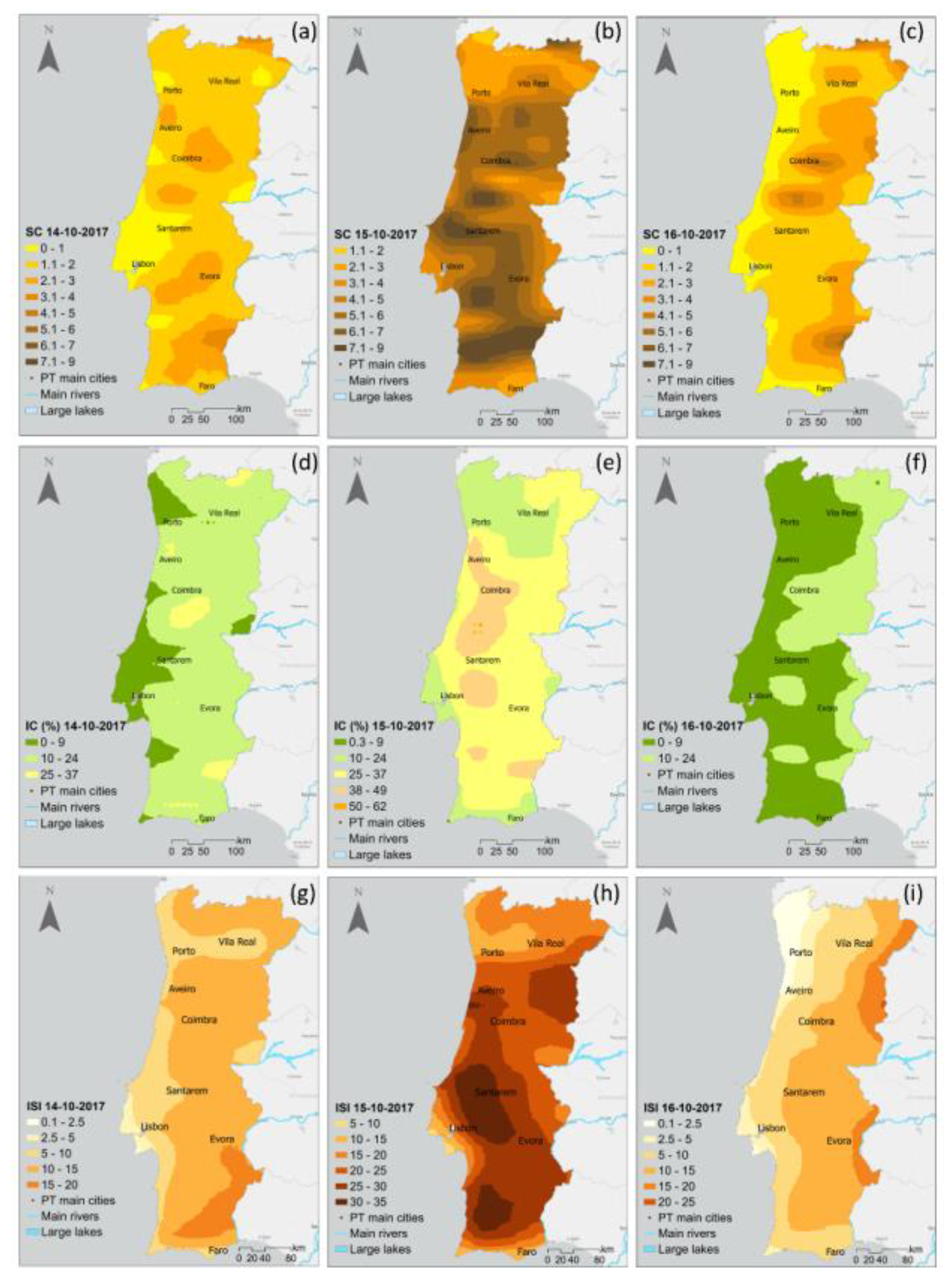
3.2.2. SC, ISI (Fire Spread Related Components), and IC (Fire Ignition Related)

In this subsection, the spatial patterns of SC, ISI (fire spread related components), and IC (related to fire ignition), indices associated with a daily timescale variation (e.g., highly variable mainly due to wind conditions), are going to be analyzed. All indices presented a positive variation towards higher danger values from 16 to 17 June. For SC, IC, and ISI (Figure A5) results show an increase in the central region of Portugal, with the highest values encompassing the region affected by the CEWE of June. It can also be concluded that these indices seem to be able to provide additional information that can be useful to identify regions associated with a high danger for the occurrence of rural fires.

The outcomes revealed that the SC/ISI values have substantially increased in the central region of Portugal (associated with fire spread), again eastwards of Coimbra and in the Leiria district, with the highest values observed on 18/19 June (Figure A5d–n). The IC index also showed a major increase between 16 and 17 June (Figure A5f,g) for which the highest values were reached in the vicinity of the Pedrógão Grande and Góis regions. It is worth emphasizing that the values of these indices are not remarkably high in Portugal in comparison with US events.

Between 14 and 15 October (Figure A6), all indices showed similar behavior, with a sudden increase in danger values, mainly in the central region of Portugal depicting once more the areas of the CEWE occurrence. For SC and IC, the values seem quite low, having in mind the magnitude of both the 17 June and 15 October complexes of wildfires.

For October 15th, results revealed that the spatial patterns of SC, IC, and ISI can capture the areas in the vicinity of the occurrence of the related complexes of wildfires (Figure A6b,e,h). The maximum value of SC in October 2017, with a value of 9.562, took place on the 15th and was the fifth-highest value within the reference period series. Results showed for IC/ISI that the maximum value of 54.2/34.9 was achieved on 15 October (Figure A6e,h). This was the highest value observed within the reference period for IC.

It is still worth mentioning that when comparing the two major CEWEs in 2017, results showed that for SC, IC, and ISI higher values were observed on 15 October (Figure A6) than on 17 June (Figure A5). The IC exceeded 50 suggesting that half of the firebrand might trigger a fire that will require action when in contact with a receptive fuel. Lastly, SC exceeded the value of 9, which is a measure of the speed at which the head fire will spread, and ISI almost reached 35. However, due to the known lack of control of the complexes of wildfires on this day, higher values for SC and IC were expected. Despite this apparent limitation, all indices were able to capture the spatial location of both CEWEs, with particular emphasis on the SC (Figure A5a–e and Figure A6a–c).

3.2.3. KBDI (Drought-Related Index)

Results showed for KBDI (Figure 6a–e) that despite the drought situation that started with a dry spring in 2017, the index only presents values up to 50 in most of the territory. Since this was a CEWE, the magnitude of this event is not consistent with the values of the actual scale. The spatial distributions between 14 and 16 October for KBDI (Figure 7a–c) and BUI (Figure 7d–f) are quite similar, due to the intrinsic characteristics of these indexes that present slow variations.

The KBDI index presents values between 100 and 150 in the inner center and southern territory (Figure 7a–c). These values represent the typical conditions of late summer and early fall. Lower litter and duff layers actively contribute to fire intensity and will actively burn. However, in the vicinity of the major fires, KBDI varied between 75 and 125. Since this was a CEWE, the values are not entirely consistent, and the actual scale should be adjusted for Portugal. It is worth mentioning that the KBDI values for October are substantially higher than the ones attained for the great wildfires in June, as expected due to the persistent drought conditions.

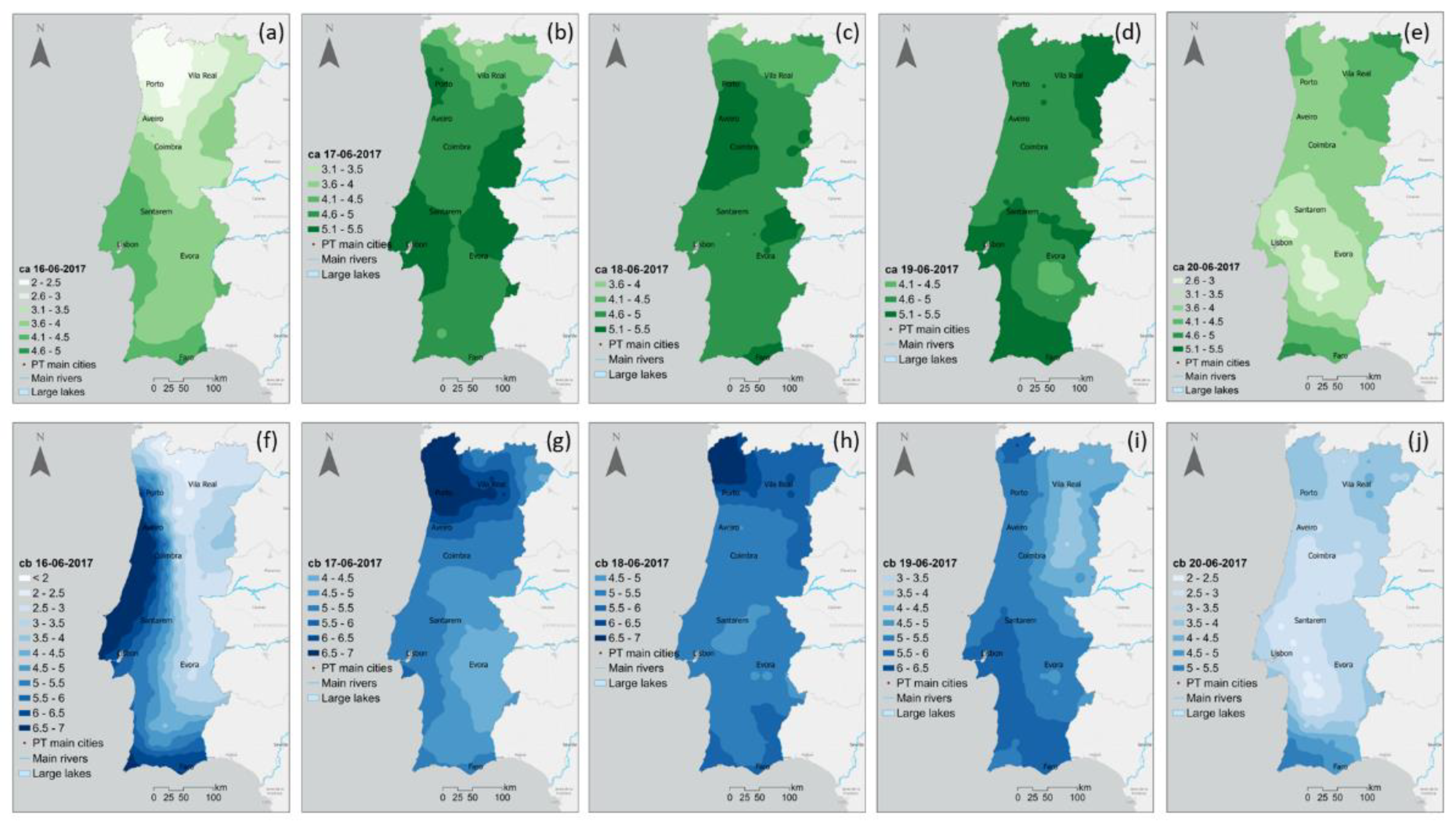
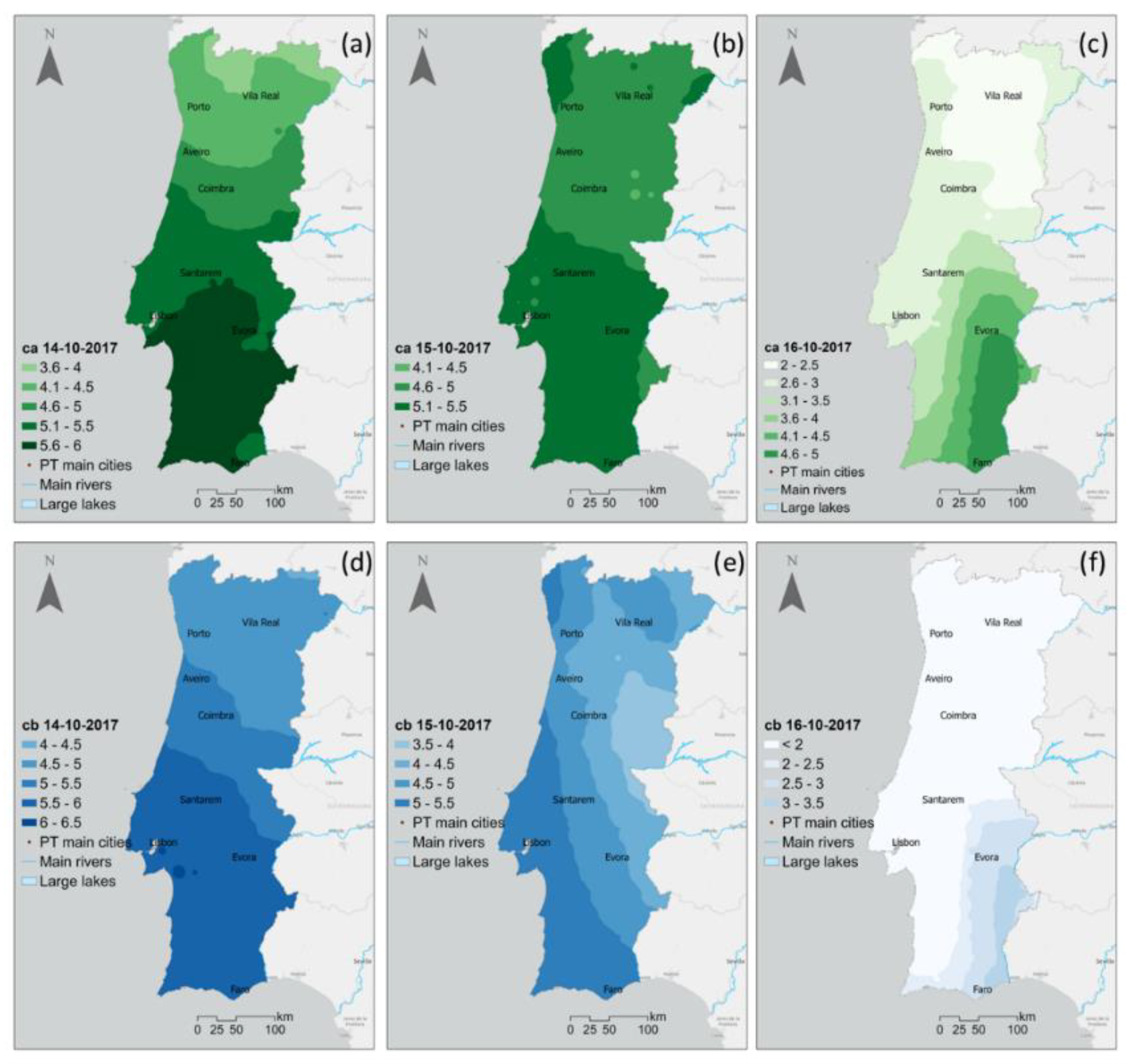
3.2.4. BUI and ERC (Flame Front-Related Components)

The comparison between KBDI and BUI revealed similar spatial patterns (Figure 6f–j) with the highest values in the same locations. The ERC index (Figure 6k–o) variation is due to changes in the moisture content of the various fuels present, both live and dead. Since this number represents the potential “heat release” per unit area in the flaming zone, it can guide several important fire activities. The increasing ERC values between 16 and 17 June (Figure 6k,l) in the regions affected by the great fires point out the relevance of this index for fire risk management.

Similarly, to what was observed in June, in October the spatial distribution of KBDI (Figure 7a–c) and BUI (Figure 7d–f) is again similar and consistent with their intrinsic characteristics (longer timescale variation). Unlike the two previous indices, ERC values, which represent the potential “heat release” per unit area in the flaming zone, prove to be able to capture not only the spatial location of October CEWE (Figure 7g–i) but also that of June (Figure 6k–o).

3.2.5. CHI (Vertical Atmospheric Conditions)

The CHI (Figure 8a–e) and its components linked to instability, namely ca (Figure A7a–e), and cb associated with the dryness in the lower troposphere (Figure A7f–j) showed increasing values between 16 and 18 June. These factors have contributed to a meaningful increase in the danger of the occurrence of wildfires throughout the country, especially on the afternoon of 17 June 2017.

The CHI index also presented high to very high danger values, between 8 and 12.5, on 14 and 15 October, decreasing on 16 October (Figure 9a–c). The component of CHI linked to instability, ca (Figure A8a–c) showed an increase in severity in the central and northern regions, and a decrease in the southern regions, between 14 and 16 October 2017.

The CHI component, linked to moisture in the lowest layer of the troposphere, cb, (Figure A8d–f) showed higher values in the south; and, lower in the north, with an almost zonal stratification, on 14 October (Figure A8d). On 15 October, the highest values of cb were observed on the coast, decreasing inland with a more longitudinal stratification (Figure A8e). On 16 October results show an overall decrease in all components (Figure A8c,f) in clear accordance with the observed meteorological conditions.

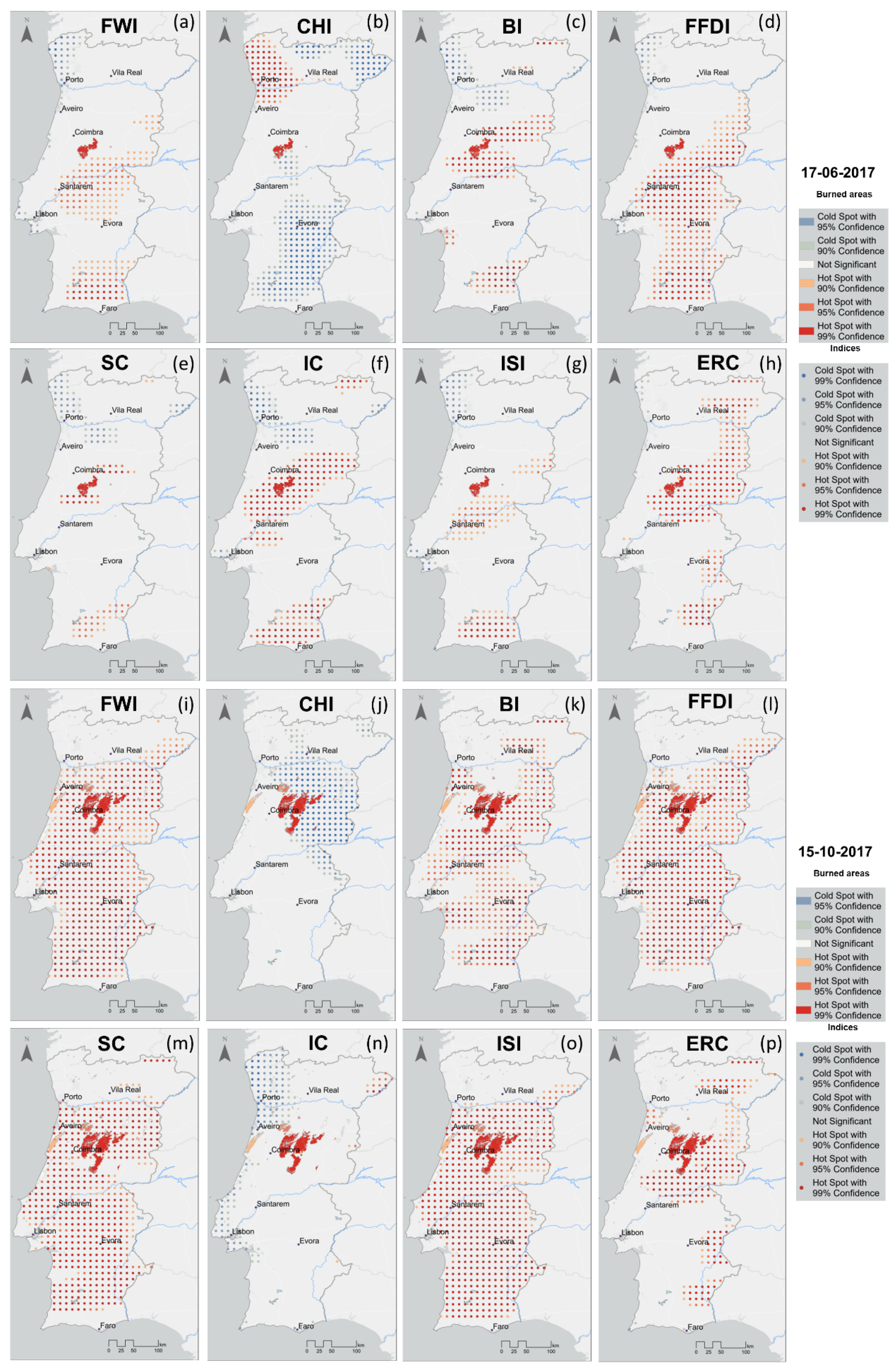
3.3. Hotspot Analysis

The hotspot analysis identifies the clustering of spatial phenomena. It allows the establishment of statistically significant linkages between spatial clusters of high or low values, named hot or cold hotspots between the indices and the burned areas. Overall, this analysis defines statistically significant areas of high or low occurrences (with high or low z-scores). Therefore, the superpositions depicted between the indices and the burned areas above the 90% confidence level (hot hotspots) are highly relevant.

This association is highly pertinent to better understand the relevance of the information that the spatial patterns of each index analyzed in the previous Section 2.2 can provide. It allows us to establish a statistically significant connection between those results in the location of the area most prone to the occurrence of CEWEs. In this case, for succinct purposes, this analysis was undertaken only for the days of the two major 2017 CEWEs. Let us remind you that the hotspot analysis can be performed point-by-point (in this case for each index), as well as for polygons (in this study, for the burned areas). These patterns are depicted in Figure A9 within a statistically meaningful scale color. This color scale ranges from dark red which represents a hot spot with a 99% confidence (followed by a 95% and 90% confidence hot spot). The not-significant hotspots though represented in white in the legend are cleared out from all maps, aiming at highlighting the major statistically significant patterns. This scale ends with a dark blue representing a cold spot with 99% confidence (also followed by a 95% and 90% confidence cold spot).

The hotspot analysis of the burned areas for 17 June and 15 October 2017, (hot hotspots) as well as for all indices FWI, CHI, BI, and FFDI and SC, IC, ISI, and ERC (KDBI and BUI not shown) revealed larger hot hotspot areas for 15 October in comparison with the event in June (Figure A9). The highest z-scores areas are superimposed on the hot hotspots of the burned areas for 15 October for all indices with two exceptions: for CHI for which lower z-scores (cold hotspots) were depicted (Figure A9i)); and for IC with no superimposition, i.e., no statistically significant hotspots were found in the burned areas (Figure A9m). Regarding 17 June, the superimposition of hotspots only occurs for BI, SC, and IC (Figure A9c,e,f). For FWI and FFDI, the highest z-scores are in the vicinity of the burned areas (Figure A9a,d). As for the event in October, for CHI, lower z-scores (cold hotspots) are depicted near the burned areas (Figure A9b). Overall, these results reveal statistically significant spatial connections (above 90% confidence) between most of the indices and the burned areas on 17 June and 15 October 2017. Furthermore, it is worth mentioning that apart from CHI for both events these statistically significant hot hotspots were in the regions for which results in Section 2.3 showed that most of the indices reached their maximum values.

4. Discussion

The ability to supply adequate spatial and temporal forecasts of the potential danger of forest fire ignition and spread is vital. In Portugal, the most applied index is the FWI, which uses surface weather variables. CHI is now also operationally used by IPMA, and in this case, provides further information since it is attained from variables at different pressure levels. This fact helps explain why the hotspot analysis depicted opposite signal z-scores (Figure A9) underlying the different characteristics of these indices. However, since current forecasting is limited and mainly based on a few meteorological variables, the use of other indices proves to be useful.

The year 2017 presented other extreme weather conditions in June [62,63,64], such as a severe heat wave and remarkably high atmospheric instability conditions [45,65,66]. The moisture content of fine fuels measured near the Lousã station was 7% [62] which is consistent with extreme fire danger. These conditions impacted the FWI and CHI indices. This is the case of CHI; even when the meteorological variables, fuel, and orography are steady, atmospheric instability along with a dry environment aloft can promote the spread of a wildfire. The generation of convective heat columns within and around the smoke plume promotes strong air currents which in turn can ignite new fires, spotting, and therefore new fronts [37,45,67,68]. This was the case of the Pedrógão Grande wildfire of June, and the results attained are in clear accordance with the findings of Pinto et al. [45] (Figure 9b and Figure A8b,e) regarding the relevance of the atmospheric instability in this CEWE. This instability promoted conditions prone to the development of a convective thunderstorm system in the southeastern region of Pedrógão Grande that produced a large number of lightning strikes [45].

In the southernmost regions of Portugal, despite the remarkably high FWI values, CEWE did not take place. This can be due to the terrain characteristics as well as vegetation types and ignitions. After 17 June (the Pedrógão Grande wildfire), several other fires occurred in Portugal, mainly in the center of the country, but the most severe event took place on 15 October 2017 (Figure 1b) [65,66].

Outcomes show that the average values of the FWI in mainland Portugal also gradually increased from 14 to 15 October (Figure 5a–c) having reached their highest value from June to 15 October. Overall, these fires presented serious control problems with torching out, crowning, and spotting. In this case, control efforts at the fire head were ineffective due to the adverse conditions of the terrain and vegetation type.

In this study, the results attained for KBDI are in clear accordance with the climatological conditions, with lower values for June (Figure 6a–e) and higher for October (Figure 7a–c), thus translating the drought conditions. The analysis of the daily values of KBDI is consistent with the nature of this index since it builds slowly through time, hence no major variations were depicted for both CEWEs (Figure 6a–e and Figure 7a–c). Due to this fact, the hotspot analysis did not include this index or BUI. The autumn period (from September to November) normally presents a considerable increase in precipitation, which did not take place in 2017. September and October were extremely dry (record breaking-drought in October), and this month was classified as extremely hot, especially the first fortnight. In addition to these long-term factors, the influence of hurricane Ophelia induced a very strong southerly wind that transported hot and dry air from North Africa over most of the territory, thus contributing to the increase of wildfire danger. These conditions led to a record number of wildfires and the largest burnt area in a single day in Portugal on 15 October 2017.

BI provides an estimate of the potential difficulty in containing a fire since it relates to the length of the flame at the head of the fire. The BI also reflects the changes in fine fuel moisture content and wind speed, thus being highly variable day-to-day. Therefore, is more appropriate for a short-term forecast of fire danger, while KBDI is more suitable for a long-term assessment. BI is also a function of the ERC and SC (Figure A2), which is proportional to the spread rate. It is worth emphasizing that FWI and BI are analogous fire danger indices, in which FWI is attained from BUI and ISI, whilst BI is by ERC and SC. Likewise, while BUI and ERC are linked to the moisture content in the largest moisture reservoirs, ISI and SC are associated with the effects of fine fuel moisture content and wind speed. These latter factors impact flaming combustion. Owing to these characteristics, BUI, KBDI, and even ERC have long drying time lags, thus changing slower in comparison with ISI, IC, and SC which changes daily. Results for ISI, IC, and SC are, thus, in clear accordance with their intrinsic characteristics. They show increasingly higher values between the previous day and the day of the big events (Figure A2, Figure A5 and Figure A6) with quite similar spatial patterns for 15 October (Figure A6b,h). These outcomes are also depicted in the hotspot analysis with high hot (high z-score values) hotspot areas superimposed with the burned areas, mainly in October (Figure A9). This result translates into an intense spatial clustering between the indices and the burned areas.

The maximum daily average values of BI, in June for the reference period fluctuated between 29.9 and 38.5, while in 2017 they fluctuated between 23 and 50.8. The maximum BI value (58.125) was observed in 2019 (not shown). These are relatively low values for the BI in the USA, which seems to indicate that the future use of this index in Portugal will require a different scale or interpretation. This fact might also be due to the fuel model, a component for attaining BI that could be adjusted for Portugal. On 17 June, the highest BI value was below 40 (first level on the scale), which would indicate fires that can be attacked at the head or flanks by firefighters using hand tools. The hand line should hold the fire. However, this was not the case in the events that took place in the complex of fires of Pedrógão Grande and Góis. On 15 October 2017, the maximum BI value was 54.104 (Figure 5e) the second-highest value observed within the control period. It should be noted that this value is within the second class of the danger scale and was also higher in comparison with the CEWE of June. For the first fortnight of October, the BI index values were always well above the average (control period and for Portugal) for this month. Overall, it is worth emphasizing that the spatial distribution of BI is quite revealing regarding the location of the complexes of wildfires on 15 October (Figure 5e).

The conclusions for BI point out a new scale or interpretation since for 2017, for both CEWEs, the values observed remain below 40 (first danger class) for June (Figure 4f–j) and only for 15 October go above 40 in the surroundings of the areas affected by the major fire occurrences (Figure 5e). Therefore, when properly adjusted, it can be a useful tool for wildfire forecasting and fire attack planning since it presents the amount of effort needed to contain a fire for a specified fuel type. Jolly et al. [69] presented a severe fire danger index attained from ERC and BI percentiles, along with a previous normalization of the data. This technique might be useful in future work, thus helping to adjust BI and other indices to Portugal, since the conversion of absolute values into percentiles considers the local climatology and therefore simplifies comparisons between regions.

Lastly, the FFDI provides information related to the chances of a fire starting, its rate of spread, its intensity, and the difficulty of suppression. This is done by several combinations of air temperature, relative humidity, and wind speed along with short and long-term drought conditions. This fact helps explain the similar spatial patterns between the FFDI and the FWI (Figure 4 and Figure 5) mainly for the October CEWE (Figure 5a–c). These results are in clear accordance with the ones referenced in the Technical Report of Dowdy et al. [40], which compared the performance of these two indices. Moreover, the FFDI values for October are higher than the ones attained for the great wildfires in June, and the area within the very high danger class is also wider. The hotspot analysis also allowed us to assess a vast high-level z-score region, higher for 15 October fully encompassing the burned areas, thus associated with statistically intense clustering areas (Figure A9h,k). In general, this index also reflects the conditions prone to the occurrence of wildfires.

Overall, the definition of adequate thresholds for the several danger indices for mainland Portugal and the combination of different metrics will provide further information that can be used to support decision-making and help create a new Fire Behavior Prediction Methodology that is more complete than the one that is currently implemented. This methodology should also be able to further enhance the ability to track and predict unique CEWEs since the shortcomings of some indices are compensated by the information retrieved by others, as shown in this study.

5. Conclusions

This study allowed us to conclude that the use of a multi-indices approach to forecasting CEWEs can be advantageous. The main outcomes of the first part of this study are thus summarized herein.

• The maximum and mean monthly values for most of the indices were well above the average in 2017 in comparison with the control period, mainly in June and October. The mean monthly values for June/October of 2017 were statistically significant above the average (TST at a 5% S.L.) except for FFDI/CHI and FFDI, respectively.
• In June for CHI and BI, and in October for BI, statistically significant (MWW test at a 5% S.L.) high positive anomalies were observed in the vicinity of the major CEWEs.
• In September for BI, statistically significant anomalies (MWW test at a 5% S.L.) are already depicted, though with lower values in comparison with October. These results point out the long-term sensitivity of BI regarding CEWEs, even though its limitations are due to the actual scale.

Overall, the results showed the ability of the indices to capture the persistent high-danger conditions prone to the occurrence of wildfires during June and October 2017. This analysis also allowed us to perceive the magnitude of the maximum threshold for each index to assess its ability to predict the wildfire danger in Portugal, thus answering the first main goal of this study.

To answer the other main goals of this study, the second part of this assessment allowed us to conclude that:

All indices were able to capture the increasing variation towards higher danger values from 16 to 17 June and 14 to 15 October 2017.

• All indices presented higher danger values for October in comparison with June, except for CHI. In this case, the highest values were observed in June, thus portraying the contribution of atmospheric instability to the occurrence of this CEWE. Therefore, CHI helps understand the nature of the occurrences, besides the danger level, namely regarding the role of atmospheric instability in these events.
• The daily spatial distributions of FFDI and FWI, as well as KBDI and BUI, are quite similar. These indices can depict the dangerous conditions mainly for 17 June and 15 October. Since the information provided by them can be considered redundant, only one of the two pairs should be used to access the dangerous conditions.
• The spatial distributions of BI, SC, and ERC have had the best performance in capturing the locations for the occurrence of the two CEWEs with statistically significant hot hotspot superimposition areas.
• The ERC patterns revealed the amount of energy released in the locations of the two CEWEs.
• The higher IC values for October clearly show the areas affected by the 15 October wildfires with high values (30–59%) pointing out a high effort to suppress them.
• The spatial patterns of SC and its counterpart ISI, indicate high values associated with high velocities in the spread of these fires for the same target areas.
• The hotspot analysis allowed us to identify the type of clustering between the indices and the burned areas, thus defining statistically significant areas of high and low values.
• High-intensity clustering was depicted in the vicinity of the burned areas mainly for 15 October thus statistically linking the spatial distributions of most of the indices with them.
• For most of the indices, the locations of the statistically significant hot hotspots were depicted in regions in which the indices reached their maximum values. These results demonstrate the relevance of using several indices in helping to understand nature as well as identifying the locations of areas prone to the occurrence of CEWEs. These outcomes can serve as a case study to establish in the future a model to predict the dangerous conditions predisposed to the occurrence of wildfires in Portugal.

Overall, the implementation of a multi-index methodology might be a highly relevant tool for Portugal, whose complex orography and land cover, along with the projected increase in temperatures and intensification in duration and frequency of drought conditions [70,71] will lead to an increase in conditions prone to the occurrence of CEWE. Since this study’s main goals were to provide the first insight, future work will be devoted to assessing the multivariate models that best explain/predict CEWEs. A new forecast methodology can help ensure the development of appropriate spatial preparedness plans, proactive responses by civil protection regarding firefighter management, and suppression efforts, and alert communities to minimize the detrimental impacts of wildfires in Portugal. Lastly, the forecast of the spatial distribution of these events can also be a key factor for a better land management policy, as well as the planning of the country’s forest cover (more fire-resilient species), which should consider prescribed burning techniques (small-scale operations) in locations considered critical [72,73] to reduce the existing build-up load and, thus, the intensity of future fires.

References

1. Pausas, J.G.; Vallejo, V.R. The role of fire in European Mediterranean ecosystems. In Remote Sensing of Large Wildfires; Chuvieco, E., Ed.; Springer: Berlin, Germany, 1999; pp. 3–16. [Google Scholar]
2. Keeley, J.E.; Bond, W.J.; Bradstock, R.A.; Pausas, J.G.; Rundel, P.W. Fire in Mediterranean Ecosystems: Ecology, Evolution and Management; Cambridge University Press: New York, NY, USA, 2011. [Google Scholar]
3. Ager, A.A.; Preisler, H.K.; Arca, B.; Spano, D.; Salis, M. Wildfire danger estimation in the Mediterranean area. Environmetrics 2014, 25, 384–396. [Google Scholar] [CrossRef]
4. Tedim, F.; Xanthopoulos, G.; Leone, V. Forest fires in Europe: Facts and challenges. In Wildfire Hazards, Dangers and Disasters; Paton, D., Ed.; Elsevier: Amsterdam, The Netherlands, 2015; pp. 77–99. [Google Scholar]
5. Fernandes, P.M.; Barros, A.M.G.; Pinto, A.; Santos, J.A. Characteristics and controls of extremely large wildfires in the western Mediterranean Basin. J. Geophys. Res. Biogeo. 2016, 121, 2141–2157. [Google Scholar] [CrossRef]
6. Moreira, F.; Ascoli, D.; Safford, H.; Adams, M.A.; Moreno, J.M.; Pereira, J.M.; Catry, F.X.; Armesto, J.; Bond, W.; González, M.E.; et al. Wildfire management in Mediterranean type regions: Paradigm change needed. Environ. Res. Lett. 2020, 15, 011001. [Google Scholar] [CrossRef]
7. Werth, J.; Werth, P. Haines Index climatology for the western United States. Fire Manag. Notes 1998, 58, 8–17. [Google Scholar]
8. Littell, J.S.; McKenzie, D.; Peterson, D.L.; Westerling, A.L. Climate and wildfire area burned in western U.S. ecoprovinces, 1916–2003. Ecol. Appl. 2009, 19, 1003–1021. [Google Scholar] [CrossRef] [PubMed]
9. Addington, R.N.; Hudson, S.J.; Hiers, J.K.; Hurteau, M.D.; Hutcherson, T.F.; Matusick, G.; Parker, J.M. Relationships among wildfire, prescribed fire, and drought in a fire-prone landscape in the south-eastern United States. Int. J. Wildland Fires 2015, 24, 778–783. [Google Scholar] [CrossRef]
10. Williams, R.J.; Gill, A.M.; Moore, P.H.R. Seasonal Changes in Fire Behaviour in a Tropical Savanna in Northern Australia. Int. Int. J. Wildland Fires 2001, 8, 227–239. [Google Scholar] [CrossRef]
11. Andrade, C.; Contente, J. Köppen’s climate classification projections for the Iberian Peninsula. Clim. Res. 2020, 81, 71–89. [Google Scholar] [CrossRef]
12. Köppen, W.; Geiger, R. Handbuch der Klimatologie; Gebrüder Bornträger: Berlin, Germany, 1930; Volume 6. [Google Scholar]
13. Nunes, A.N. Regional variability and driving forces behind forest fires in Portugal an overview of the last three decades (1980–2009). Appl. Geogr. 2012, 34, 576–586. [Google Scholar] [CrossRef]
14. Fernandes, P.M.; Loureiro, C.; Magalhães, M.; Ferreira, P.; Fernandes, M. Fuel age, weather and burn probability in Portugal. Int. J. Wildland Fire 2012, 21, 380–384. [Google Scholar] [CrossRef]
15. Fernandes, P.M. Variation in the Canadian Fire Weather Index Thresholds for Increasingly Larger Fires in Portugal. Forests 2019, 10, 838. [Google Scholar] [CrossRef] [Green Version]
16. Meneses, B.M. Vegetation Recovery Patterns in Burned Areas Assessed with Landsat 8 OLI Imagery and Environmental Biophysical Data. Fire 2021, 4, 76. [Google Scholar] [CrossRef]
17. Alcasena, F.; Ager, A.; Le Page, Y.; Bessa, P.; Loureiro, C.; Oliveira, T. Assessing wildfire exposure to communities and protected areas in Portugal. Fire 2021, 4, 82. [Google Scholar] [CrossRef]
18. Ribeiro, L.M.; Rodrigues, A.; Lucas, D.; Viegas, D.X. The Impact on Structures of the Pedrógão Grande Fire Complex in June 2017 (Portugal). Fire 2020, 3, 57. [Google Scholar] [CrossRef]
19. Viegas, D.X.; Viegas, M.T. A relationship between rainfall and burned area for Portugal. Int. J. Wildland Fires 1994, 4, 11–16. [Google Scholar] [CrossRef]
20. Potter, B.E. Atmospheric properties associated with large wildfires. Int. J. Wildland Fires 1996, 6, 71–76. [Google Scholar] [CrossRef]
21. Pausas, J.G.; Paula, S. Fuel shapes the fire—Climate relationship: Evidence from Mediterranean ecosystems. Global Ecol. Biogeogr. 2012, 21, 1074–1082. [Google Scholar] [CrossRef]
22. Di Giuseppe, F.; Pappenberger, F.; Wetterhall, F.; Krzeminski, B.; Camia, A.; Libertá, G.; San Miguel, J. The Potential Predictability of Fire Danger Provided by Numerical Weather Prediction. J. Appl. Meteorol. Climatol. 2016, 55, 2469–2491. [Google Scholar] [CrossRef]
23. Vitolo, C.; Di Giuseppe, F.; Krzeminski, B.; San-Miguel-Ayanz, J. A 1980–2018 global fire danger re-analysis dataset for the Canadian Fire Weather Indices. Sci. Data 2019, 6, 190032. [Google Scholar] [CrossRef]
24. Jiménez-Ruano, A.; Mimbrero, M.R.; Jolly, W.M.; de la Riva Fernández, J. The role of short-term weather conditions in temporal dynamics of fire regime features in mainland Spain. J. Environ. Manag. 2019, 241, 575–586. [Google Scholar] [CrossRef]
25. Di Giuseppe, F.; Vitolo, C.; Krzeminski, B.; Barnard, C.; Maciel, P.; San-Miguel, J. Fire Weather Index: The skill provided by the European Centre for Medium-Range Weather Forecasts ensemble prediction system. Nat. Hazards Earth Syst. Sci. 2020, 20, 2365–2378. [Google Scholar] [CrossRef]
26. Haines, D.A.; Main, W.A.; Simard, A.J. Operational validation of the NFDRS in the Northeast. In Proceedings of the Eight Conference on Fire and Forest Meteorology, Detroit, MI, USA, 29 April–2 May 1985; pp. 169–177. [Google Scholar]
27. Van Wagner, C.E. Development and Structure of the Canadian Forest Fire Weather Index System; Forestry Technical Report 35; Canadian Forest Service: Ottawa, ON, Canada, 1987; p. 35. [Google Scholar]
28. Stocks, B.J.; Lawson, B.D.; Alexander, M.E.; Van Wagner, C.E.; McAlpine, R.S.; Lynham, T.J.; Dube, D.E. The Canadian Forest Fire Danger Rating System: An overview. For. Chron. 1989, 65, 450–457. [Google Scholar] [CrossRef]
29. Potter, B.E.; Goodrick, S. Performance of the Haines Index during August 2000 for Montana. In Proceedings of the 4th Symposium on Fire and Forest Meteorology, Reno, NV, USA, 13–15 November 2001; American Meteorological Society: Boston, MA, USA, 2003; pp. 233–236. [Google Scholar]
30. Potter, B.E.; Winkler, J.A.; Dwight, F.W.; Ryan, P.S.; Xindi, B. Computing the low-elevation variant of the Haines Index for fire weather forecasts. Weather. Forecast. 2008, 23, 159–167. [Google Scholar] [CrossRef]
31. Van Wagner, C.E.; Pickett, T.L. Equations and FORTRAN Program for the Canadian Forest Fire Weather Index System; Forestry Technical Report 33; Canadian Forestry Service, Petawawa National Forestry Institute: Chalk River, ON, Canada, 1985; p. 18. [Google Scholar]
32. Viegas, D.X.; Reis, R.M.; Cruz, M.G. Calibração do Sistema Canadiano de Perigo de Incêndio para Aplicação em Portugal. Silva Lusit. 2004, 12, 77–93. [Google Scholar]
33. Carvalho, A.; Flannigan, M.D.; Logan, K.; Miranda, A.I.; Borrego, C. Fire activity in Portugal and its relationship to weather and the Canadian Fire Weather Index System. Int. J. Wildland Fires 2008, 17, 328–338. [Google Scholar] [CrossRef]
34. DaCamara, C.C.; Calado, T.J.; Ermida, S.L.; Trigo, I.F.; Amraoui, M.; Turkman, K.F. Calibration of the Fire Weather Index over Mediterranean Europe based on fire activity retrieved from MSG satellite imagery. Int. J. Wildland Fire 2014, 23, 945–958. [Google Scholar] [CrossRef]
35. Vitolo, C.; Di Giuseppe, F.; Barnard, C.; Coughlan, R.; San-Miguel-Ayanz, J.; Libertá, G.; Krzeminski, B. ERA5-based global meteorological wildfire danger maps. Sci. Data 2020, 7, 216. [Google Scholar] [CrossRef]
36. IPMA. Available online: htttps://www.ipma.pt/pt/media/noticias/newa.detail.jsp?f=/pt/media/noticias/arquivo/2017/rel-clima-outubro-2017.html (accessed on 3 February 2022).
37. EFFIS. Available online: https://effis.jrc.ec.europa.eu/ (accessed on 1 February 2022).
38. Burgan, R.E. 1988 Revisions to the 1978 National Fire-Danger Rating System; Res. Pap. SE-273; U.S. Department of Agriculture; Forest Service, Southeastern Forest Experiment Station: Asheville, NC, USA, 1988; p. 39. [Google Scholar]
39. National Fire Danger Rating System (NFDRS). Van Nostrand’s Scientific Encyclopedia; John Wiley & Sons, Inc.: Hoboken, NJ, USA, 2006. [Google Scholar] [CrossRef]
40. Dowdy, A.J.; Mills, G.A.; Finkele, K.; de Groot, W. Australian Fire Weather as Represented by the McArthur Forest Fire Danger Index and the Canadian Forest Fire Weather Index; CAWCR Technical Report No. 10; Australian Government Bureau of Meteorology: Canberra, Australia. Available online: https://www.google.com/url?sa=t&rct=j&q=&esrc=s&source=web&cd=&ved=2ahUKEwi-3-uaoPn8AhXJUaQEHWD2BdIQFnoECAoQAQ&url=https%3A%2F%2Fwww.cawcr.gov.au%2Ftechnical-reports%2FCTR_010.pdf&usg=AOvVaw1wJCf6EXqchLXtMc6fHcFx (accessed on 13 January 2022).
41. Noble, I.R.; Bary, G.A.V.; Gill, A.M. McArthur’s fire-danger meters expressed as equations. Aust. J. Ecol. 1980, 5, 201–203. [Google Scholar] [CrossRef]
42. Keetch, J.J.; Byram, G.M. A Drought Index for Forest Fire Control; Research Paper SE-38; USDA Forest Service: Asheville, NC, USA, 1968. [Google Scholar]
43. ICNF. Available online: https://fogos.icnf.pt/sgif2010/ (accessed on 31 November 2021).
44. IPMA. Available online: https://www.ipma.pt/pt/riscoincendio/fwi/ (accessed on 1 February 2022).
45. Pinto, P.; Silva, Á.P.; Viegas, D.X.; Almeida, M.; Raposo, J.; Ribeiro, L.M. Influence of Convectively Driven Flows in the Course of a Large Fire in Portugal: The Case of Pedrógão Grande. Atmosphere 2022, 13, 414. [Google Scholar] [CrossRef]
46. Haines, D.A. A lower atmospheric severity index for wildland fire. Natl. Weather. Dig. 1988, 13, 23–27. [Google Scholar]
47. Lawson, B.D.; Armitage, O.B. Weather Guide for the Canadian Forest Fire Danger Rating System; Natural Resources Canada, Canadian Forest Service, Northern Forestry Centre: Edmonton, AB, Canada, 2008; p. 73. [Google Scholar]
48. Palheiro, P.; Fernandes, P.; Cruz, M. A fire behaviour-based fire danger classification for maritime pine stands: Comparison of two approaches. For. Ecol. Manag. 2006, 234 (Suppl. S1), S54. [Google Scholar] [CrossRef]
49. Choi, G.; Kim, J.; Won, M.S. Spatial patterns and temporal variability of the Haines Index related to the wildland fire growth potential over the Korean Peninsula. J. Korean Geogr. Soc. 2006, 41, 168–187. [Google Scholar]
50. Bugalho, L. Temporal variability of the Haines index and its relationship with forest fire in Portugal. In Advances in Forest Fire Research; Chapter 1—Fire Danger Management; Publisher’s Name: Coimbra, Portugal, 2018; pp. 127–137. [Google Scholar] [CrossRef]
51. Luke, R.H.; McArthur, A.G. Bushfires in Australia; Australian Government Publishing Service: Canberra, Australia, 1986; p. 91. [Google Scholar]
52. Wain, A.; Kepert, D. A Comprehensive, Nationally Consistent Climatology of Fire Weather Parameters; Bushfire Cooperative Research Centre: Melbourne, VIC, Australia, 2013. [Google Scholar]
53. EEA. Available online: https://www.eea.europa.eu/ims/forest-fires-in-europe (accessed on 1 February 2022).
54. ICNF. Available online: http://www2.icnf.pt/portal/florestas/dfci/inc/estat-sgif (accessed on 20 August 2019).
55. ICNF—Cartografia da área Ardida. Available online: http://www2.icnf.pt/portal/florestas/dfci/inc/mapas (accessed on 20 August 2019).
56. ECWMF. Available online: https://www.ecmwf.int/en/forecasts/datasets (accessed on 13 January 2022).
57. Copernicus Datasets. Available online: https://cds.climate.copernicus.eu (accessed on 3 January 2022).
58. Wilcoxon, F. Individual comparisons by ranking methods. Biom. Bull. 1945, 1, 80–83. [Google Scholar] [CrossRef]
59. Mann, H.B. Non-parametric tests against trend. Econometrica 1945, 13, 245–259. [Google Scholar] [CrossRef]
60. Walker, B.B.; Schuurman, N.; Hameed, S.M. A GIS-based spatiotemporal analysis of violent trauma hotspots in Vancouver, Canada: Identification, contextualization and intervention. BMJ Open 2014, 4, e003642. [Google Scholar] [CrossRef] [PubMed]
61. Stopka, T.J.; Krawczyk, C.; Gradziel, P.; Geraghty, E.M. Use of spatial epidemiology and hot spot analysis to target women eligible for prenatal women, infants, and children services. Am. J. Public Health 2014, 104 (Suppl. 1), S183–S189. [Google Scholar] [CrossRef]
62. Viegas, D.X.; Almeida, M.F.; Ribeiro, L.M.; Raposo, J.; Viegas, M.T.; Oliveira, O.; Alves, D.; Pinto, C.; Jorge, H.; Rodrigues, A.; et al. O Complexo de Incêndios de Pedrógão Grande e Concelhos Limítrofes, iniciado a 17 de Junho de 2017. Centro de Estudos sobre Incêndios Florestais, CEIF- Universidade de Coimbra. Relatório. 2017, p. 238. Available online: https://www.researchgate.net/publication/339213823_O_complexo_de_incendios_de_Pedrogao_Grande_e_concelhos_limitrofes_iniciado_a_17_de_junho_de_2017/link/5e446d70a6fdccd9659f9efc/download (accessed on 13 January 2022).
63. San-Miguel-Ayanz, J.; Oom, D.; Artes, T.; Viegas, D.X.; Fernandes, P.; Faivre, N.; Freire, S.; Moore, P.; Rego, F.; Castellnou, M. Forest fires in Portugal in 2017. In Science for Disaster Risk Management 2020: Acting Today, Protecting Tomorrow; Casajus Valles, A., Marin Ferrer, M., Poljanšek, K., Clark, I., Eds.; EUR 30183 EN; Publications Office of the European Union: Luxembourg, 2020; ISBN 978-92-76-18182-8. [Google Scholar] [CrossRef]
64. Guerreiro, J.; Fonseca, C.; Salgueiro, A.; Fernandes, P.; Lopez, E.; de Neufville, R.; Mateus, F.; Castellnou, M.; Silva, J.S.; Moura, J.; et al. (Eds.) Análise e Apuramento dos Factos Relativos aos Incêndios que Ocorreram em Pedrógão Grande, Castanheira de Pêra, Ansião, Alvaiázere, Figueiró dos Vinhos, Arganil, Góis, Penela, Pampilhosa da Serra, Oleiros e Sertã entre 17 e 24 de Junho de 2017; Independent Technical Commission, Assembly of the Republic: Lisbon, Portugal, 2017. [Google Scholar]
65. Guerreiro, J.; Fonseca, C.; Salgueiro, A.; Fernandes, P.; Lopez, E.; de Neufville, R.; Mateus, F.; Castellnou, M.; Silva, J.S.; Moura, J.; et al. (Eds.) Relatório: Avaliação dos Incêndios Ocorridos Entre 14 e 16 de Outubro de 2017 em Portugal Continental; Independent Technical Commission, Assembly of the Republic, Lisbon, Portugal, 2018. Available online: https://www.parlamento.pt/Documents/2018/Marco/RelatorioCTI190318N.pdf (accessed on 13 January 2022).
66. Viegas, D.X.; Almeida, M.A.; Ribeiro, L.M.; Raposo, J.; Viegas, M.T.; Oliveira, R.; Alves, D.; Pinto, C.; Rodrigues, A.; Ribeiro, C.; et al. Análise dos Incêndios Florestais Ocorridos a 15 de outubro de 2017; Centro de Estudos sobre Incêndios Florestais: 2019. Available online: https://www.portugal.gov.pt/pt/gc21/comunicacao/documento?i=analise-dos-incendios-florestais-ocorridos-a-15-de-outubro-de-2017 (accessed on 13 January 2022).
67. Tatli, H.; Türkes, M. Climatological evaluation of Haines forest fire weather index over the Mediterranean Basin. Meteorol. Appl. 2014, 21, 545–552. [Google Scholar] [CrossRef]
68. Barberà, M.J.; Niclòs, R.; Estrela, M.J.; Valiente, J.A. Climatology of the stability and humidity terms in the Haines Index to improve the estimate of forest fire risk in the Western Mediterranean Basin (Valencia region, Spain). Int. J. Climatol. 2015, 35, 1212–1223. [Google Scholar] [CrossRef]
69. Jolly, W.M.; Freeborn, P.H.; Page, W.G.; Butler, B.W. Severe Fire Danger Index: A Forecastable Metric to Inform Firefighter and Community Wildfire Risk Management. Fire 2019, 2, 47. [Google Scholar] [CrossRef]
70. Andrade, C.; Contente, J.; Santos, J.A. Climate Change Projections of Dry and Wet Events in Iberia Based on the WASP-Index. Climate 2021, 9, 94. [Google Scholar] [CrossRef]
71. Andrade, C.; Contente, J.; Santos, J.A. Climate Change Projections of Aridity Conditions in the Iberian Peninsula. Water 2021, 13, 2035. [Google Scholar] [CrossRef]
72. Fernandes, P.M.; Davies, G.M.; Ascoli, D.; Fernández, C.; Moreira, F.; Rigolot, E.; Stoof, C.R.; Vega, J.A.; Molina, D. Prescribed burning in southern Europe: Developing fire management in a dynamic landscape. Front. Ecol. Environ. 2013, 11, e4–e14. [Google Scholar] [CrossRef] [Green Version]
73. Fernandes, P.M.; Rossa, C.G.; Madrigal, J.; Rigolot, E.; Ascoli, D.; Hernando, C.; Guiomar, N.; Guijarro, M. Prescribed burning in the European Mediterranean Basin. In Global Application of Prescribed Fire, 1st ed.; CRC Press: Boca Raton, FL, USA, 2022; Chapter 13; pp. 230–248. ISBN 9781032137179. [Google Scholar]
Figure 2. Mainland Portuguese administrative regions (districts) superimposed with the total burned area (a) for June (54,953 ha) and (b) October 2017 (313,794 ha) (Note that only the major wildfires were considered; and, the burned area polygons were attained from ICNF, the Portuguese rural fire database ([43,53,54,55], accessed on 31 November 2021)).
Fire 06 00056 g002
Figure 3. Spatial distribution of the statistically significant (at a 5% significance level) monthly mean anomalies for FWI, CHI, KBDI, BI, and FFDI between 2001–2021 (reference period), respectively by row and 2017 for (a,g,m,s,aa) May, (b,h,n,t,ab) June, (c,i,o,u,ac) July, (d,j,p,v,ad) August, (e,k,q,x,ae) September, and (f,l,r,z,af) October (Note that the MWW test was performed point-by-point at a 5% significance level).
Fire 06 00056 g003
Figure 4. Daily mean values for (a,f,k) 16, (b,g,l) 17, (c,h,m) 18, (d,i,n) 19, and (e,j,o) 20 June 2017, for FWI (upper row), BI (middle row), and FFDI (lower row).
Fire 06 00056 g004
Figure 5. Daily mean values for (a,d,g) 14, (b,e,h) 15, and (c,f,i) 16 October 2017, for FWI (upper row), BI (middle row), and FFDI (lower row).
Fire 06 00056 g005
Figure 6. Daily mean values for (a,f,k) 16, (b,g,l) 17, (c,h,m) 18, (d,i,n) 19, and (e,j,o) 20 June 2017, for KBDI (upper row), BUI (middle row), and ERC (lower row).
Fire 06 00056 g006
Figure 7. Daily mean values for 16 (a,d,g), 14 (b,e,h), and 15 October (c,f,i) 2017, for KBDI (upper row), BUI (middle row), and ERC (lower row).
Fire 06 00056 g007
Figure 8. Daily mean values for (a) 16, (b) 17, (c) 18, (d) 19, and (e) 20 June 2017, for CHI.
Fire 06 00056 g008
Figure 9. Daily mean values for (a) 14, (b) 15, and (c) 16 October 2017, for CHI.
Fire 06 00056 g009