A Multimodal Data Fusion and Deep Learning Framework for Large-Scale Wildfire Surface Fuel Mapping

Abstract

Accurate estimation of fuels is essential for wildland fire simulations as well as decision-making related to land management. Numerous research efforts have leveraged remote sensing and machine learning for classifying land cover and mapping forest vegetation species. In most cases that focused on surface fuel mapping, the spatial scale of interest was smaller than a few hundred square kilometers; thus, many small-scale site-specific models had to be created to cover the landscape at the national scale. The present work aims to develop a large-scale surface fuel identification model using a custom deep learning framework that can ingest multimodal data. Specifically, we use deep learning to extract information from multispectral signatures, high-resolution imagery, and biophysical climate and terrain data in a way that facilitates their end-to-end training on labeled data. A multi-layer neural network is used with spectral and biophysical data, and a convolutional neural network backbone is used to extract the visual features from high-resolution imagery. A Monte Carlo dropout mechanism was also devised to create a stochastic ensemble of models that can capture classification uncertainties while boosting the prediction performance. To train the system as a proof-of-concept, fuel pseudo-labels were created by a random geospatial sampling of existing fuel maps across California. Application results on independent test sets showed promising fuel identification performance with an overall accuracy ranging from 55% to 75%, depending on the level of granularity of the included fuel types. As expected, including the rare—and possibly less consequential—fuel types reduced the accuracy. On the other hand, the addition of high-resolution imagery improved classification performance at all levels.

1. Introduction

Statistics show an unprecedented increase in the size, intensity, and effects of wildfire events relative to historical records [1,2]. In 2018, the deadliest fire in California history, the Camp Fire, resulted in 85 casualties and destroyed nearly 14,000 homes and more than 500 commercial structures [2]. Exacerbated by climate change, extreme wildfires are projected by the United Nations Environment Program to further increase globally on the order of 30% by 2050 and 50% by the end of the century [3]. Wildfires are continuing to grow into a substantial threat to the well-being of communities and infrastructure despite technological and theoretical advancements in fire science. The unprecedented size and complexity of this problem call for multi-disciplinary and data-informed research on wildfire risk management (assessment, mitigation, and response).

Efficient wildfire risk management relies on accurate wildfire spread simulations. Such simulations can substantially improve the effectiveness of pre-event mitigation, as well as evacuation, rescue, and fire suppression efforts [4,5]. A key input to wildfire simulations is robust estimates of fuels that carry wildfires. Fuels are mainly categorized into the three layers of ground (litter, duff, and coarse woody debris), surface (grass, forb, shrubs, large logs), and canopy fuels (trees and snags) [6]. Although surface fuels are the primary drivers of the initiation and spread of forest fires, research in this area has matured slowly with the Anderson 13-category standard fire models [7], which served as the primary input for point-based and spread simulations until the inclusion of the 40 Scott and Burgan standard fire behavior models introduced in 2005 [8]. Surface fuel characterization methods were developed as generalizations, which did not capture the full range of temporal variability and spatial non-conformity that are inherent in surface fuel beds [6]. Therefore, input data into modern fire behavior models bear uncertainties in describing the dynamic processes that are missed in traditional fuel inventories [9]. A review of the state of the art in surface fuel mapping research indicates that most of the past research efforts were focused on site-specific semi-manual expert systems or traditional machine learning methods (e.g., decision trees and random forests) at regional scales. These systems have limited capability in leveraging big data analytics, which can be exploited to learn from spatial and spectral continuities and provide consistency of vegetation and fuels across a given landscape. As a result, such systems are difficult to generalize to large problem domains.

At the national scale, the LANDFIRE program has created comprehensive and consistent geospatial fuel products that incorporate remote sensing with machine learning, expert-driven rulesets, and quality control [10]. Although these products have created a valuable foundation for fire spread simulation efforts based on years of collective experience and domain expertise, large-scale modeling techniques are needed that deliver near-real-time on-demand fuel mapping based on georeferenced fuel data and do not rely on experience-driven expert rulesets and localized vegetation models [11]. Such models could improve the frequency and reduce the latency of fuel data, which are currently at a multi-year level. Furthermore, new techniques could allow for a comprehensive and systematic accuracy assessment using independent validation datasets, which are currently unavailable for LANDFIRE fuel maps.

To build on the success of the LANDFIRE products as a baseline and improve their capabilities, this paper describes a deep-learning-based framework that ingests multimodal—i.e., hyperspectral satellite, high-resolution aerial image, and biophysical climate and terrain—data. This framework relies on a deep network of layers of learnable weights that are trained using large amounts of georeferenced labeled data that guide the formation of the data extraction pipeline.

Background. Most past efforts to map surface fuels for wildfire spread simulations utilize fire behavior fuel models, which are abstract categorizations of fuels that are used as input in fire spread simulations. The most widely adopted model in the United States was developed by Scott and Burgan, which has 40 fuel categories [8]. Most of the past work on fuel identification and mapping focused on classifying the pixels of a georeferenced map into one of the fire behavior fuel model categories. A review of the fuel identification and mapping literature shows a variety of approaches leveraging remote sensing and biophysical data.

Table 1. Summary of surface fuel mapping literature: comparison of training scale and applicability.

Inputs	Region of Interest	Training Set	Target Fuel Model	Reference
Spectral indices, topography, climate	40,000-km2 area in British Columbia, Canada	Sample of 450,000 pixels from the Canadian Fuel Layer	Canadian Forest Fire Behavior System	[12]
Lidar and AVIRIS data	395-km2 area of the 2014 King Fire, California, USA	N/A	Anderson 13 fuel model	[13]
ASTER satellite data	212-km2 area in the Canary Islands, Spain	Sample of pixels from existing fuel map	Scott and Burgan 40 fuel model	[14]
Airborne laser scanning and Indian Satellite data	Two areas of 165 km2 and 487-km2 in Sicily, Italy	5028 field plots	NFFL fuel model	[15]
Lidar data	410 km2 national park in Spain	128 field plots	Prometheus fuel model	[16]
ASTER imagery	64-km2 region in the south of Italy	17 field plots (500 pixels)	Modified Prometheus fuel model	[17]
Lidar data and bands of NAIP imagery	99.5 km2 of northern Sierra Nevada, California	N/A	Scott and Burgan 40 fuel model	[18]
Lidar and Airborne Thematic Mapper data	2.3 km2 of a national park in Spain	360 field plots	Prometheus fuel model	[19]
Lidar and Quickbird data	13-km2 area in eastern Texas, USA	27 polygons (2160 pixels)	Anderson 13 fuel model	[20]
ALS data, Landsat-8 data, and Digital Terrain Model	3678-km2 area in the Canary Islands, Spain	2548 points	NFFL and Canary Islands Fuel Classification model	[21]
Landsat imagery and Digital Elevation Model	410-km2 national park in Spain	Sample from 102 field plots	Modified Prometheus fuel model	[22]
Lidar data and WorldView-2 imagery	15-km2 island in the Canary Islands, Spain	40 field plots	Prometheus fuel model	[23]
Airborne Laser Scanner and Sentinel 2 data	2023-km2 forest in Spain	136 field plots	Prometheus fuel model	[24]
USFS Integrated Resource Inventory data	715-km2 area in Boulder, Colorado	196 field plots	Scott and Burgan 40 fuel model	[25]
ASTER imagery	250-km2 area in Idaho	107 field plots	NFFL fuel model	[26]
Quickbird, Landsat-TM, and EO-1 Hyperion imagery	60-km2 area in Greece	N/A	Own-developed six classes	[27]

N/A: Not using supervised learning. USFS: United States Forest Service. NFFL: Northern Forest Fire Laboratory.Table 1 also includes several research studies that have used lidar data, with or without spectral signatures, as inputs to fuel identification models. Stavros et al. [13] used height information from lidar together with AVIRIS data to build a heuristic fuel map with inconclusive fuel identification performance. Huesca et al. [16] used lidar data to compare Spectral Mixture Analysis, Spectral Angle Mapper, and Multiple Endmember Spectral Mixture Analysis mapping methods for fuel mapping in a national forest in Spain. Mutlu et al. [20] showed that fusing lidar data resulted in fuel identification improvement compared with using Quickbird multispectral imagery alone. Jakubowski et al. [18] estimated the fuel map for a small region in the Sierra Nevada using lidar data and National Agricultural Imagery Program (NAIP) imagery, and a variety of traditional machine learning algorithms, and concluded that although the methods predicted general fuel categories accurately, specific fuel type prediction accuracy was poor. Garcia et al. [19] reported high fuel identification accuracy using lidar and spectral data with Support Vector Machines and decision rules and attributed the cases of confusion to low lidar penetration to understory vegetation. These studies indicate that, while the inclusion of lidar data has shown promise, their limited spatial availability has restricted their applicability to small scales. Therefore, until frequent high-resolution lidar surveys become available at the national scale, this data modality might not be a useful input for large-scale mapping efforts.

summarizes the major studies on surface fuel identification and mapping. We note here that our paper focuses only on surface fuels. Therefore, the term fuel will be used hereafter to refer to surface fuels only.

The studies listed in Table 1 mostly use spectral signatures from satellite or airborne imagers, lidar data, biophysical data, or a combination thereof to identify and map fuels. In most cases, the area of interest is less than a few hundred square kilometers, and the labeled training data comprise only small numbers of points. This means that the resulting fuel identification models are localized and site-specific. The closest work to large-scale fuel identification is that of Pickel et al. [12], wherein the utility of an Artificial Neural Network model for fuel mapping was explored. They used a three-layer neural network to estimate 9 fuel types based on the Canadian Fire Behavior Prediction System for a 200 × 200 km² area in British Columbia, using a vector of 24 spectral, terrain, and climate inputs. For the target fuel labels, their work used a sample of pixels from the Canadian fuel product. The results of the study demonstrated that an overall accuracy of 60–70% could be achieved after regrouping the less-frequent fuel types.

The review of the literature in Table 1 also shows that, while different sources of imagery have been used to extract multispectral information at the points of interest, high-resolution images have not been used yet as an independent input to identify fuels. In the cases where high-resolution aerial or satellite optical images (e.g., NAIP and Quickbird imagery) have been used ([18,23,27]), only RGB pixel values were collected as scalar inputs similar to other spectral or biophysical features. In Mutlu et al. [20]—while bands of 2.5-m resolution Quickbird images were used to create composite images with lidar-generated bands of height bins, variance, and canopy cover—per-pixel classification using decision rules essentially resulted in the treatment of pixels in isolation, rather than within the landscape context. Therefore, an investigation of the application of high-resolution images as distinct inputs for fuel identification is lacking and would be useful.

The literature review also reveals that none of the previous approaches provide a measure of fuel identification uncertainty. Such uncertainty is well-recognized to exist within any identification task and can be a result of a variety of sources, including randomness in the data, models, and sensors, as well as environmental noise. Knowledge of the uncertainty in the identified fuels is important as it provides a means to account for wildfire simulation uncertainties, which can be helpful in risk assessment and uncertainty-aware decision-making [28]. Furthermore, knowledge of the confidence with which fuels are predicted can be a useful tool for model diagnostics and quality control. In other words, increased uncertainty in the identification can point to underlying problems in the data and, thus, to methods that can be used to improve their accuracy. Specifically, the active learning framework in machine learning aims to improve model performance while reducing the costs associated with large-scale data labeling by actively querying ground truth labels for data points with the highest uncertainty. Providing fuel identification uncertainties would enable the use of active learning to improve fuel identification efforts in the future.

Research Significance. To overcome the current limitations in fuel mapping using remote sensing, this paper leverages emerging deep learning technology to examine the feasibility of creating surface fuel maps at a much larger scale than the existing fuel mapping capabilities, while quantifying fuel map uncertainty. To that end, we use a data fusion scheme to integrate spectral and biophysical features with high-resolution imagery and identify surface fuels using a single end-to-end model for the State of California. To train the model, fuel pseudo-labels are generated using a geospatial sampling of the LANDFIRE fuel maps. This information is then coupled with multimodal input data sourced from various data repositories and geospatial data products, including multispectral satellite data (bands of Landsat surface reflectance), spectral indices (e.g., Normalized Difference Vegetation Index (NDVI)), topography and terrain data (from the U.S. Geological Survey (USGS) Digital Elevation Model), and high-resolution aerial imagery from the NAIP. The proposed approach presents the following technical contributions and benefits with respect to the existing literature:

• Creating fuel identification models that are applicable at large spatial scales (e.g., state and national levels) while integrating spectral and biophysical information with high-resolution imagery and providing a measure of model uncertainty;
• Creating a method for anomaly detection in the existing surface fuel mapping systems (specifically the LANDFIRE products) by comparing the predicted fuels with the existing fuel labels and using the discrepancies as a starting point for quality control;
• Providing a means to interpolate fuels for the intermediate years when fuel maps are not available within the LANDFIRE database.

A detailed analysis of the effect of the individual components of the model, the proposed stochastic ensemble approach, and the size of the dataset utilized for model training is presented in the discussions. It should be noted that the use of pseudo-labels sampled from the LANDFIRE products is to demonstrate the proof-of-concept and examine the feasibility of developing large-scale fuel identification models. However, the proposed framework is readily applicable to large collections of field data from national data collection campaigns, such as the Forest Inventory and Analysis (FIA) program of the United States Forest Service, which is not publicly available at this time [29].

2. Materials and Methods

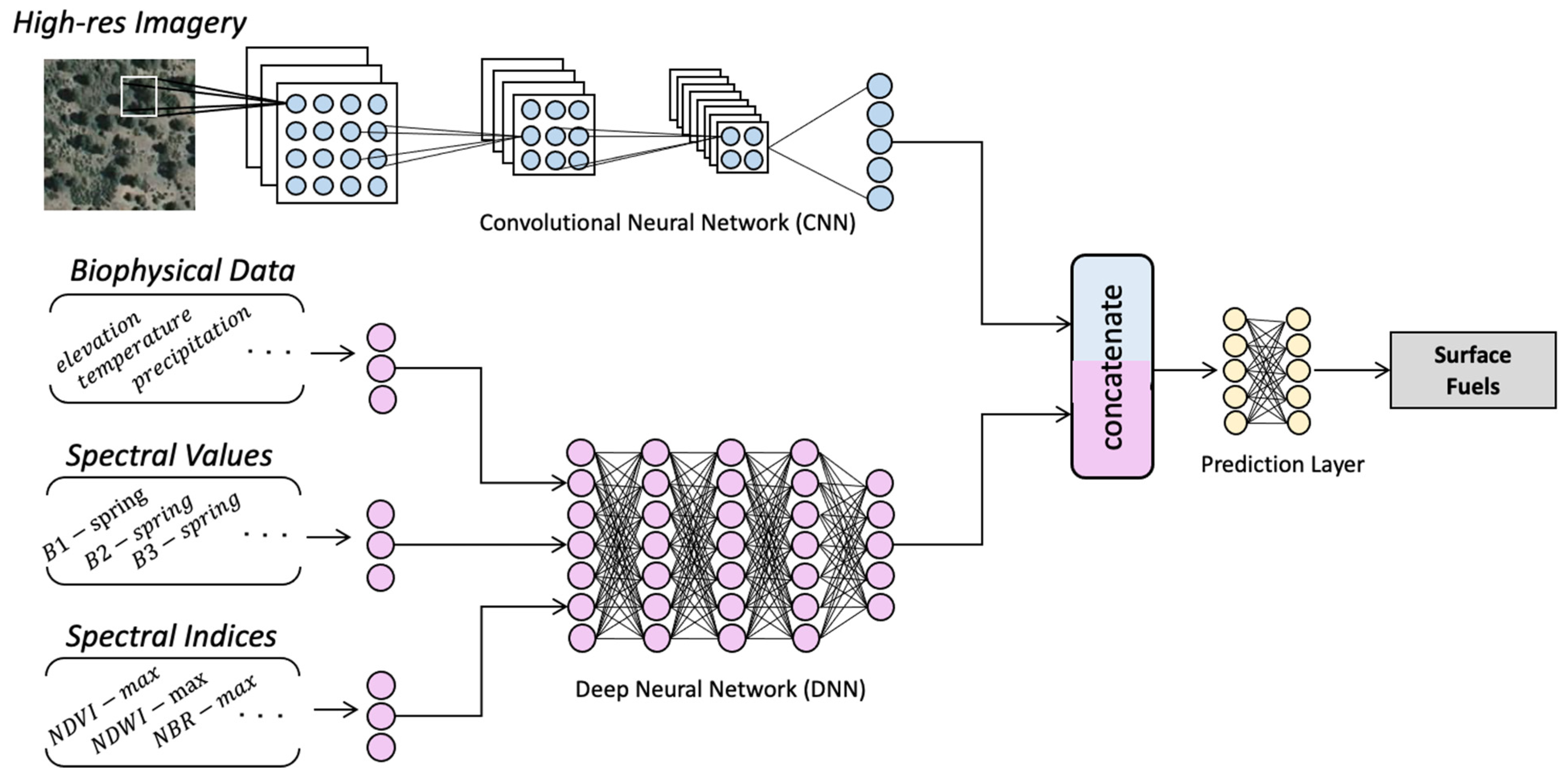
Proposed System. This paper investigates the use of deep learning for large-scale surface fuel mapping. Figure 1 provides a schematic of the proposed identification model where two types of neural networks are used to extract information from different modalities of input data in a way that facilitates their fusion and end-to-end training on labeled data. For tabular data—such as biophysical metadata (e.g., terrain and climate features), seasonal spectral values (e.g., bands of Landsat multispectral imagery), and statistics of spectral indices (e.g., NDVI), a multi-layer artificial neural network (ANN) consisting of multiple fully connected neural layers is used. For image-based contextual data (i.e., high-resolution imagery), a convolutional neural network (CNN) is used, which leverages a deep hierarchy of stacked convolutional filters that constitute layers of increasingly meaningful visual representations. The number, arrangement, and characteristics of these layers can be designed for each specific task. Alternatively, a variety of state-of-the-art CNN architectures exist that can be utilized as backbones and outfitted with custom dense output layers. Examples of these architectures include VGGNet [30], ResNet [31], DenseNet [32], Inception [33], and InceptionResNet [34]. These architectures have been used in several remote sensing applications with different degrees of success [35], and the selection of the optimal architecture is known to be dependent on the characteristics of the specific task at hand. In this work, an array of architectures is trained and compared with each other to maximize fuel identification performance. To speed up and improve the learning process, a learning mode called transfer learning can be used, wherein the extracted features in state-of-the-art CNN architectures that have been pre-trained on generic large-scale computer vision datasets are repurposed and fine-tuned to the existing task. This is built upon the widely known observation that the intermediate visual features extracted in visual recognition tasks are not entirely task-specific, except for the final classification layer [36,37]. Even in cases with a large distance between the source and target tasks, transferring features from networks pre-trained on large datasets is better than random initialization [36]. This has been shown to be applicable to various remote sensing problems involving RGB imagery [38,39,40]. In remote sensing applications involving spatial data other than RGB imagery (e.g., multi/hyper-spectral data, lidar, and radar images), the number and nature of input bands are usually not consistent with such pre-trained networks. However, in the proposed approach, the application of the CNN backbone on high-resolution RGB imagery allows for the use of transfer learning. As a result, the weights of the CNN backbone are initialized from those pre-trained on the generic computer vision ImageNet dataset [41], which are then fine-tuned using the high-resolution fuel imagery herein.

At the conclusion of each neural network branch, the computed features are concatenated before the final prediction layer to fuse the multimodal data. The optimal share of the branches in the data fusion will be determined through training in terms of the weights of the prediction layers. This end-to-end architecture is shown in Figure 1, which is built upon the established notion that different modalities of sensing the same subject usually provide complementary information, enabling deep learning methods to produce more reliable predictions. Details on the network and data fusion design are presented in a later section.

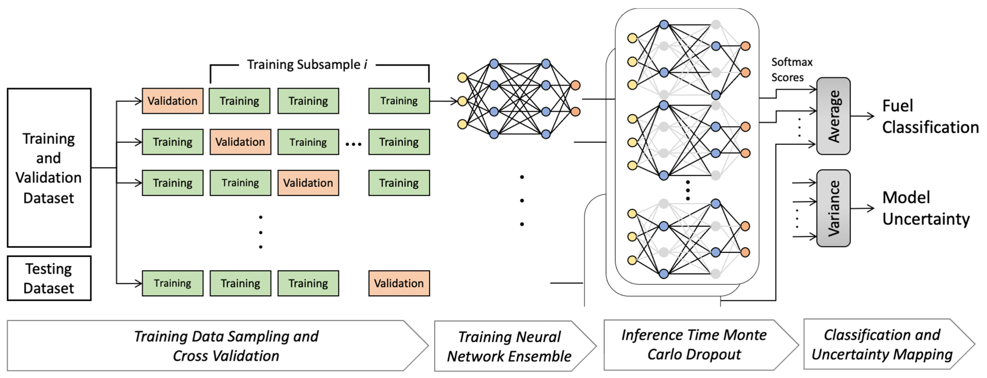
Training the same machine learning model on different sets of observations from the same population has been shown to result in a degree of variance in the resulting models [42]. Furthermore, aside from the CNN backbone that is initialized from pre-trained weights according to transfer learning, all other neural network layers are randomly initialized, resulting in slightly different models, some of which may not provide optimal fuel identification results. To improve the accuracy and robustness of the model in response to variations in observation subsets and training randomness, and to provide a measure of model uncertainty, a stochastic ensemble of models was created, which is depicted in Figure 2.

In the proposed model, the dataset is first randomly split into multiple subsets for training and validation, following the widely used k-fold cross-validation scheme. A separate randomly initialized model is trained on each of the training subsamples to capture the variance from the randomness in the observations. Subsequently, each of these k models is further randomized in inference mode using a process called Monte Carlo dropout [43]. Dropout refers to a regularization technique in neural networks that was originally proposed to combat overfitting by applying a binary mask drawn from a Bernoulli distribution, which has the effect of randomly dropping some of the nodes in the network during training [44]. This, in turn, is known to prevent complex co-adaptation between nodes and can result in improved robustness of trained models [44].

Monte Carlo dropout [43] has been proposed as a mechanism specific to neural networks that aims to quantify machine learning model uncertainties and improve their robustness. In this process, dropout layers embedded before every dense layer in the network are activated at testing time, and the model is applied m times on each observation resulting in m different neural network models where a fraction of the nodes are deactivated at random, hence creating a stochastic ensemble of many slightly perturbed models. Gal and Ghahramani [43] demonstrated that using the mentioned dropout scheme at the testing time provides an approximation of Bayesian inference over the neural network weights that is computationally efficient. This technique has been successfully utilized to derive model uncertainty in visual scene understanding [45], medical imaging [46], robotics, and autonomous driving [47]. However, aside from a few recent applications in road segmentation from synthetic aperture radar [48], ocean hydrographic profiles [49], lunar crater detection [50], and urban image segmentation [51], its applications in remote sensing and especially in wildfires have been limited.

To account for the variations from observation subsets and training randomness by means of the stochastic model ensemble proposed in this work, an overall array of $k \times m$ softmax scores are created for each data point. Lastly, the average of the softmax scores is used to arrive at the final fuel identification, and the variance of the probability scores provides a measure of model uncertainty. Figure 2 depicts this process and its components schematically. In this figure, the arrows at the conclusion of the process denote the softmax scores from each one of the individual models acting on each pixel’s inputs, whose average and variance determine the fuel type classification and its uncertainty, respectively.

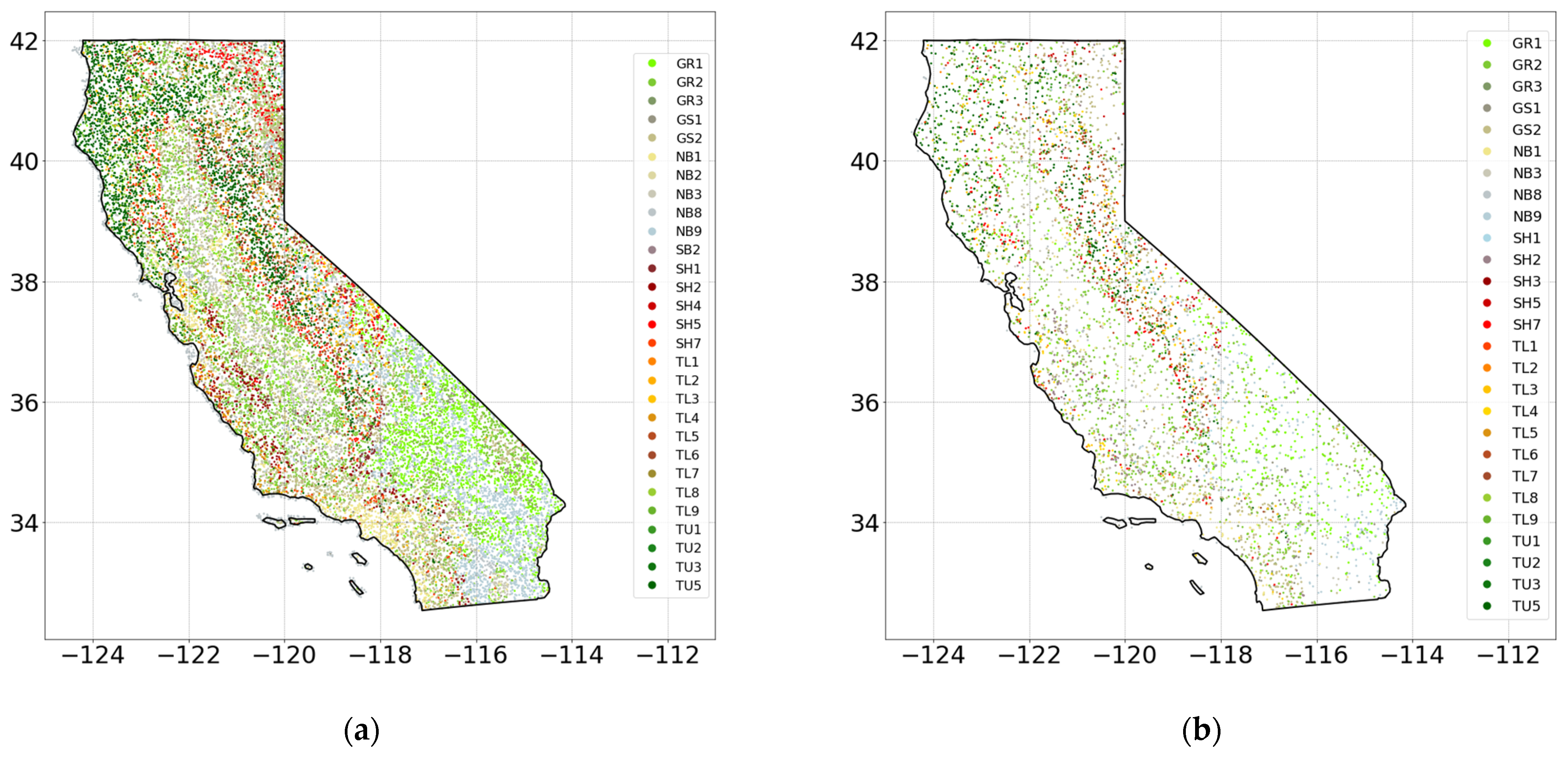
Area of Study. To investigate the feasibility of creating a large-scale fuel identification model using deep learning, the state of California was selected as the area of study for data extraction and model training. To train the system, fuel labels were generated by a random geospatial sampling of the 2016 LANDFIRE Scott and Burgan 40 fuel model. An initial sample of 40,000 points was generated to provide a large training and validation dataset to test the feasibility of training large-scale deep learning models. However, smaller subsets of data were also later created to study the effects of the number of training samples on the performance of the model. This dataset is then divided into training and validation subsets for cross-validation as previously described. Figure 3a depicts the spatial distribution of the collected training samples. To create a means for evaluating the developed models, a random test set was also independently generated. To avoid the proximity and correlation of training and testing samples that could affect the generalizability of the testing results, a minimum distance of 1 mile was enforced between the training and testing samples. This eliminates the possibility of very similar points ending up in both the training and testing sets, which can lead to overly optimistic results. An initial sample of 5000 points was selected for testing (Figure 3b). Fuel type labels in Figure 3 are based on the Scott and Burgan fuel models [8], as presented in

Table 2. Fuel type description based on the Scott and Burgan fuel models adapted from [8].

Fuel Type	Fuel Description
GR1	Grass: Nearly pure grass and/or forb type.	The grass is short, patchy, and possibly heavily grazed. The spread rate is moderate; flame length is low.
GR2		Moderately coarse continuous grass with an average depth of about 1 foot. Spread rate is high; flame length is moderate.
GR3		Very coarse grass, with an average depth of about 2 feet. Spread rate is high; flame length is moderate.
GS1	Grass-Shrub: Mixture of grass and shrub, up to about 50 percent shrub coverage.	Shrubs are about 1 foot high with a low grass load. The spread rate is moderate; flame length is low.
GS2		Shrubs are 1 to 3 feet high, with moderate grass load. The spread rate is high; flame length is moderate.
SH1	Shrub: Shrubs cover at least 50 percent of the site; the grass is sparse to nonexistent.	Low shrub fuel load, fuel bed depth of about 1 foot; some grass may be present. The spread rate is very low; flame length is very low.
SH2		Moderate fuel load (higher than SH1), depth is about 1 foot, no grass fuel present. The spread rate is low; flame length is low.
SH5		Heavy shrub load, depth 4 to 6 feet. The spread rate is very high; flame length is very high.
SH7		Very heavy shrub load, depth 4 to 6 feet. The spread rate is lower than SH5, but the flame length is similar. The spread rate is high; flame length is very high.
TU1	Timber-Understory: Grass or shrubs mixed with litter from the forest canopy.	Fuel bed is low-load grass and/or shrub with litter. The spread rate is low; flame length is low.
TU2		The fuel bed is a moderate litter load with a shrub component. The spread rate is moderate; flame length is low.
TU3		The fuel bed is a moderate litter load with grass and shrub components. The spread rate is high; flame length is moderate.
TU5		The fuel bed is a high-load conifer litter with shrub understory. The spread rate is moderate; flame length is moderate.
TL1	Timber Litter: Dead and down woody fuel (litter) beneath the forest canopy.	Light to moderate load, fuels 1 to 2 inches deep. The spread rate is very low; flame length is very low.
TL2		Low load, compact. The spread rate is very low; flame length is very low.
TL3		Moderate load conifer litter. The spread rate is very low; flame length is low.
TL4		Moderate load, including small-diameter downed logs. The spread rate is low; flame length is low.
TL5		High load conifer litter; light slash or mortality fuel. The spread rate is low; flame length is low.
TL6		Moderate load, less compact. The spread rate is moderate; flame length is low.
TL7		Heavy load, including larger-diameter downed logs. The spread rate is low; flame length is low.
TL8		Moderate load and compactness may include a small amount of herbaceous load. The spread rate is moderate; flame length is low.
TL9		Very high load, fluffy. Spread rate moderate; flame length moderate.
NB1	Non-burnable: Insufficient wildland fuel to carry wildland fire under any condition.	Urban or suburban development; insufficient wildland fuel to carry wildland fire.
NB3		Agricultural field, maintained in non-burnable condition.
NB9		Bare ground.

.

Data Extraction. For each data point in the extracted sample, an array of input features was extracted.

Table 3. Geospatial datasets used for deriving predictors and class variables.

Data Category	Source Dataset	Derived Data
Spectral	Landsat Operational Land Imager (OLI)/Thermal Infrared Sensor (TIRS) seasonal surface reflectance values	Band 2 (blue), band 3 (green), band 4 (red), band 5 (near infrared), band 6, 7 (shortwave infrared 1, 2), band 10, 11 (brightness temperature)
	Landsat annual spectral index statistics (see Table 4 for definitions)	Annual median, minimum, maximum, and range of {NDVI, EVI, SAVI, MSAVI, NDWI, VARI, TCB, TCG, TCW, NBR}
Biophysical	USGS Digital Elevation Model (DEM) with 1/3 arc-second resolution [55]	Elevation (m), computed slope (deg.) and aspect (deg.), multi-scale topographic position index (mTPI)
	PRISM historical climate normal [56]	Mean temperature (°C), mean maximum and minimum temperatures (°C), precipitation (mm), mean dew point temperature (°C), minimum and maximum vapor pressure deficit (hPa), horizontal, sloped, and clear sky solar radiation (MJ m−2 day−1)
Imagery	National Agricultural Imagery Program (NAIP), 1-m resolution [57]	Three-channel (RGB) image centered at the point of interest
Surface Fuels	LANDFIRE 2016 map of standard surface fire behavior fuel models [10] (based on Scott and Burgan 40 fuel models)	Surface fuel types

summarizes the input features used in the modeling, which was informed by the fuel mapping literature reviewed in the background section. Multispectral data are the most widely used data for wildfire fuel modeling, with the Landsat mission being one of the primary sources of open data for these applications [52]. The atmospherically corrected and orthorectified Landsat-8 Operational Land Imager and Thermal Infrared Sensor (OLI/TIRS) surface reflectance data were used at 30-m resolution. A seasonal composite of Landsat OLI/TIRS data was computed for each sample location using the medoid compositing criterion [53]. This criterion minimizes the sum of Euclidean distances in the multispectral space to all other observations over the time period of interest (i.e., seasons). This method selects seasonal representative values while preserving the relationships between the bands and has been shown to produce radiometrically consistent composites [54]. The quality assessment (QA) band codes were utilized to mask pixels contaminated with cloud and cloud shadow.

In addition to the seasonal spectral values, annual statistics of well-established spectral indices were also computed using the Landsat data as shown in

Table 4. Spectral indices used as training features.

Index	Formula	Application	Reference
NDVI (Normalized Difference Vegetation Index)	$\frac{NIR - R}{NIR + R}$	Sensitive to vegetation greenness	[59]
EVI (Enhanced Vegetation Index) 1	$G\frac{NIR - R}{NIR + \left(C1 \ast R\right) - \left(C2 \ast B\right) + L}\left(1 + L\right)$	Sensitive to vegetation greenness with enhancement	[60]
SAVI (Soil-adjusted Vegetation Index) 2	$\left(1 + L\right)\frac{NIR - R}{NIR + R + L}$	Sensitive to vegetation in presence of soil brightness	[61]
MSAVI (Modified Soil-adjusted Vegetation Index)	$\frac{2 \ast NIR + 1 - \sqrt{{\left(2 \ast NIR + 1\right)}^2 - 8 \ast \left(NIR - R\right)}}{2}$	Sensitive to vegetation in presence of bare soil	[62]
NDMI (Normalized Difference Moisture Index)	$\frac{NIR - SWIR1}{NIR + SWIR1}$	Sensitive to vegetation moisture	[63]
TCB (Tasseled Cap Brightness) 3	$b_1 \ast B + b_2 \ast R + b_3 \ast G + b_4 \ast NIR + b_5 \ast SWIR1 + b_{6}SWIR2$	Sensitive to vegetation brightness	[64]
TCG (Tasseled Cap Greenness) 4	$g_1 \ast B + g_2 \ast rR + g_3 \ast G + g_4 \ast NIR + g_5 \ast SWIR1 + g_{6}SWIR2$	Sensitive to vegetation greenness	[64]
TSW (Tasseled Cap Wetness) 5	$w_1 \ast B + w_2 \ast R + w_3 \ast G + w_4 \ast NIR + w_5 \ast SWIR1 + w_{6}SWIR2$	Sensitive to vegetation moisture	[64]
VARI (Visible Atmospherically Resistant Index)	$\frac{G - R}{G + R - B}$	Sensitive to vegetation while atmospherically resistant	[65]
NBR (Normalized Burn Ratio)	$\frac{NIR - SWIR2}{NIR + SWIR2}$	Sensitive to fire-induced disturbances	[66]

R: red, G: green, B: blue, NIR: near-infrared, SWIR: shortwave infrared. ¹ C1 = 6, C2 = 7.5, and L = 1 [67]. ² L = 0.5 [68,69]. ³ b₁ = 0.2043, b₂ = 0.4158, b₃ = 0.5524, b₄ = 0.5741, b₅ = 0.3124, b₆ = 0.2303 [69]. ⁴ g₁ = −0.1603, g₂ = 0.2819, g₃ = −0.4934, g₄ = 0.7940, g₅ = −0.0002, g₆ = −0.1446 [69]. ⁵ w₁ = 0.0315, w₂ = 0.2021, w₃ = 0.3102, w₄ = 0.1594, w₅ = −0.6806, w₆ = −0.6109 [69].

. The annual median, minimum, maximum, and range of each of the spectral indices were computed for each point at 30-m resolution. Biophysical characteristics of each point of interest, including terrain properties and climate normal, were also extracted. Elevation data were collected from the 1/3 arc-second National Elevation Dataset (NED) by the USGS [55], from which slope and aspect were calculated and added to the input data. In addition, NED-derived multi-scale topographic position index (mTPI) calculated as the elevation difference from the mean elevation within multiple neighborhoods was retrieved as a differentiator of ridge and valley landforms [58]. Climate normal values, including temperature, precipitation, dew point, vapor pressure deficit, and horizontal, sloped, and clear sky solar radiation, were extracted from the Parameter-Elevation Regressions on Independent Slopes Model (PRISM) dataset from Oregon State University [56].

Aerial imagery from the NAIP [57] was used. This program of the US Department of Agriculture’s Farm Service Agency has collected high-resolution aerial imagery during the agricultural growing seasons for the conterminous United States nearly every two years since 2002 [57]. A 1-m resolution color image centered at each sample location (120 × 120-m) was collected for 2016 representing the most recent release of LANDFIRE’s comprehensive fuel remap. In cases where an image was not found for 2016, the closest image within a one-year window was retrieved. 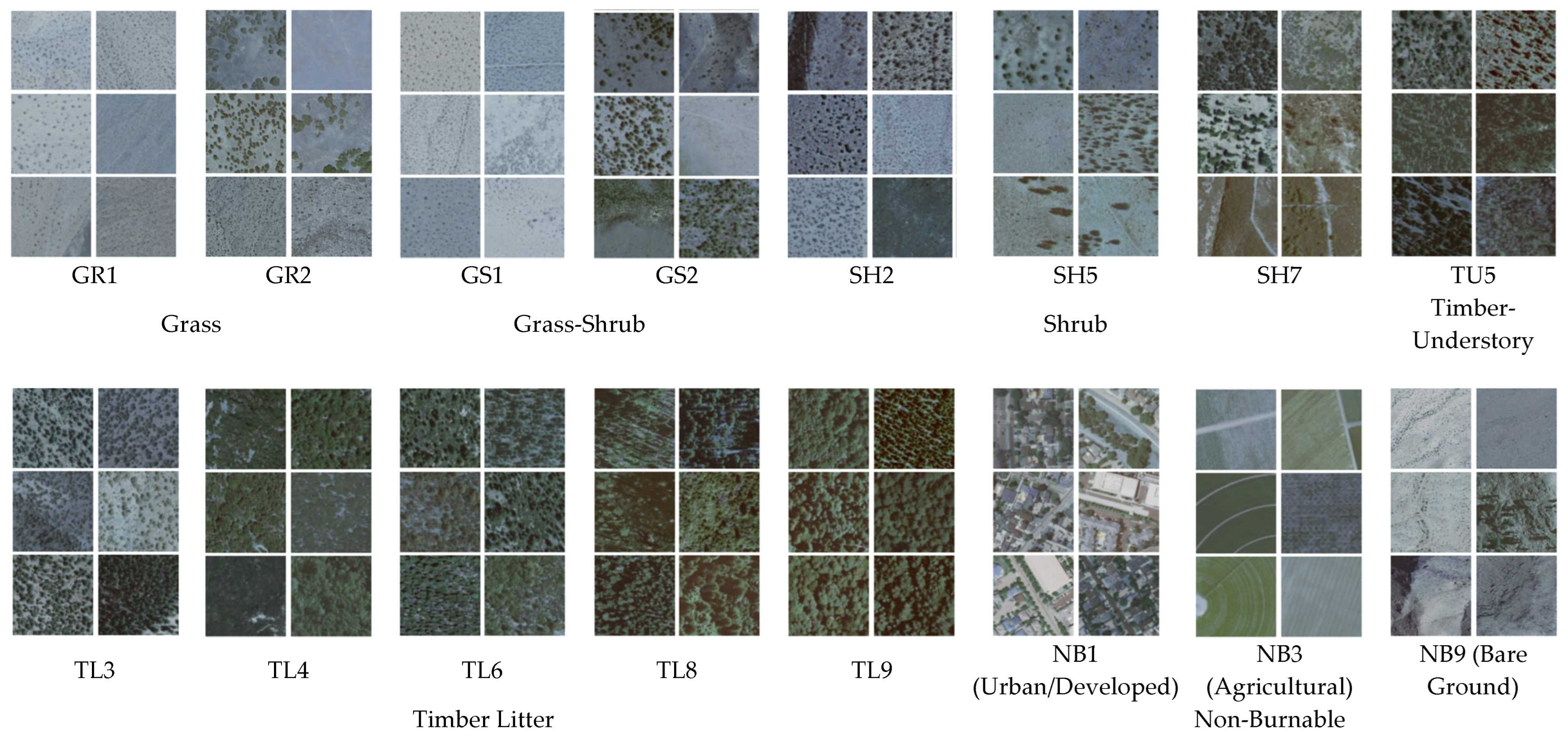Figure 4 depicts sample NAIP images for fuel types under investigation in this study. Of note, Figure 4 shows that some of the fuel types can be difficult to differentiate even for the human eye due to their close visual similarity at the scale under study (e.g., GR1, GR2, and GS1). This depicts the difficulty of the classification task and can foreshadow potential areas of misclassification even by powerful machine learning algorithms. The definitions of the fuel type labels in Figure 4 are based on the Scott and Burgan fuel models [8], and their characteristic differences are presented in Table 2.

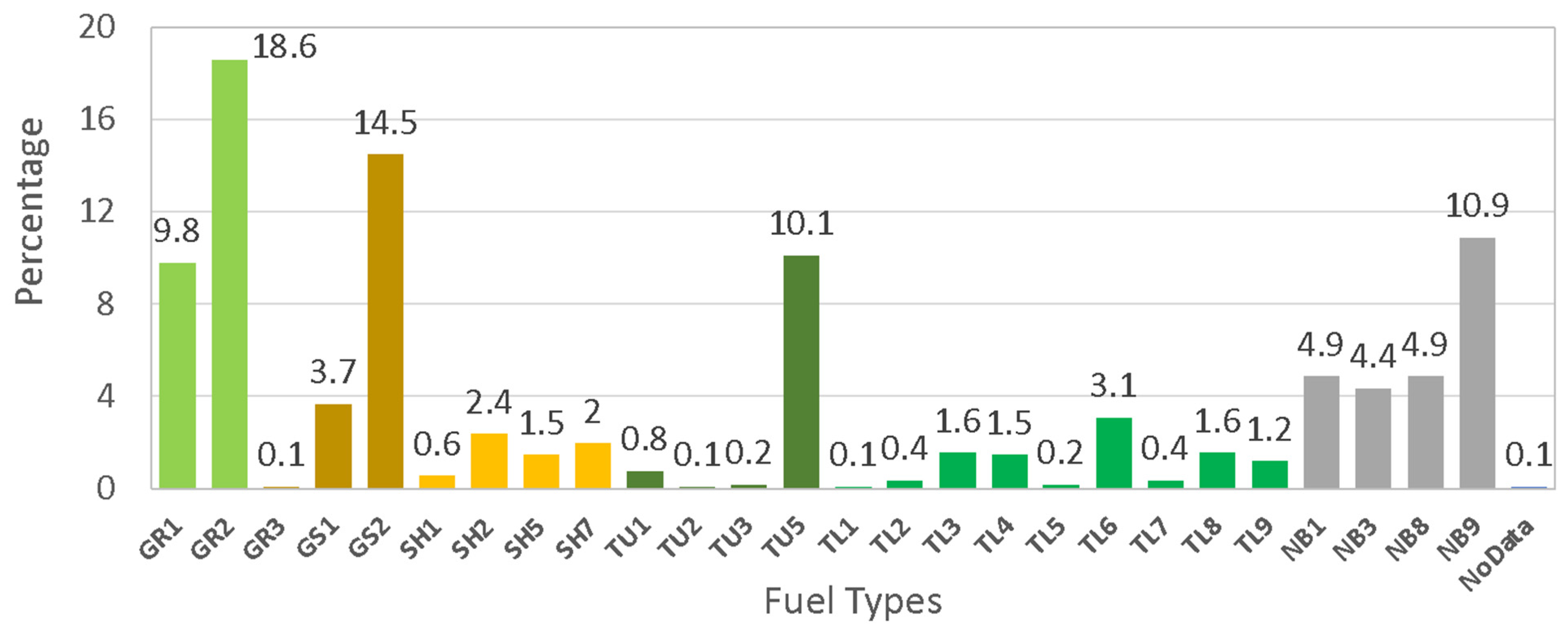
To train the model, ground truth labels describing the fuels found at each location are required. However, large-scale datasets obtained by field surveys that could be used for this purpose are not publicly available (e.g., the Forest Inventory and Analysis (FIA) Database by the United States Forest Service) and fuel model assignments may not be available as part of data collection. To demonstrate the proof of concept and feasibility of training such models, pseudo-labels using an existing fuel map were used in this work. To this end, pseudo-labels for the points of interest were retrieved by randomly sampling fuel pixels from the 2016 LANDFIRE map of standard surface fire behavior fuel models based on Scott and Burgan fuel models. As a result of the random sampling, the distribution of the extracted labels is a function of the frequency of different fuel types across California. Figure 5 depicts a histogram of fuel types for the pixels within the 2016 LANDFIRE fuel map and shows that several fuel types are not widely represented in the fuel map within the area of study. This is important because fuel types with a small frequency of occurrence are known to be difficult for models to learn as a result of the lack of representative data and the resulting imbalance between the classes. On the other hand, mis-predicting a very small number of isolated pixels has a less pronounced effect on the overall fire spread than making errors in the prediction of large areas of dominant fuel types. As a result, identifying the most common fuel types in the study area provides a more important contribution to the effectiveness of the resulting fire spread simulations. Future sensitivity analyses to quantify the effect of individual fuel types—especially rare and small categories—on fire spread modeling are needed to evaluate these effects. To investigate the effects of class size on the fuel identification performance of the model,

Table 5. List and cumulative coverage of fuel types larger than different minimum class sizes. See Table 2 for fuel type descriptions.

Minimum Class Size (% *)	Number of Classes	Cumulative Pixels Covered (% *)	Classes
1%	17	96.5	TL9 (1.2), TL4 (1.5), SH5 (1.5), TL3 (1.5), TL8 (1.5), SH7 (2.0), SH2 (2.4), TL6 (3.1), GS1 (3.7), NB3 (4.4), NB1 (4.9), NB8 (4.9), GR1 (9.8), TU5 (10.1), NB9 (10.9), GS2 (14.5), GR2 (18.6)
2%	12	89.3	SH7 (2.0), SH2 (2.4), TL6 (3.1), GS1 (3.7), NB3 (4.4), NB1 (4.9), NB8 (4.9), GR1 (9.8), TU5 (10.1), NB9 (10.9), GS2 (14.5), GR2 (18.6)
3%	10	84.9	TL6 (3.1), GS1 (3.7), NB3 (4.4), NB1 (4.9), NB8 (4.9), GR1 (9.8), TU5 (10.1), NB9 (10.9), GS2 (14.5), GR2 (18.6)
4%	8	78.1	NB3 (4.4), NB1 (4.9), NB8 (4.9), GR1 (9.8), TU5 (10.1), NB9 (10.9), GS2 (14.5), GR2 (18.6)
5%	5	63.9	GR1 (9.8), TU5 (10.1), NB9 (10.9), GS2 (14.5), GR2 (18.6)

* % of total pixel population.

lists the fuel types larger than different minimum sizes and their cumulative coverages. For example, with a minimum class size of 4%, the model will include 8 classes that cover 78.1% of the pixels of the study area. Alternatively, by aggregating the classes of the same fuel category that are smaller than the minimum class size, models with full coverage of all pixels can be created.

Model Development and Evaluation. This section presents the details of the overall deep learning framework and its design choices previously presented in Figure 2 and Figure 3. Extensive testing was carried out to design the optimal architecture for the proposed model via cross-validation. Pretrained CNN architectures—including VGGNet [30], ResNet [31], DenseNet [32], Inception [33], and InceptionResNet [34]—were tested as the backbone to extract the visual features from the NAIP imagery, and the best accuracy results were achieved using the InceptionResNet_v2 backbone; hence, this architecture was used throughout the rest of the analyses. InceptionResNet_v2 is a 64-layer CNN architecture based on the Inception family of architectures that employs residual connections similar to those in the ResNet variants. The standard implementation of InceptionResNet_v2 available in the Keras library was used in this work, and further information about this architecture can be found in [34]. Input image size was selected to be 128 × 128 pixels, where each pixel represents 1 m on the ground. Data augmentation in the form of random horizontal and vertical flipping and random rotation was applied to the images during training to increase the robustness of the training. Any transformation that could visually change the scene, such as rescaling, recoloring, or non-affine transformations, were not applied, and the original image was maintained during testing. The output of the InceptionResNet_v2 backbone was passed through an average pooling layer that reduces the last convolutional feature map by calculating the average of the feature maps. A dense layer with 128 nodes followed by a dropout layer was added to the end of the CNN branch before concatenation with the multilayer ANN outputs.

A series of DNN hidden layers and node arrangements ranging from 2 to 6 layers and 64 to 256 nodes in increments of 64 were tested to select the configuration that provides the highest accuracy on the validation sets. A substantial increase in the number of layers or nodes did not result in appreciable performance gains. The final configuration of the DNN was determined to include three dense hidden layers each with 128 nodes. Finally, the outputs of the two branches are concatenated with each other and fed to two hidden layers of 128 nodes followed by a softmax classifier (see Figure 1). Softmax is an operator which transforms the outputs from the last layer of a neural network into class probabilities, from which the final classification is decided [70]. Equation (1) shows the softmax operator, where $S_j\left(x\right)$ is the probability of an observation belonging to class j, and n_Class is equal to the number of fuel types under consideration.

$$S_j\left(x\right) = \frac{e^{x_j}}{{\sum }_{l = 1}^{n\_Class}{e}^{x_l}}$$

(1)

A dropout layer with a dropping probability of 0.5 was used after each hidden layer throughout the network to implement the Monte Carlo dropout scheme, as shown in Figure 2. Furthermore, a Rectified Linear Unit (ReLU) activation function in the form of $Re\left(x\right) = \left(0, x\right)$ was used to provide nonlinearity in the neural network that aids the learning of complex patterns. The resulting network was then trained using the Stochastic Gradient Descent (SGD) algorithm [70]. In this process, following every forward pass through the network, training loss is estimated via a cross-entropy loss function. This function is shown in Equation (2), where $y_i$ and ${\widehat{y}}_i$ represent the i-th label and predictions, respectively, and N denotes the size of the training set. The estimated loss in each training epoch is then used in the back-propagation process that updates the unknown parameters (i.e., weights) of the network on small subsets of training data (i.e., mini-batches). In each epoch, the gradients of loss, L, are calculated with respect to the weights, w, ($\frac{\partial L}{\partial w}),$ and a fraction ($\eta$, called learning rate) of the gradient is added to the weights from the previous step ($w^{i - 1})$ (Equations (3) and (4)). To improve the convergence, a term called momentum ($\alpha )$ is added to the update. Finally, another regularization mechanism called weight decay ($\lambda )$ is also used to discourage overfitting by imposing smaller weights [70]. This process is iteratively repeated until convergence.

$$L\left(y_i,{\widehat{y}}_i\right) = - \frac{1}{N}{{\displaystyle \sum }}_i^N{y}_{i}log\left({\widehat{y}}_i\right)$$

(2)

$$∆w^i = \alpha ∆w^{i - 1} + \eta \frac{\partial L}{\partial w} + \lambda \eta w^{i - 1}$$

(3)

$$w^i = w^{i - 1} + ∆w^i$$

(4)

Training of the models was carried out for a maximum of 300 epochs while an early stopping criterion was applied to stop the training if validation accuracy did not improve for 30 consecutive epochs. A minibatch of 100, momentum of 0.9, weight decay of 0.0001, and learning rate of 10⁻³ were used to start training, and the learning rate was reduced by 1/10 after every 15 epochs, following He et al. [31]. Further trial-and-error with these hyperparameters did not provide appreciable accuracy improvements.

The performance of the model was evaluated using well-established classification metrics, including global accuracy, precision, recall, f-score, and Cohen’s Kappa statistic. Global accuracy (Acc) measures the ratio of total correct predictions over the entire data points. Recall (Rec) is the ratio of correct predictions of each fuel type to all predictions of that fuel type. Precision (Pre) is the ratio of correct predictions of each fuel type to all existing labels in that class. F1 score is a widely used metric that is the harmonic mean of precision and recall. Precision, recall, and F1 were computed per class, and both their macro-average (regardless of the size of each class) and their weighted average were calculated. To quantify the agreement between the fuel maps developed through the proposed method with those of LANDFIRE, Cohen’s Kappa statistic was used as a well-established agreement metric in the literature that measures the agreement between predicted and observed labels while accounting for agreement by chance.

The implementation of the deep learning procedures in this paper was carried out using the Keras neural network Application Programming Interface (API) with the TensorFlow deep learning platform as the backend. These platforms provide an array of tools compatible with the Python programming language for designing, developing, and training neural networks [71]. Training of the models was deployed on an NVIDIA Tesla V100 GPU node with 112 GB of RAM.

3. Results

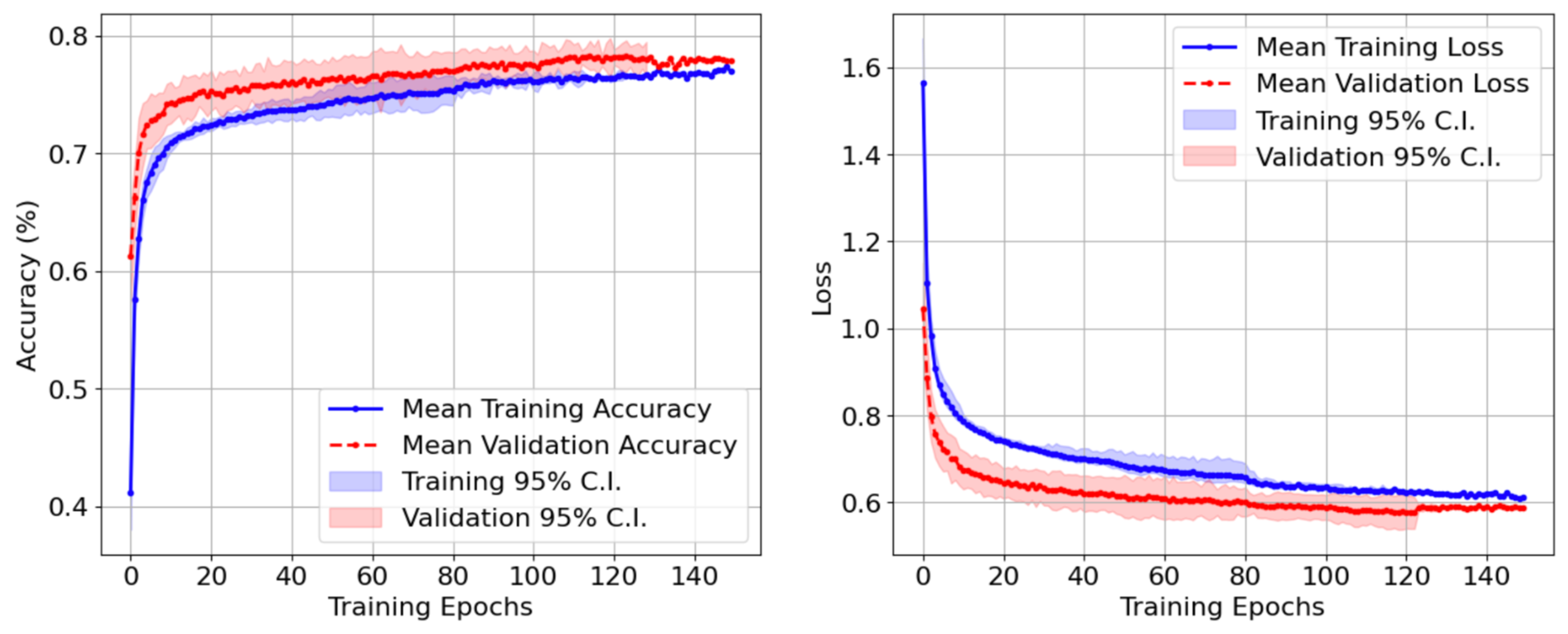
Using the proposed methodology, the models were trained for surface fuel identification. Figure 6 depicts the evolution of training and validation accuracy as well as loss during the training of the model. In this figure, solid lines show the mean of the accuracy and loss for the ensemble, and the shaded band provides the 95% confidence interval. As can be seen in this figure, the model demonstrates stable behavior with the convergence of accuracy and loss to a plateau. Furthermore, the small gap between the training and validation curves in each case demonstrates the proper training of the model with minimal effects of overfitting.

Table 6. Testing accuracy of the model trained both on original unfiltered labels and labels filtered with the National Land Cover Database (NLCD).

Minimum Class Size (% of Total Pixel Population)	Acc (Small Classes Not Aggregated)		Acc (Small Classes Aggregated)
	Unfiltered Labels	Labels Filtered with NLCD	Unfiltered Labels	Labels Filtered with NLCD
1%	51.74	55.62	51.01	52.95
2%	54.08	61.66	52.50	54.94
3%	59.89	64.58	51.17	53.65
4%	67.11	74.31	56.69	59.32
5%	69.59	73.87	57.02	58.17

summarizes the overall accuracy of the model trained using different minimum class sizes ranging from 1–5%. These models were first trained on original unfiltered fuel labels obtained from LANDFIRE 2016 fuel maps, as previously described. The accuracy of the model ranged from 51.74% to 69.59% based on the minimum class size without aggregating the classes smaller than the threshold. The reduction in accuracy with the inclusion of the smaller classes is to be expected, as the model will have less information to learn about the smaller classes. Furthermore, aggregating the small classes with the most similar fuels also results in an accuracy reduction on the order of 10%, which is associated with insufficient information about the small classes as well as possible discrepancies between the aggregated classes. 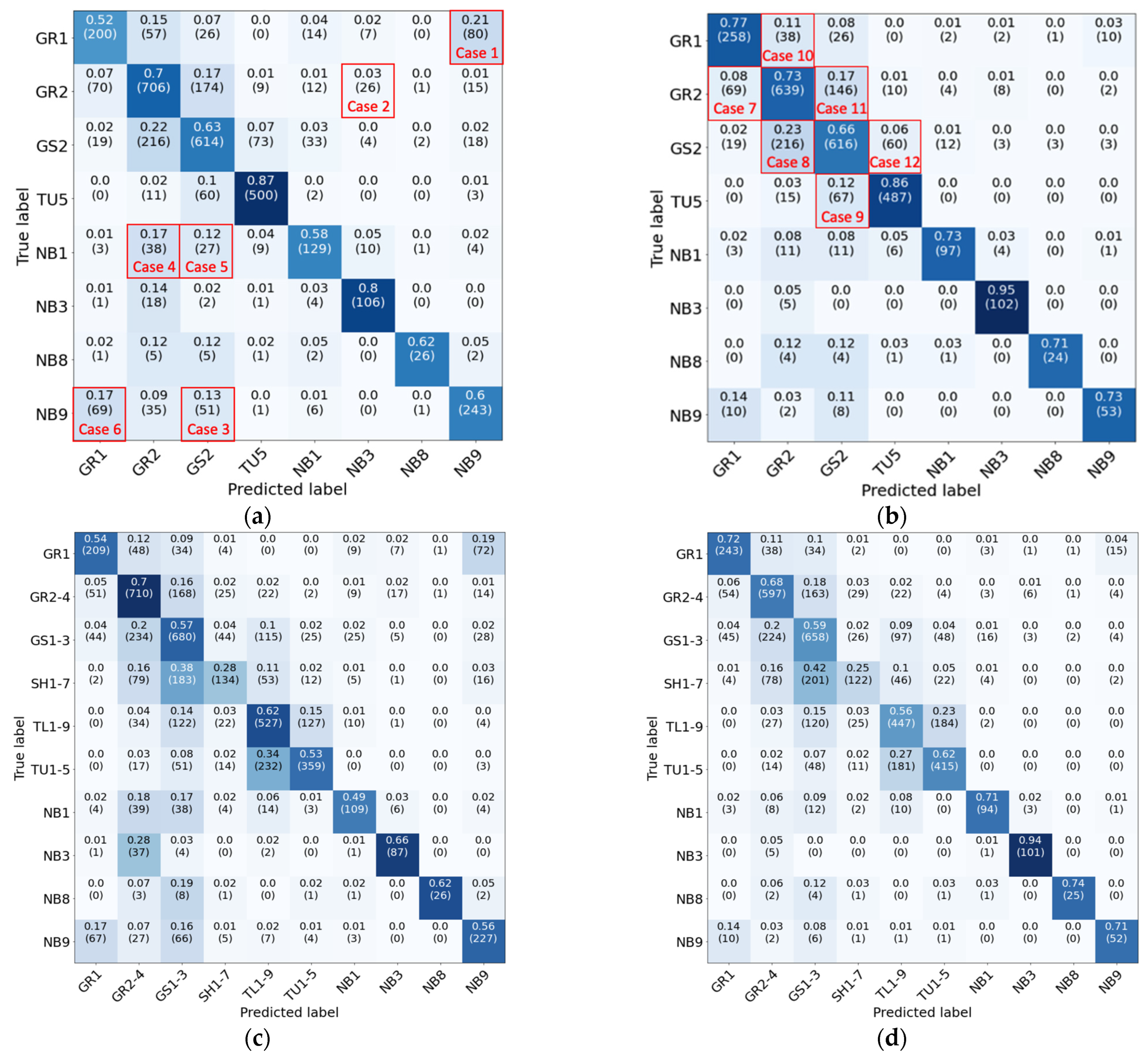For a closer examination of the performance of the system, Figure 7 presents the confusion matrices for the model with a minimum class size of 4%. This case was selected for demonstration as it provides a reasonable accuracy of nearly 70% while covering nearly 80% of the fuel pixels in California.

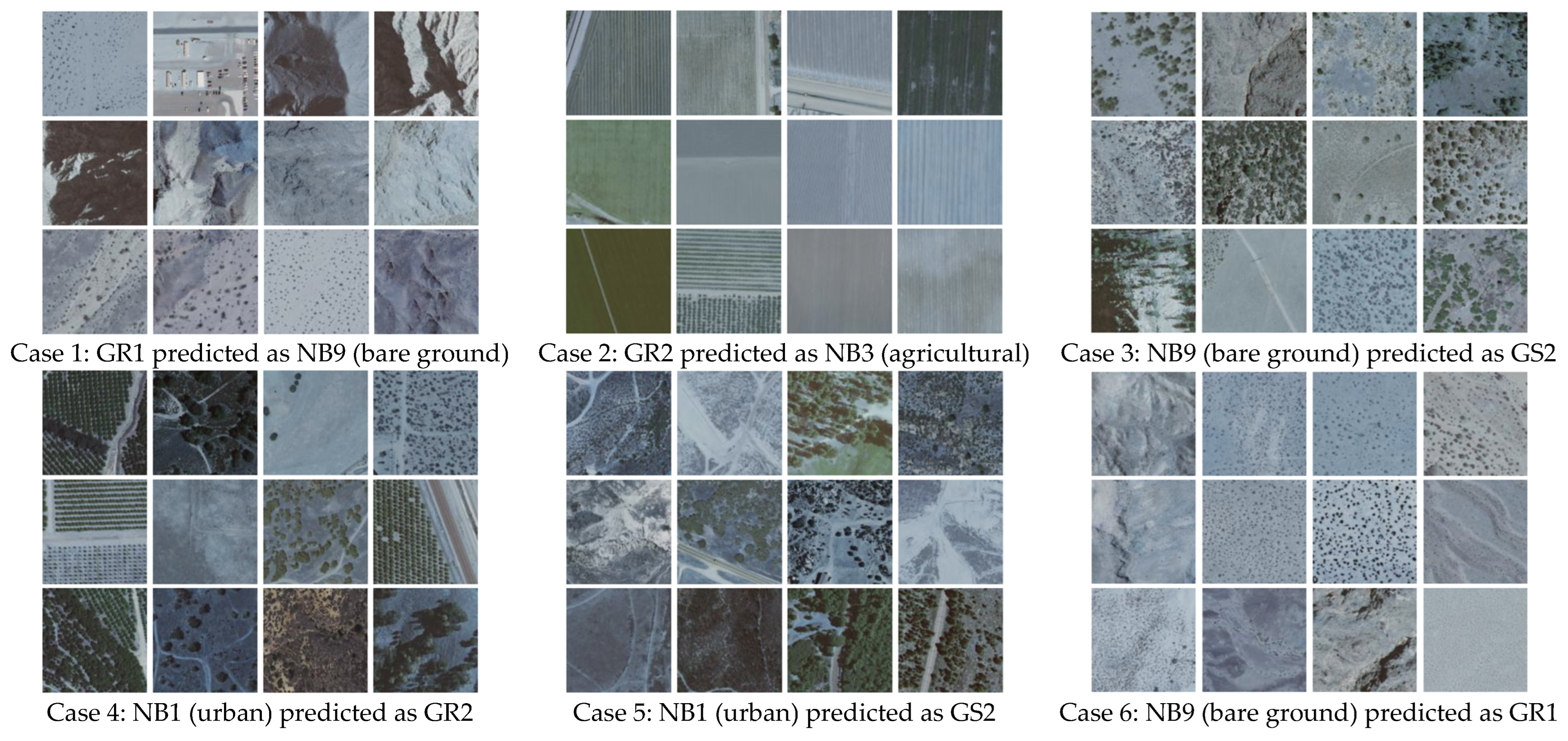
Confusion matrices shown in Figure 7 demonstrate a concentration of the predictions along the diagonal, which shows desirable behavior and noticeable agreement between the predicted fuel labels and the corresponding true labels. To further examine the sources of confusion, in Figure 7a, six cases of misclassification are marked for further visual examination, as presented in Figure 8. In Figure 8, samples of images pertaining to each fuel type that were mistaken for a different fuel type are presented. In each case, the assumed “ground truth” labels show noticeable discrepancies with the contents of the images. For example, Case 2 includes images that are visually consistent with agricultural land cover while they have been labeled as “GR2,” and Case 5 shows mostly non-urban land cover that has been labeled as “urban.” This demonstrates that the labels suffer from a degree of impurity, which can be associated with the fact that these labels are not a direct result of field surveys by fuel experts but are instead sampled from derivative fuel maps, potentially with a level of inherent inaccuracies. Note that agricultural and urban land covers are mapped via external sources ([72,73]) in LANDFIRE [74]. To demonstrate the effect of this label impurity, the models were re-trained after filtering the labels against the National Land Cover Database (NLCD) land cover map for 2016 [73]. Because the NLCD maps do not have fuel information, any burnable fuel pixels that had a non-burnable land cover label were filtered out, and vice versa. These land cover types include developed land (open space and low- to high-intensity development), barren land (rock, clay, and sand), and cultivated crops. This resulted in the removal of 16.3% of the pixels from the training dataset. The results of this filtering are shown in Figure 7b,d, where the severity of the off-diagonal elements has visibly decreased. This resulted in an accuracy improvement of the individual classes by more than 10% on average across all classes and a global accuracy improvement of 7.2% (from 67.11% to 74.31% in Table 6). This demonstrates an important opportunity for the improvement of fuel maps by using the proposed method to detect the discrepancies that can highlight potential label impurities.

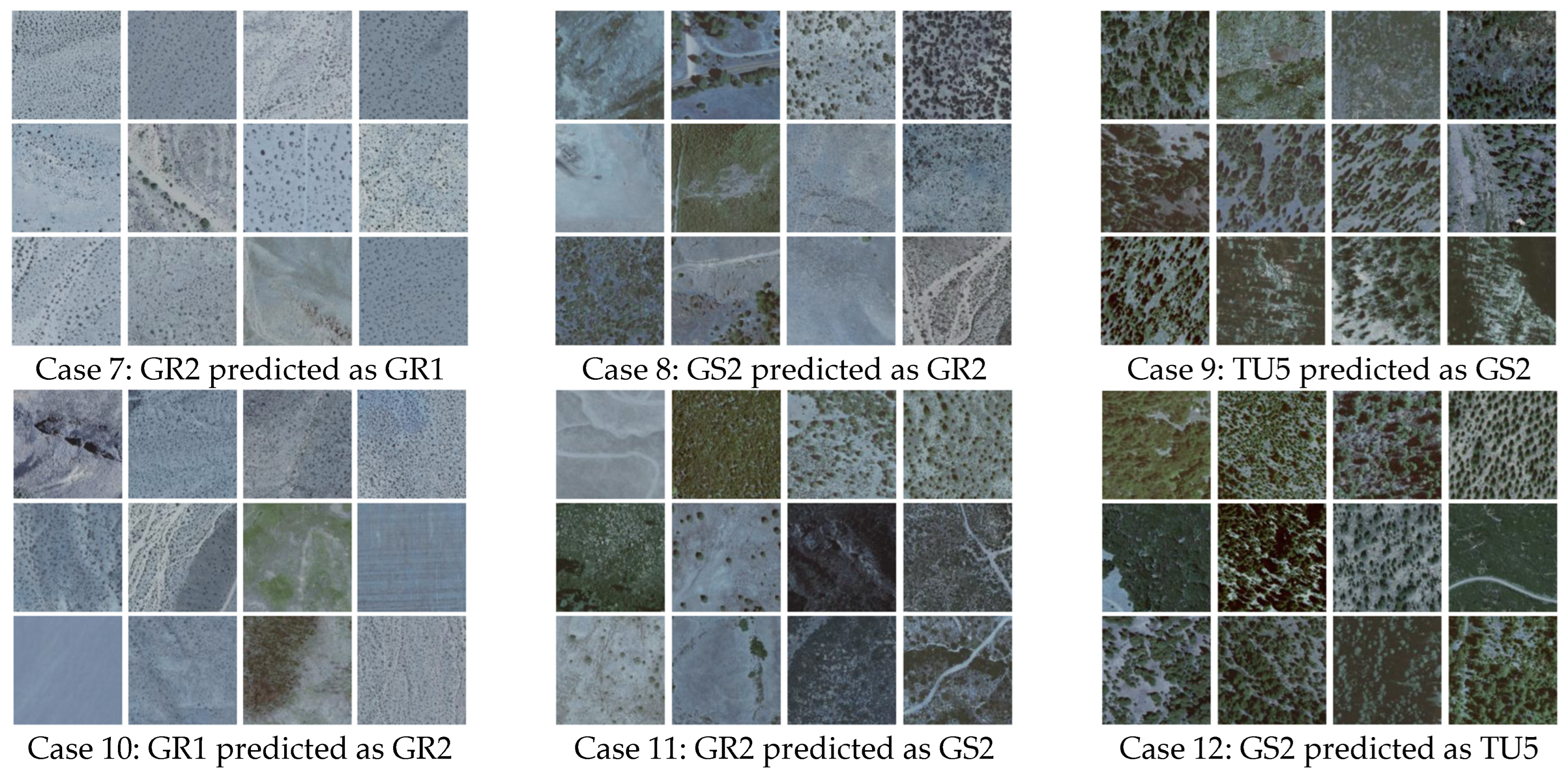
Figure 9 shows six of the biggest off-diagonal confusion elements highlighted in Figure 7b after filtering the labels with the NLCD land cover maps. As can be seen, these cases are mostly concentrated adjacent to the diagonal, which implies that the model’s mistakes are mostly among the most similar fuel types. In Figure 9, each column shows the two fuel types that have been mistaken for each other. Visual inspection of the two cases in each column shows that the differences between these classes are sometimes subtle and can be difficult to differentiate even for human annotators.

Based on the results presented in this section, the evidence suggests that the proposed model is relatively successful at identifying the surface fuel types in the test set given an assumed degree of impurity associated with the labels used for training. The level of fuel identification accuracy is dependent on the desired degree of granularity with smaller minimum class sizes, resulting in learning difficulty with less information to support the extracted patterns. Moreover, based on the confusion matrices in Figure 7b, the non-burnable urban land cover (NB3) is the easiest to detect (class accuracy of 95.3%), which is to be expected, as this class has the most discernible features even to the untrained eye. On the other hand, the grass-shrub class (GS2) is the hardest to detect (class accuracy of 66.1%), which is associated with its close similarity to the grass fuel types.

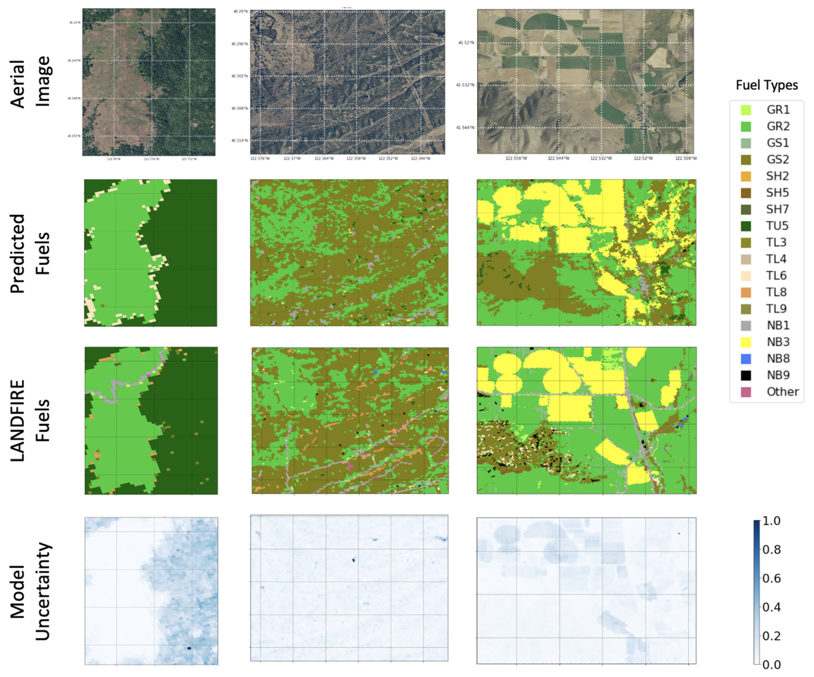
To further visualize the performance of the model outside the testing set and in mapping, Figure 10 and Figure 11 present samples of fuel maps generated by the proposed model together with the corresponding uncertainty maps created as previously described using the average and variance of the model probabilities. As can be seen in Figure 10, the qualitative comparison of the predicted maps with LANDFIRE counterparts shows noticeable overall agreement, consistent with the Cohen’s Kappa values of 0.854, 0.477, and 0.475 for the three images from left to right, respectively. 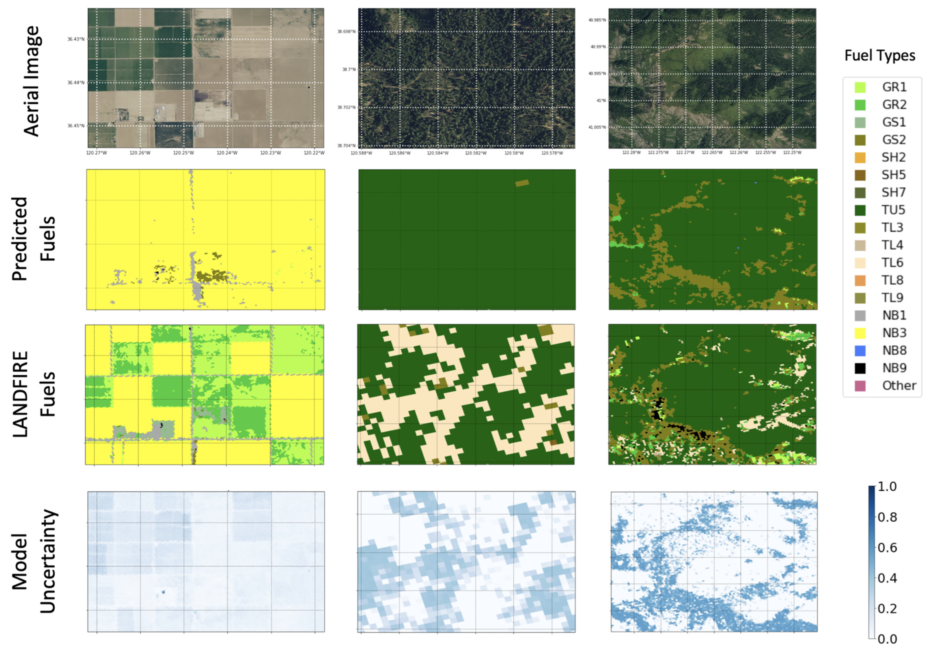Figure 11 shows a sample of results with relatively large discrepancies between the predictions and the target labels, with Cohen’s Kappa values of 0.046, 0.016, and 0.321. Examination of the first column in this figure shows that a large portion of the GR1 and GR2 area in the target map indeed seems to be visually consistent with the predicted NB3 (agricultural). This may be pointing to a potential discrepancy in the target map (i.e., LANDFIRE) that could be used for map correction or improvement. Note that LANDFIRE uses external mapping data for agricultural lands [72]. The second column in this figure shows that the model replaced the area covered by TL6 in the label map with TU5. In this case, the corresponding uncertainty map shows that the model has some awareness of the potentially erroneous prediction that could be accounted for in the resulting decisions. Finally, the third column shows a similar case where, despite the overall relative agreement between the maps, the predictions seem to have missed areas of NB9 (bare ground), TL6, and GR1. Similarly to the previous case, the corresponding uncertainty map may be leveraged to highlight the areas where the model has lower confidence in its predictions.

4. Discussion

Table 7. Performance of different combinations of input components of the model (numbers in the table are F1 scores; values in bold indicate the best result in each category). Fuel types are described in Table 2. M-Avg. and W-Avg. refer to macro- and weighted-average, respectively.

Fuel Class	BP	SV	IM	SI	BP + SI	SV + IM	SI + IM	SI + SV	SV + BP	BP + IM	BP + SI + IM	SV + SI + IM	BP + SI + SV	BP + SV + IM	BP + SI + SV + IM
GR1	67.4	65.5	67.1	64.4	72.4	67.7	67.4	66.8	70.4	71.3	73.6	68.8	72.7	72.8	74.1
GR2	61.9	62.7	65.2	55.5	67.6	66.1	59.2	59.9	66.7	67.2	68.3	65.9	67.1	69.9	70.7
GS2	57.2	65.6	63.2	62.1	65.0	66.4	64.9	64.6	65.7	65.4	67.0	66.6	67.1	67.9	68.1
TU5	73.2	84.4	82.6	82.4	84.0	85.7	84.5	83.9	84.2	83.4	85.1	85.5	84.7	85.2	86.0
NB1	45.4	57.5	75.8	50.5	64.1	76.4	72.3	56.2	67.9	74.2	74.3	75.3	68.4	76.9	77.9
NB3	67.2	70.9	90.4	60.8	78.5	90.4	88.5	75.8	81.8	91.7	90.5	89.7	83.3	90.7	90.3
NB8	40.7	77.4	63.3	66.7	71.2	76.9	72.7	72.4	72.7	67.7	78.7	74.6	78.7	77.6	77.4
NB9	42.6	70.1	56.5	70.1	73.0	72.4	72.7	69.1	67.1	64.3	74.5	72.2	71.5	71.1	75.6
M-Avg.	57.0	69.3	70.5	64.1	72.0	75.3	72.8	68.6	72.1	73.2	76.5	74.8	74.3	76.5	77.4
W-Avg.	62.0	68.3	69.2	63.9	70.8	71.6	68.6	67.3	70.7	71.2	72.9	71.6	72.0	73.6	74.3

SV: spectral values, IM: NAIP imagery, SI: spectral indices, BP: biophysical data.

summarizes the contribution of the different components of the model by listing the per-class and overall F1 scores. As shown in Table 7, in most cases, models made from individual components have the lowest performance, and the fusion of complementary components results in improvements with respect to individual components. Among the individual components, NAIP imagery has the highest overall performance, followed by spectral values. Although the detection of some classes (e.g., NB3, NB1) is substantially easier with imagery than spectral values, others (e.g., NB8, NB9) are easier to differentiate using spectral values. This is associated with how discernible these classes are using their spectral or visual signatures (e.g., agricultural lands may be harder to miss using their unique farm patterns than their spectral differences compared with grasslands). Furthermore, although biophysical data show weak correlations with non-vegetation classes (e.g., NB1, NB8, NB9), they provide the highest performance in the grassland classes. Of note, the addition of imagery data always results in performance improvement. This can be seen by comparing every model (single or multi-component) with its counterpart after the inclusion of imagery data. By comparing the full model with the one that includes all non-imagery data types (SV + SI + BP), all classes except NB8 (water) show accuracy improvement. This lack of improvement for NB8 can be attributed to the apparent visual similarity of some surface water image patches to simple grassland landscapes. Finally, the full model that includes the fusion of all components results in the highest detection performance, both across most individual classes and overall. This demonstrates the benefit of data fusion in improving the fuel identification performance of the system.

Table 8. Effect of stochastic ensemble modeling (values in bold indicate the best result in each category). Fuel classes are described in Table 2. M-Avg. and W-Avg. refer to macro- and weighted-average, respectively.

Fuel Class	Best Single Model			Sub-Sample Ensemble			MC-Dropout Ensemble
	Pre	Rec	F1	Pre	Rec	F1	Pre	Rec	F1
GR1	71.8	65.9	68.7	71.7	74.5	73.1	71.9	76.6	74.1
GR2	65.3	72.7	68.8	68.2	70.7	69.5	68.7	72.8	70.7
GS2	67.6	63.7	65.6	68.8	68.3	68.6	70.2	66.1	68.1
TU5	87.3	80.8	83.9	86.0	85.6	85.8	86.3	85.6	86.0
NB1	75.4	73.7	74.5	80.2	72.9	76.4	83.6	72.9	77.9
NB3	81.4	98.1	89.0	88.4	92.5	90.4	85.7	95.3	90.3
NB8	71.9	67.6	69.7	88.9	70.6	78.7	85.7	70.6	77.4
NB9	65.0	71.2	68.0	90.2	63.0	74.2	76.8	72.6	75.6
M-Avg. (Acc)		71.6		73.8			77.4
W-Avg. (Acc)		71.6		73.9			74.3

compares the performance of the Monte Carlo dropout ensemble with the sub-sample ensemble (without the dropout) and the best individual model. Both ensemble models have higher performances than the best individual model, confirming that the generation of the random ensembles improves predictive performance. Monte Carlo dropout has a slightly higher performance than the sub-sample ensemble in addition to enabling the quantification of fuel identification uncertainty. In Table 8, precision (Pre) and recall (Rec) denote the ratio of correct predictions from each fuel type to all predictions of that fuel type, and to the population of that fuel type, respectively, while the F1 score refers to the harmonic mean of precision and recall.

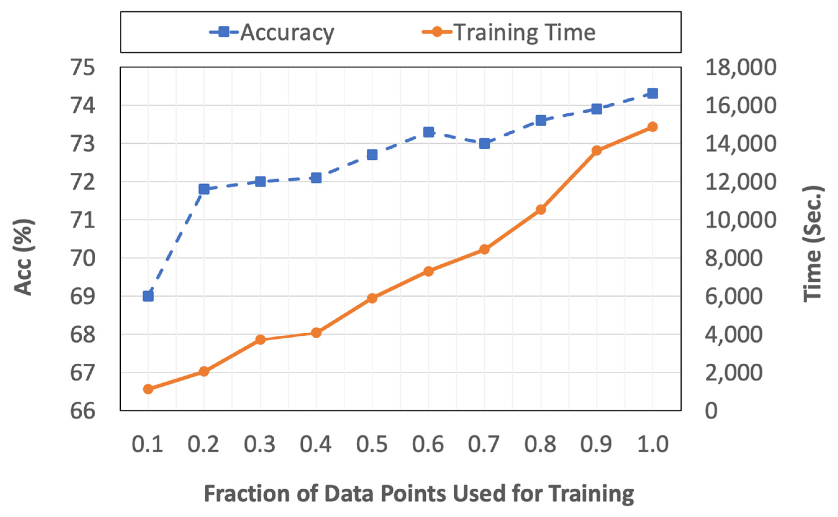
To study the effect of the size of the training set, the proposed model was trained with different fractions of the overall training set population while maintaining the relative size of the classes. Figure 12 summarizes the accuracy of the model as well as its training time for different fractions of the training set size. Based on the figure, increasing the number of data points usually increases the accuracy, but at the cost of increased training time. For example, cutting the training set size in half results in an average of 2.2% and a maximum of 7.2% reduction in per-class accuracies while decreasing the training time from 4.13 to 1.64 h (2.5 times reduction). However, it should be noted that this is a one-time increase during training and that the size of the training set does not affect the computational complexity of the testing and model application if the same model architecture is being used with different training set populations. We also note that the reported training times are based on model deployment on an NVIDIA Tesla V100 GPU node with 112 GB of RAM. The results of this analysis demonstrate that, to create useful large-scale fuel identification models, datasets consisting of tens of thousands of fuel plots may not be required, as the model with 1/10 of the largest data size still achieves an overall accuracy within nearly 5 percent of that with 40,000 observations (Figure 12). The proposed method can also be augmented with semi-supervised learning techniques, such as label propagation, which has been previously used in the remote sensing context to remedy the shortage of ground truth data [75,76].

Finally, to investigate whether the quality of the training set could be improved by avoiding sampling from isolated noisy pixels, a filter was added to the sampling such that only the points with similar fuels within their neighborhood of radius r were selected as training samples. This filter essentially ensures that only the pixels belonging to a relatively homogeneous and continuous body of similar fuel will be sampled, thus reducing the potential noise from the random sampling strategy used. Three different values of r equal to 50, 100, and 150 m were tested. Although some of the individual classes showed small improvements, the overall accuracy of the model slightly decreased with the increase in the radius. This could be attributed to the fact that increasing r resulted in a slight decrease in samples taken from smaller and naturally less prevalent fuel types, thus limiting any potential improvement from the increased sample homogeneity. More generally, enforcing homogeneity by selecting pure sample sites and filtering the minority classes can result in missed opportunities for the identification of natural discontinuities for fuel breaks and other forest management actions. However, the use of survey-based ground truth fuel labels from national data collection campaigns (e.g., FIA database), and large-scale satellite-based lidar measurements (e.g., the Global Ecosystem Dynamics Investigation -GEDI- mission) for canopy fuel modeling can address such limitations by providing high-confidence labels and can be studied in future works.

5. Conclusions

Most past wildfire surface fuel mapping studies proposed models trained for and applicable to small areas of interest. In contrast, this paper discussed a model for creating large-scale wildfire surface fuel mapping models that can be applied at regional (e.g., state) scales. The proposed model takes advantage of deep learning to create a predictive model that can fuse information from spectral, biophysical, and high-resolution imagery. The model also features a stochastic ensemble approach using the Monte Carlo dropout technique, which both improves the performance of the model and produces a measure of model uncertainty for the predicted fuels.

The proposed system was applied to a dataset that was compiled using a random sample of the 2016 LANDFIRE surface fuel product based on the Scott and Burgan 40 fuel models for the state of California as the target fuel labels. The results demonstrated the feasibility of the proposed approach that yielded approximately 55% to 75% accuracy, depending on the desired smallest fuel type size to be included in the model. A considerable portion of the error is attributed to the close visual similarity of some of the fuel types at the scales under study, as evidenced by the difficulty of differentiating them even through human examination. In this regard, the proposed model can thus be used to reveal areas of potential discrepancies and high uncertainty in existing fuel maps and to interpolate fuel distributions for points of interest in time. Although the effect of minimum class size included in the model on the fuel identification accuracy was studied and showed an anticipated decrease in the model’s performance when including very small classes, its cascading effect on the performance of the resulting fire spread simulations was outside the scope of this study and is deferred to a future study that could compare the predicted fire spread parameters with different fuel identification models.

Analysis of the properties of the proposed system revealed that the fusion of different types of data improves identification accuracy compared to using each data source individually. Specifically, the addition of high-resolution imagery from the NAIP program to any of the models from individual or combined data sources always improved their fuel identification performance. Furthermore, the proposed stochastic model ensemble generation approach resulted in improved performance with respect to individual models while allowing for the generation of model uncertainty estimates that could be propagated throughout resulting fire spread simulations. This can in turn enable uncertainty-aware scenario-based decision-making and model updating. A study of the effect of the size of the training set on the performance of the model revealed an increase in accuracy with an increase in the training set size. Namely, cutting the training set in half resulted in a maximum reduction of 7.2% and an average reduction of 2.2% in per-class performance, while cutting the training time by 2.5 times. This implies that the model has the capacity to benefit from an increased training set (i.e., more data), considering that the training of even the largest model was relatively manageable given the hardware used in this study (overall training of the ensemble model took approximately 4 h).

This proof-of-concept study used a random geospatial sampling of existing LANDFIRE fuel products to extract target labels for training. However, the proposed approach is generic and can be applied to collections of field data resulting from in situ fuel plots. Although the reviewed literature has successfully used small collections of field plots from site-specific campaigns to create fuel identification models, large-scale state- or nationwide fuel identification models can be created using the proposed approach and national data collection campaigns such as the Forest Inventory and Analysis (FIA) program of the United States Forest Service. Furthermore—with fire behavior fuel models being classification systems that use simplifying assumptions that limit their capability to capture the full variation of fuels—the development of quantitative, physics-based fuel models that more accurately characterize the combustible biomass would be beneficial. The success of the proposed approach in creating large-scale models that can describe fuels illuminates a promising pathway for creating such models, given access to in situ biomass measurement data from national programs. This approach could be used to create the real-time on-demand capability for updating fuel maps. Finally, an underlying limitation of the proposed approach is the limited ability of the optical remote sensing data sources (Landsat multispectral and NAIP imagery) to capture information about the understory layers covered by dense canopies, or to provide information about the height of the understory vegetation. Similarly to most of the previous works in the literature, this work attempted to leverage latent and indirect relationships between understory conditions and those from the uppermost canopy layers that are more readily discernible in optical remote sensing data. However, unlike some of the recent work in vegetation and fuel mapping, the use of lidar data was not possible due to the lack of consistent state-wide coverage for the given period of time. With the future introduction of large-scale yet high-resolution lidar sensors, the proposed approach could be extended to allow for the fusion of the resulting spatial data into the fuel identification model.

References

1. National Interagency Fire Center. Fire Information and Statistics. Available online: https://www.nifc.gov/fireInfo/fireInfo_statistics.html (accessed on 1 March 2022).
2. Iglesias, V.; Balch, J.K.; Travis, W.R. U.S. Fires Became Larger, More Frequent, and More Widespread in the 2000s. 2022. Available online: https://www.science.org (accessed on 1 September 2022).
3. United Nations. Spreading Like Wildfire: The Rising Threat of Extraordinary Landscape Fires. 2022. Available online: http://www.un.org/Depts/ (accessed on 1 March 2022).
4. Kalabokidis, K.; Ager, A.; Finney, M.; Athanasis, N.; Palaiologou, P.; Vasilakos, C. AEGIS: A wildfire prevention and management information system. Nat. Hazards Earth Syst. Sci. 2016, 16, 643–661. [Google Scholar] [CrossRef] [Green Version]
5. Sakellariou, S.; Tampekis, S.; Samara, F.; Sfougaris, A.; Christopoulou, O. Review of state-of-the-art decision support systems (DSSs) for prevention and suppression of forest fires. J. For. Res. 2017, 28, 1107–1117, Northeast Forestry University. [Google Scholar] [CrossRef]
6. Keane, R.E. Wildland Fuel Fundamentals and Applications; Springer International Publishing: New York, NY, USA, 2015. [Google Scholar] [CrossRef]
7. Anderson, H.E. Aids to Determining Fuel Models for Estimating Fire Behavior; USDA Forest Service: Ogden, UT, USA, 1982; pp. 1–22. [Google Scholar] [CrossRef] [Green Version]
8. Scott, J.H.; Burgan, R.E. Standard Fire Behavior Fuel Models: A Comprehensive Set for Use with Rothermel’s Surface Fire Spread Model; U.S. Department of Agriculture, Forest Service, Rocky Mountain Research Station: Fort Collins, CO, USA, 2005; p. 153. [Google Scholar] [CrossRef]
9. Rowell, E.; Loudermilk, E.L.; Seielstad, C.; O’Brien, J.J. Using Simulated 3D Surface Fuelbeds and Terrestrial Laser Scan Data to Develop Inputs to Fire Behavior Models. Can. J. Remote Sens. 2016, 42, 443–459. [Google Scholar] [CrossRef]
10. Rollins, M.G. LANDFIRE: A nationally consistent vegetation, wildland fire, and fuel assessment. Int. J. Wildland Fire 2009, 18, 235–249. [Google Scholar] [CrossRef] [Green Version]
11. Keane, R.E.; Reeves, M. Use of Expert Knowledge to Develop Fuel Maps for Wildland Fire Management. In Expert Knowledge and its Application in Landscape Ecology; Springer: New York, NY, USA, 2012; Volume 9781461410348, pp. 211–228. [Google Scholar] [CrossRef]
12. Pickell, P.D.; Chavardes, R.D.; Li, S.; Daniels, L.D. FuelNet: An Artificial Neural Network for Learning and Updating Fuel Types for Fire Research. IEEE Trans. Geosci. Remote Sens. 2020, 59, 7338–7352. [Google Scholar] [CrossRef]
13. Stavros, E.N.; Coen, J.; Peterson, B.; Singh, H.; Kennedy, K.; Ramirez, C.; Schimel, D. Use of imaging spectroscopy and LIDAR to characterize fuels for fire behavior prediction. Remote Sens. Appl. Soc. Environ. 2018, 11, 41–50. [Google Scholar] [CrossRef]
14. Benito, A.A.; Arroyo, L.A.; Arbelo, M.; Hernández-Leal, P.; Gonzalez-Calvo, A. Pixel and object-based classification approaches for mapping forest fuel types in Tenerife Island from ASTER data. Int. J. Wildland Fire 2013, 22, 306–317. [Google Scholar] [CrossRef]
15. Chirici, G.; Scotti, R.; Montaghi, A.; Barbati, A.; Cartisano, R.; Lopez, G.; Marchetti, M.; McRoberts, R.E.; Olsson, H.; Corona, P. Stochastic gradient boosting classification trees for forest fuel types mapping through airborne laser scanning and IRS LISS-III imagery. Int. J. Appl. Earth Obs. Geoinf. 2013, 25, 87–97. [Google Scholar] [CrossRef] [Green Version]
16. Huesca, M.; Riaño, D.; Ustin, S.L. Spectral mapping methods applied to LiDAR data: Application to fuel type mapping. Int. J. Appl. Earth Obs. Geoinf. 2019, 74, 159–168. [Google Scholar] [CrossRef] [Green Version]
17. Lasaponara, R.; Lanorte, A. Remotely sensed characterization of forest fuel types by using satellite ASTER data. Int. J. Appl. Earth Obs. Geoinf. 2007, 9, 225–234. [Google Scholar] [CrossRef]
18. Jakubowksi, M.K.; Guo, Q.; Collins, B.; Stephens, S.; Kelly, M. Predicting Surface Fuel Models and Fuel Metrics Using Lidar and CIR Imagery in a Dense, Mountainous Forest. Photogramm. Eng. Remote Sens. 2013, 79, 37–49. [Google Scholar] [CrossRef] [Green Version]
19. García, M.; Riaño, D.; Chuvieco, E.; Salas, J.; Danson, F. Multispectral and LiDAR data fusion for fuel type mapping using Support Vector Machine and decision rules. Remote Sens. Environ. 2011, 115, 1369–1379. [Google Scholar] [CrossRef]
20. Mutlu, M.; Popescu, S.C.; Stripling, C.; Spencer, T. Mapping surface fuel models using lidar and multispectral data fusion for fire behavior. Remote Sens. Environ. 2008, 112, 274–285. [Google Scholar] [CrossRef]
21. Marino, E.; Ranz, P.; Tomé, J.L.; Noriega, M.; Esteban, J.; Madrigal, J. Generation of high-resolution fuel model maps from discrete airborne laser scanner and Landsat-8 OLI: A low-cost and highly updated methodology for large areas. Remote Sens. Environ. 2016, 187, 267–280. [Google Scholar] [CrossRef]
22. Riano, D.; Chuvieco, E.; Salas, J.; Orueta, A.P.; Bastarrika, A. Generation of fuel type maps from Landsat TM images and ancillary data in Mediterranean ecosystems. Can. J. For. Res. 2002, 32, 1301–1315. [Google Scholar] [CrossRef]
23. Alonso-Benito, A.; Arroyo, L.A.; Arbelo, M.; Hernández-Leal, P. Fusion of WorldView-2 and LiDAR Data to Map Fuel Types in the Canary Islands. Remote Sens. 2016, 8, 669. [Google Scholar] [CrossRef]
24. Domingo, D.; Domingo, D.; de la Riva, J.; de la Riva, J.; Lamelas, M.; Lamelas, M.; García-Martín, A.; García-Martín, A.; Ibarra, P.; Ibarra, P.; et al. Fuel Type Classification Using Airborne Laser Scanning and Sentinel 2 Data in Mediterranean Forest Affected by Wildfires. Remote Sens. 2020, 12, 3660. [Google Scholar] [CrossRef]
25. Krasnow, K.; Schoennagel, T.; Veblen, T.T. Forest fuel mapping and evaluation of LANDFIRE fuel maps in Boulder County, Colorado, USA. For. Ecol. Manag. 2009, 257, 1603–1612. [Google Scholar] [CrossRef]
26. Falkowski, M.J.; Gessler, P.E.; Morgan, P.; Hudak, A.T.; Smith, A. Characterizing and mapping forest fire fuels using ASTER imagery and gradient modeling. For. Ecol. Manag. 2005, 217, 129–146. [Google Scholar] [CrossRef] [Green Version]
27. Mallinis, G.; Galidaki, G.; Gitas, I. A Comparative Analysis of EO-1 Hyperion, Quickbird and Landsat TM Imagery for Fuel Type Mapping of a Typical Mediterranean Landscape. Remote Sens. 2014, 6, 1684–1704. [Google Scholar] [CrossRef] [Green Version]
28. Riley, K.; Thompson, M. An Uncertainty Analysis of Wildfire Modeling. In Natural Hazard Uncertainty Assessment: Modeling and Decision Support; Wiley: Hoboken, NJ, USA, 2016; pp. 193–213. [Google Scholar] [CrossRef]
29. Bechtold, W.A.; Patterson, P.L. The Enhanced Forest Inventory and Analysis Program-National Sampling Design and Estimation Procedures; USDA Forest Service, Southern Research Station: Asheville, NC, USA, 2005. [Google Scholar]
30. Simonyan, K.; Zisserman, A. Very deep convolutional networks for large-scale image recognition. In Proceedings of the 3rd International Conference on Learning Representations, ICLR 2015, San Diego, CA, USA, 7–9 May 2015; Available online: https://arxiv.org/abs/1409.1556 (accessed on 1 February 2022).
31. He, K.; Zhang, X.; Ren, S.; Sun, J. Deep residual learning for image recognition. In Proceedings of the IEEE Computer Society Conference on Computer Vision and Pattern Recognition (CVPR), Las Vegas, NV, USA, 27–30 June 2016; pp. 770–778. [Google Scholar] [CrossRef] [Green Version]
32. Huang, G.; Liu, Z.; van der Maaten, L.; Weinberger, K.Q. Densely Connected Convolutional Networks. 2016. Available online: http://arxiv.org/abs/1608.06993 (accessed on 1 March 2022).
33. Szegedy, C.; Vanhoucke, V.; Ioffe, S.; Shlens, J. Rethinking the Inception architecture for computer vision. In Proceedings of the IEEE Conference on Computer Vision and Pattern Recognition, Las Vegas, NV, USA, 27–30 June 2016; pp. 2818–2826. [Google Scholar]
34. Szegedy, C.; Ioffe, S.; Vanhoucke, V.; Alemi, A. Inception-v4, Inception-ResNet and the Impact of Residual Connections on Learning. In Proceedings of the 31st AAAI Conference on Artificial Intelligence, San Francisco, CA, USA, 4–9 February 2017. [Google Scholar]
35. Kattenborn, T.; Leitloff, J.; Schiefer, F.; Hinz, S. Review on Convolutional Neural Networks (CNN) in vegetation remote sensing. ISPRS J. Photogramm. Remote Sens. 2021, 173, 24–49. [Google Scholar] [CrossRef]
36. Yosinski, J.; Clune, J.; Bengio, Y.; Lipson, H. How transferable are features in deep neural networks? In Proceedings of the Advances in Neural Information Processing Systems, Montreal, QC, Canada, 8–13 December 2014.
37. Zhuang, F.; Qi, Z.; Duan, K.; Xi, D.; Zhu, Y.; Zhu, H.; Xiong, H.; He, Q. A Comprehensive Survey on Transfer Learning. Proc. IEEE 2021, 109, 43–76. [Google Scholar] [CrossRef]
38. Hu, F.; Xia, G.-S.; Hu, J.; Zhang, L. Transferring Deep Convolutional Neural Networks for the Scene Classification of High-Resolution Remote Sensing Imagery. Remote Sens. 2015, 7, 14680–14707. [Google Scholar] [CrossRef] [Green Version]
39. Pires de Lima, R.; Marfurt, K. Convolutional Neural Network for Remote-Sensing Scene Classification: Transfer Learning Analysis. Remote Sens. 2019, 12, 86. [Google Scholar] [CrossRef]
40. Castelluccio, M.; Poggi, G.; Sansone, C.; Verdoliva, L. Land Use Classification in Remote Sensing Images by Convolutional Neural Networks. 2015. Available online: http://arxiv.org/abs/1508.00092 (accessed on 1 March 2022).
41. Deng, J.; Dong, W.; Socher, R.; Li, L.-J.; Li, K.; Fei-Fei, L. ImageNet: A large-scale hierarchical image database. In Proceedings of the 2009 IEEE Conference on Computer Vision and Pattern Recognition, Miami, FL, USA, 20–25 June 2009; pp. 248–255. [Google Scholar] [CrossRef] [Green Version]
42. Belkin, M.; Hsu, D.; Ma, S.; Mandal, S. Reconciling modern machine-learning practice and the classical bias–variance trade-off. Proc. Natl. Acad. Sci. USA 2019, 116, 15849–15854. [Google Scholar] [CrossRef] [Green Version]
43. Gal, Y.; Ghahramani, Z. Dropout as a Bayesian approximation: Representing model uncertainty in deep learning. In Proceedings of the International Conference on Machine Learning, New York, NY, USA, 19–24 June 2016; pp. 1050–1059, PMLR. [Google Scholar]
44. Srivastava, N.; Hinton, G.; Krizhevsky, A.; Salakhutdinov, R. Dropout: A simple way to prevent neural networks from overfitting. J. Mach. Learn. Res. 2014, 15, 1929–1958. [Google Scholar]
45. Kendall, A.; Badrinarayanan, V.; Cipolla, R. Bayesian SegNet: Model Uncertainty in Deep Convolutional Encoder-Decoder Architectures for Scene Understanding. arXiv 2015, arXiv:1511.02680. [Google Scholar]
46. Abdar, M.; Salari, S.; Qahremani, S.; Lam, H.K.; Karray, F.; Hussain, S.; Khosravi, A.; Acharya, U.R.; Makarenkov, V.; Nahavandi, S. UncertaintyFuseNet: Robust Uncertainty-Aware Hierarchical Feature Fusion model with Ensemble Monte Carlo Dropout for COVID-19 Detection. 2021. Available online: http://arxiv.org/abs/2105.08590 (accessed on 1 March 2022).
47. Sadr, M.A.M.; Gante, J.; Champagne, B.; Falcao, G.; Sousa, L. Uncertainty Estimation via Monte Carlo Dropout in CNN-Based mmWave MIMO Localization. IEEE Signal Process. Lett. 2021, 29, 269–273. [Google Scholar] [CrossRef]
48. Haas, J.; Rabus, B. Uncertainty Estimation for Deep Learning-Based Segmentation of Roads in Synthetic Aperture Radar Imagery. Remote Sens. 2021, 13, 1472. [Google Scholar] [CrossRef]
49. Nardelli, B.B. A Deep Learning Network to Retrieve Ocean Hydrographic Profiles from Combined Satellite and In Situ Measurements. Remote Sens. 2020, 12, 3151. [Google Scholar] [CrossRef]
50. Myojin, T.; Hashimoto, S.; Mori, K.; Sugawara, K.; Ishihama, N. Improving Reliability of Object Detection for Lunar Craters Using Monte Carlo Dropout. In Proceedings of the International Conference on Artificial Intelligence, Munich, Germany, 17–19 September 2019. [Google Scholar]
51. Dechesne, C.; Lassalle, P.; Lefèvre, S. Bayesian U-Net: Estimating Uncertainty in Semantic Segmentation of Earth Observation Images. Remote Sens. 2021, 13, 3836. [Google Scholar] [CrossRef]
52. Zhu, Z.; Wulder, M.A.; Roy, D.P.; Woodcock, C.E.; Hansen, M.C.; Radeloff, V.C.; Healey, S.P.; Schaaf, C.; Hostert, P.; Strobl, P.; et al. Benefits of the free and open Landsat data policy. Remote. Sens. Environ. 2019, 224, 382–385. [Google Scholar] [CrossRef]
53. Flood, N. Seasonal Composite Landsat TM/ETM+ Images Using the Medoid (a Multi-Dimensional Median). Remote Sens. 2013, 5, 6481–6500. [Google Scholar] [CrossRef] [Green Version]
54. Van Doninck, J.; Tuomisto, H. A Landsat composite covering all Amazonia for applications in ecology and conservation. Remote Sens. Ecol. Conserv. 2018, 4, 197–210. [Google Scholar] [CrossRef] [Green Version]
55. Gesch, D.; Oimoen, M.; Greenlee, S.; Nelson, C.; Steuck, M.; Tyler, D. The National Elevation Dataset. Photogramm. Eng. Remote Sens. 2002, 68, 5–32. [Google Scholar]
56. O. S. U. PRISM Climate Group; PRISM Climate Group; Oregon State University. 2004. Available online: https://prism.oregonstate.edu (accessed on 1 March 2022).
57. NAIP (National Agricultural Imagery Program). U.S. Department of Agriculture Farm Service Agency. 2016. Available online: https://www.fsa.usda.gov/programs-and-services/aerial-photography/imagery-programs/naip-imagery/index (accessed on 20 February 2022).
58. Theobald, D.M.; Harrison-Atlas, D.; Monahan, W.B.; Albano, C.M. Ecologically-Relevant Maps of Landforms and Physiographic Diversity for Climate Adaptation Planning. PLoS ONE 2015, 10, e0143619. [Google Scholar] [CrossRef]
59. Rouse, R.W.H.; Haas, J.; Deering, D.W. Monitoring vegetation systems in the Great Plains with ERTS-1. In Proceedings of the 3rd Earth Resources Technology Satellite Symposium, Washington, DC, USA, 10–14 December 1973. [Google Scholar]
60. Huete, A.; Didan, K.; Miura, T.; Rodriguez, E.P.; Gao, X.; Ferreira, L.G. Overview of the radiometric and biophysical performance of the MODIS vegetation indices. Remote Sens. Environ. 2002, 83, 195–213. [Google Scholar] [CrossRef]
61. Huete, A.R. A soil-adjusted vegetation index (SAVI). Remote Sens. Environ. 1988, 25, 295–309. [Google Scholar] [CrossRef]
62. Qi, J.; Chehbouni, A.; Huete, A.R.; Kerr, Y.H.; Sorooshian, S. A modified soil adjusted vegetation index. Remote Sens. Environ. 1994, 48, 119–126. [Google Scholar] [CrossRef]
63. Gao, B.-C. Normalized Difference Water Index for Remote Sensing of Vegetation Liquid Water from Space. In Proceedings of the SPIE’S 1995 Symposium on OE/Aerospace Sensing and Dual Use Photonics, Orlando, FL, USA, 17–21 April 1995; pp. 225–236. [Google Scholar] [CrossRef]
64. Kauth, R.J.; Thomas, G.S. Tasselled Cap-A Graphic Description of the Spectral-Temporal Development of Agricultural Crops as Seen by Landsat. 1976. Available online: http://docs.lib.purdue.edu/lars_symphttp://docs.lib.purdue.edu/lars_symp/159 (accessed on 1 March 2022).
65. Gitelson, A.A.; Kaufman, Y.J.; Stark, R.; Rundquist, D. Novel algorithms for remote estimation of vegetation fraction. Remote Sens. Environ. 2002, 80, 76–87. [Google Scholar] [CrossRef] [Green Version]
66. López-García, M.J.; Caselles, V. Mapping burns and natural reforestation using thematic Mapper data. Geocarto Int. 1991, 6, 31–37. [Google Scholar] [CrossRef]
67. Landsat Missions. Landsat Enhanced Vegetation Index. Available online: https://www.usgs.gov/landsat-missions/landsat-enhanced-vegetation-index (accessed on 10 December 2021).
68. U.S. Geological Survey. Landsat Soil Adjusted Vegetation Index. Available online: https://www.usgs.gov/landsat-missions/landsat-soil-adjusted-vegetation-index (accessed on 12 April 2022).
69. DeVries, B.; Pratihast, A.K.; Verbesselt, J.; Kooistra, L.; Herold, M. Characterizing Forest Change Using Community-Based Monitoring Data and Landsat Time Series. PLoS ONE 2016, 11, e0147121. [Google Scholar] [CrossRef] [PubMed]
70. Goodfellow, I.; Bengio, Y.; Courville, A. Deep Learning; MIT Press: Cambridge, MA, USA, 2016. [Google Scholar]
71. Chollet, F. Keras. 2015. Available online: https://keras.io (accessed on 1 March 2022).
72. California Department of Water Resources. Statewide Crop Mapping Dataset; California Department of Water Resources Land Use Program: Sacramento, CA, USA, 2017. [Google Scholar]
73. Multi-Resolution Land Characteristics (MRLC) Consortium. Available online: https://www.mrlc.gov/ (accessed on 1 March 2022).
74. La Puma, I.; Deis, J.; Soluk, E.; Hatten, T.; Lundberg, B.; Tolk, B.; Picotte, J.; Kumar, S.; Dockter, D.; Degaga, E.; et al. LANDFIRE Technical Documentation; U.S. Geological Survey, Earth Resources and Observation Science Center: Sioux Falls, SD, USA, 2022. [Google Scholar]
75. Hao, F.; Ma, Z.-F.; Tian, H.-P.; Wang, H.; Wu, D. Semi-supervised label propagation for multi-source remote sensing image change detection. Comput. Geosci. 2023, 170, 105249. [Google Scholar] [CrossRef]
76. Cui, B.; Xie, X.; Hao, S.; Cui, J.; Lu, Y. Semi-Supervised Classification of Hyperspectral Images Based on Extended Label Propagation and Rolling Guidance Filtering. Remote Sens. 2018, 10, 515. [Google Scholar] [CrossRef]
Figure 1. Proposed deep learning-based surface fuel identification framework (definition of spectral indices is presented in the data extraction section).
Fire 06 00036 g001
Figure 2. Stochastic neural network ensemble with inference-time Monte Carlo dropout.
Fire 06 00036 g002
Figure 3. Distribution of sample points used for data extraction for (a) training and (b) testing. Note that a minimum distance of 1 mile is enforced between the training and testing points. The codes in the legend are fuel types according to the Scott and Burgan 40 fuel models, as described in Table 2.
Fire 06 00036 g003
Figure 4. Sample National Agricultural Imagery Program (NAIP) images for fuel types larger than 1% of total pixels in California. Fuel types are based on the Scott and Burgan 40 fuel models described in Table 2.
Fire 06 00036 g004
Figure 5. Distribution of fuel types in the 2016 LANDFIRE map within California (only fuel types with 0.1% or more are shown). See Table 2 for fuel type descriptions.
Fire 06 00036 g005
Figure 6. Evolution of training and validation accuracy and loss. C.I.: confidence interval.
Fire 06 00036 g006
Figure 7. Testing confusion matrix matrices for models with a minimum class size of 4%: (a) unfiltered fuel labels with no small class aggregation, (b) filtered labels with no small class aggregation, (c) unfiltered labels with small class aggregation, and (d) filtered labels with small class aggregation. Fuel types are described in Table 2.
Fire 06 00036 g007
Figure 8. Diagnostic examination of prediction results with original unfiltered LANDFIRE labels. Cases are selected from Figure 7.
Fire 06 00036 g008
Figure 9. Diagnostic examination of prediction results with the labels filtered with NLCD land cover. Cases are selected from Figure 7.
Fire 06 00036 g009
Figure 10. Sample fuel mapping results with small discrepancies with the LANDFIRE fuel map. Fuel types are described in Table 2.
Fire 06 00036 g010
Figure 11. Sample mapping results with relatively large discrepancies with LANDFIRE maps. Fuel types are described in Table 2.
Fire 06 00036 g011
Figure 12. Effect of the size of the training set on accuracy performance and computation time.
Fire 06 00036 g012