Abstract
Understanding the conditions when litter beds will ignite from firebrands is critical for predicting spot fire occurrence. Such research is either field- or laboratory-based, with limited analysis to compare the approaches. We examined the ability of a laboratory method to represent field-scale ignitability. The laboratory method involved collecting litter-bed samples concurrently with the field experiments and then reconstructing and burning the litter-bed samples in the laboratory. We measured the number of successful and sustained ignitions in the laboratory (n = 5) and field (n = 30 attempts). The laboratory and field results were more similar for successful (bias = 0.05) than sustained ignitions (bias = 0.08). Wind, fuel structure (in the field) and near-surface fuel moisture influenced the differences between the methods. Our study highlights the value in conducting simultaneous laboratory and field experiments to understand the scalability of laboratory studies. For our ignitability method, our results suggest that small-scale laboratory experiments could be an effective substitute for field experiments in forests where litter beds are the dominant fuel layer and where the cover of the near-surface fuel is low.
Keywords:
fire behaviour; fire risk; firebrands; spot fires; ignition; litter beds; surface fuel; wildfires 1. Introduction
Spotting, where flaming or glowing firebrands are carried downwind and land ahead of the main fire front, igniting unburnt fuel, is an important mechanism of fire spread [1,2]. This process can allow fire to overcome suppression activities and fuel discontinuities, leading to complex and erratic fire spread [3,4]. Spotting can be split into three sequential mechanisms: firebrand production, firebrand transport and ignition of fuel at the point of landing [5]. In forested landscapes, the surface fuel or litter bed is typically where firebrands land and ignite [1]. The litter bed consists of dead leaves, twigs and bark lying horizontally on the forest floor [6]. The likelihood of ignition depends strongly on the characteristics of the litter bed in addition to the properties of the firebrand and the ambient weather conditions. Quantifying the conditions when litter is likely to ignite from a point source (i.e., firebrands) is critical for developing models to predict spot fire occurrence.
Ignitability is influenced by the properties of the firebrands and environmental conditions. Firebrands (leaves, twigs, bark and seed capsules) differ in their ignition potential due to variation in their size, shape, mass, physical and chemical properties [7,8]. The combustion state (glowing or flaming) of the firebrand also influences ignitability, with flaming firebrands generally having a higher ignition success compared to glowing or smouldering firebrands [9,10]. The number of firebrands is important, as more firebrands expose the fuel to a higher radiative heat flux [11] and confer a longer ability to ignite the fuel [12] compared to a single firebrand. Environmental conditions (wind, temperature and relative humidity) at the surface of the litter bed influence the ignition of the firebrand once it lands [13]. Wind can enhance or hinder ignition depending on the wind speed, type of firebrand and whether it lands on top of or within the litter bed [14,15,16].
Litter-bed ignitability is influenced by the properties of the litter bed, including its moisture content, composition and structure. A litter bed becomes more ignitable as its moisture content decreases because less energy is needed for water evaporation and the preheating of fuel [17]. Surface litter moisture content varies in response to temperature, relative humidity and water on the surface of the litter bed [18]. These factors depend on solar radiation, rainfall, heat and water vapour fluxes [18] as well as understorey shading [19]. Litter structure (bulk density and packing ratio) is also important for ignitability, with more aerated litter beds able to ignite at higher moisture contents [14]. Dominant plant species in the community influence litter structure via their leaf size and shape [20], where larger and more curled leaves pack less densely (lower packing ratio), which can promote ignitability.
Field and laboratory experiments provide data on what influences ignitability. Field ignition studies are generally carried out at small scales (<1 m2) and under mild weather conditions (e.g., low wind speeds), so fire can be easily contained. They have been used to quantify ignition thresholds [21,22], explore the factors that influence ignitability during a prescribed burn [23], examine how ignitability varies across different forest stands [24] and examine how mastication influences ignitability [25]. Past field studies have used a range of ignition sources, including matches [24,25], drip torches [21,22,23] and cigarette lighters [21] (Table A1). Field studies incorporate real-world complexity, which may provide more operationally relevant ignitability models for fire managers. However, the variability in the factors that influence field ignitability (over space and time) means that a large number of replicates (ignition tests) across a wide range of conditions is needed to construct robust statistical models. Generally, there are also greater risks, expenses and resource requirements associated with field studies compared to laboratory experiments. In most instances, field projects must go through rigorous approval processes overseen by fire management agencies, and each experiment requires daily approval and ground support from fire-fighting crews.
Laboratory studies give more flexibility compared to field studies. They do not typically rely on the confluence of specific weather conditions or the availability of firefighting resources to be performed. Moreover, the approval process for laboratory experiments is generally less complex than that of field studies. Laboratory studies are safer to implement because they are completed under controlled conditions [26]. Laboratory experiments can be conducted over a wider range of conditions (e.g., wind speed and fuel moisture) than is possible in the field, as they are not constrained by fire-fighter safety. Whilst there are many benefits of using laboratory studies, their applicability for understanding ignition and fire behaviour in the field is criticised, as they do not always replicate the exact fuel and weather conditions in the field [27]. Despite this, a quantitative analysis of whether laboratory experiments provide similar results to field experiments—and the factors that underpin this similarity (or dissimilarity)—is lacking. Quantifying the similarity between laboratory and field experiments is useful for understanding not only when particular laboratory experiments can be used as surrogates for field experiments but also the specific factors that need to be incorporated into laboratory experiments to better match field experiments.
The aim of this study was to examine how a laboratory method compared to a more complex field method for measuring litter-bed ignitability [28]. We designed a laboratory method that involved collecting litter beds concurrently with field ignition experiments, then we reconstructed and burned the litter-bed samples in the laboratory. Our laboratory method was designed to be achievable and practical given the study sites and other methodological constraints. Specifically, our over-arching aim was to test the ability of a laboratory method to represent field-scale ignitability. Our specific research questions were:
- How similar are the laboratory and field results?
- What factors influence the similarity between the laboratory and field results?
2. Materials and Methods
2.1. Study Area and Sites
The study was conducted in wet and damp eucalypt forest in the Central Highlands region of Victoria, in southeastern Australia (Figure 1, Table A2). This region has a temperate climate with cool wet winters and warm dry summers [29]. Wet and damp eucalypt forests occur where there is high, relatively reliable rainfall (typically exceeding 1000 mm/year) and deep, fertile soils [30]. For detailed descriptions of the study sites including photos, vegetation structure and species composition, see Cawson, Pickering, Filkov, Burton, Kilinc and Penman [28].
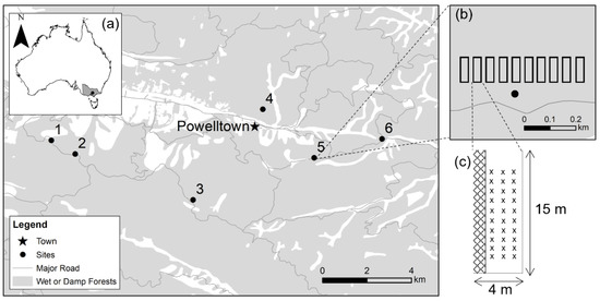
Figure 1.
(a) The location of study sites in the Central Highlands, Victoria, Australia; (b) 10 plots at each site and location of the in-forest weather station (black dot); (c) pattern of gridded ignitions within a plot marked by ‘x’; hashed area shows location where litter samples for laboratory experiments and fuel samples for moisture determination were taken. Sites are as follows: Beenak (1), Fifth Dam (2), Worlleys (3), Bertha (4), Turners (5), and Big Creek (6).
The six study sites were located within a 7 km radius of Powelltown (−37.8650° S, 145.7530° E, and elevation 189 m; Figure 1a and Table A2). Average annual rainfall is 1464 mm for Powelltown, and the average maximum temperature ranges from 11.8 °C in July to 25.4 °C in January [31]. Sites were at least 1 km apart, on a slope of less than 10° and within a > 25 ha patch of wet or damp forest. At each site there were 10 adjacent plots (15 m × 4 m, Figure 1b). One plot was randomly selected for ignition experiments on each ignition date.
2.2. Field Ignition Tests
Experiments were conducted from November to March over two consecutive fire seasons in 2019–20 and 2020–21. For a detailed description of the field experiments, see [28]. All field experiments were conducted under low in-forest wind speeds (<6 km h−1) and between 11 am and 5 pm. In the ignition experiments, a solid cotton cylinder (100% cotton, 3.5 cm length, 1 cm width, and ~0.40 g) was used as a standardised firebrand (obtained from a dental supplier) (Figure 2d). Tests were conducted to compare the combustion dynamics of the cotton cylinder to a natural firebrand, a piece of stringybark (Eucalyptus obliqua), cut to a similar shape and mass as the cotton cylinder (Appendix B). These tests showed the cotton cylinders had a similar heat release rate profile to stringybark (Figure A3). Over the duration of flaming, the mean (±1 SE) maximum heat release rate was 0.18 kJ/s (±0.02) for cotton and 0.16 kJ/s (±0.02) for stringybark (Figure A3).
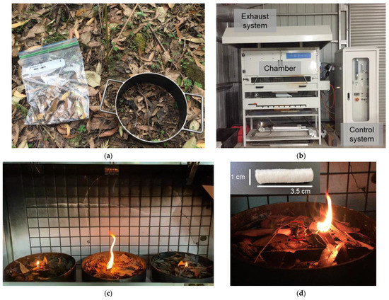
Figure 2.
Photos of litter collection and laboratory experiments: (a) litter collection using 25 cm diameter metal ring; (b) flame propagation apparatus (FPA) showing the exhaust system, chamber and control system; (c) inside FPA chamber, where laboratory ignition experiments occurred; (d) example of laboratory ignition in the early stage of fire initiation, with cotton cylinder shown in red box. Inset (d) shows cotton cylinder firebrand used in laboratory and field experiments. Photos: J. Burton.
Immediately prior to starting the first ignition, fuel moisture was measured for surface litter (recently fallen leaves, twigs and bark less than 6 mm thick lying on the top 1 cm of the litter bed), subsurface litter (leaves, twigs and bark less than 6 mm thick in the lower 1 cm of the litter bed) and near-surface dead fine fuel (dead leaves, bark and twigs less than 6 mm suspended in live vegetation up to a height of 0.5 m (e.g., grasses, shrubs [32])). For each fuel type, samples (mean 157 g wet mass, sd = 81 g and range 92 to 469 g) were collected from five different locations within a 1 m wide strip along the length of the plot and bulked into the same tin (Figure 1c). This tin was sealed to prevent moisture loss, and the samples were then weighed, oven-dried at 105 °C until completely dry and re-weighed to determine the mass of moisture in the sample as a fraction of oven dry mass (hereafter called ‘bulk sample’). A Decagon Weather Station at each site measured screen height (approx. 1.5 m) air temperature, relative humidity, wind speed, wind direction and solar radiation at 10 min intervals (Decagon Devices, Inc., Pullman, WA, USA). Canopy cover was measured in the field from a height of 1.5 m at the centre point of each plot using an iPhone app (PercentCover).
Within each plot, there were 30 ignition points (attempts) arranged in a 3 × 10 grid (Figure 1c). There was a 1 m buffer between plots to allow access while preventing trampling of fuel. Ignitions occurred in a 1 m grid, starting at the downslope end of the plot and working upslope, so that the unburnt ignition points were not trampled (Figure 1c). Prior to each individual ignition, fuel structure was assessed within a 0.5 m radius of each ignition point by visually estimating the cover of surface fine fuel, the cover for near-surface fine fuel and the dead fraction for near-surface fuel. Then, the cotton cylinder was lit using a handheld gas butane lighter. It took approximately 8 s for the cylinder to be fully involved in flame (this was achieved by holding a butane lighter underneath the cotton cylinder). Once flaming, the cotton cylinder was dropped from 30 cm above the top of the fuel-bed layer (litter bed or near-surface) to simulate the fall of a flaming firebrand. Ignition was deemed ‘successful’ (for each attempt) if the surrounding fuel was ignited by the firebrand and burned independently of the ignition source. The ability of the fuel bed to propagate fire was also assessed. Ignition was deemed ‘sustained’ if the fire continued burning for 5 min or burned 0.5 m from the point of ignition. All 30 ignitions within a plot were completed within 1.5 h (mean duration of 64 min and standard deviation of 18 min).
2.3. Litter Collection
We developed a laboratory method to collect litter bed samples, reconstruct them and measure their ignitability in the laboratory. We designed our laboratory method to be (a) achievable during the time field ignitions were being conducted, (b) feasible to conduct given the nature of the vegetation and the location of the study sites and (c) effective in keeping the moisture content and structure of the litter bed similar for reconstruction in the laboratory. Thus, we decided to collect litter into bags rather than taking ‘intact’ or ‘undisturbed’ samples. Whilst intact sampling can be effective at retaining the structure and cover composition of the litter beds [10,33], several factors precluded the use of intact sampling at our study sites. These factors included the dense understorey and slippery vegetation that are difficult to traverse whilst carrying intact samples, rough vehicle tracks that would disturb intact samples and a lack of space within the vehicle to fit large numbers of intact samples.
Five destructive litter samples were taken adjacent to the ignition plot using a 25 cm diameter metal ring with a sharpened edge to cut the litter bed (Figure 2a). The sample size was selected based on previous laboratory studies [14,34,35,36,37] and what was achievable during the time field ignitions were being conducted. Litter was collected as two subsamples, surface and subsurface, to account for variation in moisture content throughout the litter bed and to retain field structure. Surface litter represented recently fallen leaves, twigs and bark lying on the top (~1 cm) of the litter bed with no visible signs of decomposition (as determined by colour and lack of fragmentation) [38]. Subsurface litter included leaves, twigs and bark and other material occurring below the surface material to the bottom of the litter bed, which were often showing signs of decomposition (black colour and leaves not whole) [38]. All material less than 25 mm in diameter was collected. Prior to collection, three evenly distributed litter-depth measurements were taken with a litter-depth gauge [38]. Samples were collected into plastic bags, sealed and stored on ice in foam boxes for transport to the laboratory.
Next to each sample location, a sample (mean 12 g wet mass, standard deviation of 7 g and range 4 to 32 g) of surface and subsurface material was also collected into plastic bags, sealed and stored on ice in foam boxes. These samples were weighed to calculate wet weight, then dried at 105 °C until completely dry and re-weighed, to determine the mass of moisture in the sample as a fraction of oven dry mass. These samples represent the ‘field-measured’ litter moisture content and were used to compare against the ‘lab-measured’ litter moisture content (see Section 2.4).
2.4. Laboratory Ignition Tests
Travel distance from the study sites to the laboratory meant experiments could not be performed on the same day. Samples were stored overnight in a refrigerator to maintain similar moisture content, and tests were conducted within 1.5 days of collection. Before reconstruction, samples were kept in foam boxes in the laboratory for ~30 min to equilibrate to the room ambient conditions. Litter beds were reconstructed into a circular metal tray, which had the same dimensions as the collection ring (25 cm diameter) and was lined with 2.5 cm insulation board to prevent heat loss. Litter was carefully reconstructed by first laying down the subsurface material and then surface material. The litter was gently shaken out of the bag and spread across the area of the metal tray. The litter-bed depth was checked using a ruler at three points spread over the sample before ignition and adjusted if needed to match the field-measured depth. If required, the litter bed was aerated or compressed depending on the change in depth required. Few samples (<15%) required readjusting, and if required this mostly involved aerating the top layer.
A small subsample (3–5 g) from the surface and subsurface litter was taken to calculate laboratory moisture content. This sample contained several elements of each litter component (leaves, twigs and bark). More material was not collected, as this would have disturbed the structure and composition of the sample. These samples were weighed to calculate wet weight, then dried at 105 °C until completely dry and re-weighed, to determine the mass of moisture in the sample as a fraction of oven dry mass. These samples represent the ‘lab-measured’ litter moisture content and were used to compare against the ‘field-measured’ litter moisture content (see Section 2.3).
The laboratory ignition method replicated the field method: a gas lighter was used to ignite the firebrand, which once flaming was dropped from 30 cm above the litter bed into the middle of the circular metal tray. Ignition was deemed ‘successful’ (for each attempt) if the surrounded fuel was ignited by the firebrand (flaming combustion evident beyond firebrand), and ignition was deemed ‘sustained’ if it continued burning for 5 min or burned 0.125 m (radius of sample ring) from the point of ignition (Figure 2d). Ignitions occurred inside the combustion chamber of the flame propagation apparatus (FPA), with up to three samples tested occurring concurrently (Figure 2b,c). The FPA has been designed to test the flammability of fuel beds (Australian Standard AS ISO 9239.1:2003; see Cawson, et al. [39] for detailed description of the apparatus and an example of its use). For our purpose, we used the chamber to place the samples in and the exhaust system to extract gases from the chamber. Fume hood exhaust speed was set to the minimum (<1.8 km h−1).
2.5. Data Analysis
The proportion of successful ignitions and sustained ignitions were calculated for each site on each ignition day using the laboratory and field data. For both data sources, this was calculated as the number of successful or sustained ignitions divided by the total number of attempted ignitions (laboratory, n = 5; field, n = 30). The proportion of successful ignitions and the proportion of sustained ignitions in the field and laboratory tests were compared based on deviation from a 1:1 relationship. The number of observations, for which the laboratory result was an overestimate, underestimate or within 25% of the field result, was calculated for successful and sustained ignitions. This was calculated at two levels: for each site and all sites pooled.
We used Bland–Altman analysis to quantify the level of agreement between the laboratory and the field method [40]. This is a common approach used to compare two methods of measurement, usually a new method with an established or reference method [40]. In this study, the field method represents the reference method for measuring ignition, and the laboratory method represents the new method. We analysed the level of agreement between (a) the moisture content values for each individual litter sample (n = 185) and (b) the ignition results for each site and ignition day (n = 37). The field litter moisture content value was derived from the sample taken adjacent to the litter-bed sample used for the laboratory ignition experiments (see Section 2.3). The differences were checked for normality using histograms, qq plots and the Shapiro–Wilk test. The differences in moisture content were non-normal, so a non-parametric method of calculating the bias and levels of agreement was used [41]. This non-parametric method uses the median difference instead of the mean difference, and the 2.5th and 97.5th percentiles instead of the ±1.96 standard deviation (SD) limits [41]. The results are displayed on Bland–Altman plots that show the mean (or median) difference (bias) between the two methods and the limits of agreement. The plot allows for visual assessment of the agreement between the methods, with a smaller mean bias and range indicating better agreement [40]. The R package BlandAltmanLeh was used for the Bland–Altman analysis [42].
Regression tree modelling was used to identify which factors influence the difference between the laboratory and field results. The response variable was the difference between the observed field and laboratory result (i.e., ignition result (field)—ignition result (laboratory)). Regression tree modelling was chosen as it identifies clear thresholds and is able to handle data limitations (e.g., missing values). We selected predictors that (a) are important to ignitability based on previous studies and/or (b) differed between the laboratory and field setting (e.g., near-surface fuel structure and weather variables). We used Pearson correlation to identify redundant variables (i.e., unrelated to the difference between laboratory and field results and/or highly correlated to another predictor variables) (Figure A1). The final predictors were mean surface litter depth, mean surface litter cover, mean near-surface fuel cover, near-surface fuel moisture content (derived from the bulk sample; Section 2.2), canopy cover and maximum wind speed. Corresponding wind speed data were not available for 7 of 37 observations due to faults in the sites’ weather stations. Two regression trees were created: one for the difference in successful ignitions and one for the difference in sustained ignitions. The regression trees were constructed using the ANOVA method, which splits the data based on a single explanatory variable into progressively smaller groups that maximise homogeneity within the groups while minimising the residual variance [43]. The regression trees were built using the rpart [44] and rpart.plot [45] packages. Variable importance was calculated to indicate the role of each explanatory variable, and R2 was used to measure the fit of the regression tree. All statistical analyses were done in R programming language [46].
3. Results
3.1. Summary of Ignition Results, Fuel Moisture and Weather Conditions over the Study Duration
The total number of plots ignited was 37. Most sites had six plots ignited over the study duration (except Turners, which had 7) (Table A3). The number of successful ignitions ranged from 0 to 30 (proportion: 0 to 1) in the field and 0 to 5 (proportion: 0 to 1) in the laboratory (Table A3). There were no plots in which all point ignitions were sustained in the field or the laboratory. The number of sustained ignitions ranged from 0 to 23 (proportion: 0 to 0.77) in the field and 0 to 2 (proportion: 0 to 0.40) in the laboratory.
The weather conditions during the field experiments varied: maximum temperature ranged from 14 to 38 °C; minimum relative humidity ranged from 20 to 100%; maximum wind speed ranged from 1 to 6 km h−1 (Table A3). Surface litter moisture content ranged from 12% to 257%, and near-surface moisture content ranged from 12% to 99% (Table A3). Litter bed cover ranged from 69% to 100%; near-surface cover ranged from 2% to 56%; litter-bed depth ranged from 19 to 87 mm (Table A3).
3.2. Similarity between the Laboratory and the Field
The surface litter moisture contents were marginally higher in the laboratory compared to the field (bias = −1.46%) (Figure 3a,b). In contrast, the subsurface litter moisture contents were lower in the laboratory compared to the field (bias = 10.28%) (Figure 3c,d). As the moisture content decreased, the difference between the laboratory and field measurements decreased, for both surface and subsurface moisture content (Figure 3b,d).
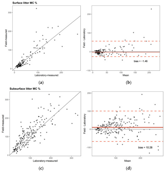
Figure 3.
Comparing moisture content measured in the field and the laboratory: (a) laboratory-measured vs. field-measured surface litter moisture content (MC); (b) Bland–Altman plot for surface litter moisture content; (c) laboratory-measured vs. field-measured subsurface litter moisture content; (d) Bland–Altman plot for subsurface litter moisture content. The solid red line represents the median bias between the laboratory and field results. The dashed red line represents the agreement interval, calculated as the 2.5th and 97.5th percentiles. The solid grey line represents the line of agreement (difference = 0).
The proportion of successful ignitions was generally lower in the laboratory compared to the field (bias = 0.05) (Figure 4a,b). Most of the laboratory results were within 25% of the field results (62% of observations) (Table 1). This was consistent across all sites except Big Creek, where the laboratory result tended to underestimate the field result (Table 1).
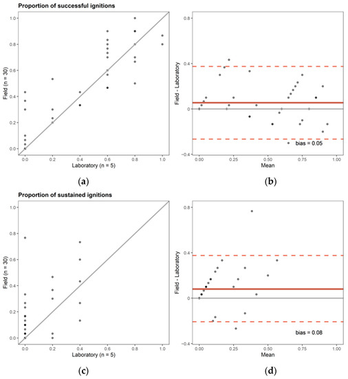
Figure 4.
Comparing ignition measured in the field and the laboratory: (a) laboratory vs. field successful ignition; (b) Bland–Altman plot for successful ignition; (c) laboratory vs. field sustained ignition; (d) Bland–Altman plot for sustained ignition. The solid red line represents the mean difference between the laboratory and field results. The dashed red line represents the agreement interval, calculated as 1.96 × SD. The solid grey line represents the line of agreement (difference = 0).

Table 1.
Similarity between the laboratory and field results by site and all sites pooled. Number of plots belonging to each category, followed by percentage of total in parentheses for all sites.
The proportion of sustained ignitions was lower in the laboratory compared to the field (bias = 0.08) (Figure 4c,d). There were differences between sites for how well the laboratory result matched the field result. Fewer (38%) of the laboratory results were within 25% of the field results (Table 1). The laboratory results tended to underestimate the field results (51%), with the greatest underestimation occurring at the Turners and Fifth Dam sites (Table 1).
3.3. Influence of Fuel and Weather Variables on the Similarity between the Laboratory and the Field
The overall fit (R2) of the regression trees for successful ignitions and sustained ignitions was 0.16 and 0.38, respectively. Near-surface cover and wind speed were the most important variables for predicting the differences in successful ignitions, with the significant thresholds identified (Figure 5, Figure A2). The proportion of successful ignitions was higher in the field compared to the laboratory when there was a substantial cover of near-surface fuel in the field (> 30%) or when the wind speed exceeded 2.4 km h−1 (Figure 5b).
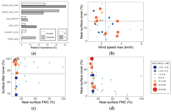
Figure 5.
(a) Relative importance of predictors to the difference between the laboratory and field results for successful and sustained ignitions; hashed lines represent significant predictors (splits); (b) scatterplot of near-surface fuel cover and wind speed for successful ignitions; (c) scatterplot of near-surface fuel moisture and surface litter cover for sustained ignitions; (d) scatterplot of near-surface fuel moisture and near-surface fuel cover for sustained ignitions. Colours and size of points in (b–d) represent size of the difference between field and laboratory results; positive values mean field result was greater than laboratory result (red: underestimation); negative values mean field result was less than laboratory result (blue: overestimation).
Surface litter cover and near-surface fuel moisture content were the most important predictors of the difference in sustained ignitions between the laboratory and the field, with the significant thresholds identified (Figure 5a). The proportion of sustained ignitions was less in the laboratory compared with the field when the near-surface fuel moisture was below 15% and the surface litter cover was above 87% (Figure 5c). When the surface litter cover was lower (<87%), the proportion of sustained ignitions was higher in the laboratory compared with the field. A lower surface litter cover correlated with a higher variability in litter cover (Figure A1). Although a significant threshold in near-surface cover was not identified, the greatest difference (underestimate; difference = 0.77) between the laboratory and field results for sustained ignitions occurred when the near-surface cover was the highest (56%) and the near-surface fuel moisture content was below 15% (Figure 5d, Table A3).
4. Discussion
Collecting accurate data on ignitability is important for developing models to predict spot fire occurrence. We compared how well the results of a laboratory method matched a more complex field method to better understand the scalability of laboratory experiments. We found that the similarity between the results of the laboratory and field methods was greater for successful ignitions than for sustained ignitions. Wind, fuel structure (in the field) and near-surface fuel moisture content influenced how well the results of the laboratory experiment matched the results of the field experiment. We discuss the implications of our work for the design and focus of future laboratory and field experiments.
4.1. Litter Bed Sampling Approach
We designed a method for collecting and reconstructing litter beds that enabled us to measure their ignitability in the laboratory. We designed our method to be achievable and realistic given the experimental context of our study, that is, the nature and location of the study sites and time constraints imposed by the field experiments. There are other methods to measure litter-bed ignitability, such as intact sampling [10,33] or reconstruction using oven-dried or air-dried leaf litter [1,14]. All methods carry their own strengths and limitations, and their suitability depends on the experimental context and study objectives. Although our method is unlikely to suit all experimental contexts, it did have several strengths. For example, our method is one of the first to sample surface and subsurface litter separately, allowing the differences in moisture throughout the litter profile to be retained. Moreover, the transport of litter from the field to the laboratory and subsequent storage did not substantially change the sample moisture content. Thus, we were able to test the ignitability of reconstructed litter beds with realistic (i.e., field) moisture profiles, not those artificially induced by wetting and drying litter samples in the laboratory. Finally, by ensuring that the depth of the reconstructed litter beds matched the field-measured depth, the bulk density of the reconstructed litter beds was comparable to that in the field.
4.2. Similarity between the Laboratory and the Field
The results of the laboratory experiment and the field experiment were similar for the proportion of successful ignitions but less so for sustained ignitions. For successful ignitions, over half the laboratory results were within 25% of the field result (23/37: ~62%), and there were fewer instances of overestimation (8%) compared to underestimation (30%). On the other hand, there was a greater discrepancy between the laboratory and field experiments for the proportion of sustained ignitions, with the laboratory result underestimating the field result half of the time (19/37: ~51%).
The near-surface fuel cover influenced the similarity between the laboratory and field results. For successful ignitions, increased cover (above 30%) of near-surface fuel was associated with greater underestimation. Likewise, for sustained ignitions, greater cover of near-surface fuel, coupled with dry (<15% fuel moisture content) dead near-surface fuel, was associated with greater underestimation. At higher values of near-surface cover, there is a greater potential for firebrand ignitions to occur in the near-surface fuel rather than the surface litter. When the dead component of near-surface fuel is available to burn but that of the surface litter is not, this leads to more ignitions occurring in the field than in the laboratory. Sustained ignitions in near-surface fuel have also been observed by Buckley [47] in regrowth eucalypt forest, where fires were able to ignite and sustain in wiregrass above the litter bed when the moisture content of surface litter was greater than 20%.
More sustained ignitions occurred in the laboratory than the field when the surface litter cover was lower and more variable. At some sites (e.g., Big Creek), there were patches of bare ground and litter mixed with soil, which may have been due to faunal disturbance (e.g., lyrebirds) [48]. In these instances, a greater proportion of firebrands landed on bare soil and, thus, were unable to sustain (spread to 0.5 m). These discontinuities in the litter bed were not captured in the laboratory, as the litter was sampled from the areas where it was present, and a smaller spread threshold was used (0.125 m). Similarly, Lyon, et al. [49] found that fuel discontinuities in the field contributed to differences between observed (field) and predicted (from laboratory-derived models) fire behaviour (flame length and rate of spread).
Differences in weather conditions between the two experimental settings also influenced the similarity between the laboratory and field results. Previous studies have found that the presence of wind in the field but not in the laboratory causes a disparity between the laboratory and field outcomes [25,49]. In our study, maximum field wind speed explained some of the discrepancy between the laboratory and field results for the proportion of successful ignitions. When the wind speed was above 2.4 km h−1 in the field, there were more instances of underestimation, that is, there were fewer ignitions measured in the laboratory than the field. Higher wind speeds in the field (compared to zero-wind conditions in the laboratory) may support more successful ignitions, as wind can increase the heat transfer to unburnt fuel and increase the probability of ignition [14]. However, it is important to note that the field experiments occurred under a narrow range of wind conditions (1 to 6 km h−1). At higher wind speeds, wind may hinder ignition by decreasing the temperature of the firebrand and fuel bed [15]. For example, previous laboratory studies have found ignition probability increases with increasing wind speed and then reaches a threshold where wind inhibits ignition [10,16]. Thus, the influence of wind on the similarity between the laboratory and field results is likely to change with increasing wind speed.
There may be other factors influencing the dissimilarity between the laboratory and field results. The difference in sample size (5 ignition attempts in the laboratory vs. 30 ignition attempts in the field) means there is greater uncertainty associated with the laboratory estimates. Whilst it would have been valuable to collect more samples for the laboratory tests, the number of samples collected represents the maximum that could be feasibly achieved during the time the field experiments were being conducted. The strength of the regression tree to explain the difference between the laboratory and field results was not strong, particularly for the proportion of successful ignitions (R2 = 0.16 vs. 0.38 for sustained ignitions). That said, the similarity between the laboratory and field results was higher for successful ignitions than for sustained ignitions. Nevertheless, there may be additional (unmeasured) factors such as where the firebrand lands, the microtopography and shading from understorey fuel in the field. For example, litter components (e.g., leaves, bark or twigs) differ in their ignition potential [50], so where the firebrand lands may influence ignition success.
4.3. Implications and Next Steps
Most laboratory studies tend to focus only on litter beds, as they are assumed to be the main fuel layer where firebrands land and fires start to spread [1,10,33]. This approach may give similar results as field experiments in forests where there is sparse near-surface fuel and where the litter bed is the dominant receiving layer for firebrands. However, it may be less suitable for forests where there is dense cover of near-surface vegetation. By only studying the litter bed, the effect and interaction with other fuel strata (e.g., near-surface fuels) is not captured, which may lead to inaccurate estimations of ignitability, as we have shown here. Few laboratory studies incorporate both litter and near-surface fuel into their experimental design (however, see Cawson, Pickering, Penman and Filkov [39] for an example). Similarly, few laboratory studies incorporate variability in surface litter cover. Both of these attributes in addition to wind should be an important focus of laboratory and field experiments going forward.
The comparison between the laboratory and field results creates interesting avenues for future research. For instance, the greatest difference between the laboratory and field results occurred when the near-surface cover was high (> 30%) and available to burn but when the surface litter was difficult to ignite (16% to 22% moisture content). This raises interesting questions such as: Would fire propagate entirely in the near-surface fuel? How much near-surface fuel is enough for fire to only spread in it? Would the heat from the burning of near-surface fuel dry out the litter bed enough to facilitate the burning of surface litter? Other important considerations are the firebrand type and size and the accumulation of firebrands. We tested the ignition probability from a single flaming firebrand, but ignition likelihood would vary with the number and type of firebrands [11,12,51,52].
Future experimental studies in the laboratory and the field may be able to answer these questions. In the field, the methodology could be expanded to collect data on where the ignition takes place (e.g., litter bed or near-surface fuel) and whether it transitions from one fuel strata to the other. In the laboratory, intermediate-scale (5–10 m) experimental facilities need to be developed that allow for the reconstruction of both litter and near-surface fuel.
5. Conclusions
Research to better understand the conditions when litter beds will ignite from firebrands is critical for developing models to predict spot fire occurrence. We found that a laboratory method provided similar results to a field method for measuring ignition success. However, due to factors not currently integrated into the standard laboratory setting (e.g., near-surface fuel), small-scale laboratory experiments may not provide suitable surrogates for measuring sustained ignition across all forest types. Small-scale laboratory experiments may be more applicable to forests where near-surface cover is low and where firebrands fall predominately on the surface litter bed. Future studies using concurrent field and larger-scale laboratory approaches are needed to examine the role of near-surface fuel in the ignition and propagation processes. Such experiments would provide valuable data for developing models to predict ignition probability from firebrands in forests where there is greater cover of near-surface fuel, such as wet eucalypt forests. Importantly, our study highlights the value of performing laboratory and field experiments simultaneously for a greater understanding of fire behaviour.
Author Contributions
Conceptualisation, J.E.B., J.G.C., A.I.F. and T.D.P.; methodology, J.E.B., J.G.C., A.I.F. and T.D.P.; data collection, J.E.B., B.J.P., J.G.C., A.I.F. and T.D.P.; formal analysis, J.E.B.; writing—original draft preparation, J.E.B.; writing—review and editing, J.E.B., B.J.P., J.G.C., A.I.F. and T.D.P.; supervision, J.G.C., A.I.F. and T.D.P.; project administration, J.E.B., B.J.P., J.G.C., A.I.F. and T.D.P.; funding acquisition, J.G.C. and T.D.P. All authors have read and agreed to the published version of the manuscript.
Funding
This research was funded by the Victorian Government’s Department of Environment, Land, Water and Planning (DELWP).
Institutional Review Board Statement
Not applicable.
Informed Consent Statement
Not applicable.
Data Availability Statement
The data that support this study will be shared upon reasonable request to the corresponding author.
Acknowledgments
The authors thank the industry leads for this project, Andrew Ackland (Country Fire Authority) and Musa Kilinc (Country Fire Authority), for their role in the development and coordination of the broader project. Thanks to the Department of Environment, Land, Water and Planning (DELWP) and Parks Victoria staff for providing time and resources for the field experiments. Thanks to Wendy Burton and Joseph Hall for their assistance with sample storage and transport.
Conflicts of Interest
The authors declare no conflict of interest.
Appendix A
Table A1.
Summary of past studies that investigate ignitability in the laboratory and field.
Table A1.
Summary of past studies that investigate ignitability in the laboratory and field.
| Field or Laboratory | Author; Location | Purpose of Study | Ignition Source | Definition of Successful Ignition |
|---|---|---|---|---|
| Field | [28]; eucalypt forest in Victoria | Evaluate different in-forest and landscape variables as predictors of ignitability | Cotton cylinder and sawdust–wax firelighter | (1) Fuel ignited and burnt independently of ignition source (2) Flaming sustained 0.5 m from the point of ignition or 5 min |
| Field | [23]; eucalypt forest in Victoria | Identify drivers of ignitability during a prescribed burn | Drip torch lit in strips to create backing fire | Flaming self-sustains beyond the point of ignition |
| Field | [53]; heathland, UK | Quantify the variation in fire sustainability | Drip torch (3 × spots followed by 2 m strip) | Fire spreads 2 m in less than 5 min |
| Field | [22]; grassland, Greece | Develop a model to predict ignition probability | Drip torch (10 m strips); five ignition trials per test | Flaming sustained for >1 min in 5 consecutive ignition trials |
| Field | [54]; Australian alps | Quantify flammability of alpine vegetation | Kerosene fire lighting blocks | Flaming sustained > 5 s |
| Field | [55]; Tasmanian grasslands | Identify thresholds for fire spread in grasslands | Drip torch (2 m strip) | Fire spread 2 m and visual descriptors |
| Field | [21]; gorse stands, New Zealand | Identify thresholds for ignition and fire spread in gorse stands | Alternated between use of a drip torch and a standard cigarette lighter, fuel ignited at height of 0.5 m | Fire spread to top of gorse clump and burned clump completely |
| Laboratory | [10]; dry eucalypt litter in laboratory | Measure the probability of ignition | Flaming firebrands were 50 mm bamboo satay sticks; glowing firebrands were 50 × 15 mm E. globulus bark pieces | Flaming sustained for 60 s |
| Laboratory | [12]; pine needle litter bed | Quantify the effect of firebrand size and wind speed on litter ignition | Pine bark of various sizes; ignition attempted first with single firebrand, then up to 10 firebrands together | Flaming—visible flaming of needles within fuel bed Smouldering—smouldering of fuel bed |
| Laboratory | [51]; pine needle litter bed | Quantify the effect of firebrand size and type, fuel bulk density and wind speed on time to flaming ignition | Pine bark and twigs of various sizes; fuel bed was exposed to a single firebrand | Flaming—visible flaming of needles within fuel bed |
| Laboratory | [1]; litter beds of European species | Quantify flammability of different litter beds | Cubes of Pinus sylvestris wood ignited using an electric radiator | Time to ignition |
| Laboratory | [14]; litter beds of shrub fuel | Identify factors influencing ignition in the litter bed of shrublands | Cotton balls soaked in 1 mL methylated spirits (to emulate aerial incendiary) | Fire spread 12.5 cm to edge of fuel tray from ignition point |
Table A2.
Site attributes. Means (with standard deviation in parentheses) reported for canopy cover and litter-bed depth.
Table A2.
Site attributes. Means (with standard deviation in parentheses) reported for canopy cover and litter-bed depth.
| Site No. | Site | Lat, Long | Canopy Cover (%) | Litter-Bed Depth (mm) | Dominant Overstorey Species |
|---|---|---|---|---|---|
| 1 | Beenak | −37.8712, 145.6708 | 71 (4) | 36 (11) | Eucalyptus obliqua L’Hér, E. regnans F.Muell. |
| 2 | Fifth Dam | −37.8766, 145.6805 | 65 (2) | 42 (21) | E. obliqua |
| 3 | Worlleys | −37.8950, 145.7281 | 67 (4) | 30 (12) | E. regnans |
| 4 | Bertha | −37.8586, 145.7562 | 66 (4) | 62 (4) | E. cypellocarpa L.A.S.Johnson, E. sieberi L.A.S.Johnson, E. obliqua |
| 5 | Turners | −37.8781, 145.7770 | 62 (8) | 33 (17) | E. regnans |
| 6 | Big Creek | −37.8705, 145.8044 | 66 (6) | 27 (9) | E. regnans |
Table A3.
Summary of ignition results, fuel moisture content (FMC), fuel structure data and weather recorded during the ignition experiments.
Table A3.
Summary of ignition results, fuel moisture content (FMC), fuel structure data and weather recorded during the ignition experiments.
| Site | Date | Successful Ignitions | Sustained Ignitions | Surface Litter FMC a | Near-Surface FMC a | Mean Litter Bed Cover (%) | Mean Near-Surface Cover (%) | Mean Litter Bed Depth (mm) | Max Wind Speed (km h−1) b | Min RH (%) b | Max Temp (°C) b | ||
|---|---|---|---|---|---|---|---|---|---|---|---|---|---|
| Lab | Field | Lab | Field | ||||||||||
| Beenak | 17 December 2019 | 0.60 | 0.80 | 0 | 0.17 | 21.7 | 20.1 | 95 | 11 | 38 | 2.4 | 40.1 | 26.1 |
| 30 January 2020 | 0.80 | 1 | 0.40 | 0.73 | 16.6 | 13.9 | 99 | 43 | 27 | 2.1 | 21.1 | 35.2 | |
| 18 November 2020 | 0.80 | 0.70 | 0.20 | 0.47 | 17.2 | 17.4 | 88 | 13 | 25 | 1.7 | 24.7 | 25.2 | |
| 14 December 2020 | 1 | 0.80 | 0.40 | 0.43 | 20.2 | 17.1 | 99 | 26 | 51 | 1.4 | 31.9 | 30.6 | |
| 16 February 2021 | 0.20 | 0.30 | 0 | 0 | 26.8 | 19.9 | 95 | 16 | 41 | 0.9 | 65.1 | 26.5 | |
| 30 March 2021 | 0 | 0 | 0 | 0 | 99.4 | 23.9 | 96 | 9 | 28 | 2.2 | 72.6 | 23.5 | |
| Bertha | 17 December 2019 | 0 | 0.43 | 0 | 0.10 | 25.1 | 21.7 | 100 | 30 | 39 | 3.6 | 36.3 | 26.3 |
| 18 March 2020 | 0.40 | 0.33 | 0 | 0 | 20.8 | 17.1 | 100 | 9 | 32 | 2.3 | 24.1 | 34.2 | |
| 11 December 2020 | 0.20 | 0.23 | 0 | 0 | 35.6 | 31.1 | 100 | 17 | 32 | 4.9 | 45.2 | 20.9 | |
| 15 December 2020 | 0.80 | 0.90 | 0 | 0.27 | 17.7 | 14.7 | 95 | 19 | 38 | 2.7 | 29.9 | 32.9 | |
| 16 February 2021 | 0.40 | 0.43 | 0 | 0.07 | 23.8 | 20.8 | 99 | 3 | 56 | 2.4 | 61.8 | 24.2 | |
| 30 March 2021 | 0 | 0 | 0 | 0 | 190.2 | 75.5 | 97 | 2 | 55 | 2.5 | 95.0 | 14.0 | |
| Big Creek | 19 December 2019 | 0 | 0.37 | 0 | 0.03 | 28.5 | 21.9 | 78 | 36 | 29 | 1.5 | 42.4 | 29.7 |
| 18 March 2020 | 0 | 0.06 | 0 | 0 | 73.0 | 33.5 | 81 | 9 | 19 | NA | 33.5 | 31.5 | |
| 11 December 2020 | 0 | 0.30 | 0 | 0.03 | 67.7 | 20.3 | 93 | 30 | 24 | 1.5 | 82.2 | 20.1 | |
| 15 December 2020 | 0.60 | 0.60 | 0.40 | 0.13 | 16.9 | 15.9 | 84 | 31 | 25 | 2.1 | 33.7 | 31.2 | |
| 16 February 2021 | 0 | 0.10 | 0 | 0 | 53.6 | 31.0 | 85 | 7 | 23 | NA | 73.0 | 24.1 | |
| 31 March 2021 | 0 | 0 | 0 | 0 | 257.3 | 56.2 | 79 | 3 | 21 | NA | 100.0 | 14.1 | |
| Fifth Dam | 17 December 2019 | 0.60 | 0.47 | 0 | 0.03 | 18.6 | 18.5 | 91 | 26 | 38 | 3.1 | 35.9 | 28.6 |
| 30 January 2020 | 0.60 | 0.90 | 0.20 | 0.30 | 12.8 | 12.7 | 97 | 13 | 35 | 3.6 | 20.6 | 33.1 | |
| 18 November 2020 | 0.60 | 0.70 | 0.20 | 0.37 | 17.7 | 14.7 | 74 | 14 | 26 | 2.6 | 29.7 | 26.1 | |
| 14 December 2020 | 0.80 | 0.90 | 0 | 0.77 | 18.1 | 14.0 | 99 | 56 | 40 | 2.1 | 32.8 | 31.2 | |
| 17 February 2021 | 0.80 | 0.67 | 0 | 0.23 | 18.2 | 18.3 | 100 | 14 | 87 | 2.1 | 51.4 | 27.4 | |
| 30 March 2021 | 0 | 0.03 | 0 | 0 | 110.8 | 54.3 | 93 | 7 | 24 | 1.5 | 79.5 | 14.6 | |
| Turners | 19 December 2019 | 0.60 | 0.83 | 0 | 0.33 | 14.3 | 11.7 | 97 | 49 | 27 | 1.9 | 34.8 | 32.0 |
| 30 January 2020 | 0.60 | 0.77 | 0.40 | 0.27 | 16.1 | 12.6 | 99 | 31 | 27 | 1.9 | 26.6 | 37.6 | |
| 18 March 2020 | 0.60 | 0.73 | 0 | 0.10 | 24.1 | 18.5 | 99 | 29 | 30 | 1.3 | 46.5 | 31.0 | |
| 11 December 2020 | 0.40 | 0.33 | 0 | 0.00 | 17.6 | 15.9 | 99 | 17 | 35 | 5.9 | 47.6 | 24.8 | |
| 15 December 2020 | 1 | 0.87 | 0.40 | 0.60 | 12.4 | 14.0 | 98 | 35 | 31 | 2.8 | 27.6 | 36.4 | |
| 17 February 2021 | 0.60 | 0.57 | 0 | 0.10 | 27.8 | 16.4 | 100 | 22 | 39 | 2.7 | 37.0 | 38.4 | |
| 31 March 2021 | 0 | 0 | 0 | 0 | 102.5 | 47.2 | 97 | 24 | 37 | 1.6 | 85.3 | 19.1 | |
| Worlleys | 19 December 2019 | 0.20 | 0.53 | 0.20 | 0 | 20.1 | 15.9 | 69 | 7 | 30 | 3.6 | 32.6 | 25.1 |
| 30 January 2020 | 0.60 | 0.47 | 0 | 0.13 | 13.3 | 14.6 | 97 | 46 | 34 | 1.2 | 20.7 | 32.4 | |
| 18 November 2020 | 0.80 | 0.50 | 0.20 | 0.03 | 14.4 | 16.3 | 76 | 5 | 30 | NA | 30.0 | 23.1 | |
| 14 December 2020 | 0.80 | 0.80 | 0 | 0.17 | 18.9 | 17.6 | 96 | 27 | 32 | NA | 38.6 | 29.3 | |
| 17 February 2021 | 0.20 | 0.20 | 0 | 0 | 40.3 | 32.4 | 93 | 26 | 45 | NA | 70.5 | 23.3 | |
| 31 March 2021 | 0 | 0 | 0 | 0 | 141.3 | 99.3 | 93 | 30 | 37 | NA | 98.2 | 16.9 | |
a Fuel moisture content (FMC) measured in the field using bulk sample (see Section 2.2). b Weather variables at the time field ignitions occurred, extracted from in-situ weather station at each site.

Figure A1.
Correlogram showing the strength of Pearman’s correlations between the difference (i.e., ignition result (field)—ignition result (laboratory)) and potential predictor variables. Positive correlations are displayed in blue and negative correlations in red. Colour intensity is proportional to the correlation coefficient. Variables with * were used in final analysis. Variables: DIFF_SUCCESS = difference in proportion of successful ignitions, DIFF_SUSTAINED = difference in proportion of sustained ignitions, SUR_DEPTH = litter-bed depth, SUR_COV = litter-bed cover, SUR_COV_VAR = coefficient of variation in litter-bed cover, NEAR_SUR_COV = near-surface cover, NEAR_SUR_COV_VAR = coefficient of variation in near-surface cover, NEAR_SUR_DEAD = near-surface dead fraction, CANOPY_COV = canopy cover, SUR_FMC = surface litter moisture content (bulk sample), NEAR_SUR_FMC = near-surface dead fuel moisture content (bulk sample), WIND_MEAN = average wind speed, WIND_MAX = maximum wind speed, RH_MIN = minimum relative humidity, TEMP_MAX = maximum temperature, and VPD_MAX = maximum vapour pressure deficit.

Figure A2.
Regression trees for the difference between the field and laboratory result: (a) proportion of successful ignitions (R2 = 0.16); (b) proportion of sustained ignitions (R2 = 0.38).
Appendix B. Comparing Combustion Dynamics of Cotton Cylinder to Stringybark Firebrand
The solid cotton cylinders were obtained from a dental supplier. Stringybark samples (Eucalyptus obliqua) were collected from eucalypt plantations adjacent to the Creswick Campus, Victoria, Australia. The plantations are approximately 30 years old and are unburnt, meaning the bark is free of char. Bark (~0.5 cm depth) was peeled off 2–3 trees and taken to the laboratory. The bark firebrands were cut to match the shape and mass (~0.40 g) of the cotton cylinder (Table A4). All firebrands were left to air-dry on a bench indoors to ambient conditions for 24 h before the experiments.
Five tests were conducted per firebrand. The ignition experiments were conducted on a bench top. The firebrand was placed in a holder, which sat on a set of scales (0.01 accuracy). The firebrand was ignited using a handheld butane lighter (applied for approximately 8 s). The mass loss was recorded continuously. The start of flaming (independent from the ignition source) and end of flaming were recorded. They were used to calculate the flaming duration. The heat release rate (kJ/s) was calculated by multiplying the mass loss rate by the heat of combustion for each time step. The heat of combustion was determined using an oxygen bomb calorimeter. The heat of combustion was 16.3 MJ kg−1 for the cotton cylinder and 19.2 MJ kg−1 for stringybark. Generalised additive models (GAMs) were used to derive the mean heat release rate curves for each firebrand as a function of time (Figure A3).
Table A4.
Specifications of firebrands.
Table A4.
Specifications of firebrands.
| Firebrand | Shape and Dimensions | Weight (g) | Area (cm2) | Volume (cm3) |
|---|---|---|---|---|
| Cotton Cylinder | Cylinder 3.5 cm long × 1 cm wide | 0.43 (± 0.05) | 12.6 | 2.75 |
| Stringybark (Eucalyptus obliqua) | Rectangle 3.5 cm long × 1 cm wide × 0.4 cm deep | 0.41 (± 0.03) | 10.6 | 1.4 |

Figure A3.
Mean heat release rate of stringybark (black) and cotton cylinder (grey). Dashed lines represent the mean flaming duration (stringybark = 40 s; cotton = 57 s). Error bars represent ± 1 standard error.
References
- Ganteaume, A.; Lampin-Maillet, C.; Guijarro, M.; Hernando, C.; Jappiot, M.; Fonturbel, T.; Perez-Gorostiaga, P.; Vega, J.A. Spot fires: Fuel bed flammability and capability of firebrands to ignite fuel beds. Int. J. Wildland Fire 2009, 18, 951–969. [Google Scholar] [CrossRef]
- Sullivan, A.L.; McCaw, L.; Cruz, M.G.; Matthews, S.; Ellis, P.F. Fuel, fire weather and fire behaviour in australian ecosystems. In Flammable Australia: Fire Regimes, Biodiversity and Ecosystems in a Changing World; Bradstock, R., Gill, A.M., Williams, R.J., Eds.; CSIRO Publishing: Melbourne, VIC, Australia, 2012. [Google Scholar]
- Filkov, A.I.; Duff, T.J.; Penman, T.D. Frequency of dynamic fire behaviours in australian forest environments. Fire 2019, 3, 1. [Google Scholar] [CrossRef]
- Wang, H.-H. Analysis on downwind distribution of firebrands sourced from a wildland fire. Fire Technol. 2009, 47, 321–340. [Google Scholar] [CrossRef]
- Koo, E.; Pagni, P.J.; Weise, D.R.; Woycheese, J.P. Firebrands and spotting ignition in large-scale fires. Int. J. Wildland Fire 2010, 19, 818–843. [Google Scholar] [CrossRef]
- Varner, J.M.; Kane, J.M.; Kreye, J.K.; Engber, E. The flammability of forest and woodland litter: A synthesis. Curr. For. Rep. 2015, 1, 91–99. [Google Scholar] [CrossRef]
- Ganteaume, A.; Guijarro, M.; Jappiot, M.; Hernando, C.; Lampin-Maillet, C.; Pérez-Gorostiaga, P.; Vega, J.A. Laboratory characterization of firebrands involved in spot fires. Ann. For. Sci. 2011, 68, 531–541. [Google Scholar] [CrossRef]
- Fateev, V.; Agafontsev, M.; Volkov, S.; Filkov, A. Determination of smoldering time and thermal characteristics of firebrands under laboratory conditions. Fire Saf. J. 2017, 91, 791–799. [Google Scholar] [CrossRef]
- Manzello, S.L.; Cleary, T.G.; Shields, J.R.; Yang, J.C. Ignition of mulch and grasses by firebrands in wildland—Urban interface fires. Int. J. Wildland Fire 2006, 15, 427–431. [Google Scholar] [CrossRef]
- Ellis, P.F.M. The likelihood of ignition of dry-eucalypt forest litter by firebrands. Int. J. Wildland Fire 2015, 24, 225–235. [Google Scholar] [CrossRef]
- Hakes, R.S.P.; Salehizadeh, H.; Weston-Dawkes, M.J.; Gollner, M.J. Thermal characterization of firebrand piles. Fire Saf. J. 2019, 104, 34–42. [Google Scholar] [CrossRef]
- Kasymov, D.P.; Filkov, A.I.; Baydarov, D.A.; Sharypov, O.V. Interaction of Smoldering Branches and Pine Bark Firebrands with Fuel Bed at Different Ambient Conditions; SPIE—The International Society for Optical Engineering: Bellingham, WA, USA, 2016. [Google Scholar]
- Fernandez-Pello, A.C. Wildland fire spot ignition by sparks and firebrands. Fire Saf. J. 2017, 91, 2–10. [Google Scholar] [CrossRef]
- Plucinski, M.P.; Anderson, W.R. Laboratory determination of factors influencing successful point ignition in the litter layer of shrubland vegetation. Int. J. Wildland Fire 2008, 17, 628–637. [Google Scholar] [CrossRef]
- Yang, G.; Ning, J.; Shu, L.; Zhang, J.; Yu, H.; Di, X. Spotting ignition of larch (Larix gmelinii) fuel bed by different firebrands. J. For. Res. 2021, 33, 171–181. [Google Scholar] [CrossRef]
- Sun, P.; Zhang, Y.; Sun, L.; Hu, H.; Guo, F.; Wang, G.; Zhang, H. Influence of fuel moisture content, packing ratio and wind velocity on the ignition probability of fuel beds composed of mongolian oak leaves via cigarette butts. Forests 2018, 9, 507. [Google Scholar] [CrossRef]
- Bryam, G.M. Combustion of forest fuels. In Forest Fire: Control and Use; McGraw-Hill Book Company: New York, NY, USA, 1959; pp. 61–89. [Google Scholar]
- Matthews, S. Dead fuel moisture research: 1991–2012. Int. J. Wildland Fire 2014, 23, 78–92. [Google Scholar] [CrossRef]
- Pickering, B.J.; Duff, T.J.; Baillie, C.; Cawson, J.G. Darker, cooler, wetter: Forest understories influence surface fuel moisture. Agric. For. Meteorol. 2021, 300, 108311. [Google Scholar] [CrossRef]
- Burton, J.E.; Cawson, J.G.; Filkov, A.I.; Penman, T.D. Leaf traits predict global patterns in the structure and flammability of forest litter beds. J. Ecol. 2021, 109, 1344–1355. [Google Scholar] [CrossRef]
- Anderson, S.A.J.; Anderson, W.R. Ignition and fire spread thresholds in gorse (Ulex europaeus). Int. J. Wildland Fire 2010, 19, 589–598. [Google Scholar] [CrossRef]
- Dimitrakopoulos, A.P.; Mitsopoulos, I.D.; Gatoulas, K. Assessing ignition probability and moisture of extinction in a mediterranean grass fuel. Int. J. Wildland Fire 2010, 19, 29–34. [Google Scholar] [CrossRef]
- Cawson, J.G.; Duff, T.J. Forest fuel bed ignitability under marginal fire weather conditions in Eucalyptus forests. Int. J. Wildland Fire 2019, 28, 198–204. [Google Scholar] [CrossRef]
- Tanskanen, H.; Venäläinen, A.; Puttonen, P.; Granström, A. Impact of stand structure on surface fire ignition potential in Picea abies and Pinus sylvestris forests in southern finland. Can. J. For. Res. 2005, 35, 410–420. [Google Scholar] [CrossRef]
- Schiks, T.J.; Wotton, B.M. Assessing the probability of sustained flaming in masticated fuel beds. Can. J. For. Res. 2015, 45, 68–77. [Google Scholar] [CrossRef]
- Van Wagner, C. Two Solitudes in Forest Fire Research; Canadian Forestry Service: Gainesville, FL, USA, 1971.
- Fernandes, P.M.; Cruz, M.G. Plant flammability experiments offer limited insight into vegetation–fire dynamics interactions. New Phytol. 2012, 194, 606–609. [Google Scholar] [CrossRef]
- Cawson, J.G.; Pickering, B.J.; Filkov, A.I.; Burton, J.E.; Kilinc, M.; Penman, T.D. Predicting ignitability from firebrands in mature wet eucalypt forests. For. Ecol. Manag. 2022, 519, 120315. [Google Scholar] [CrossRef]
- Finlayson, B.L.; McMahon, T.A.; Peel, M.C. Updated world map of the köppen-geiger climate classification. Hydrol. Earth Syst. Sci. 2007, 11, 1633–1644. [Google Scholar]
- Ashton, D.H.; Attiwill, P.M. Tall open-forests. In Australian Vegetation, 2nd ed.; Groves, R.H., Ed.; Cambridge University Press: Oakleigh, VIC, Australia, 1994; pp. 157–196. [Google Scholar]
- Bureau of Meteorology. Climate Statistics for Australian Locations. Available online: http://www.bom.gov.au/climate/averages/tables/cw_086094.Shtml (accessed on 27 April 2022).
- Hines, F.; Tolhurst, K.G.; Wilson, A.A.G.; McCarthy, G.J. Overall Fuel Hazard Assessment Guide; Victorian Government Department of Sustainability and Environment: Melbourne, VIC, Australia, 2010.
- Ganteaume, A.; Jappiot, M.; Curt, T.; Lampin, C.; Borgniet, L. Flammability of litter sampled according to two different methods: Comparison of results in laboratory experiments. Int. J. Wildland Fire 2014, 23, 1061–1075. [Google Scholar] [CrossRef]
- Bianchi, L.O.; Defossé, G.E. Ignition probability of fine dead surface fuels of native patagonian forests of argentina. For. Syst. 2014, 23, 129–138. [Google Scholar] [CrossRef]
- Blauw, L.G.; Wensink, N.; Bakker, L.; van Logtestijn, R.S.; Aerts, R.; Soudzilovskaia, N.A.; Cornelissen, J.H. Fuel moisture content enhances nonadditive effects of plant mixtures on flammability and fire behavior. Ecol. Evol. 2015, 5, 3830–3841. [Google Scholar] [CrossRef]
- Cornwell, W.K.; Elvira, A.; van Kempen, L.; van Logtestijn, R.S.; Aptroot, A.; Cornelissen, J.H. Flammability across the gymnosperm phylogeny: The importance of litter particle size. New Phytol. 2015, 206, 672–681. [Google Scholar] [CrossRef]
- Grootemaat, S.; Wright, I.J.; van Bodegom, P.M.; Cornelissen, J.H.C. Scaling up flammability from individual leaves to fuel beds. Oikos 2017, 126, 1428–1438. [Google Scholar] [CrossRef]
- McCarthy, G.J. Surface Fine Fuel Hazard Rating—Forest Fuels; Forest Science Centre, Department of Sustainability and Environment: Orbost, VIC, Australia, 2004. [Google Scholar]
- Cawson, J.G.; Pickering, B.; Penman, T.D.; Filkov, A. Quantifying the effect of mastication on flaming and smouldering durations in eucalypt forests and woodlands under laboratory conditions. Int. J. Wildland Fire 2021, 30, 611–624. [Google Scholar] [CrossRef]
- Bland, J.; Altman, D. Measuring agreement in method comparison studies. Stat. Methods Med. Res. 1999, 8, 135–160. [Google Scholar] [CrossRef]
- Twomey, P.J. How to use difference plots in quantitative method comparison studies. Ann. Clin. Biochem. 2006, 43, 124–129. [Google Scholar] [CrossRef]
- Lehnert, B. Blandaltmanleh: Plots (Slightly Extended) Bland-Altman Plots, 0.3.1. R Package Version 0.3.1. 2015. Available online: https://cran.r-project.org/web/packages/BlandAltmanLeh/index.html (accessed on 1 September 2022).
- De’ath, G.; Fabricius, K.E. Classification and regression trees: A powerful yet simple technique for ecological data analysis. Ecology 2000, 81, 3178–3192. [Google Scholar] [CrossRef]
- Therneau, T.; Atkinson, B.; TRipley, B. Package ‘rpart’ Recursive Partitioning and Regression Trees, R Package Version 4.1.16. 2019. Available online: https://cran.r-project.org/web/packages/rpart/rpart.pdf (accessed on 21 May 2021).
- Milborrow, S. Package ‘rpart.Plot’ Plot ‘part’ Models: An Enhanced Version of ‘plot.Rpart’, R Package Version 3.1.1. 2020. Available online: https://cran.r-project.org/web/packages/rpart.plot/rpart.plot.pdf (accessed on 21 May 2021).
- R Development Core Team. R: A Language and Environment for Statistical Computing, 4.2.1; R Foundation for Statistical Computing: Vienna, Austria, 2022. [Google Scholar]
- Buckley, A.J. Fuel Reducing Regrowth Forests with a Wiregrass Fuel Type: Fire Behaviour Guide and Prescriptions; Fire Management Branch, Department of Conservation and Natural Resources: East Melbourne, VIC, Australia, 1993; pp. 1–34.
- Nugent, D.T.; Leonard, S.W.J.; Clarke, M.F. Interactions between the superb lyrebird (Menura novaehollandiae) and fire in south-eastern Australia. Wildl. Res. 2014, 41, 203–211. [Google Scholar] [CrossRef]
- Lyon, Z.D.; Morgan, P.; Stevens-Rumann, C.S.; Sparks, A.M.; Keefe, R.F.; Smith, A.M.S. Fire behaviour in masticated forest fuels: Lab and prescribed fire experiments. Int. J. Wildland Fire 2018, 27, 280–292. [Google Scholar] [CrossRef]
- Grootemaat, S.; Wright, I.J.; van Bodegom, P.M.; Cornelissen, J.H.C.; Shaw, V. Bark traits, decomposition and flammability of australian forest trees. Aust. J. Bot. 2017, 65, 327–338. [Google Scholar] [CrossRef]
- Matvienko, O.V.; Kasymov, D.P.; Filkov, A.I.; Daneyko, O.I.; Gorbatov, D.A. Simulation of fuel bed ignition by wildland firebrands. Int. J. Wildland Fire 2018, 27, 550–561. [Google Scholar] [CrossRef]
- Suzuki, S.; Manzello, S.L.; Kagiya, K.; Suzuki, J.; Hayashi, Y. Ignition of mulch beds exposed to continuous wind-driven firebrand showers. Fire Technol. 2015, 51, 905–922. [Google Scholar] [CrossRef]
- Davies, G.M.; Legg, C.J. Fuel moisture thresholds in the flammability of calluna vulgaris. Fire Technol. 2011, 47, 421–436. [Google Scholar] [CrossRef]
- Fraser, I.P.; Williams, R.J.; Murphy, B.P.; Camac, J.S.; Vesk, P.A. Fuels and landscape flammability in an australian alpine environment. Austral. Ecol. 2016, 41, 657–670. [Google Scholar] [CrossRef]
- Leonard, S. Predicting sustained fire spread in tasmanian native grasslands. Env. Manag. 2009, 44, 430–440. [Google Scholar] [CrossRef] [PubMed]
Disclaimer/Publisher’s Note: The statements, opinions and data contained in all publications are solely those of the individual author(s) and contributor(s) and not of MDPI and/or the editor(s). MDPI and/or the editor(s) disclaim responsibility for any injury to people or property resulting from any ideas, methods, instructions or products referred to in the content. |
© 2023 by the authors. Licensee MDPI, Basel, Switzerland. This article is an open access article distributed under the terms and conditions of the Creative Commons Attribution (CC BY) license (https://creativecommons.org/licenses/by/4.0/).