Reconstruction Method of 3D Turbulent Flames by Background-Oriented Schlieren Tomography and Analysis of Time Asynchrony

Abstract

Background-oriented Schlieren tomography (BOST) is widely used for 3D reconstruction of turbulent flames. Two major concerns are associated with 3D reconstruction. One is the time asynchrony within the data acquisition of the high-speed camera. The other is that the ray tracing process requires significant computational consumption. This study proposes a ray tracing optimization method based on the k-d tree. The study results show that the average search nodes for each ray are only 0.018% of 3D flame with 3.07 million grid nodes. In addition, a parameter estimation method of the unknown azimuth power spectrum function is proposed. First, a typical Sandia turbulent jet diffusion flame dataset was built and validated accordingly, with experiments. The algorithm’s applicability to the 3D reconstruction of temperature and density fields is discussed on this basis. The root-mean-square error (RMSE) of the cross-section density for 3D reconstruction is below 0.1 kg/m³. In addition, the RMSE of the cross-section temperature is below 270 K. Finally, an uncertainty analysis of the flame reconstruction based on a physical model is performed by optimizing the ray tracing method. For the time asynchronous variance of 1 ms, the density uncertainty of the 3D reconstruction is below 1.6 × 10⁻² kg/m³, and the temperature uncertainty is below 70 K. The method can provide an essential basis for the design of BOST systems and the 3D reconstruction of turbulent flames.

1. Introduction

There are many flame measurement aspects in gas turbines [1], combustors [2], engine combustion chambers [3,4], and other devices, including the density [5], temperature [6], and composition [2] fields. Commonly used methods include physical measurement and optical measurement methods. Optical imaging measurements do not alter the flame structure and reaction processes [5] because of the non-invasive, global measurement, and real-time character. Therefore, optical measurement methods are widely used in large-scale three-dimensional (3D) multi-physics reconstruction [5].

Three-dimensional (3D) flame reconstruction using optical methods has been famous for decades, including the scanning laser sheet [7], light field imaging [8,9,10,11], volume tomography (VT) [12,13] and background-oriented Schlieren tomography (BOST) [2,5]. In these methods, BOST can obtain multi-position and multi-angle flame imaging information. Therefore, it is widely used to reconstruct 3D flame fields with high spatial resolution [6,14] and continuous tomography [15,16]. Cost-effective BOST systems [2,5,16,17] and high-efficiency 3D reconstruction algorithms [2,6,14,18] have become the leading research trends in previous BOST studies. For the cost-effective BOST system, they aimed to obtain a reliable 3D reconstruction of the flow field using a few cameras. Due to the reduction of cameras in the observation circle, the 3D reconstruction of unknown directions is unsatisfactory. Some studies use regularization and least squares methods to overcome shortcomings. The essence of these methods is to estimate the parameters of unknown orientations. Therefore, it is necessary to develop estimation methods for unknown orientation parameters, as this determines the accuracy of the three-dimensional reconstruction results. In addition, the turbulent flames have high order and strong fluctuations [3], leading to the time asynchrony for the flame field inversion with multi-cameras. Several methods have been applied to overcome the time asynchronous problems, including the Tikhonov, total variation priors, and regularization methods under the Bayesian framework [2]. However, a physical model for investigating the uncertainties of flame reconstruction induced by the time asynchrony is still lacking. This mainly originated from the vast computational consumption of forward ray tracing processes in the current 3D reconstruction algorithms, including the algebraic reconstruction technology [2,5,13] and Radon transform [19]. For example, a single 3D reconstruction calculation requires around 60 min [5]. Therefore, the optimization of the forward ray tracing process is an urgent problem.

For the above two problems, we present (1) a bicubic interpolation method for polar coordinate systems to realize unknown orientation parameters estimation in 3D flame reconstruction with the low number of cameras and (2) perform an uncertainty analysis of flame reconstruction based on the physical model though the k-d tree accelerating ray tracing.

The organization of this study is as follows: Section 2 presents the detailed principles and procedures of the model. Section 3 describes the turbulent flame dataset and performs the corresponding validation. In Section 4, first, the efficiency of the ray tracing algorithm is evaluated. The acceleration of its algorithm is discussed using time complexity. Then, the accuracy and reliability of the power spectral function estimation method with unknown orientation are verified. Finally, the influence of measurement uncertainty due to detector time asynchrony for a typical BOST system is discussed.

2. Model

2.1. Tomography System Based on Background Schlieren Technology

The background-oriented Schlieren tomography system reconstructs the refractive index field $n$ based on the refractive index gradient $\nabla n$ of the medium. The temperature and composition of the medium determine the refractive index. By measuring the distortion effect of the image, the optical flow algorithm is used to infer the light deflection in a fixed direction in the flow field.

Based on the above principles, the background-oriented Schlieren tomography system can be divided into three aspects, including the Gladstone–Dale relation, the ray equation in inhomogeneous media, and the measurement model. A typical BOST system is shown in Figure 1.

2.1.1. Gladstone–Dale Relation

The refractive index and density of gas are determined by the Gladstone–Dale relationship [20],

$$n=1+K_{\mathrm{GD}}\rho ,$$

(1)

where, $n$ is the refractive index of the gas. $K_{\mathrm{GD}}$ is the Gladstone–Dale coefficients. The values for different gases are shown in

Table 1. Molecular weights and Gladstone–Dale coefficients of typical gases [2].

Species	Molecular Weight [kg/kmol]	${\mathit{K}}_{\mathbf{GD}}\times {10}^{-4}$$\left[{\mathbf{m}}^3/\mathbf{kg}\right]$
CO	28.00	2.67
CO2	44.01	2.26
H2O	18.02	3.12
O2	32.00	1.89
N2	28.01	2.38
Air	28.96	2.26

. $\rho$ is the gas density.

2.1.2. Ray Equation in Inhomogeneous Media

The flame flow field is a non-uniform medium. Its internal ray path is determined by the refractive index and the refractive index gradient. During background-oriented Schlieren measurement, the ray transmission path of the camera can be determined by the light equation [20],

$$\frac{\mathrm{d}}{\mathrm{d}s}(n(r)\frac{\mathrm{d}r}{\mathrm{d}s})=\nabla n(r),$$

(2)

where $r$ represents the position vector of the unit light path. $n(r)$ and $\nabla n(r)$ represent the refractive index and the refractive index gradient at the position vector $r$, respectively. $\mathrm{d}s$ represents the increment on the ray propagation path. $\mathrm{d}r/\mathrm{d}s$ is the unit vector of the light transmission direction. With $n(r)\simeq 1$, the above formula can be simplified to,

$$\epsilon ={\displaystyle \int \nabla n(r)\mathrm{d}s},$$

(3)

where $\epsilon ={\left[{\epsilon }_x,{\epsilon }_y,{\epsilon }_z\right]}^T$ is the deflection of the ray trace in the inhomogeneous medium. This is also the basis for reconstructing the flame temperature and the density field based on the BOST system.

2.1.3. Measurement Model

Through the correlation between the standard background and the flame background Schlieren background plane, the light displacement of the camera coordinate system in a fixed direction can be calculated. According to the displacement vector $\Delta s_c$ of the fixed pixel in the camera CCD plane, the ray deflection angle ${\epsilon }_c={\left[{\epsilon }_{xc},{\epsilon }_{yc}\right]}^T$ in the camera system can be determined by the following formula [5],

$${\epsilon }_c=\left(\frac{L_c}{L_b}+1\right)\frac{\Delta s_c}{f},$$

(4)

where $L_c$ is the distance between the flame and the entrance pupil surface of the detector. $L_b$ is the distance between the background plate and the flame. $\Delta s_c={\left[\Delta x,\Delta y\right]}^T$ is the displacement vector on the CCD plane. $f$ is the focal length of the detector. The relevant parameter descriptions are shown in Figure 1.

2.2. Three-Dimensional Reconstruction

The three-dimensional reconstruction of the flow field based on the image information obtained by the BOST system is mainly divided into two categories of methods. One is the voxel-based algebraic inversion method. The other is the inversion method based on Radon transform. The voxel-based algebraic inversion method has problems such as discrete underdetermination and insufficient matrix rank [13]. Therefore, it is often necessary to use a regularization method to smooth the inversion space. The inversion method based on Radon transform has strict mathematical proof and the algebraic solution space is closed [19]. Radon transform can obtain more refined turbulence physics [19], but it has higher requirements on the number of cameras collected. Overall, these two types of methods need to involve four steps: a ray tracing algorithm in the flow field, a coordinate system transformation, inversion boundary conditions, and an algebraic solution model.

2.2.1. Ray Tracing Algorithm in 3D Flame Flow Field Based on kd Tree

Ray tracing within a flow field is the basis for 3D reconstruction. For the 3D reconstruction of the flame flow field, the ray traces in the flow field occupy most of the time in the inversion process. Therefore, to improve the efficiency of 3D reconstruction, a ray tracing model based on the kd tree method is adopted. This method can improve the efficiency of ray tracing in the flow field. The specific schematic diagram is shown in Figure 1. The following mapping $f_{kd}$ is established for spatially discrete node numbers $ni$,

$$f_{kd}:\left[\begin{array}{cccc}n{i}_l& n{i}_r& n{i}_p& n{i}_c\end{array}\right]=f_{kd}^{ni}\left(ni\right),$$

(5)

where $f_{kd}^{ni}$ is the kd tree mapping corresponding to the node number $ni$. $n{i}_l$ and $n{i}_r$ are the left and right node numbers of the next layer. $n{i}_p$ is the number of the parent node of the previous layer. $n{i}_c$ is the space cutting direction of the current node, and its values are 1, 2, and 3. They represent space cuts along the x-axis, y-axis, and z-axis, respectively. The overall search algorithm process is shown in

Table 2. Kd tree search algorithm.

Kd Tree Search Algorithm
(1) Query the coordinates to be measured starting from the entry root node, and access the Kd-Tree downwards according to the comparison results of the coordinates to be measured and each node until the end of the Kd tree is reached.
(2) Perform a backtracking operation, which is to find the “nearest neighbor” that is closer to the coordinates to be measured. That is to judge whether there are points closer to the coordinates to be measured in the branch that has not been visited, and the distance between them is smaller than the minimum value of the current node.
(3) If the space distance on the other side of the backtracking branch to the current node is less than the current minimum value, the backtracking calculation will stop.

.

2.2.2. Coordinate System Transformation

The vector radius $r_p$ of the CCD plane in the global coordinate system is represented as follows:

$$r_p={\left[(L_c+L_p)\cdot \cos \theta ,(L_c+L_p)\cdot \sin \theta ,z_p\right]}^{\mathrm{T}},$$

(6)

where $L_c$ is the distance between the flame and the entrance pupil of the detector. $L_p$ is the distance between the CCD plane and the detector entrance pupil plane. $\theta$ is the detector observation azimuth. $z_p$ is the height of the detector. The conversion relationship in Figure 1 between the coordinates $X_p:x_p{y}_p{z}_p$ in the CCD plane and the global coordinate system $X:xyz$ is as follows:

$$X_p=M\left(X-r_p\right),$$

(7)

where $M$ is the coordinate transformation matrix, which is defined as follows:

$${\rm M}=\left[\begin{array}{ccc}\sin \theta & -\cos \theta & 0\\ 0& 0& 1\\ -\cos \theta & -\sin \theta & 0\end{array}\right],M^{-1}={{\rm M}}^{\mathrm{T}}.$$

(8)

In the same way, the conversion relationship of the ray deflection vector between the CCD plane and the global coordinate system is as follows:

$${\epsilon }_p=M\epsilon ,$$

(9)

where ${\epsilon }_p={\left[\begin{array}{ccc}{\epsilon }_{px}& {\epsilon }_{py}& {\epsilon }_{pz}\end{array}\right]}^T$, according to the imaging relationship ${\epsilon }_{cx}={\epsilon }_{px}$ and ${\epsilon }_{cy}={\epsilon }_{py}$.

2.2.3. Algebraic Reconstruction Method Based on Radon Transform

The BOST system can obtain the deflection information in the circumferential observation at any height layer. When the observation camera is far enough away from the flame and the diameter of the flame is small enough, the overall observation system satisfies the paraxial condition. The deflection information of any pixel in the flow field satisfies the approximately parallel condition. Therefore, the deflection signal obtained by the corresponding pixel number $\left(i,j\right)$ under the detector azimuth angle $\theta$ can be expressed as follows:

$${\epsilon }_z={\epsilon }_{cy}\left(i,j,z_j,\theta \right)={\displaystyle \int \frac{\mathsf{\partial }n}{\mathsf{\partial }z}\mathrm{d}s},$$

(10)

where $z_j$ is the height values of slices at different heights. According to the deflection angle information obtained by slices at different heights and viewing directions, the refractive index gradient power spectral density $F\left(k_x,k_y,z_j\right),$ in different height layers can be obtained, which can be expressed as follows:

$$F\left(k_x,k_y,z_j\right)={\displaystyle {\int }_{-\infty }^{\infty }{\epsilon }_z(s,\alpha )e^{-iks}\mathrm{d}s},$$

(11)

where $k={\left[\begin{array}{cc}{k}_x& k_y\end{array}\right]}^T$ is the spatial wave number corresponding to the power spectral density function with $k_x=k\cos \alpha$ and $k_y=k\cos \alpha$. $s$ represents the integration path perpendicular to the ray direction. $\alpha$ is the azimuth angle corresponding to the integration path, and the relationship between it and the azimuth angle of the camera is $\alpha =\theta -\pi /2$. Then the refractive index gradient value on any height slice can be expressed as:

$$\frac{\mathsf{\partial }n\left(x,y,z_j\right)}{\mathsf{\partial }z}=\frac{1}{{(2\pi )}^2}{\displaystyle {\int }_{-\infty }^{\infty }{\displaystyle {\int }_{-\infty }^{\infty }F\left(k_x,k_y,z_j\right)e^{i\left(k_{x}x+k_{y}y\right)}}}\mathrm{d}{k}_x\mathrm{d}{k}_y.$$

(12)

Note that the integral of the Equation (11) is the integral in the rectangular coordinate system. For Equation (11), the power spectral density function in polar coordinates can be obtained. In order to obtain the power spectral density corresponding to different spatial wave numbers in the Descartes coordinate system, the grid data needs to be interpolated accordingly. In order to ensure the continuity of the power spectral density field, this article uses bicubic interpolation,

$$F\left(k_x,k_y,z_j\right)={\displaystyle \sum _{i=0}^3{\displaystyle \sum _{j=0}^{3}a{\left(k,\alpha \right)}_{ij}}}{k}_x{}^i{k}_y{}^j,$$

(13)

where $a{\left(k,\alpha \right)}_{ij}$ is the bicubic interpolation coefficient in the grid interval where the spatial wave number is $k$ and the integrated azimuth angle is $\alpha$. According to the data in the interpolation interval, the interpolation coefficient matrix $A=a{\left(k,\alpha \right)}_{ij}$ can be defined to satisfy the following relationship:

$$\left\{\begin{array}{c}F\left(k_x,k_y,z_j\right)=\left[\begin{array}{llll}1\hfill & k_x\hfill & k_x{}^2\hfill & k_x{}^3\hfill \end{array}\right]A{\left[\begin{array}{cccc}1& k_y& k_y{}^2& k_y{}^3\end{array}\right]}^T\\ F_{k_x}\left(k_x,k_y,z_j\right)=\left[\begin{array}{llll}0\hfill & k_x\hfill & 2k_x\hfill & 3k_x{}^2\hfill \end{array}\right]A{\left[\begin{array}{cccc}1& k_y& k_y{}^2& k_y{}^3\end{array}\right]}^T\\ F_{k_y}\left(k_x,k_y,z_j\right)=\left[\begin{array}{llll}1\hfill & k_x\hfill & k_x{}^2\hfill & k_x{}^3\hfill \end{array}\right]A{\left[\begin{array}{cccc}0& k_y& 2k_y& 3k_y{}^2\end{array}\right]}^T\\ F_{k_x{k}_x}\left(k_x,k_y,z_j\right)=\left[\begin{array}{llll}0\hfill & 0\hfill & 2\hfill & 6k_x\hfill \end{array}\right]A{\left[\begin{array}{cccc}1& k_y& k_y{}^2& k_y{}^3\end{array}\right]}^T\\ F_{k_x{k}_y}\left(k_x,k_y,z_j\right)=\left[\begin{array}{llll}0\hfill & k_x\hfill & 2k_x\hfill & 3k_x{}^2\hfill \end{array}\right]A{\left[\begin{array}{cccc}0& 1& 2y& 3y^2\end{array}\right]}^T\\ F_{k_y{k}_y}\left(k_x,k_y,z_j\right)=\left[\begin{array}{llll}1\hfill & k_x\hfill & k_x{}^2\hfill & k_x{}^3\hfill \end{array}\right]A{\left[\begin{array}{llll}0\hfill & 0\hfill & 2\hfill & 6k_y\hfill \end{array}\right]}^T\end{array}\right.,$$

(14)

where $F$ is the power spectrum function on the height slice. $F_{k_x}$ and $F_{k_y}$ are the first derivatives of the power spectral density function. $F_{k_x{k}_x}$, $F_{k_x{k}_y}$, and $F_{k_y{k}_y}$ are the second derivatives of the power spectral density function. For a grid interval with four nodes, there are 24 equations. It is necessary to use the pseudo-inverse method to solve the undetermined coefficient matrix. In addition, since the power spectrum function described by Equation (11) has the form of polar coordinates, it needs to be converted into the corresponding rectangular coordinate form as follows:

$$\left\{\begin{array}{l}{F}_{k_x}=F_k\cos \alpha -F_{\alpha }\frac{\sin \alpha }{k}\\ F_{k_y}=F_k\sin \alpha +F_{\alpha }\frac{\cos \theta }{k}\\ F_{k_x{k}_x}=F_{kk}{\cos }^2\alpha -F_{k\alpha }\frac{\sin 2\alpha }{k}+F_{\alpha \alpha }\frac{{\sin }^2\alpha }{k^2}+F_{\alpha }\frac{\sin 2\alpha }{k^2}+F_k\frac{{\sin }^2\alpha }{k}\\ F_{k_x{k}_y}=F_{kk}\cos \alpha \sin \alpha -F_{k\alpha }\frac{{\sin }^2\alpha }{k}+F_{\alpha }\frac{{\sin }^2\alpha }{k^2}+F_{k\alpha }\frac{{\cos }^2\alpha }{k}\\ \hspace{1em}\hspace{1em}-F_k\frac{\sin \alpha \cos \alpha }{k}-F_{\alpha \alpha }\frac{\sin \alpha \cos \alpha }{k^2}-F_{\alpha }\frac{{\cos }^2\alpha }{k^2}\\ F_{k_y{k}_y}=F_{kk}{\sin }^2\alpha +F_{k\alpha }\frac{\sin 2\alpha }{k}+F_{\alpha \alpha }\frac{{\cos }^2\alpha }{k^2}-F_{\alpha }\frac{\sin 2\alpha }{k^2}+F_k\frac{{\cos }^2\alpha }{k}\end{array}\right.,$$

(15)

where $F_k$ and $F_{\alpha }$ are the first derivatives of the power spectral density function. $F_{kk}$, $F_{k\alpha }$, and $F_{\alpha \alpha }$ are the second derivatives of the power spectral density function.

2.2.4. Reconstruction of 3D Flame Field

According to the refractive index gradients in different height layers obtained by inversion, given the initial boundary conditions, the refractive index at different positions can be obtained,

$$n\left(x,y,z\right)=n_0\left(x,y,z_0\right)+{\displaystyle {\int }_{z_0}^z\frac{\mathsf{\partial }n\left(x,y,z\right)}{\mathsf{\partial }z}\mathrm{d}z},$$

(16)

where $n_0\left(x,y,z_0\right)$ is the initial value of the inverted flame refractive index field under the condition of height $z_0$. From the refractive index field $n\left(x,y,z\right)$ in three-dimensional space, the density field $\rho \left(x,y,z\right)$ at any position can be reconstructed. The conditions of the ideal gas assumption, the temperature field is determined by the following formula [5]:

$$T=PM/\rho R,$$

(17)

where $P$ is the pressure of the gas. $M$ is molar mass. $R$ is the specific gas constant.

2.3. Time Complexity of Ray Tracing

The ray tracing process involves many physical parameter searches, which involves the search process of the grid where the node is located or the nearby nodes. The average time complexity of the algorithm is defined as [21]:

$$\omega =\frac{1}{N_r}{\displaystyle \sum _{s=1}^{N_r}{n}_s},$$

(18)

where $n_s$ is the number of grids or nodes when each ray searches the physical parameters on the ray path. $N_r$ is the number of nodes on the ray path.

2.4. Uncertainty Evaluation of 3D Reconstruction

In past 3D reconstruction studies, in order to evaluate the accuracy of 3D reconstruction models, relative error (RE), mean absolute error (MAE), mean squared error (MSE), root mean square error (RMSE), and type A uncertainty ($u_A$) is widely used as an indicator to evaluate model accuracy. The flame flow field is characterized by a small span of density values and a large range of temperature field values. Therefore, RE and MAE are not objective indicators for evaluating 3D reconstruction results. In addition, type A uncertainty is often used to describe the estimate of the variance of a random process with a normal distribution. In addition, to describe the reconstruction of slices in the flow field, the RMSE and MSE are often used. Therefore, the RMSE was chosen as the evaluation metric when assessing the reconstruction of the density and temperature fields,

$$\mathrm{RMSE}\left(\tilde{\rho }\right)=\sqrt{\frac{1}{m}{\displaystyle \sum _{i=1}^m{\left({\rho }_i-\widetilde{{\rho }_i}\right)}^2}}$$

(19)

$$\mathrm{RMSE}\left(\tilde{T}\right)=\sqrt{\frac{1}{m}{\displaystyle \sum _{i=1}^m{\left(T_i-\widetilde{T_i}\right)}^2}},$$

(20)

where $\mathrm{RMSE}\left(\tilde{\rho }\right)$ and $\mathrm{RMSE}\left(\tilde{T}\right)$ are the reconstructed root mean square errors of the 3D density and temperature fields. $m$ is the number of sample points in the observation area. ${\rho }_i$ and $T_i$ are the true values of the density and temperature fields. $\widetilde{{\rho }_i}$ and $\widetilde{T_i}$ are the reconstructed values of density and temperature fields. During the sample measurement process, the data acquisition camera time is asynchronous. Therefore, the acquisition moments of different cameras often have the characteristics of normal distribution. To describe the uncertainty impact of camera time asynchrony, type A uncertainty is used as an evaluation parameter for this process [21],

$$u_A\left(\rho \right)=\sqrt{\frac{1}{N(N-1)}{\displaystyle \sum _{i=1}^N{\left[{\rho }_i-\overline{{\rho }_i}\right]}^2}}$$

(21)

$$u_A\left(T\right)=\sqrt{\frac{1}{N(N-1)}{\displaystyle \sum _{i=1}^N{\left[T_i-\overline{T_i}\right]}^2}},$$

(22)

where $u_A\left(\rho \right)$ and $u_A\left(T\right)$ are the uncertainty of the 3D reconstruction due to the time asynchrony of the camera. $N$ is the number of experiments. ${\rho }_i$ and $T_i$ are the density and temperature field values obtained by the reconstruction. $\overline{{\rho }_i}$ and $\overline{T_i}$ are the average of multiple three-dimensional reconstructions.

3. Turbulent Flame Dataset

To investigate the effect of camera time asynchrony on the 3D reconstruction of a BOST system, the Sandia turbulent jet diffusion flame [22,23] was chosen in this paper. It is an unrestricted turbulent diffusion flame under standard atmospheric conditions [23]. The fuel used was pure ethylene [23]. The radius of the main jet pipe was D = 3.2 mm, and the corresponding flow rate was 54.7 m/s. The radius of the surrounding companion flow pipe was 7.6 mm. for the pilot flame, a flame temperature equivalent to 2296 K was applied and the corresponding flow rate was 7.04 m/s [24,25,26]. The flow field computational domain is discretized into 3.06 million cells and 3.07 million nodes. The flame flow field in this paper is based on coupled large eddy simulation (LES). The calculated time step is 0.1 ms. The time range considered is 0~0.1 s. The use of a free-space jet turbulent flame dataset is used to analyze the effect of time asynchrony on the reconstruction of the BOST system.

Figure 2 shows the results of instantaneous flame field with respect to temperature and density for a typical combustion time. Figure 2a is the temperature field and Figure 2b is the density field. Typical combustion times considered in Figure 2 are 0.05 s, 0.075 s, and 0.1 s. The results show that the values of the overall temperature are in the range of 300 to 2200 K, which is consistent with the reference [23]. In order to verify the accuracy of our simulation dataset, we validated the dataset by comparing experiments [27] and simulations [26]. Figure 3 compares experimental and simulation results with the simulation dataset for radial mean and RMS temperature distributions at z/D = 134 and z/D = 165. The selected combustion time was 0.09~0.1 s with a time step of 1 ms and 11-time sampling points. The flame is already in a dynamic flame quasi-steady state on a time-averaged scale. In addition, the spatial step is D. Overall, the dataset has good predictions of mean and RMS temperature at both height sections. It is noted that the mean value of the temperature is low in the off-radial direction of the temperature. The reason is that we have chosen a low premixed flame flow rate compared to the experimental conditions, as it is vital for the time-averaged results of the temperature calculations. In addition, the RMS temperature of the dataset in this paper is much closer to that of the experiment [27]. A good RMS temperature agreement is essential for the time asynchronous analysis.

4. Results and Discussion

The corresponding 3D reconstruction algorithms are introduced in Section 2. For the BOST system, it is reported that the current primary hardware system includes 8~23 cameras [2,5,13] with a time resolution of 300~1000 μs [2,5,13]. A typical circular array camera distribution is selected for corresponding data acquisition in this study, and the specific camera parameters are shown in

Table 3. BOST system parameters.

Parameter	Value
camera frequency	104 Hz	Aperture F number	2
Number of cameras	18	Circumferential radius	5 m
number of pixels	640, 480	focal length	50 mm
pixel size	4.4 μm, 4.4 μm	Field of view	14.7°, 11.0°

. The circumferential angular separation of neighboring cameras is 10°. The circumferential radius of the camera array is 5 m. Combined with the BOST deflection information of different cameras, the 3D reconstruction of the turbulent flame density and temperature field can be performed.

4.1. Time Complexity of Ray Tracing in 3D Flame Field

A central aspect of the 3D reconstruction of the flow field by the BOST system is the calculation of ray tracing around the flow field. This process consumes most of the computational time to determine the angle of deflection of the BOST system obtained by the camera. In Section 2.2.1, the kd-tree based ray tracing algorithm is introduced in this work. To evaluate the computational acceleration effect of this algorithm on the reconstruction process, in Section 2.3, the evaluation model for analyzing the acceleration effect in a 3D flame flow field is developed, i.e., the time complexity. The flame dataset which is described in Section 3 is selected. The time complexity of ray tracing in different regions of a 3D flame is discussed. The results of the time complexity study are shown in Figure 4. Figure 4a shows the distribution of time complexity corresponding to different regions of the BOST system in a 3D flame. For the 3D flame field reconstruction process with 3.07 million grid nodes, the time complexity per ray is below 2300. This indicates that the average number of spatial nodes searched per ray is less than 2300 in this process. In addition, in order to analyze the distribution of time complexity in the global ray, a regression in the form of a normalized probability density distribution function was performed, and the results of the statistics are shown in Figure 4b. The results of the regression show that the probability density distribution of time complexity conforms to a distribution with a mean of 557.7 and a variance of 87.3. Overall, the average number of nodes per ray search is only 0.018% of the global number of nodes. This is significantly better than unoptimized search algorithms such as linear search methods. In addition, in some other studies of background ripple shadowing algorithms. For example, the research in [28] used the corresponding k-d tree algorithm to accelerate the cone-winding ripple shadow calculation, which confirms the accelerating effect of the k-d tree on the ray tracing. Based on the above analysis, the kd-tree search algorithm is an important optimization aspect for the 3D flame reconstruction process; it can significantly improve the computational efficiency of the ray tracing link in the 3D reconstruction process.

4.2. 3D Reconstruction of Turbulent Flames Using the BOST System

Based on the Sandia turbulent jet diffusion flame, an accuracy study of the 3D reconstruction algorithm is carried out in this paper to illustrate the unknown azimuthal power spectrum estimation method. The combustion times of the flames were chosen to be 0.055 s, 0.075 s, and 0.095 s, respectively. Slices of the original flame at different heights are shown in Figure 5. Among them, the whole is divided into 7 layers, and the heights of the selected slices correspond to 0.1~0.7 m, with a step size of 0.1 m. The overall density distribution is demonstrated in Figure 5a. The overall temperature distribution is shown in Figure 5b.

Based on the information of the density field distribution in Figure 5, the corresponding simulation calculation of the background-oriented Schlieren is carried out. The results of the specific background-oriented Schlieren simulation calculation are shown in Figure 6. Figure 6 illustrates the amount of background-oriented Schlieren deflection of the Sandia turbulent jet diffusion flame obtained from different azimuthal cameras, where the corresponding jet time is 0.075 s. The overall total is divided into 18 observation directions with azimuths corresponding to 0~170° in 10° steps. All cameras are coplanar in the primary view direction. ${\epsilon }_x$ and ${\epsilon }_y$ represent the amount of deflection in both directions of the camera body coordinate system, with values in the range $-1.5\times {10}^{-3}$~$1.5\times {10}^{-3}$.

Based on the background-oriented Schlieren deflection information in Figure 6. The corresponding 3D reconstruction calculations of the flame density and temperature field were carried out using the 3D reconstruction method of Section 2. The 3D reconstruction results are shown in Figure 7. Figure 7 shows the results of the density and temperature fields of the Sandia turbulent jet diffusion flame obtained using the Radon transform. Figure 7a shows the density field information of the 3D reconstruction. Comparison with Figure 5 shows that the reconstruction results are good. Figure 7b shows the temperature field information of 3D reconstruction. Comparing with Figure 5, the temperature distribution is basically the same. However, there are large fluctuations within the reconstructed temperature field, which is caused by the truncated spatial wave number of the Radon transform neglecting a portion of the low frequency features. However, there are large fluctuations within the reconstructed temperature field, and these results have a similar phenomenon to the previous study [2,5,13,16], i.e., there are still some fluctuations in unknown directions and different circumferences. This phenomenon occurs because the truncated spatial wave number of the Radon transform neglects some of the low-frequency features. Overall, the results show that the 3D reconstruction algorithm in this study can successfully reconstruct the main characteristics of the 3D flow field.

To analyze the accuracy of the reconstruction algorithm on slices of different heights. In this study, the average RMSE of the slices is used as an index to evaluate the accuracy of 3D reconstruction. Figure 8 shows the RMSE of the density and the temperature corresponding to combustion times of 0.055 s, 0.065 s, 0.075 s, 0.085 s and 0.095 s, respectively. Figure 8a shows the RMSE of the cross-section-averaged density corresponding to different combustion times. Figure 8b shows the RMSE of the cross-section-averaged temperature corresponding to different combustion times. The RMSE of the density is below 0.1 kg/m³. The RMSE of the temperature is below 270 K. Overall, the relative error of the density reconstruction is below 8.67%, and the relative error of the temperature is below 11.42%, the same order of magnitude as the existing studies [5,29]. The results indicate the good applicability of the unknown orientation estimation method. Based on these results, it is overall shown that the reconstructed and original values of the flame flow field are in good agreement.

4.3. Uncertainty of 3D Reconstruction with Time Asynchrony

When using the BOST system for the 3D reconstruction of the flow field, the number of cameras is often increased to obtain higher dimensional information to obtain more information about the deflection angle. One concern is that increasing the number of cameras increases the time-asynchronous characteristics of the BOST system. To analyze the impact on the 3D reconstruction’s accuracy due to the camera time asynchrony, the flame flow field with a combustion center moment of 0.075 s is selected in this section for the corresponding reconstruction error mechanism analysis, which is due to the relatively stable combustion state at this time. There are fluctuations in the flame. Commonly used data acquisition intervals range from 300 to 1000 μs [2,5,13]. The period for performing data acquisition was 0.1 ms. It is assumed that the camera’s observation time asynchrony satisfies a normal distribution. The standard deviations of the normal distribution are 0.1 ms, 0.5 ms and 1 ms. The overall 3D reconstruction was performed in 50 sessions. There are 18 cameras for data acquisition with a total of 900 camera data. Figure 9 illustrates the 3D reconstruction uncertainty due to camera time asynchrony in 3D reconstruction. Figure 9a,b show the mean deviation of the slices in the result of 3D reconstruction by comparing different temporal variances with zero variance. Figure 9c,d show the average uncertainty at different height slices for different time variances. The mean uncertainty of the slices for density is below $8\times {10}^{-3}{\mathrm{kg}/\mathrm{m}}^3$. The mean uncertainty of the slice for temperature is below $20 \mathrm{K}$. Figure 9e shows the uncertainty distribution of the 3D reconstruction results at different height, where the height slices correspond to 0.1 m, 0.3 m and 0.5 m, respectively. In addition, the selected time variance is 1 ms. Overall, the uncertainty in density is within the range 0~$1.6\times {10}^{-2}{\mathrm{kg}/\mathrm{m}}^3$. The uncertainty of the temperature is within the range 0~$70 \mathrm{K}$. This order of magnitude is a significant source of error compared to existing experimental measurements [5]. Figure 9f shows the frequency distribution data of off-center moments during the 3D reconstruction process. Overall, the different time variances satisfy the normal distribution characteristics. The results show that, as the time variance increases, the uncertainty in the 3D reconstruction starts to increase due to the fluctuation effect of the flame. For most of the 3D reconstructed locations, the effect of a time-asynchronous variance of 1 ms is, overall, acceptable. For some of the temperature 3D reconstruction results, the time asynchrony leads to a sharp increase in the uncertainty. The 3D reconstruction error increases significantly.

5. Conclusions

In this study, the problems of the inefficiency of the ray tracing process, the estimation of unknown orientation parameters, and the time-asynchrony of multi-cameras are addressed for a typical BOST system in the 3D flame reconstruction process. The corresponding method optimization and mechanism studies are carried out. The main conclusions of this paper are as follows:

(1)

The efficiency of ray tracing is accelerated by k-d trees in the 3D flame reconstruction process. The average number of nodes searched per ray is only 0.018% of the global number of nodes in a 3D flame system with 3.07 million grid nodes.

(2)

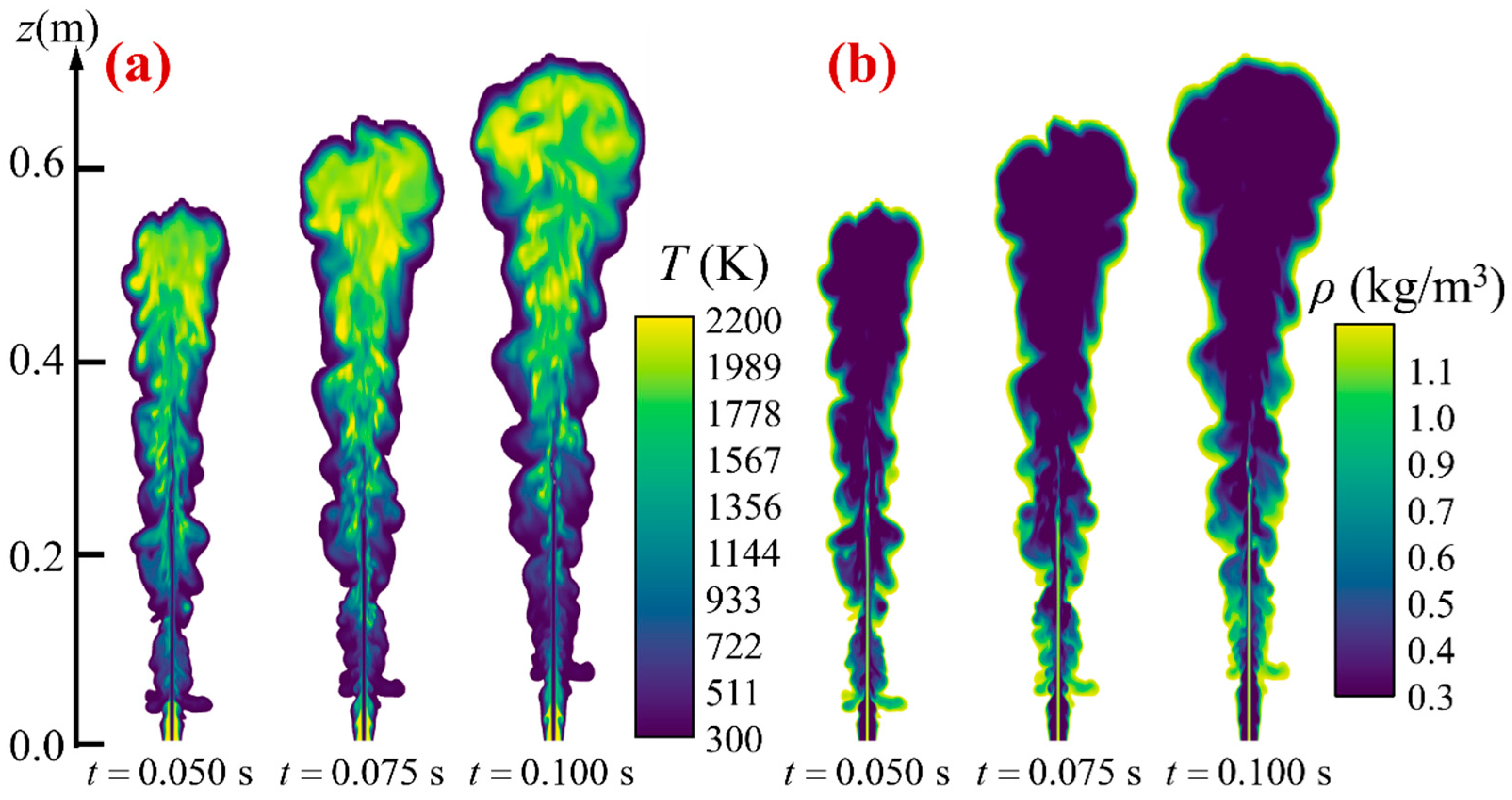
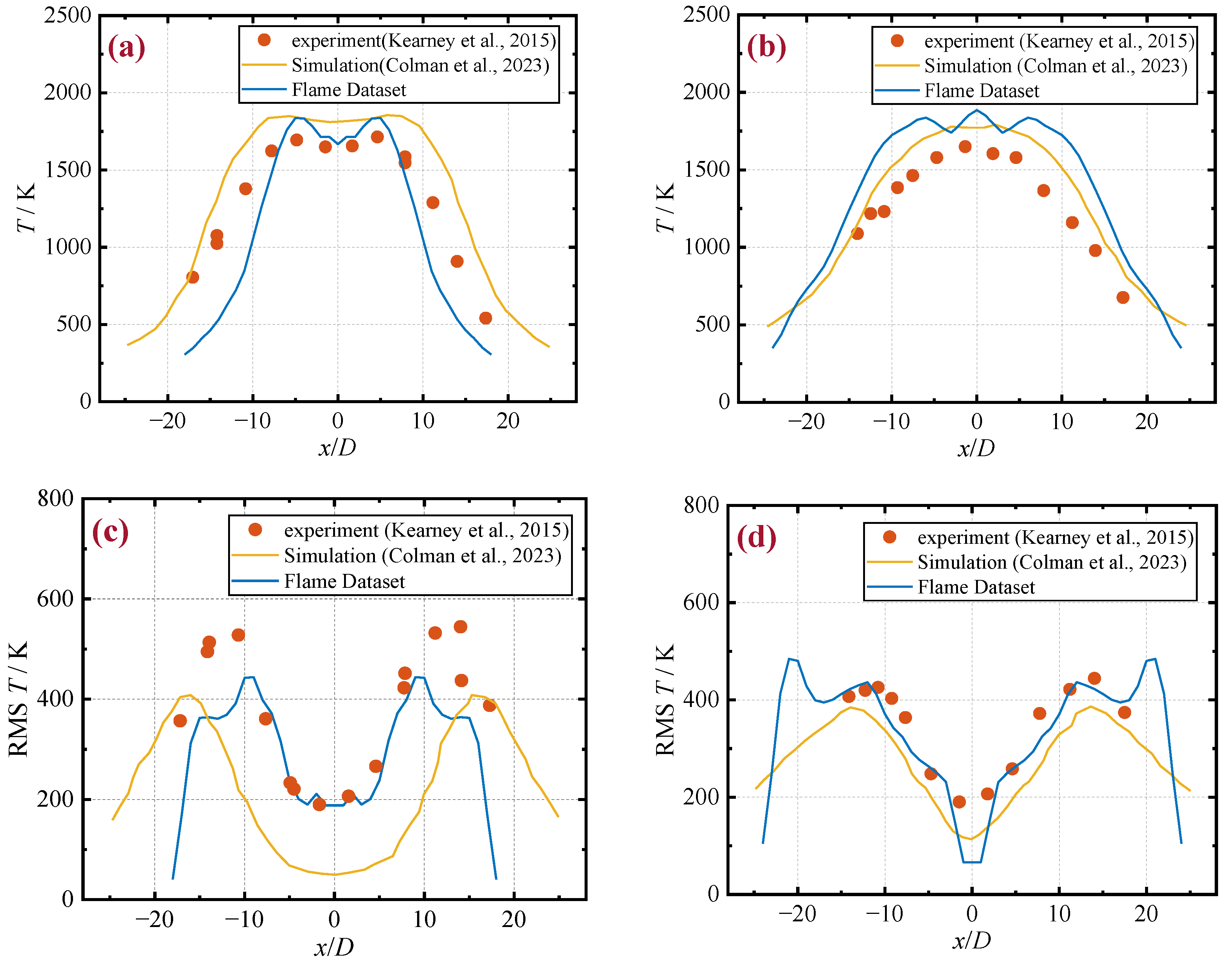
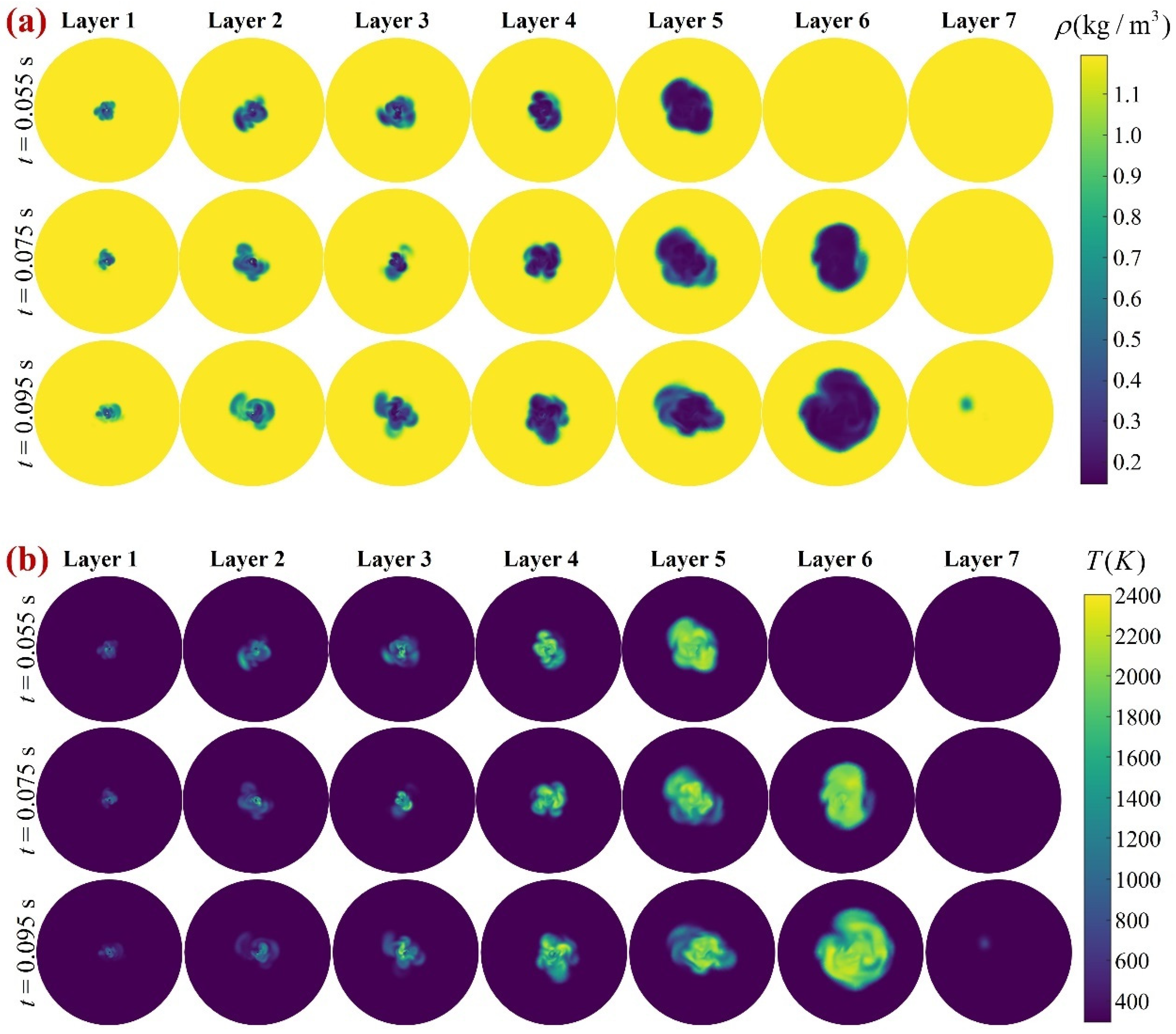
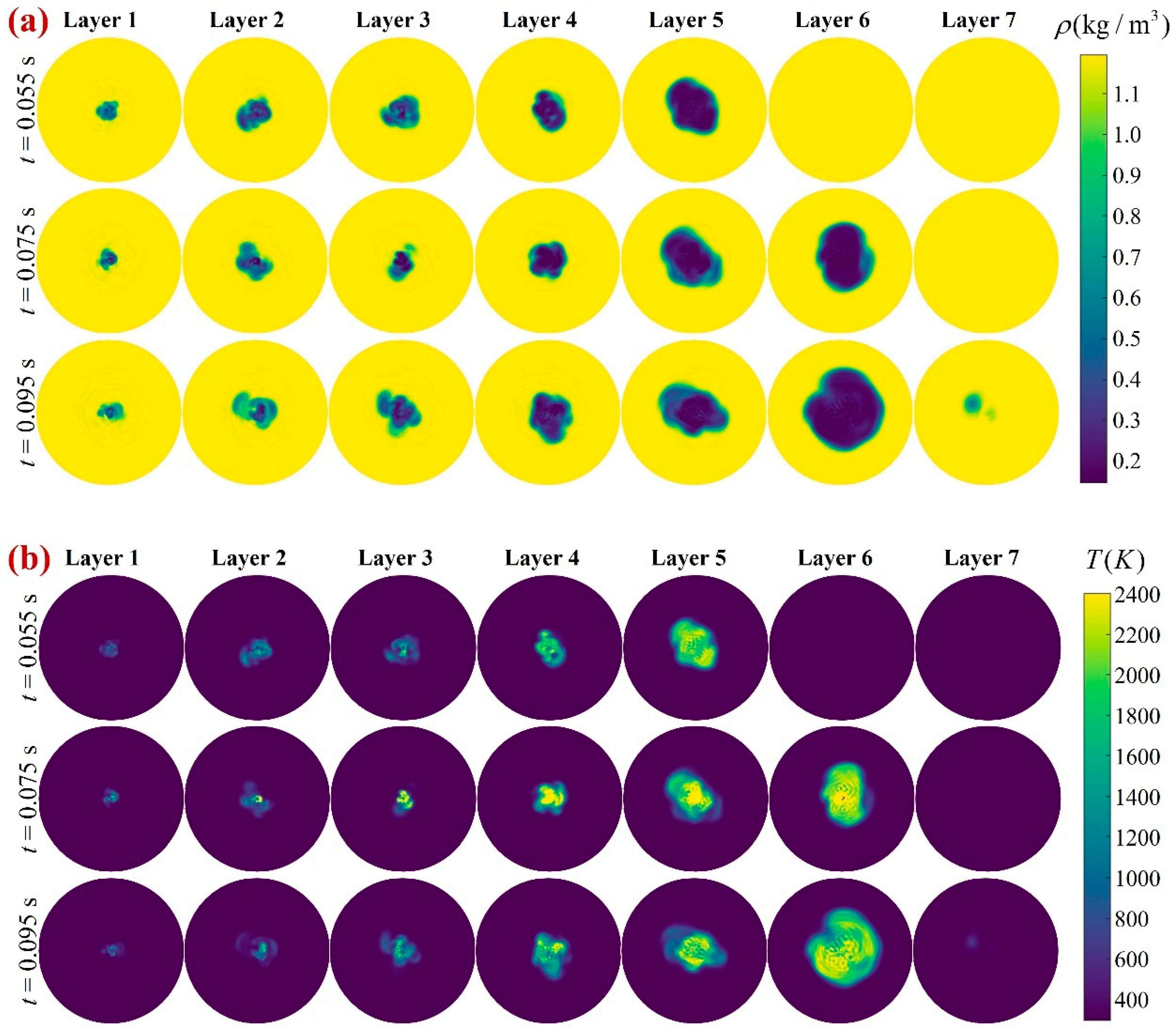
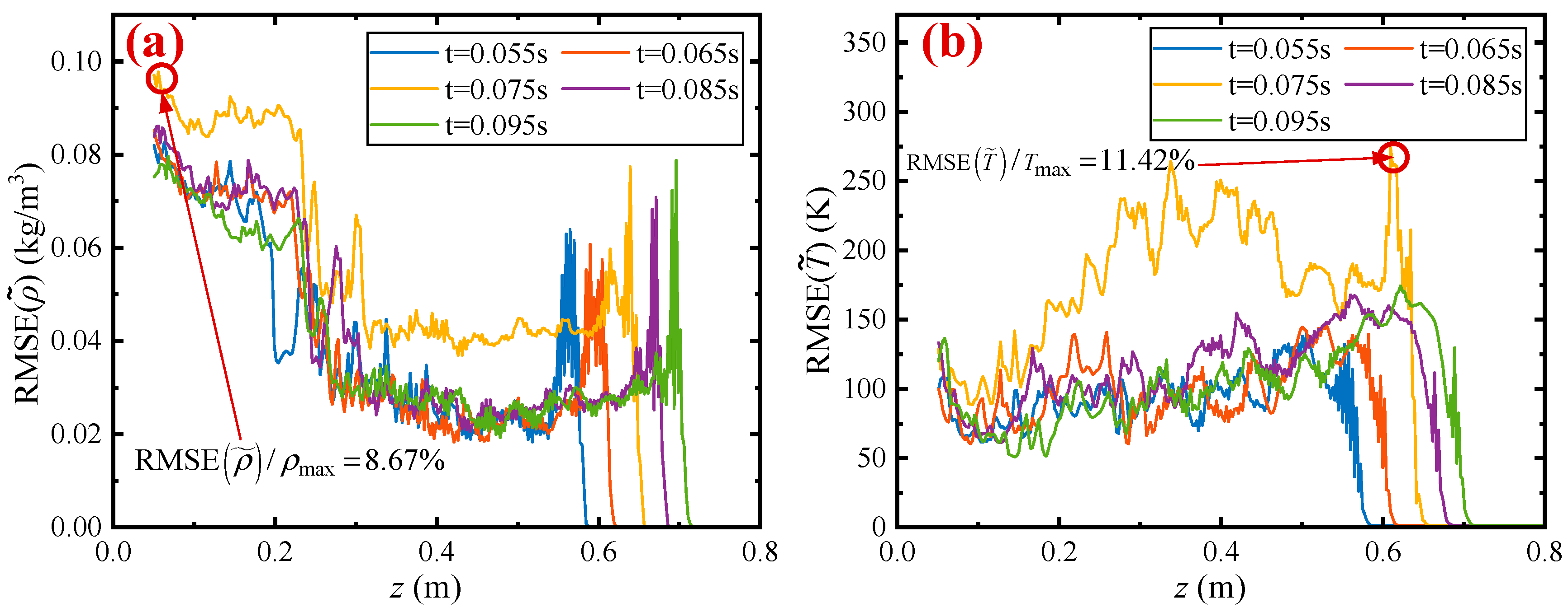
A double-cubic interpolation method for estimating the unknown orientation power spectral function in a polar coordinate system is proposed. The method’s applicability to 3D reconstruction performance is evaluated in terms of temperature and density fields, respectively, using the Sandia turbulent jet-diffusion flame as the study object. The results show that this method’s RMSE of the cross-section density for 3D reconstruction is below 0.1 kg/m³. In addition, the RMSE of the cross-section temperature is below 270 K.

(3)

Uncertainty analysis is performed by physical model-based flame reconstruction through k-d tree accelerated ray tracing. The relationship between the uncertainty of the 3D reconstructed temperature and density fields with the variance of the measurement is discussed for time asynchronous variance of 0.1 ms, 0.5 ms, and 1 ms, respectively. Overall, the uncertainties are positively correlated with the time asynchronous variance. For the time asynchronous variance of 1 ms, the density uncertainty of the 3D reconstruction is below 1.6 × 10⁻² kg/m³, and the temperature uncertainty is below 70 K, which means that the time asynchronous effect must be considered in experimental measurements.

Two aspects will be evaluated in the next study:

(a)

These preliminary results need to be further validated with more significant and more types of meshes. The current geometric model includes only standard flame CFD meshes. More orders of magnitude of grid parameters should be considered. Future work will address the accelerating effect of the k-d tree on the ray tracing process based on different orders of magnitude of nodes.

(b)

The flame model used in this paper is a standard Sandia turbulent jet diffusion flame. This is a common type of burner. Further discussion is needed to analyze the effects of time asynchrony for different types of combustors and at different Reynolds numbers. The analytical mechanism of these time asynchronies is a significant concern in the 3D reconstruction process. We will focus on the results of time asynchrony for different fuels, combustors, and Reynolds numbers.

References

1. Liu, H.; Wang, Y.; Yu, T.; Liu, H.; Cai, W.; Weng, S. Effect of carbon dioxide content in biogas on turbulent combustion in the combustor of micro gas turbine. Renew. Energy 2020, 147, 1299–1311. [Google Scholar] [CrossRef]
2. Grauer, S.J.; Unterberger, A.; Rittler, A.; Daun, K.J.; Kempf, A.M.; Mohri, K. Instantaneous 3D flame imaging by background-oriented Schlieren tomography. Combust. Flame 2018, 196, 284–299. [Google Scholar] [CrossRef]
3. Wei, J.F.; Ye, M.; Zhang, S.L.; Qin, J.; Haidn, O.J. Modeling of a 7-elements GOX/GCH4 combustion chamber using RANS with Eddy-Dissipation Concept model. Aerosp. Sci. Technol. 2020, 99, 105762. [Google Scholar] [CrossRef]
4. Wei, J.F.; Zhang, S.L.; Zuo, J.Y.; Qin, J.; Zhang, J.L.; Bao, W. Effects of combustion on the near-wall turbulence and performance for supersonic hydrogen film cooling using large eddy simulation. Phys. Fluids 2023, 35, 035112. [Google Scholar] [CrossRef]
5. Liu, H.C.; Huang, J.Q.; Li, L.; Cai, W.W. Volumetric imaging of flame refractive index, density, and temperature using background-oriented Schlieren tomography. Sci. China Technol. Sci. 2021, 64, 98–110. [Google Scholar] [CrossRef]
6. Jin, Y.; Zhang, W.; Song, Y.; Qu, X.; Li, Z.; Ji, Y.; He, A. Three-dimensional rapid flame chemiluminescence tomography via deep learning. Opt. Express 2019, 27, 27308–27334. [Google Scholar] [CrossRef] [PubMed]
7. Nygren, J.; Hult, J.; Richter, M.; Alden, M.; Christensen, M.; Hultqvist, A.; Johansson, B. Three-dimensional laser induced fluorescence of fuel distributions in an HCCI engine. Proc. Combust. Inst. 2002, 29, 679–685. [Google Scholar] [CrossRef]
8. Li, T.J.; Gao, P.; Zhang, C.X.; Yuan, Y.; Liu, D.; Shuai, Y.; Tan, H.P. Meshed axisymmetric flame simulation and temperature reconstruction using light field camera. Opt. Lasers Eng. 2022, 158. [Google Scholar] [CrossRef]
9. Li, T.J.; Li, S.N.; Yuan, Y.; Wang, F.Q.; Tan, H.P. Light field imaging analysis of flame radiative properties based on Monte Carlo method. Int. J. Heat Mass Transf. 2018, 119, 303–311. [Google Scholar] [CrossRef]
10. Li, T.J.; Yuan, Y.; Zhang, B.; Sun, J.; Xu, C.L.; Shuai, Y.; Tan, H.P. Experimental verification of three-dimensional temperature field reconstruction method based on Lucy-Richardson and nearest neighbor filtering joint deconvolution algorithm for flame light field imaging. Appl. Therm. Eng. 2019, 162, 114235. [Google Scholar] [CrossRef]
11. Li, T.J.; Zhang, C.X.; Liu, D. Simultaneously retrieving of soot temperature and volume fraction in participating media and laminar diffusion flame using multi-spectral light field imaging. Int. J. Therm. Sci. 2023, 193, 108472. [Google Scholar] [CrossRef]
12. Sanned, D.; Lindström, J.; Roth, A.; Aldén, M.; Richter, M. Arbitrary position 3D tomography for practical application in combustion diagnostics. Meas. Sci. Technol. 2022, 33, 125206. [Google Scholar] [CrossRef]
13. Nicolas, F.; Todoroff, V.; Plyer, A.; Le Besnerais, G.; Donjat, D.; Micheli, F.; Champagnat, F.; Cornic, P.; Le Sant, Y. A direct approach for instantaneous 3D density field reconstruction from background-oriented Schlieren (BOS) measurements. Exp. Fluids 2015, 57, 13. [Google Scholar] [CrossRef]
14. Liu, H.; Shui, C.; Cai, W. Time-resolved three-dimensional imaging of flame refractive index via endoscopic background-oriented Schlieren tomography using one single camera. Aerosp. Sci. Technol. 2020, 97, 105621. [Google Scholar] [CrossRef]
15. Choudhury, S.P.; Joarder, R. High-speed photography and background oriented Schlieren techniques for characterizing tulip flame. Combust. Flame 2022, 245, 112304. [Google Scholar] [CrossRef]
16. Cai, H.; Song, Y.; Ji, Y.; Li, Z.; He, A. Direct background-oriented Schlieren tomography using radial basis functions. Opt. Express 2022, 30, 19100–19120. [Google Scholar] [CrossRef]
17. Grauer, S.J.; Mohri, K.; Yu, T.; Liu, H.; Cai, W. Volumetric emission tomography for combustion processes. Prog. Energy Combust. Sci. 2023, 94, 101024. [Google Scholar] [CrossRef]
18. Yang, J.; Ma, Z.; Huang, L.; Li, X.; Jiang, H.; Yang, H.; Zhang, Y. Ignition measurement of non-premixed propane with varying co-flowing AIR through high-speed Schlieren stereoscopic colour imaging. Therm. Sci. Eng. Prog. 2022, 30, 101250. [Google Scholar] [CrossRef]
19. Wang, Y.F.; Zhu, X.M.; Jia, J.W.; Zhang, Y.H.; Liu, C.G.; Ning, Z.X.; Yu, D.R. Development of a circumferential-scanning tomography system for the measurement of 3-D plume distribution of the spacecraft plasma thrusters. Measurement 2023, 216, 112966. [Google Scholar] [CrossRef]
20. Gao, P.; Li, T.J.; Yuan, Y.; Dong, S.K. Numerical approaches and analysis of optical measurements of laser radar cross-sections affected by aero-optical transmission. Infrared Phys. Technol. 2022, 121, 104011. [Google Scholar] [CrossRef]
21. Gao, P.; Tao, D.X.; Yuan, Y.; Dong, S.K. A low-time complexity semi-analytic Monte Carlo radiative transfer model: Application to optical characteristics of complex spatial targets. J. Comput. Sci. 2023, 68, 101983. [Google Scholar] [CrossRef]
22. Zhang, J.Y.; Shaddix, C.R.; Schefer, R.W. Design of “model-friendly” turbulent non-premixed jet burners for C2+ hydrocarbon fuels. Rev. Sci. Instrum. 2011, 82, 074101. [Google Scholar] [CrossRef] [PubMed]
23. Torres-Monclard, K.; Gicquel, O.; Vicquelin, R. A quasi-monte carlo method to compute scattering effects in radiative heat transfer: Application to a sooted jet flame. Int. J. Heat Mass Transf. 2021, 168, 120915. [Google Scholar] [CrossRef]
24. Tian, L.; Lindstedt, R.P. On the impact of differential diffusion between soot and gas phase species in turbulent flames. Combust. Flame 2023, 251, 112684. [Google Scholar] [CrossRef]
25. Rodrigues, P.; Franzelli, B.; Vicquelin, R.; Gicquel, O.; Darabiha, N. Coupling an LES approach and a soot sectional model for the study of sooting turbulent non-premixed flames. Combust. Flame 2018, 190, 477–499. [Google Scholar] [CrossRef]
26. Colman, H.M.; Darabiha, N.; Veynante, D.; Fiorina, B. A turbulent combustion model for soot formation at the LES subgrid-scale using virtual chemistry approach. Combust. Flame 2023, 247, 112496. [Google Scholar] [CrossRef]
27. Kearney, S.P.; Guildenbecher, D.R.; Winters, C.; Farias, P.A.; Grasser, T.W.; Hewson, J.C. Temperature, Oxygen, and Soot-Volume-Fraction Measurements in a Turbulent C2H4-Fueled Jet Flame; Sandia National Lab. (SNL-NM): Albuquerque, NM, USA, 2015. [Google Scholar]
28. Gori, G.; Guardone, A. VirtuaSchlieren: A hybrid GPU/CPU-based Schlieren simulator for ideal and non-ideal compressible-fluid flows. Appl. Math. Comput. 2018, 319, 647–661. [Google Scholar] [CrossRef]
29. Amjad, S.; Karami, S.; Soria, J.; Atkinson, C. Assessment of three-dimensional density measurements from tomographic background-oriented Schlieren (BOS). Meas. Sci. Technol. 2020, 31, 114002. [Google Scholar] [CrossRef]
Figure 1. Schematic diagram of 3D reconstruction of background-oriented Schlieren tomography system.
Fire 06 00417 g001
Figure 2. Turbulent flame field for a typical combustion time. (a) temperature. (b) density.
Fire 06 00417 g002
Figure 3. Comparison of mean and RMS temperature with experiment [27] and simulation [26]. (a) mean temperature, z/D = 134. (b) RMS temperature, z/D = 134. (c) mean temperature, z/D = 165. (d) RMS temperature, z/D = 165.
Fire 06 00417 g003
Figure 4. Time complexity analysis of 3D reconstruction performed by the BOST system. (a) Time complexity corresponding to different positions. (b) Normalized probability density distribution function of the time complexity.
Fire 06 00417 g004
Figure 5. Temperature and density information of the Sandia flame observed at different moments. Height layers 1 to 7 correspond to heights of 0.1 to 0.7 m, respectively, in steps of 0.1 m. (a) Density field, (b) temperature field.
Fire 06 00417 g005
Figure 6. Camera’s background-oriented Schlieren deflection angle for different viewing azimuths.
Fire 06 00417 g006
Figure 7. Three-dimensional (3D) reconstruction of the temperature and density fields of the Sandia flame based on a power spectral density estimation method in a polar coordinate system. Height layers 1 to 7 correspond to heights of 0.1 to 0.7 m, respectively, in steps of 0.1 m. (a) Density field, (b) temperature field.
Fire 06 00417 g007
Figure 8. Mean root-mean-square error of slices reconstructed in three dimensions for different height layers. (a) Density field, (b) temperature field.
Fire 06 00417 g008
Figure 9. Effect of time asynchrony on 3D reconstruction in the BOST system with a combustion time of 0.075 s. (a) Density reconstruction compared to fully time-synchronized slice-averaged deviation values. (b) Temperature reconstruction compared to fully time-synchronized slice-averaged deviation values. (c) Mean density uncertainty for different slices. (d) Mean temperature uncertainty for different slices. (e) Density and temperature reconstruction uncertainties for height layers 1 to 3 corresponding to heights of 0.1 m, 0.3 m and 0.5 m, respectively. The selected time variance is 1 ms. (f) Frequency distribution plot of camera time asynchrony over 50 measurements.
Fire 06 00417 g009