Simplified Interfacial Area Modeling in Polydisperse Two-Phase Flows under Explosion Situations

Abstract

The aim of the present work is to account for polydisperse effects in a two-phase flow with a simple and fast method. Polydisperse two-phase flows arise in numerous applications. Fire sprinkler systems are relevant examples as they release clouds of polydisperse droplets. Another relevant example is the polydisperse two-phase flow created by the detonation of an explosive charge surrounded by a liquid layer. In such a situation, material interfaces are initially present and the created two-phase flow consists of a carrier gas phase and a liquid phase involving many droplets of various sizes. Spherical particles or droplets are usually assumed in two-phase flow computations. When dealing with explosion situations involving both dense and dilute flow regimes, multiple particle diameters can be addressed but at the price of introducing as many additional equations that describe mass, momentum and energy balance of the various particle classes. Consequently, the computation time needed to address numerical resolution increases tremendously. Under explosion situations involving many particle diameters, the method becomes intractable and is usually reduced to a single diameter, which is often insufficient. A simplified approach is developed in the present work to account for a substantial number of particles of different sizes with few extra computational cost. The approach is said to be simplified as a single velocity and a single temperature are considered for all the spherical particles, regardless of their diameters. This type of modeling seems apt for the target explosion situations. The focus is placed on the interfacial area, which is the main parameter involved in the coupling of the two phases. In the present work, Gamma-like continuous probability distributions are considered to address the various sizes of particles. The effects of the size distribution are only summarized in the specific interfacial area, yielding consequently few code modifications while taking into account the polydisperse aspect of the two-phase flow.

1. Introduction

Many two-phase flows involve a very large number of liquid or solid particles per unit volume (typically ${10}^{12}$ particles $·{\mathrm{m}}^{-3}$) having a significant impact on the behavior of the flow, as a result of interactions. Such two-phase flows appear in various contexts, such as the transport of solid particles by air (Marble, 1963 [1]), the collection of ice on buildings and aircraft structures (Lewis and Brun, 1956 [2], Gelder et al., 1956 [3]), or fluidized beds and other two-phase flow phenomena of interest in chemical processing (Torobin and Gauvin, 1959 [4]). Other relevant examples are fire sprinkler systems that release clouds of polydisperse droplets, fluid-droplet sprays that are of particular interest for applications involving combustion (Williams, 1958 [5]), and fuel suspensions resulting from explosion situations. This last case involves combustion as well and is of particular interest in the present contribution.

Whether in liquid sprays or when a liquid layer is set in motion by the detonation of an explosive charge, many liquid droplets of various sizes are created and consequently involve a large exchange surface with the gas phase. Determination of the interfacial area is a key problem in combustion and two-phase flow modeling (Drew and Passman, 2006 [6]). An illustrative example of a liquid layer set in motion by an explosive charge is presented in Figure 1.

The liquid phase is said to be polydisperse as it contains a substantial number of droplets of different sizes, having major effects on the two-phase flow. Various methods are available to address multi-dimensional computations of polydisperse flows. See for instance [7,8,9,10,11,12,13] in the context of polydisperse sprays where the droplets are diluted in a carrier phase. When dealing with explosion situations, such as the one of Figure 1, the liquid layer transforms to a cloud of polydisperse droplets as well. However, material interfaces are initially present and bring out additional numerical difficulties.

One way to account for multiple sizes of particles, or droplets in the present explosion context where both dense and dilute flow regimes occur, is to address each class of particles with its own set of balance equations (mass, momentum, total energy, and specific number of particles). In the present work, a class of particles represents a population of spherical particles having a distinct size (radius). Each class of particles can be described by its own radius, velocity, temperature, specific number and specific interfacial area that can be easily determined, provided that the particles are supposed to be spherical. This approach appears ideal and appealing but becomes intractable when dealing with real explosion situations involving a very large number of classes of particles and consequently an even larger number of additional equations, tremendously increasing the computation time needed to address numerical simulations. In such a case, the method is usually reduced to a single or few classes of particles, which is often insufficient.

The present paper attempts to reduce substantially the simulation time while increasing the accuracy of the solution. Multiple approaches have been developed to address polydisperse effects without the burden of introducing many additional balance equations. For example, Fan et al. (2004) [14] consider a population balance equation (PBE), coupled to the continuity and momentum balance equations with the help of the direct quadrature method of moments (DQMOM). This method seems to be the most popular to deal with polydisperse effects. However it is restricted to dilute flows, where the volume fraction of the dispersed phase as well as related terms are neglected. The flow model is in the same sense an extended version of Marble’s model (1963) [1]. This method then appears unable to account for initial material interfaces, such as the initial liquid-gas interface depicted in Figure 1. In such a situation, a material interface is present and the flow ranges from dense to dilute concentration of particles. The DQMOM method is consequently unsuitable to address the present target applications involving initial material interfaces. However, it appears well-suited to deal with spray flows, Fox et al. (2008) [15].

Baer-and-Nunziato-type (1986) [16] two-phase flow models are then preferred. Various variants are available, such as Saurel et al.’s (2003, 2017) [17,18]. In the present work, unlike the DQMOM method, the liquid phase is described by a single velocity and a single temperature but multiple classes of particles. This simplification has been used for instance in Olmos et al. (2001) [19] in the context of bubble-column reactors, where the different classes of particles are convected with the same mean algebraic velocity. It may appear contradictory at first glance but implies that the essential of the polydisperse effects is addressed through the specific interfacial area which accounts for a whole spectrum of radius distributions. In the present explosion context, this assumption appears appropriate as timescales related to velocity relaxation are small. Moreover, such a modeling appears realistic when the liquid phase reaches the saturation temperature which is independent of the sizes of the droplets. The polydisperse character of the liquid phase is only summarized in the specific interfacial area, and only two phases are needed, i.e., the gas phase and the liquid phase that is made of polydisperse droplets. Consequently, only two sets of balance equations are required and the computation time requested to perform a simulation is comparable to the one needed by a conventional computation, considering a unique droplet size in a control volume.

A droplet size distribution is needed nonetheless. Many experimental studies aim to describe the size distribution in various applications. Recent works include for instance Chandrakar et al. (2016) [20] where the influence of aerosol concentration on a cloud-droplet size distribution is investigated in a laboratory chamber, or Rousseau et al. (2021) [21] where spray combustion is studied with the help of an experimental test rig. Some theoretical studies attempt to reproduce favorable experimental data. For instance, Carrica et al. (1999) [22] used a statistical description of two-phase flows based on the Boltzmann theory of dispersed gases, and described a bubble distribution function with the help of the bubble mass, position and time. Li and Li (2003) [23] proposed a droplet size distribution model based on the concept of the maximization of entropy generation during the liquid atomization process. Zhang et al. (2019) [24] developed a theoretical framework based on the contact and the coalescence of droplets.

In the present paper, the droplet size distribution is based on a continuous probability distribution. Many mathematical functions are available and used to address particle size distribution (Yoon, 2005 [25], Igel and Van Den Heever, 2017 [26], Urbán and Józsa, 2018 [27], Hareli et al., 2021 [28] to cite a few). The commonly used size distribution functions in fluid dynamics include the Normal, Log-Normal, Nukiyama–Tanasawa, Rosin–Rammler, Beta, modified Beta and Gamma-type distributions. Discussions about these size distribution functions can be found in Ge (2006) [29] for instance. The proposed method is presented with the help of Gamma-type distributions but may be used with various functions.

The paper is organized as follows. Section 2 presents the two-phase model. Viscous drag interaction effects, having a major impact on the two-phase flow, are introduced in Section 3. Section 4 presents the proposed method and attempts to address, through a simple size distribution function, the polydisperse effects of the liquid phase. Computational examples are provided in Section 5.

2. Flow Model

The model of Baer and Nunziato (1986) [16] is based upon a mixture evolving in total disequilibrium. It is based upon the inviscid Euler equations for each pure phase. The balance equations for phases 1 and 2 are,

$$\left\{\begin{array}{c}\begin{array}{cc}\hfill & \frac{\partial {\alpha }_1}{\partial t}+u_I\frac{\partial {\alpha }_1}{\partial x}=\mu (p_1-p_2),\hfill \\ \hfill & \frac{\partial \left({\alpha }_1{\rho }_1\right)}{\partial t}+\frac{\partial \left({\alpha }_1{\rho }_1{u}_1\right)}{\partial x}=0,\hfill \\ \hfill & \frac{\partial \left({\alpha }_1{\rho }_1{u}_1\right)}{\partial t}+\frac{\partial \left({\alpha }_1\left({\rho }_1{u}_1^2+p_1\right)\right)}{\partial x}=p_I\frac{\partial {\alpha }_1}{\partial x}+\lambda \left(u_2-u_1\right),\hfill \\ \hfill & \frac{\partial \left({\alpha }_1{\rho }_1{E}_1\right)}{\partial t}+\frac{\partial \left({\alpha }_1\left({\rho }_1{E}_1+p_1\right)u_1\right)}{\partial x}=p_I{u}_I\frac{\partial {\alpha }_1}{\partial x}-\mu p_I^{\prime }(p_1-p_2)+\lambda u_I^{\prime }\left(u_2-u_1\right),\hfill \\ \hfill & \frac{\partial \left({\alpha }_2{\rho }_2\right)}{\partial t}+\frac{\partial \left({\alpha }_2{\rho }_2{u}_2\right)}{\partial x}=0,\hfill \\ \hfill & \frac{\partial \left({\alpha }_2{\rho }_2{u}_2\right)}{\partial t}+\frac{\partial \left({\alpha }_2\left({\rho }_2{u}_2^2+p_2\right)\right)}{\partial x}=p_I\frac{\partial {\alpha }_2}{\partial x}-\lambda \left(u_2-u_1\right),\hfill \\ \hfill & \frac{\partial \left({\alpha }_2{\rho }_2{E}_2\right)}{\partial t}+\frac{\partial \left({\alpha }_2\left({\rho }_2{E}_2+p_2\right)u_2\right)}{\partial x}=p_I{u}_I\frac{\partial {\alpha }_2}{\partial x}+\mu p_I^{\prime }(p_1-p_2)-\lambda u_I^{\prime }\left(u_2-u_1\right),\hfill \\ \hfill & \frac{\partial N_2}{\partial t}+\frac{\partial \left(N_2{u}_2\right)}{\partial x}=0.\hfill \end{array}\hfill \end{array}\right.$$

(1)

The notations are conventional in the two-phase flow literature. A frame of reference $\left(x\right)$ is chosen and the time variable is denoted by t. ${\alpha }_k$, ${\rho }_k$, $p_k$, $E_k=e_k+\frac{1}{2}{u}_k^2$ denote respectively the volume fraction, density, pressure and total energy of phase k. $e_k$ represents the internal energy and $u_k$ represents the center of mass velocity of phase k. $N_2$ represents the specific number of particles, i.e., the total number of particles per unit volume. In the rest of the paper, the carrier gas phase will then be indexed by 1 and the liquid phase by 2. The mixture internal energy is defined as $e=\sum Y_k{e}_k$ where $Y_k=\left({\alpha }_k{\rho }_k\right)/\rho$ denotes the mass fraction of phase k. The mixture density and pressure are defined as $\rho =\sum {\alpha }_k{\rho }_k$ and $p=\sum {\alpha }_k{\rho }_k$.

Equation system (1) is a two-phase model for mixture flows evolving in pressure, velocity and temperature disequilibria. The choice of interfacial average velocities $u_I$ and pressures $p_I$ was originally expressed with the relations $u_I=u_2\mathrm{and}{p}_I=p_1$, the symmetric choice $u_I=u_1\mathrm{and}{p}_I=p_2$, being possible as well. More general and symmetric estimates have been proposed by Saurel et al. (2003) [17],

$$\left\{\begin{array}{c}\begin{array}{ccccc}\hfill u_I& =u_I^{\prime }+sgn\left(\frac{\partial {\alpha }_1}{\partial x}\right)\frac{p_2-p_1}{Z_1+Z_2},\hfill & \hfill & \mathrm{with}{u}_I^{\prime }\hfill & \hfill =\frac{Z_1{u}_1+Z_2{u}_2}{Z_1+Z_2},\\ \hfill p_I& =p_I^{\prime }+sgn\left(\frac{\partial {\alpha }_1}{\partial x}\right)\frac{\left(u_2-u_1\right)Z_1{Z}_2}{Z_1+Z_2}\hfill & \hfill & \mathrm{with}{p}_I^{\prime }\hfill & \hfill =\frac{Z_1{p}_2+Z_2{p}_1}{Z_1+Z_2},\end{array}\hfill \end{array}\right.$$

(2)

where $Z_k={\rho }_k{c}_k$ is the acoustic impedance and $c_k$ is the speed of sound of fluid k. This latter is provided by a convex equation of state for each phase. The analysis which has led to these estimates is based upon a homogenization method developed by Abgrall and Saurel (2003) [30]. Equations (1) have been extended to 3D in Franquet and Perrier (2012) [31].

The first equation of (1) is non-conservative and represents the transport of the first volume fraction ${\alpha }_1$ at interfacial velocity $u_I$. During the advection stage, volume variations caused by pressure differences between the phases appear through the relaxation term $\mu (p_1-p_2)$, where $\mu$ controls the rate at which pressure equilibrium is reached. The above-mentioned analysis provided this coefficient as well $\mu =\frac{A_I}{Z_1+Z_2}$ where $A_I$ represents the specific interfacial area of the mixture. For instance, when dealing with a cloud of liquid droplets of a single radius $R_2$, the specific interfacial area is $A_I=\frac{3{\alpha }_2}{R_2}$. The volume variations of the phases are then directly proportional to the pressure difference between the phases and the speed at which the equilibrium is reached is controlled by the $\mu$ coefficient. This latter depends only upon the acoustic impedance of the phases and upon the specific interfacial area $A_I$. The second and fifth equations of (1) describe mass balance of the corresponding phase while the third and sixth equations are related to their momentum balance. These last two relations are non-conservative. The velocity relaxation terms on the right-hand side of the momentum equations read $\pm \lambda \left(u_2-u_1\right)$, where $\lambda$ is the product of the specific interfacial area with the drag coefficient. $\lambda$ is a positive function (or tensor if there are more than two fluids). It is involved in the viscous drag force between the two phases and controls the rate at which velocities tend towards equilibrium. The non-conservative term $p_I\frac{\partial {\alpha }_1}{\partial x}$ represents the pressure force acting at the liquid droplet cloud boundaries with $p_I$ denoting the interfacial pressure given by Equation (2). This non-conservative term represents a “differential drag force” as its amplitude is high in zones of high volume gradients and vanishes when the volume fraction is uniform. It has been shown in Chiapolino and Saurel (2020) [32] that this term is of main importance in the formation of particle jets in the explosion situation depicted in Figure 1. The fourth and seventh equations of (1) describe the energy balance of phase k. Those latter ones are non-conservative as well due to the presence of the term $p_I{u}_I\frac{\partial {\alpha }_k}{\partial x}$ and the relaxation terms on the right-hand side. Finally, the last equation describes the conservation of the specific number $N_2$ of liquid particles (droplets). This equation is conservative as fragmentation effects are not considered in the present work. Thermal exchange effects and mass transfer have been omitted as well for the sake simplicity.

Equation system (1) considers mixtures in pressure, velocity and temperature disequilibria. Its extension to more than two phases is possible [33]. It is able to deal with material interfaces encountered for instance at the early times of the explosion situation depicted in Figure 1, as well as two-phase suspensions occurring at later times. For the target explosion situations, the two-phase equation system (1) of Saurel et al. (2003) [17], variant of Baer and Nunziato’s (BN) model (1986) [16], is consequently preferred over the model of Marble (1963) [1] or the DQMOM formulation [14,15,34], suitable only in the limit of disperse flows. Such formulations are indeed suitable for dilute spray flows but cannot address resolved-interface situations where material interfaces separate two pure or nearly pure media.

The two-phase equation system (1) ensures the satisfaction of the interface conditions through the non-conservative terms and the associated interfacial variables (Saurel and Pantano, 2018 [35]). Equation system (1) is indeed able to fulfill the expected interface condition of mechanical equilibrium (continuity of pressures and normal velocities) in the two limits, $\lambda ,\mu =0$ and $\lambda ,\mu \to \infty$. In the first option, the interface conditions are ensured by the non-conservative terms as the interfacial variables in Equation (2) model contact interface conditions as general solutions of local Riemann problems. This method has been used, for example, by Layes and Le Métayer (2007) [36] to study shock interaction with a gas bubble. The two-phase formulation is also able to deal with permeable interfaces (boundaries of bubbles or droplets clouds). For instance, it has been used to address permeable granular interfaces by Saurel et al. (2014) [37], who extended (1) to account for granular effects. The second option relies on stiff mechanical relaxation. In this limit the mixture evolves with a single pressure and a single velocity. This approach was proposed by Saurel and Abgrall (1999) [38] in a splitting formulation where the hyperbolic part of (1) is solved during a time step in the absence of source terms, followed by pressure and velocity relaxation steps with sources $\mu (p_1-p_2)$ and $\lambda \left(u_2-u_1\right)$ respectively, with both $\lambda ,\mu \to \infty$.

Indeed, relaxation phenomena can be added depending upon the flow condition of the multiphase medium and may yield total or partial equilibrium depending upon the rate at which the corresponding equilibrium is supposed to be reached. For example, instantaneous pressure equilibrium may be found whereas velocities remain in disequilibrium. These circumstances are typical of explosion situations, as typical timescales associated with the pressure equilibrating process are small [33,39], and are of particular interest of the present work. Note that such an instantaneous pressure relaxation is not equivalent to strict pressure equilibrium that yields non-hyperbolic or conditionally hyperbolic models. Details of stiff relaxation solvers can be found in Le Métayer et al. (2013) [40] for instance.

Under the form (1), the formulation is restricted to two phases, i.e., a carrier gas phase (indexed 1) and a liquid phase (indexed 2) made of a single class of $N_2$ droplets of radius $R_2$. Equation system (1) can be extended to account for multiple classes of droplets with the help of as many additional sets of balance equations. In such a case, each class of droplet is described by its own radius, velocity, temperature, specific number and specific interfacial area. However, the present paper attempts to account for the polydisperse character of the liquid phase with a simplified method. As only flow situations involving pressure equilibrium between the gas and liquid phases are of interest in the present work, the polydisperse aspect of the liquid droplets impacts only the viscous drag force between the two phases through the specific interfacial area $A_I$. The viscous drag effects are addressed hereafter.

3. Viscous Drag

For the sake of clarity, computation of the viscous drag force is presented in the context of a single class of particles. In a control volume, the liquid phase is then made of $N_2$ droplets of a single radius $R_2$. Polydisperse effects will be accounted for later through the specific interfacial area $A_I$. The viscous drag parameter $\lambda$ present in Equation system (1) controls the rate at which velocity equilibrium is reached between the gas and liquid phases. The $\lambda \left(u_2-u_1\right)$ term represents the viscous drag force and $\lambda u_I^{\prime }\left(u_2-u_1\right)$ the power of this force (per unit volume). In the following, this force is denoted as $N_2{F}_{1\to 2}$ where $N_2$ represents the specific number of droplets. For the sake of simplicity the droplets are considered spherical in this work and viscous drag effects are treated via the following Stokes relation,

$$F_{1\to 2}=6\pi {\mu }_1{R}_2\left(u_1-u_2\right),$$

(3)

where $R_2$ is the radius of the droplets and ${\mu }_1$ the dynamic viscosity of the carrier phase. The particle Reynolds number is now introduced,

$$R{e}_2=\frac{2R_2{\rho }_1|u_2-u_1|}{{\mu }_1}.$$

(4)

It is important to note that such viscous drag representation is only valid for low Reynolds numbers. In such conditions the viscous drag coefficient reads $C_d=\frac{24}{R{e}_2}$. With the help of the previous relations, the viscous drag force can be written concisely as,

$$F_{1\to 2}=\frac{C_d{R}_2^2\pi {\rho }_1}{2}|u_2-u_1|\left(u_1-u_2\right).$$

(5)

However, in order to extend the present viscous drag law to higher Reynolds numbers, the viscous drag coefficient is reconsidered to account for turbulent effects following Naumann and Schiller (1935) [41],

$$C_d=\left\{\begin{array}{c}\begin{array}{ccc}\frac{24}{R{e}_2}\left(1+0.15R{e}_2^{0.687}\right)\hfill & \hfill & \mathrm{if}R{e}_2<800,\hfill \\ 0.438\hfill & \hfill & \mathrm{otherwise}.\hfill \end{array}\hfill \end{array}\right.$$

(6)

As the droplets are considered spherical with a radius $R_2$, the specific number of droplets reads

$$N_2=\frac{{\alpha }_2}{\frac{4}{3}\pi R_2^3},$$

(7)

and the total viscous drag force in a control volume becomes

$$N_2{F}_{1\to 2}=\frac{3}{8R_2}{\alpha }_2{C}_d{\rho }_1|u_2-u_1|\left(u_1-u_2\right),$$

(8)

that is to say,

$$N_2{F}_{1\to 2}=\lambda \left(u_1-u_2\right)\mathrm{with}\lambda =\frac{3}{8R_2}{\alpha }_2{C}_d{\rho }_1|u_2-u_1|.$$

(9)

It is however more convenient to express Equation (9) in terms of specific interfacial area $A_I$. The droplets being spherical, the specific interfacial area reads,

$$A_I=4\pi R_2^2{N}_2.$$

(10)

The combination of Equations (7) and (10) yields,

$$A_I=\frac{3{\alpha }_2}{R_2}.$$

(11)

The viscous drag parameter $\lambda$ is consequently expressed as,

$$\lambda =\left(\frac{1}{8}{C}_d{\rho }_1|u_2-u_1|\right)\times A_I.$$

(12)

Relation (12) is used to compute the viscous drag effects between the carrier gas phase 1 and the liquid phase 2. Turbulent effects are summarized through the $C_d$ coefficient, present in the first term of Equation (12), and is determined with the help of Equation (6). It depends on the particle Reynolds number (4) which itself depends on the radius $R_2$ of the droplets. This latter is determined by Equation (7), as the number of droplets $N_2$ as well as the volume fraction of the liquid phase ${\alpha }_2$ are known from the balance equations of (1). The size of the droplets is addressed through the specific interfacial area $A_I$, present as the second term of Equation (12), and determined via Equation (11).

In the following section, multiple sizes of droplets are addressed via a simplified method that accounts for a whole spectrum of particle radii through the specific interfacial area $A_I$, that is reconsidered. Computation of $A_I$ relies on a continuous probability distribution and yields only few code modifications. Depending on the context multiple distribution functions can be used as long as their distribution moments are available, as will be seen hereafter.

4. Polydisperse Particles

Computation of the viscous drag force, with polydisperse droplets, is based on the previous monodisperse relations. However the specific interfacial area $A_I$ is adjusted to account for the multiple droplet sizes. The drag force is computed via Equation (9) with the help of the $\lambda$ coefficient determined by Equation (12). This later depends on the specific interfacial area $A_I$ that will now be reconsidered.

4.1. General Relations

Two additional variables are introduced to deal with the multiple classes of particles. Those are ${\alpha }_{2,k}$ and $N_{2,k}$ that denote respectively the volume fraction and the specific number (per unit volume) of particles of the kth class. Recall that index 2 denotes the liquid phase composed of spherical particles, or droplets in the present context.

4.1.1. Liquid Volume Fraction and Number of Particles

The particles being spherical, the following relation appears,

$${\alpha }_{2,k}=\frac{4}{3}\pi R_{2,k}^3{N}_{2,k}.$$

(13)

Moreover, the volume fraction of the liquid phase ${\alpha }_2$ is defined as the sum of the volume fractions ${\alpha }_{2,k}$ constituting the liquid phase,

$${\alpha }_2=\sum _{k=1}^{N_{classes}}{\alpha }_{2,k},$$

(14)

where $N_{classes}$ is the number of classes of particles. In the present context, the volume fractions ${\alpha }_{2,k}$ of the various classes of droplets depend on the various radii $R_{2,k}$. As the liquid volume fraction ${\alpha }_2$ is the sum of the ${\alpha }_{2,k}$ volume fractions, the following relation arises:

$${\alpha }_2={\int }_0^{\infty }{\alpha }_{2,k}\left(R_2\right)d{R}_2.$$

(15)

The volume fraction ${\alpha }_{2,k}$, describing the volume occupied by the class k of particles in the liquid phase (2), is defined by Equation (13) involving the specific number $N_{2,k}$ of particles of the kth class. In order to account for multiple sizes of particles, a continuous probability distribution is addressed in the following. To this end, the probability $P\left(R_2\in [a,b]\right)$ is introduced and corresponds to the probability for the radius of the particles to belong in the interval $[a,b]$. This probability reads,

$$P\left(R_2\in [a,b]\right)={\int }_a^{b}f\left(R_2\right)d{R}_2,$$

(16)

where f is the probability density function (PDF). It is important to emphasize that the PDF specifies the probability of radius $R_2$ falling within a specific range of values, as opposed to taking on any one value. With the help of Equation (16) the specific number of particles having a radius in the interval $[a,b]$ is expressed as,

$$N\left(R_2\in [a,b]\right)=N_{2}P\left(R_2\in [a,b]\right)=N_2{\int }_a^{b}f\left(R_2\right)d{R}_2,$$

(17)

with $N_2$ the specific total number of liquid particles, all sizes included. Note that a probability density function satisfies the properties:

$$f\left(R_2\right)\ge 0,\forall R_2\mathrm{and}{\int }_{-\infty }^{+\infty }f\left(R_2\right)d{R}_2=1.$$

(18)

However, in the present two-phase context, the interval is reduced to $R_2\in [0,+\infty ]$. As a result, the total number of particles $N_2$ is recovered in the $[0,+\infty ]$ interval,

$$N\left(R_2\in [0,+\infty ]\right)=N_2{\int }_0^{+\infty }f\left(R_2\right)d{R}_2=N_2.$$

(19)

The specific number $N_{2,k}$ of particles of the kth class, present in Equation (13), is then to be expressed with a range of values for $R_2$. Consequently, an infinitesimal interval $[R,R+dR]$ is considered. Equation (13) is then used under the form,

$${\alpha }_{2,k}\left(R_2\right)=\frac{4}{3}\pi R_2^{3}N\left(R_2\in [R,R+dR]\right).$$

(20)

Equation (20) is now introduced in (15),

$${\alpha }_2={\int }_0^{\infty }\frac{4}{3}\pi R_2^{3}N\left(R_2\in [R,R+dR]\right)d{R}_2.$$

(21)

Then, Expression (17) is embedded in this last relation and yields

$${\alpha }_2={\int }_0^{\infty }\left(\frac{4}{3}\pi R_2^3{N}_2{\int }_R^{R+dR}f\left(R_2\right)d{R}_2\right)d{R}_2.$$

(22)

The second integral term is now analyzed:

$${\int }_R^{R+dR}f\left(R_2\right)d{R}_2=F\left(R+dR\right)-F\left(R\right)=dF\left(R_2\right)=f\left(R_2\right),$$

(23)

where F denotes a primitive of the probability density function $f\left(R_2\right)$ and $dF\left(R_2\right)$ its derivative, i.e., the probability density function $f\left(R_2\right)$. Introducing Equation (23) into Equation (22), the following relation appears:

$${\alpha }_2={\int }_0^{\infty }\left(\frac{4}{3}\pi R_2^3{N}_{2}f\left(R_2\right)\right)d{R}_2,$$

(24)

that is to say,

$${\alpha }_2=\frac{4}{3}\pi N_2{\int }_0^{\infty }\left(R_2^{3}f\left(R_2\right)\right)d{R}_2.$$

(25)

Recall that $N_2$ is provided by the last equation of (1).

4.1.2. Interfacial Area

The same reasoning is now repeated for the interfacial area $A_I$, representing the specific exchange surface between the gas phase and the liquid phase containing many droplets of various sizes. The specific interfacial area $A_I$ is defined as the sum of the specific interfacial areas $A_{I,k}$ of the various droplet classes. The droplets being spherical, $A_I$ is defined as,

$$A_I=\sum _{k=1}^{N_{classes}}{A}_{I,k}=\sum _{k=1}^{N_{classes}}4\pi R_{2,k}^2{N}_{2,k}.$$

(26)

As a continuous distribution of particles is considered, the previous relation becomes

$$A_I={\int }_0^{\infty }{A}_{2,k}\left(R_2\right)d{R}_2={\int }_0^{\infty }4\pi R_2^{2}N\left(R_2\in [R,R+dR]\right)d{R}_2=4\pi N_2{\int }_0^{\infty }\left(R_2^2{\int }_R^{R+dR}f\left(R_2\right)d{R}_2\right)d{R}_2,$$

(27)

where Equation (17) has been introduced with an infinitesimal interval $[R,R+dR]$ for the above-mentioned reason. With the help of Equation (23), this last relation becomes

$$A_I=4\pi N_2{\int }_0^{\infty }\left(R_2^{2}f\left(R_2\right)\right)d{R}_2.$$

(28)

4.1.3. Moments of the Probability Distribution

Analyzing Equation (19) for the total number of particles $N_2$, Equation (25) for the volume fraction ${\alpha }_2$, and Equation (28) for the specific interfacial area $A_I$, it appears that all relations involve an integral term, related to the PDF, that can be written under the generic form,

$$m_n={\int }_0^{\infty }{R}_2^{n}f\left(R_2\right)d{R}_2,$$

(29)

with $n=0,2,3$. Equation (29) consists of the formulation of the distribution moments, which are well-known for most PDFs. The last two moments ($n=2$ and $n=3)$ represent respectively the variance and the skewness of the continuous probability distribution. Moreover, the first moment $m_1$ is defined as the mean value of the distribution. In the present context, it consists of the mean radius $\overline{R_2}$ of the particles constituting the liquid phase. The various relations can then be expressed under the following form,

$$\left(\begin{array}{c}{N}_2\\ \overline{R_2}\\ A_I\\ {\alpha }_2\end{array}\right)=\left(\begin{array}{c}{N}_2\\ 1\\ 4\pi N_2\\ \frac{4}{3}\pi N_2\end{array}\right)\left(\begin{array}{c}{m}_0\\ m_1\\ m_2\\ m_3\end{array}\right)$$

(30)

and may be used with various PDFs as long as their $m_0$, $m_1$, $m_2$ and $m_3$ moments are available. The choice of the PDF, in accordance with the present gas-liquid context, is discussed in the following section.

4.2. Distribution Law

As mentioned in the Introduction, the commonly used size distribution functions in fluid dynamics include the Normal, Log-Normal, Nukiyama–Tanasawa [42], Rosin–Rammler [43], Beta, modified Beta and Gamma-type distributions. The present work attempts to account for clouds of droplets encountered in explosion situations where the size distribution displays an asymmetric bell curve. Asymmetric continuous probability distributions are then considered. The size distribution laws are meant to be simple and made of as few adjustable parameters as possible. Moreover, the droplet size distribution is to be defined in the $R_2\in [0,+\infty ]$ interval and is to satisfy the conditions,

$$\underset{R_2\to R_{\min }}{lim}\left(f\left(R_2\right)\right)=0,\underset{R_2\to R_{\max }}{lim}\left(f\left(R_2\right)\right)=0,$$

(31)

where $R_{\min }$ and $R_{\max }$ are finite values representing respectively the minimum radius and the maximum radius of the particles.

The Log-Normal, Rosin–Rammler, modified Beta and Gamma-type distributions are well-suited in the present context, as they display an asymmetric behavior, involve only two parameters and satisfy the conditions (31). However, the Normal, Nukiyama–Tanasawa and Beta distributions appear unsuitable for the target application. Indeed, the Normal distribution presents a symmetric behavior, the Nukiyama–Tanasawa distribution involves four parameters, involving consequently a lot of adjustments, and the Beta distribution is defined only in the $[0,1]$ interval, which appears more suitable to describe mass fractions of multi-species flows.

The primary focus of the present work is to address the polydisperse aspect of a gas-liquid flow with a simple and fast method. The Gamma and Inverse Gamma distributions are considered in the following. However, the method is not restricted to these functions and can be extended to the aforementioned distributions (the Log-Normal and Rosin–Rammler distributions are depicted in Appendix A). The Gamma distributions consist of two-parameter families of continuous probability distributions. Their probability density functions read:

$$\begin{array}{cc}\hfill f_{\mathrm{Gamma}}^{}\left(R_2\right)& =\frac{{\beta }^{\kappa }}{\Gamma \left(\kappa \right)}{R}_2^{\kappa -1}{e}^{-\beta R_2},\hfill \end{array}$$

(32)

$$\begin{array}{cc}\hfill f_{\mathrm{Gamma}}^{\mathrm{Inverse}}\left(R_2\right)& =\frac{{\beta }^{\kappa }}{\Gamma \left(\kappa \right)}{\left(\frac{1}{R_2}\right)}^{\kappa +1}{e}^{-\frac{\beta }{R_2}},\hfill \end{array}$$

(33)

where $\beta$ and $\kappa$ are real positive coefficients used to adjust the desired particle size distribution depending on the studied situation, and $\Gamma \left(\kappa \right)$ is the Gamma function [44] defined for complex numbers with a positive real part. The Gamma function is defined via a convergent improper integral,

$$\Gamma \left(\kappa \right)={\int }_0^{\infty }{\xi }^{\kappa -1}{e}^{-\xi }d\xi ,$$

(34)

with $\xi$ the integration variable. This integral is a non elementary function commonly used as an extension of the factorial function to complex numbers. Note that computation of the Gamma function $\Gamma \left(\kappa \right)$ is already included in some computer languages as an intrinsic function. It is the case with the Fortran language that is used in the present work. The Gamma function interpolates the factorial function (34). Note that for positive integer values of $\kappa$, the Gamma function simplifies to $\Gamma \left(\kappa \right)=\left(\kappa -1\right)!$.

The combination of the Gamma (32) and Inverse Gamma (33) PDFs with Equation (29) yields, after some algebraic manipulations, the moments of the probability distributions:

$$m_n=\left\{\begin{array}{c}\begin{array}{ccc}\frac{\Gamma (\kappa +n)}{\Gamma \left(\kappa \right)}\frac{1}{{\beta }^n},\hfill & \hfill & \mathrm{Gamma},\hfill \\ \frac{\Gamma (\kappa -n)}{\Gamma \left(\kappa \right)}{\beta }^n,\hfill & \hfill & \mathrm{Inverse}\mathrm{Gamma}.\hfill \end{array}\hfill \end{array}\right.$$

(35)

As the Gamma function $\Gamma \left(\kappa \right)$ is defined for all complex numbers except the non-positive integers, the following conditions arise: ${\kappa }_{\mathrm{Gamma}}+n>0$ and ${\kappa }_{\mathrm{Gamma}}^{\mathrm{Inverse}}-n>0$. The $\kappa$ coefficient is necessarily positive. Moreover, according to Equation (30), the moments are only of interest up to order 3 ($n=0$, $n=1$, $n=2$, $n=3$). Consequently, the previous restrictions become ${\kappa }_{\mathrm{Gamma}}>0$ and ${\kappa }_{\mathrm{Gamma}}^{\mathrm{Inverse}}>3$. The zero moment is trivial and reads: $m_0=1$ for both Gamma and Inverse Gamma PDF. Moreover, an interesting property of the Gamma function is $\Gamma (\kappa +1)=\kappa \Gamma \left(\kappa \right),\forall \kappa \in {\mathbb{R}}_{+}^{*}$. As a result, Equation (35) can be written as follows for $n\in {\mathbb{N}}_{+}$,

$$m_{n\ge 1}=\left\{\begin{array}{c}\begin{array}{ccc}\frac{{\prod }_{l=1}^{l=n}\left(k+\left(l-1\right)\right)}{{\beta }^n},\hfill & \hfill & \mathrm{Gamma},\hfill \\ \frac{{\beta }^n}{{\prod }_{l=1}^{l=n}\left(\kappa -l\right)},\hfill & \hfill & \mathrm{Inverse}\mathrm{Gamma}.\hfill \end{array}\hfill \end{array}\right.$$

(36)

The moments of the Gamma and Inverse Gamma probability distributions are then expressed only in terms of the $\beta$ and $\kappa$ coefficients. In the following, for the sake of convenience, only $\kappa$ is considered as a free choice, and becomes a constant parameter. The $\beta$ coefficient is computed according to the two-phase flow variables. After some algebraic manipulations, the combination of the fourth relation of (30) and Equation (36) leads to,

$$\beta =\left\{\begin{array}{c}\begin{array}{ccc}\sqrt[3]{\frac{4\pi N_2}{3{\alpha }_2}(\kappa +2)(\kappa +1)\kappa },\hfill & \hfill & \mathrm{Gamma},\hfill \\ \sqrt[3]{\frac{3{\alpha }_2}{4\pi N_2}(\kappa -3)(\kappa -2)(\kappa -1)},\hfill & \hfill & \mathrm{Inverse}\mathrm{Gamma}.\hfill \end{array}\hfill \end{array}\right.$$

(37)

Note that Equation (37), related to the Gamma distribution, demands ${\alpha }_2>0$ for the $\beta$ coefficient to be defined. Equation (37) becomes irrelevant in the absence of liquid phase. However, for numerical reasons, the two-phase model (1) considers $ϵ\le {\alpha }_2\le 1-ϵ$ (with $ϵ$ of the order of ${10}^{-6}$). See Saurel and Pantano (2018) [35] in the context of the diffuse interface method (DIM). Note also that Equation (37), related to the Inverse Gamma distribution, demands $N_2>0$ for the $\beta$ coefficient to be defined. Yet, as ${\alpha }_2\ge ϵ$, traces of liquid are present and $\beta$ remains unambiguously defined.

With the help of Relation (37), the specific interfacial $A_I$, summarizing the polydisperse effects, is expressed with a single parameter related to the PDF, i.e., the $\kappa$ parameter. The specific interfacial area is computed via the third relation of (30) and the second moment of the probability distribution defined by Equation (29). In the present paper, the moments result from the Gamma and Inverse Gamma distributions and are provided by Equation (36). The specific interfacial area consequently reads,

$$A_I=\left\{\begin{array}{c}\begin{array}{ccc}4\pi N_2(\kappa +1)\kappa {\left(\frac{4\pi N_2}{3{\alpha }_2}(\kappa +2)(\kappa +1)\kappa \right)}^{-\frac{2}{3}},\hfill & \hfill & \mathrm{Gamma},\hfill \\ \frac{4\pi N_2}{(\kappa -2)(\kappa -1)}{\left(\frac{3{\alpha }_2}{4\pi N_2}(\kappa -3)(\kappa -2)(\kappa -1)\right)}^{\frac{2}{3}},\hfill & \hfill & \mathrm{Inverse}\mathrm{Gamma},\hfill \end{array}\hfill \end{array}\right.$$

(38)

where $\kappa$ is a constant parameter. ${\alpha }_2=1-{\alpha }_1$ and $N_2$ are known from the corresponding balance equations of the two-phase equation system (1). Nevertheless, the initial value of $N_2$ requires specific attention. This point is addressed hereafter.

4.2.1. Determination of the Initial Conditions

The initial flow composition is usually considered as initial data. The volume fraction ${\alpha }_2^{t=0}$ is then initially known. For a conventional computation, dealing with monodisperse particles, the initial radius of the droplets $R_2^{t=0}$ is also usually given as an input data. The initial specific number of droplets $N_2^{t=0}$ is consequently determined via Equation (7). Nevertheless, in the present polydisperse case, the initial specific number $N_2^{t=0}$ has to satisfy the fourth relation of (30), that includes the third moment of the probability distribution and consequently the $\kappa$ parameter and $\beta$ coefficient in the context of Gamma and Inverse Gamma PDSs (Equation (36)). In the present work, the $\kappa$ parameter is known as an input datum and remains constant. Furthermore, it appears more convenient to consider an initial mean radius ${\overline{R_2}}^{t=0}$, instead of the initial ${\beta }_{t=0}$ coefficient that may be difficult to apprehend.

The mean radius ${\overline{R_2}}^{t=0}$ may be known either as an input datum or with the help of a given relation depending on the situation to study. For instance, ${\overline{R_2}}^{t=0}$ may be computed with the help of the single initial radius $R_2^{t=0}$ considered by the monodisperse computation, in order to equate the initial specific interfacial area $A_I^{t=0}$ of the polydisperse and monodiperse computations and consequently study how the polydisperse solution departs from the simplified monodisperse one. This is the case for some numerical results provided in Section 5. In that context, after some algebraic manipulations detailed in Appendix C, the two initial mean radii are linked through the relation,

$$\left\{\begin{array}{c}\begin{array}{ccc}{\overline{R_2}}^{t=0}=R_2^{t=0}\frac{\kappa }{\left(\kappa +2\right)},\hfill & \hfill & \mathrm{Gamma},\hfill \\ {\overline{R_2}}^{t=0}=R_2^{t=0}\frac{\left(\kappa -3\right)}{\left(\kappa -1\right)},\hfill & \hfill & \mathrm{Inverse}\mathrm{Gamma},\hfill \end{array}\hfill \end{array}\right.$$

(39)

where the initial monodiperse radius $R_2^{t=0}$ is given as an input data.

As the mean radius consists of the first moment of the probability distribution (Equation (29)), it reads in the present context (Equation (36)):

$${\overline{R_2}}^{t=0}=\left\{\begin{array}{c}\begin{array}{ccc}\frac{\kappa }{{\beta }_{t=0}},\hfill & \hfill & \mathrm{Gamma},\hfill \\ \frac{{\beta }_{t=0}}{\left(\kappa -1\right)},\hfill & \hfill & \mathrm{Inverse}\mathrm{Gamma}.\hfill \end{array}\hfill \end{array}\right.$$

(40)

The initial ${\beta }_{t=0}$ coefficient is then computed via Equation (40), with the help of the constant $\kappa$ parameter and the initial mean radius ${\overline{R_2}}^{t=0}$. The initial number $N_2^{t=0}$ of particles is afterwards computed with the help of the fourth relation of (30), including the third moment of the probability distribution. In the present context, the initial number $N_2^{t=0}$ reads,

$$N_2^{t=0}=\left\{\begin{array}{c}\begin{array}{ccc}\frac{3{\alpha }_2}{4\pi }\frac{{\beta }_{t=0}^3}{(\kappa +2)(\kappa +1)\kappa },\hfill & \hfill & \mathrm{Gamma},\hfill \\ \frac{3{\alpha }_2}{4\pi }\frac{(\kappa -3)(\kappa -2)(\kappa -1)}{{\beta }_{t=0}^3},\hfill & \hfill & \mathrm{Inverse}\mathrm{Gamma}.\hfill \end{array}\hfill \end{array}\right.$$

(41)

Finally, the initial interfacial area $A_I^{t=0}$ is computed via the third relation of (30), reducing to Equation (38) in the context of Gamma and Inverse Gamma PDFs. The initialization of the two-phase flow conditions consequently requires the initial volume fraction ${\alpha }_2^{t=0}$ and the initial mean radius of the droplets ${\overline{R_2}}^{t=0}$. When dealing with a monodisperse situation, the initial mean radius consists of the initial single and common radius $R_2^{t=0}$ of the droplets. When dealing with polydisperse droplets, only the constant $\kappa$ parameter is required as well, in addition to ${\alpha }_2^{t=0}$ and ${\overline{R_2}}^{t=0}$.

4.2.2. Illustration of the Initial Gamma and Inverse Gamma PDFs

The Gamma and Inverse Gamma PDFs are displayed in Figure 2 for various $\kappa$ parameters and initial ${\beta }_{t=0}$ coefficients. As described previously, the $\kappa$ parameter and the initial mean radius ${\overline{R_2}}^{t=0}$ are input data. The initial ${\beta }_{t=0}$ coefficient is determined with the help of the initial mean radius ${\overline{R_2}}^{t=0}$ via Equation (40). The following Gamma and Inverse Gamma probability density functions consequently describe only the initial radius distribution of a cloud of droplets. The initial mean radius is ${\overline{R_2}}^{t=0}=10$ $\mathsf{\mu }$m for all situations.

Interesting behaviors appear. The bigger the $\kappa$ parameter is, the more symmetrical and the sharper the two functions become, and consequently tend towards a monodisperse distribution. This monodisperse-like behavior will be recovered later when examining the specific interfacial area. However, when ${\kappa }_{\mathrm{Gamma}}\le 1$, the qualitative shape of the Gamma PDF changes drastically, and the first condition of Equation (31) is no longer satisfied. It then appears that in the present two-phase context, the previous general restriction: ${\kappa }_{\mathrm{Gamma}}>0$ transforms to ${\kappa }_{\mathrm{Gamma}}>1$, as a consequence of the droplet condition: ${lim}_{R_2\to R_{\min }}\left(f\left(R_2\right)\right)=0$ demanded by Equation (31). Nevertheless, the present behavior observed with ${\kappa }_{\mathrm{Gamma}}\le 1$ may be interesting in other contexts. Modeling interfacial area in porous media may be a relevant example. In that context, the mechanistic model for shock initiations of solid explosions is presented for example in Massoni et al. (1999) [45].

Unlike the Gamma PDF, the Inverse Gamma PDF shows only minor changes regarding its shape when the ${\kappa }_{\mathrm{Gamma}}^{\mathrm{Inverse}}$ parameter tends to its lowest admissible limit, i.e., ${\kappa }_{\mathrm{Gamma}}^{\mathrm{Inverse}}\to 3$. Moreover, in this same limit, the probability density function tends to spread out along the mean radius value in the desired asymmetric way. The second condition of Equation (31) $\left({lim}_{R_2\to R_{\max }}\left(f\left(R_2\right)\right)=0\right)$ is satisfied for both Gamma and Inverse Gamma PDFs. Indeed, beyond a certain radius $R_{\max }$, both probability density functions tend to zero. In the present illustration, as the ${\beta }_{t=0}$ coefficient corresponds to the initial mean radius ${\overline{R_2}}^{t=0}$ of 10 $\mathsf{\mu }$m through Equation (40), the Gamma (32) and Inverse Gamma (33) PDFs depend only the $\kappa$ parameter. Consequently, the radius $R_{\max }$ depends only on the $\kappa$ parameter as well.

Table 1. Minimum and maximum radii for which the initial Gamma (32) and Inverse Gamma (33) PDFs are numerically zero. Outside from the radius interval $[R_{\min },R_{\max }]$, the PDFs are less than $ϵ=0.001\times \max \left(f\left(R_2\right)\right)$.

${\mathit{\kappa }}_{\mathbf{Gamma}}$	${\mathit{R}}_{\mathbf{min}}$	${\mathit{R}}_{\mathbf{max}}$	${\mathit{\kappa }}_{\mathbf{Gamma}}^{\mathbf{Inverse}}$	${\mathit{R}}_{\mathbf{min}}$	${\mathit{R}}_{\mathbf{max}}$
30	4.5 $\mathsf{\mu }$m	18 $\mathsf{\mu }$m	30	5 $\mathsf{\mu }$m	20 $\mathsf{\mu }$m
5	0.7 $\mathsf{\mu }$m	33 $\mathsf{\mu }$m	5	2 $\mathsf{\mu }$m	50 $\mathsf{\mu }$m
1	0 $\mathsf{\mu }$m	70 $\mathsf{\mu }$m	3.1	1.2 $\mathsf{\mu }$m	70 $\mathsf{\mu }$m
0.5	0 $\mathsf{\mu }$m	70 $\mathsf{\mu }$m	-	-	-

reports the radius $R_{\max }$ necessary to satisfy $f\left(R_2\right)=0.001\times \max \left(f\left(R_2\right)\right)$.

As observed in Figure 2, the maximum radius $R_{\max }$ increases as the $\kappa$ parameter decreases. Oppositely, the minimum radius $R_{\min }$ decreases with the $\kappa$ parameter. The interval $[R_{\min },R_{\max }]$ gets wider as $\kappa$ decreases. However, for ${\kappa }_{\mathrm{Gamma}}\le 1$ the minimum radius $R_{\min }$ is zero as observed in Figure 2, and is not admissible. A reasonable estimate of $R_{\min }$ can be determined with the help of the critical Weber number. A study based on the concept of a critical Weber number is presented in Pilch et al. (1987) [46] which permits prediction of the maximum size of stable fragments.

As mentioned in Section 4.2, other PDFs are suitable for the present work as long as they satisfy the conditions introduced. In Appendix A, the Log-Normal and Rosin–Rammler PDFs are presented and depicted for various coefficients. Those display distributions similar to the ones observed in Figure 2, provided that the various coefficients are well adjusted.

4.3. Impact of the Probability Density Functions on the Interfacial Area of the Two-Phase Flow and Mean Radius of the Polydisperse Droplets

Some examples of the Gamma (32) and Inverse Gamma (33) PDFs are displayed in Figure 2. The previous results represent the initial radius distribution of a cloud of droplets. In the following, the impact of the $\kappa$ parameter on the evolution of the specific interfacial area $A_I$ of the two-phase flow, as well as the evolution of the mean radius $\overline{R_2}$ of the liquid droplets, are examined. A single control volume where $N_2$ liquid droplets are present is considered. When the liquid phase of the two-phase flow is made of spherical monodisperse droplets, the specific interfacial area $A_I$ is provided by Equation (10), that is recalled hereafter. As the droplets are supposed to be spherical with radius $R_2$, the specific number of droplets $N_2$ is provided by Equation (7). This last relation is here rewritten under the form,

$$A_I=4\pi R_2^2{N}_2,R_2=\sqrt[3]{\frac{{\alpha }_2}{\frac{4}{3}\pi N_2}},\mathrm{Monodisperse}.$$

(42)

For a given specific number of particles $N_2$ and liquid volume fraction ${\alpha }_2$, the specific interfacial area $A_I$ and radius $R_2$ in the context of monodisperse droplets, are determined with the help of those last two relations.

In Section 4.1 and Section 4.2, the specific interfacial area $A_I$, and consequently the mean radius $\overline{R_2}$, have been reconsidered to account for polydisperse droplets through distribution moments, and are provided by the second and third relations of (30). As the Gamma (32) and Inverse Gamma (33) PDFs are considered, the corresponding equations reduce, for the specific interfacial area $A_I$, to Equation (38) that is recalled hereafter. Moreover the combination of Equations (37) and (40) yields the following expression of the mean radius $\overline{R_2}$,

$$A_I=\left\{\begin{array}{c}\begin{array}{c}4\pi N_2(\kappa +1)\kappa {\left(\frac{4\pi N_2}{3{\alpha }_2}(\kappa +2)(\kappa +1)\kappa \right)}^{-\frac{2}{3}},\hfill \\ \frac{4\pi N_2}{(\kappa -2)(\kappa -1)}{\left(\frac{3{\alpha }_2}{4\pi N_2}(\kappa -3)(\kappa -2)(\kappa -1)\right)}^{\frac{2}{3}},\hfill \end{array}\hfill \end{array}\right.\overline{R_2}=\left\{\begin{array}{c}\begin{array}{ccc}\frac{\kappa }{\sqrt[3]{\frac{4\pi N_2}{3{\alpha }_2}(\kappa +2)(\kappa +1)\kappa }},\hfill & & \mathrm{Gamma},\hfill \\ \frac{\sqrt[3]{\frac{3{\alpha }_2}{4\pi N_2}(\kappa -3)(\kappa -2)(\kappa -1)}}{\left(\kappa -1\right)},\hfill & & \mathrm{Inverse}\mathrm{Gamma}.\hfill \end{array}\hfill \end{array}\right.$$

(43)

Figure 3 compares the specific interfacial area $A_I$ and mean radius $\overline{R_2}$, in the monodisperse (Equation (42)) and polydisperse situations (Equation (43)), for various liquid volume fractions ${\alpha }_2$. Recall that the specific interfacial $A_I$ provided by the polydisperse relation (43) results from the expression of the $\beta$ coefficient (Equation (37)). This last expression results from the combination of the third moments of probability (Equation (36)) and the two-phase relation (30). Consequently, unlike the previous results, the initial mean radius ${\overline{R_2}}^{t=0}$ is not used to compute the $\beta$ coefficient. The following results depend only on the $\kappa$ parameter, the amount of liquid ${\alpha }_2$ and the specific number of droplets $N_2$ in the control volume. In the present section, the specific number of droplets $N_2$ is considered constant and is set to $N_2={10}^{12}$ droplets per unit volume.

As predicted by the previous analysis, the specific interfacial area $A_I$, as well as the mean radius $\overline{R_2}$, computed with the help of the Gamma (32) and Inverse Gamma (33) PDFs tend to the ones provided by the simplified monodisperse relation (42) in the event of a large $\kappa$ parameter. However, as expected, $A_I$ and $\overline{R_2}$ depart significantly from the monodisperse limit when the $\kappa$ parameter takes lower values. The evolution of $A_I$ and $\overline{R_2}$ was tested with the previous ${\kappa }_{\mathrm{Gamma}}$ and ${\kappa }_{\mathrm{Gamma}}^{\mathrm{Inverse}}$ parameters but different specific number of droplets $N_2$. No major changes were observed and the corresponding results are omitted for the sake of space restrictions. Note that in the present section, the specific number of droplets $N_2$ is arbitrary chosen as the previous results only intent to analyze the evolution of $A_I$ and $\overline{R_2}$ for various volume fractions ${\alpha }_2$. In the next section, two-phase numerical results are presented and the specific number of droplets $N_2$, as well as the volume fraction ${\alpha }_2$, are provided by the balance equations of (1).

Beforehand, another point of view is considered. In the following, both the specific number of droplets $N_2$ and liquid volume fraction ${\alpha }_2$ remain constant. Those are set to ${10}^{12}$ particles per unit volume and $0.2$ respectively. Evolutions of the specific interfacial area $A_I$ and mean radius $\overline{R_2}$ are examined according to various $\kappa$ parameters. Figure 4 depicts the corresponding evolutions.

It can be mathematically proven that the present $A_I$ expressions, based on the Gamma (32) and Inverse Gamma (33) PDFs, tend to monodisperse relation (42) in the limit $\kappa \to \infty$. Demonstrations are provided in Appendix B. Nevertheless, Figure 4 shows that for $\kappa$ paramaters of the order of few decade units, the specific interfacial area $A_I$ gets quite close to the monodisperse limit. The same can be said for the mean radius $\overline{R_2}$. Consequently, in the present context, ${\kappa }_{\mathrm{Gamma}}\in [1,50]$ and ${\kappa }_{\mathrm{Gamma}}^{\mathrm{Inverse}}\in [3,50]$ appear to be a fair interval.

The proposed method is quite simple. In order to account for the polydisperse character of the two-phase flow, the specific interfacial area $A_I$ is reconsidered with the help of a continuous probability distribution. Multiple distribution functions can be used, as long as their $m_0$, $m_1$, $m_2$ and $m_3$ distribution moments are available. The specific interfacial area $A_I$ is determined through the third relation of (30). The Gamma and Inverse Gamma PDFS have been considered previously. In that context, $A_I$ is computed by Equation (38) yielding only few code modifications. In addition to the initial mean radius ${\overline{R_2}}^{t=0}$ and initial volume fraction ${\alpha }_2^{t=0}$, only the $\kappa$ parameter, controlling the shape of the polydisperse distribution, is requested as an input data point and remains constant. Those data are also used to determine the initial specific number of droplets $N_2^{t=0}$ with the help of Equations (40) and (41).

5. Numerical Results

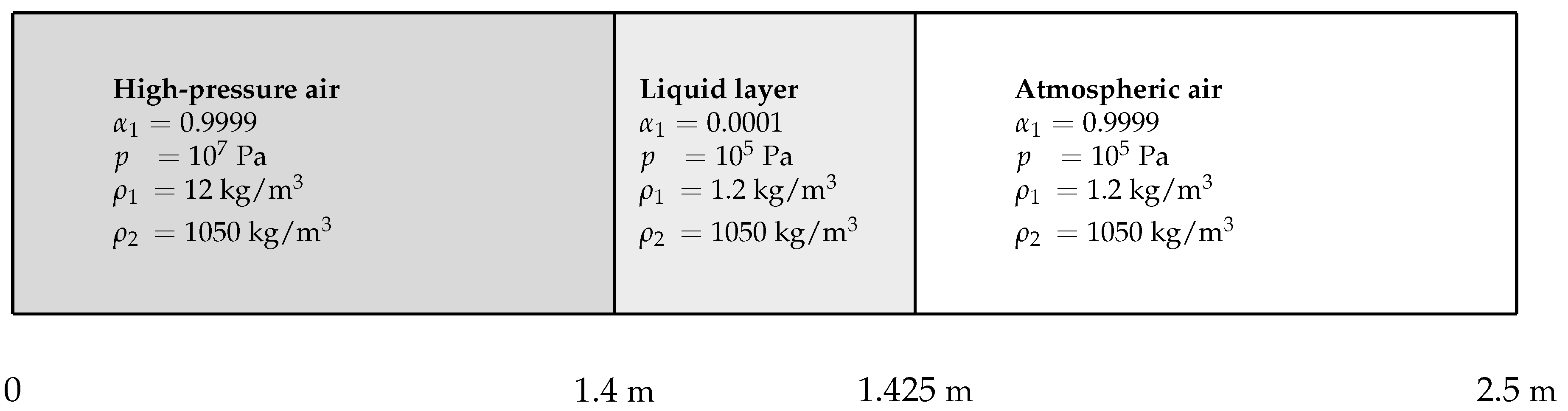
Comparison between the conventional method, considering a single droplet radius in a control volume, and the present method accounting for the polydisperse effects is now addressed. The test case consists of a 1D simplification of the explosion situation depicted in Figure 1. A layer of either monodiperse or polydisperse water droplets is initially present in the 1D domain and is surrounded by air on both sides. Material interfaces are then initially present. On the left of the liquid layer, air is initially at an elevated pressure, and represents initial explosion conditions. On the right, air is at atmospheric conditions. As time goes on, the present initial explosion conditions yield two-phase suspensions. Both material interfaces and two-phase suspensions are then present in this numerical test. The present test case is depicted in Figure 5.

A fractional step method is used. Computation of the source terms of (1) is decoupled from transport and wave propagation. The hyperbolic step, i.e., the resolution of the two-phase flow equation system without pressure and velocity relaxation source terms, is addressed with the first-order Godunov (1959) scheme [47] including non-conservative terms (Saurel and Abgrall, 1999 [38]). Obviously, higher-order methods may be used but add unnecessary complexity. See for example the second-order MUSCL-type method including non-conservative terms presented in Chiapolino et al. (2017) [48] in a similar two-phase context. The first-order method is then preferred as the analysis is free of extra ingredients such as flux limiters and gradient computation. The numerical scheme involves resolution of the Riemann problem and is stable under the conventional CFL condition. In the following, $\mathrm{CFL}=0.8$ for all test cases. The Riemann problem is solved with the help of the HLLC-type solver of Furfaro and Saurel (2015) [49]. Stiff pressure relaxation is considered according to the method provided in Le Métayer et al. (2013) [40]. Coefficient $\mu$, present in the right-hand side of Equation system (1), is then considered very large $\left(\mu \to \infty \right)$.

For both methods, the viscous drag is treated as a velocity source term and is computed with the help of Equations (9) and (12) reminded hereafter,

$$N_2{F}_{1\to 2}=\lambda \left(u_1-u_2\right)\mathrm{with}\lambda =\left(\frac{1}{8}{C}_d{\rho }_1|u_2-u_1|\right)\times A_I.$$

(44)

Turbulent effects are summarized through the $C_d$ coefficient, that is computed with the help of the Naumann and Schiller (1935) [41] correlation (6) and particle Reynolds number (4). Those are recalled hereafter,

$$C_d=\left\{\begin{array}{c}\begin{array}{ccc}\frac{24}{R{e}_2}\left(1+0.15R{e}_p^{0.687}\right)\hfill & \hfill & \mathrm{if}R{e}_2<800,\hfill \\ 0.438\hfill & \hfill & \mathrm{otherwise},\hfill \end{array}\hfill \end{array}\right.R{e}_2=\frac{2R_2{\rho }_1|u_2-u_1|}{{\mu }_1}.$$

(45)

A particle radius $R_2$ is then needed. The very purpose of the present computations is to highlight the effects of the polydisperse character of the liquid cloud on the specific interfacial area $A_I$ only. Consequently, the $R_2$ radius involved in the computation of the drag coefficient $C_d$ is determined with the help of Equation (7) for both methods,

$$R_2=\sqrt[3]{\frac{{\alpha }_2}{\frac{4}{3}\pi N_2}}.$$

(46)

Finally, the specific interfacial area $A_I$ is computed both through its monodisperse simplified formulation (10) and the proposed relation (30) accounting for the polydisperse character of the liquid cloud. As the Gamma (32) and Inverse Gamma (33) PDFs are considered in the present work, the corresponding equations reduce to Equation (38). Those relations are recalled hereafter,

$$A_I=\left\{\begin{array}{ccc}4\pi R_2^2{N}_2,\hfill & \hfill & \mathrm{Monodisperse},\hfill \\ 4\pi N_2(\kappa +1)\kappa {\left(\frac{4\pi N_2}{3{\alpha }_2}(\kappa +2)(\kappa +1)\kappa \right)}^{-\frac{2}{3}},\hfill & & \mathrm{Polydisperse}\mathrm{Gamma},\hfill \\ \frac{4\pi N_2}{(\kappa -2)(\kappa -1)}{\left(\frac{3{\alpha }_2}{4\pi N_2}(\kappa -3)(\kappa -2)(\kappa -1)\right)}^{\frac{2}{3}},\hfill & & \mathrm{Polydisperse}\mathrm{Inverse}\mathrm{Gamma}.\end{array}\right.$$

(47)

Recall that ${\alpha }_2$ and $N_2$ are provided by the balance equations of (1). For the sake of clarity, only the Inverse Gamma PDF is used in the following. For both phases, the Stiffened-Gas equation of state (Le Métayer et al., 2004 [50]) is considered,

$$p_k\left({\rho }_k,e_k\right)=\left({\gamma }_k-1\right){\rho }_k{e}_k-{\gamma }_k{p}_{\infty ,k},$$

(48)

with ${\gamma }_k$ the ratio of heat capacities $\left({\gamma }_k=C_{p,k}/C_{v,k}\right)$ and $p_{\infty ,k}$ a constant related to the attractive effects of phase k. The dynamic viscosity of the gas phase is ${\mu }_1=$ 1.8 × 10⁻⁵ Pa . s. The various equation-of-state parameters are provided in

Table 2. Stiffened-Gas coefficients for air and liquid water [32].

Coefficients	$\mathit{\gamma }$	${\mathit{P}}_{\mathit{\infty }}\left(\mathbf{Pa}\right)$
Gas Phase	$1.4$	0
Liquid Phase	$4.4$	$6\times {10}^8$

.

5.1. Monodisperse

First, results provided by the monodisperse simplification are presented. In the following, three initial particle radii are considered, namely $R_2^{t=0}=3$ $\mathsf{\mu }$m, $R_2^{t=0}=30$ $\mathsf{\mu }$m and $R_2^{t=0}=300$ $\mathsf{\mu }$m. Those three radii lead to three initial specific numbers of particle $N_2^{t=0}$ through Equation (7): $N_2^{t=0}=\left(3{\alpha }_2\right)/\left(4\pi R_2^{3,t=0}\right)$. A single size of particle is considered in a control volume. However, the radius $R_2$ evolves with time through Equation (46) as the liquid volume fraction ${\alpha }_2$ and the specific number of particle $N_2$ are provided by the balance Equation (1). 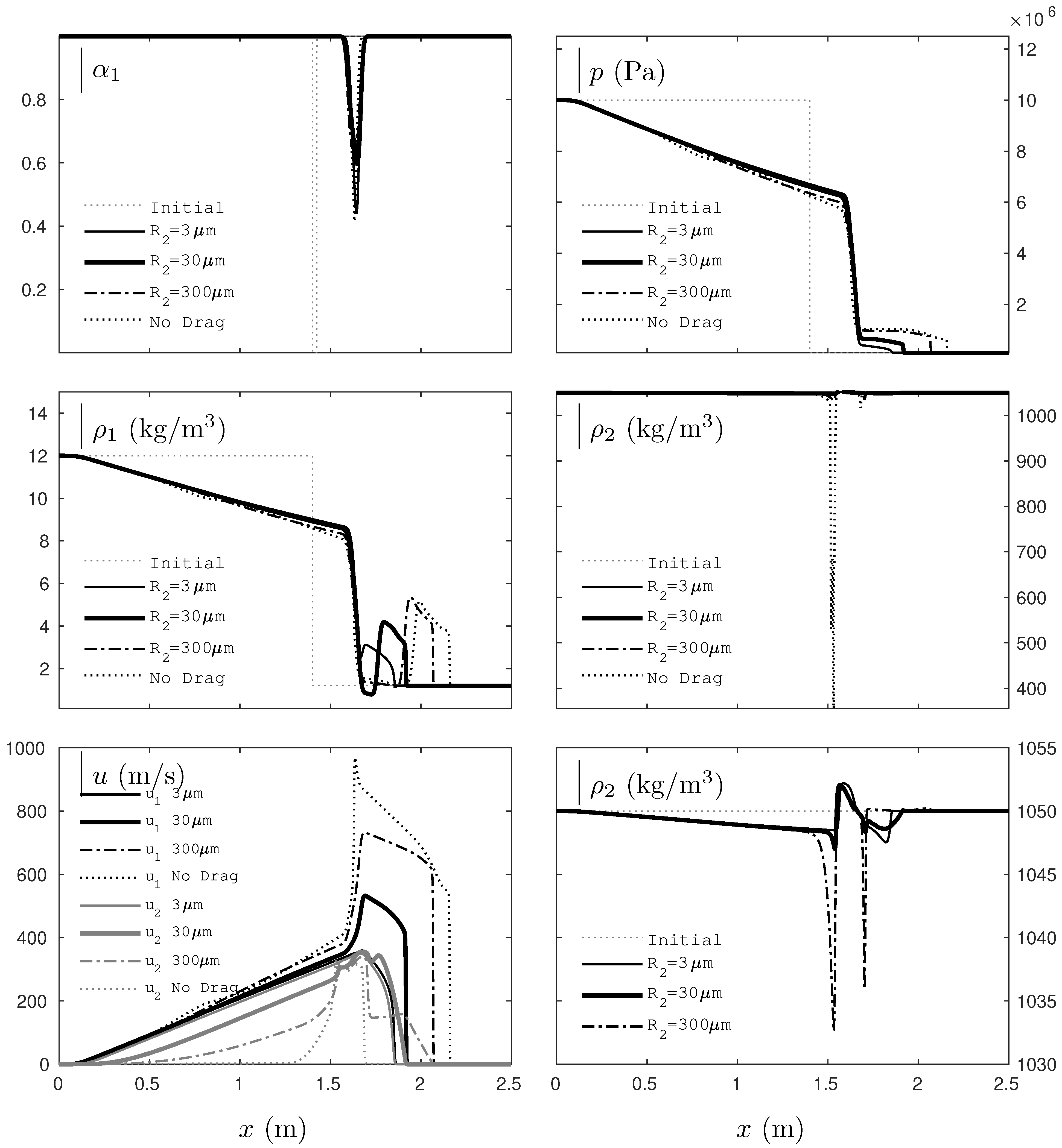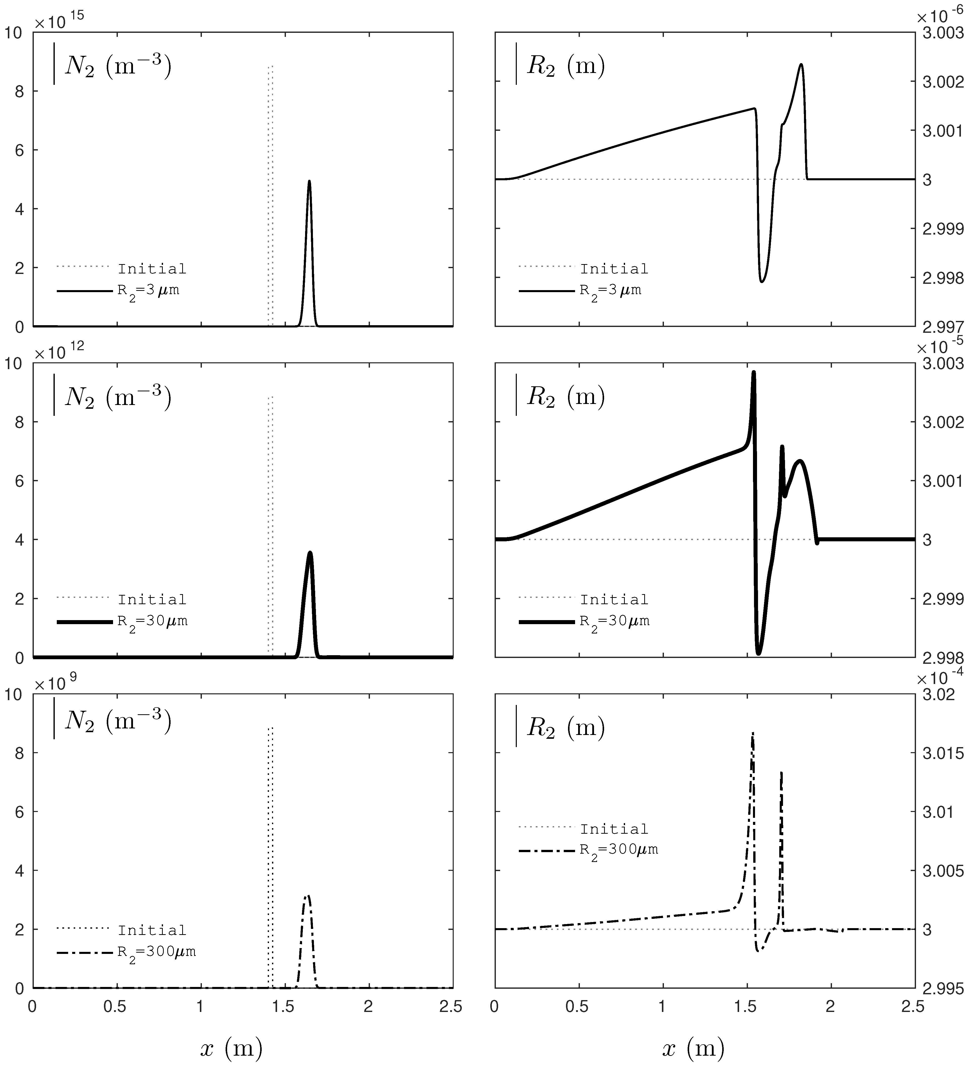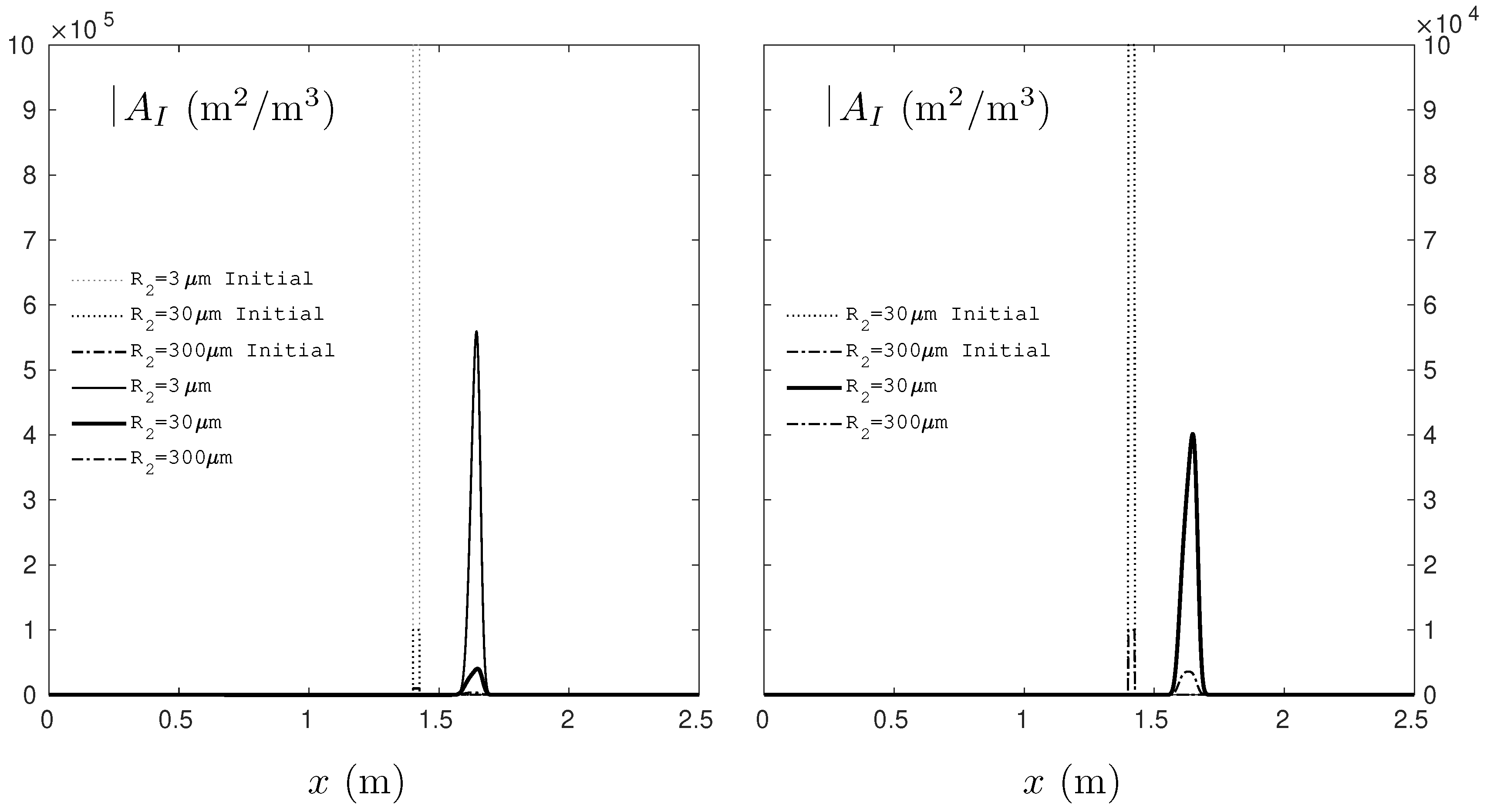The corresponding results are given in Figure 6, Figure 7 and Figure 8. Computation in the absence of viscous drag force is also considered for the sake of comparison.

Results provided by Figure 6 indicate that the larger the liquid particles are, the faster the incident shock wave goes. Indeed, the initial amount of liquid is the same for all computations: ${\alpha }_2^{t=0}=0.9999$ in the liquid layer. The larger the droplets are in a control volume, the smaller their number $N_2$ is as verified in Figure 7. Consequently, the interfacial $A_I$ in this very same control volume is lesser when the droplets are large as seen in Figure 8.

The specific interfacial area $A_I$ describes the available interaction surface between the gas and the liquid phases in a control volume and affects the viscous drag force (Equation (44)). When the interfacial area is small, the viscous interactions are weak between the two phases and the shock wave initiated by the high-pressure air travels faster. In that event, the speed of the air $u_1$ and of speed of the liquid droplets $u_2$ are quite different as seen in Figure 6. The largest difference is found in the absence of viscous drag where consequently no interaction (other than the one described by the non-conservative terms) is present. The incident shock wave is also the fastest in these circumstances. Oppositely, when the specific interfacial area is large as a result of the smallest particle radius ($R_2^{t=0}=3$ $\mathsf{\mu }$m), the viscous interactions between the two phases are strong and the incident shock wave is the slowest. The liquid droplets being small, those are easily dragged by the carrier air phase. Indeed, Figure 6 shows that the speed of the droplets $u_2$ is quasi identical to the speed $u_1$ of the carrier phase.

The size $R_2$ of the liquid droplets clearly impacts the two-phase flow solution through the specific interfacial area $A_I$ and consequently through the viscous interactions between the gas and the liquid phases. The previous computations are simplified in the sense that a single size of particles is considered in a control volume. In the following, the polydisperse aspect of the liquid droplets is accounted for according to the method presented earlier. All corresponding results are plotted against those provided by the monodisperse simplification with an initial radius of $R_2^{t=0}=30$ $\mathsf{\mu }$m.

5.2. Polydisperse

The initialization of the two-phase flow conditions is performed according to the method presented in Section 4.2.1. As previously with the monodisperse computations, the initial volume fraction ${\alpha }_2^{t=0}$ of the liquid phase is considered as an input data, as it is usually the case in two-phase flow computations. The initial mean radius, i.e., ${\overline{R_2}}^{t=0}$ for the polydisperse computation or $R_2^{t=0}$ for the monodisperse computation, is also known either as an input data point or with the help of Equation (39) ensuring a common initial specific interfacial area $A_{I,\mathrm{mono}.}^{t=0}=A_{I,\mathrm{poly}.}^{t=0}$ as detailed in Appendix C. Indeed, for a proper comparison of the two computations, the following test cases consider either a common initial specific interfacial area $A_{I,\mathrm{mono}.}^{t=0}=A_{I,\mathrm{poly}.}^{t=0}$ or a common mean radius ${\overline{R_2}}^{t=0}=R_2^{t=0}$ between the two computations. 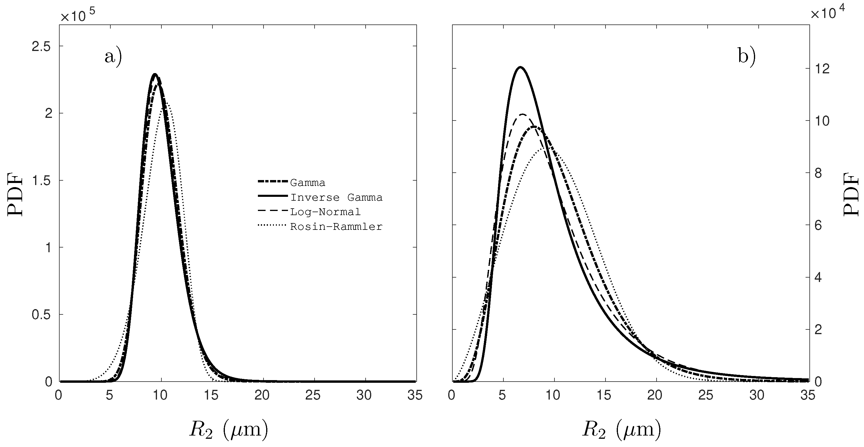For the polydisperse computations the Inverse Gamma probability density function is considered with various $\kappa$ parameters. 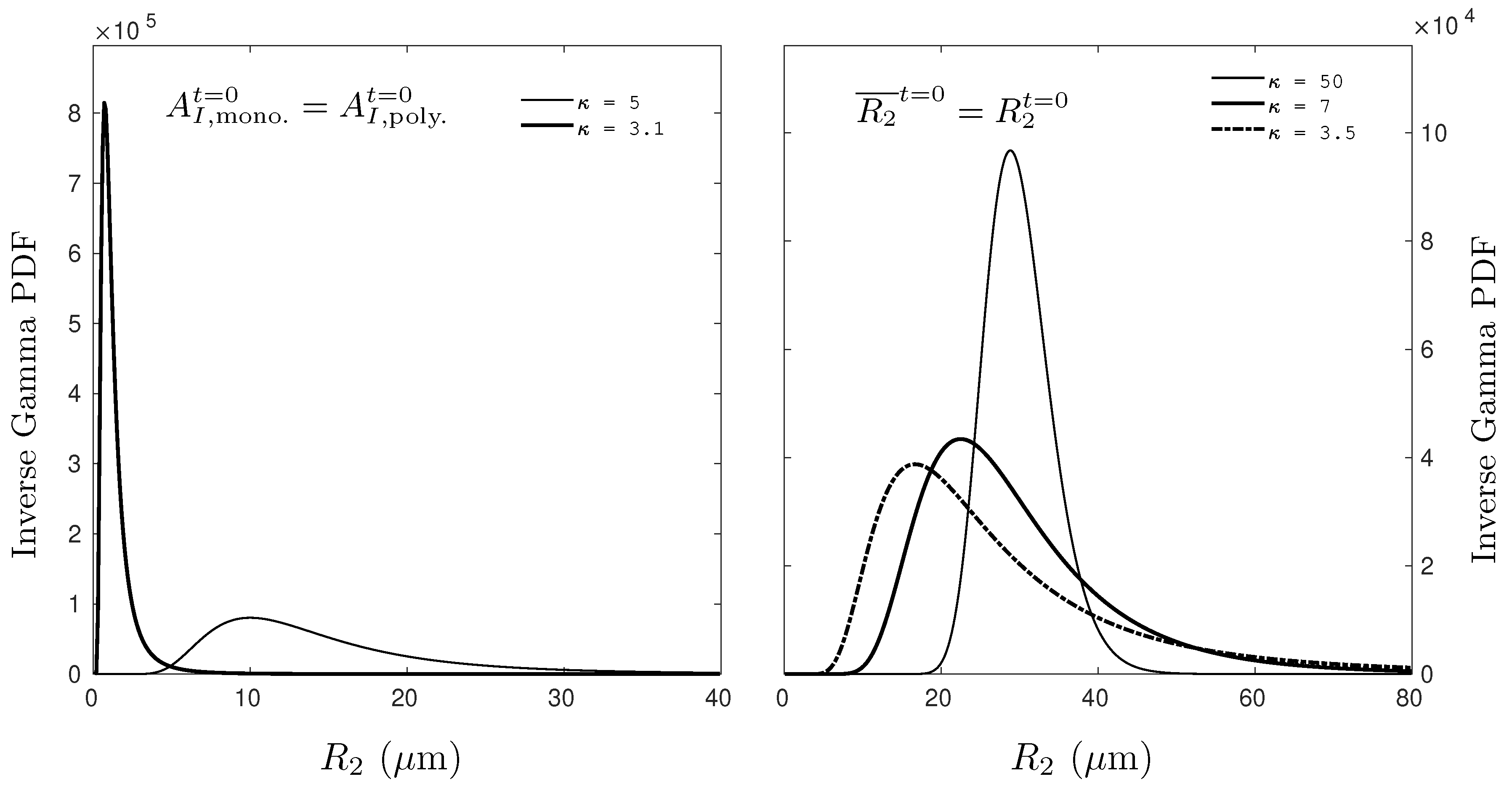The resulting initial droplet distributions are depicted in Figure 9 for the two events, i.e., common initial interfacial area or common initial mean radius between the monodisperse and polydisperse computations.

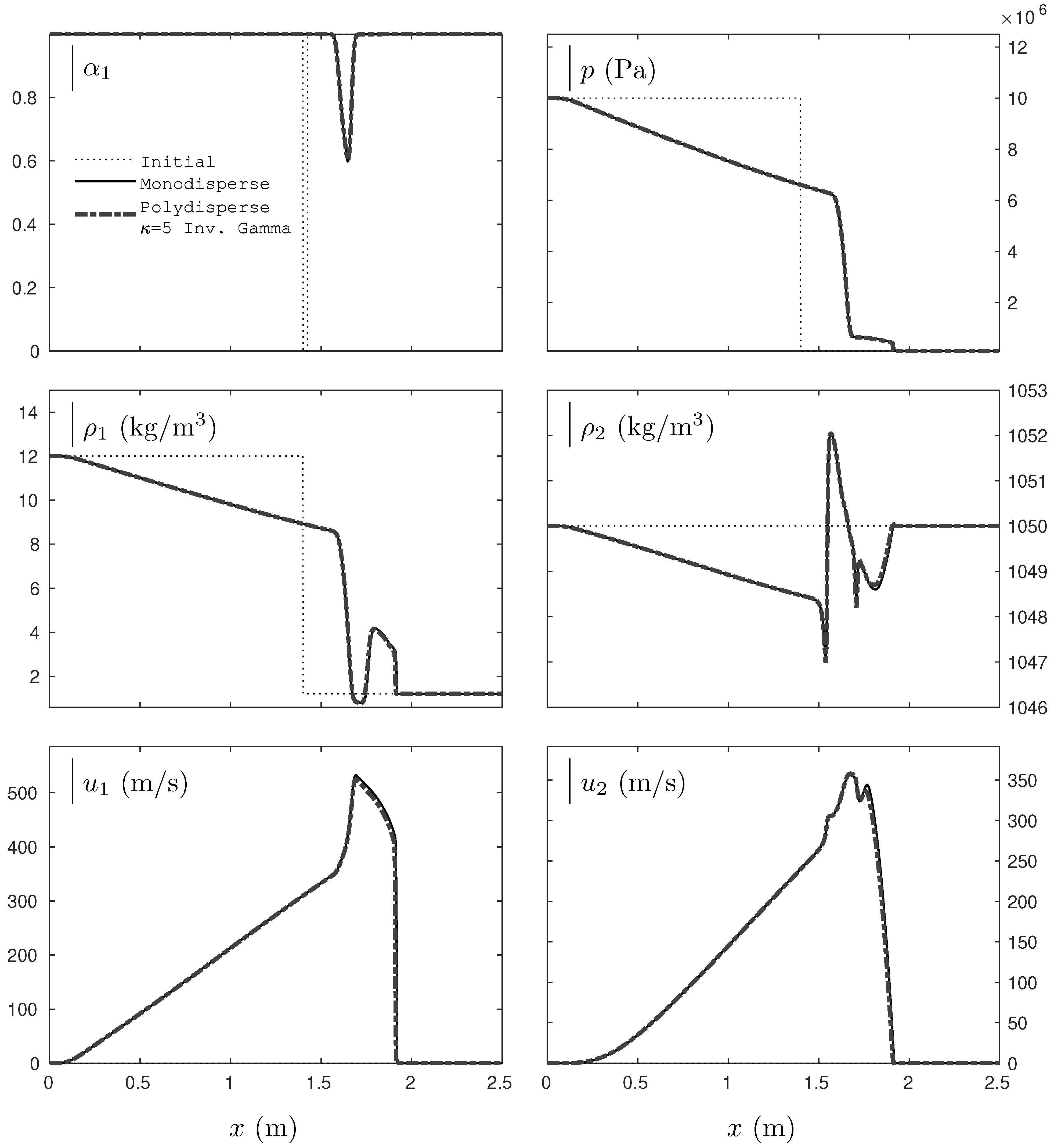
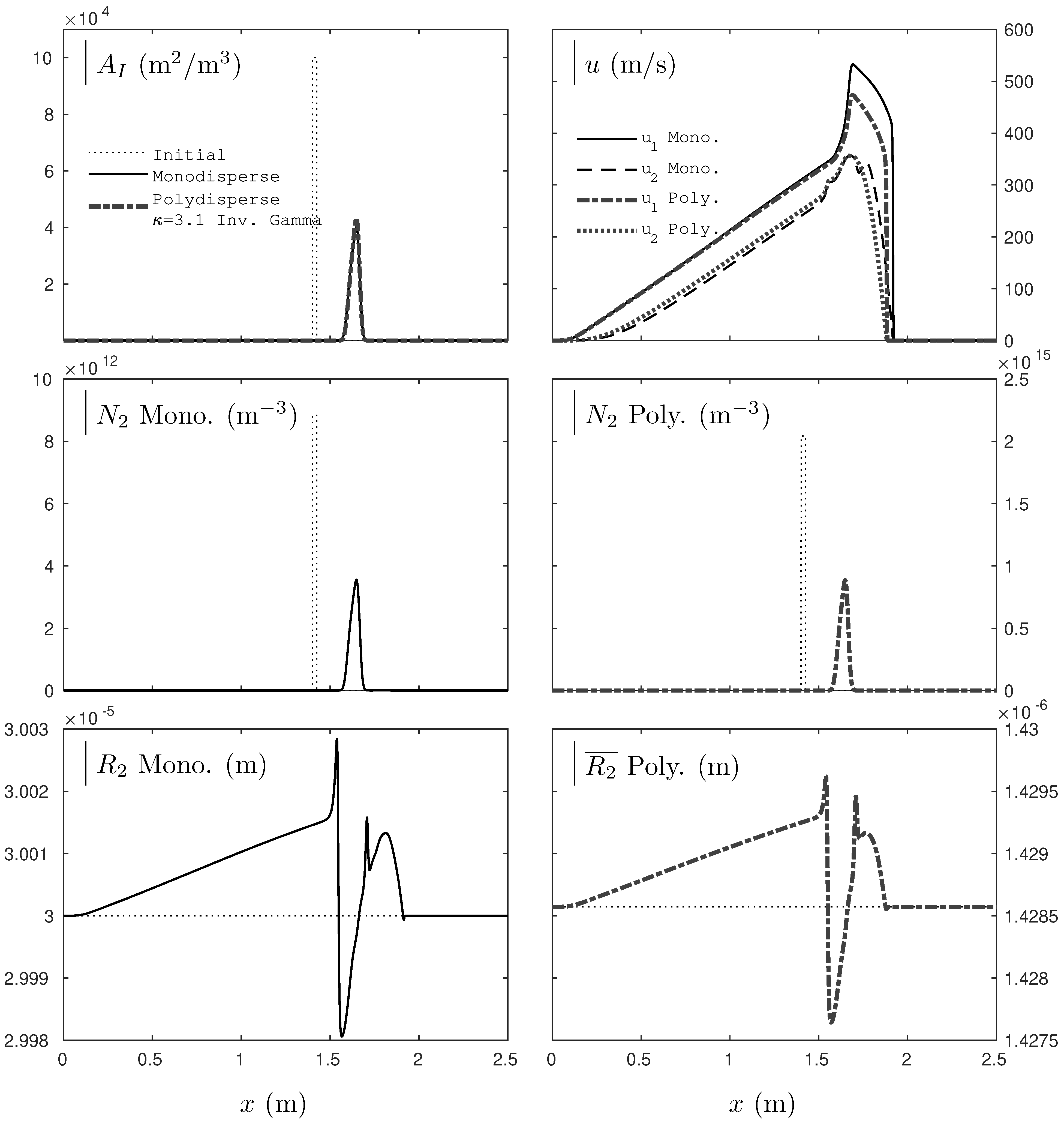
5.2.1. Common Initial Interfacial Area $A_I^{t=0}$ between the Polydisperse and Monodisperse Computations

The analysis begins with the first situation, i.e., the initial specific interfacial area is common between the two computations $A_{I,\mathrm{mono}.}^{t=0}=A_{I,\mathrm{poly}.}^{t=0}$. Examining the evolution of the polydisperse solution when initialized with the same initial specific interfacial area as the one of the monodisperse situation is important. Indeed, as seen previously with the monodisperse computations, $A_I$ plays a major role in the viscous interactions between the phases. The following results show how the polydisperse solution departs from the monodisperse simplification and show the impact of the polydisperse character of the liquid droplets on their mean radius $\overline{R_2}$ and volume fraction ${\alpha }_2$.

The initial mean radius of the monodisperse computation is $R_2^{t=0}=30$ $\mathsf{\mu }$m. Two $\kappa$ parameters are considered, $\kappa =5$ and $\kappa =3.1$. As seen in Figure 9 those two parameters lead to very different initial size distributions. Yet, those two distributions yield the same initial specific interfacial area $A_I^{t=0}$ that corresponds to one of the monodisperse computation. When $\kappa =3.1$, the PDF indicates a high probability to obtain droplets of radii $R_2\simeq 1$ $\mathsf{\mu }$m. However, such a low value appears quite close to the minimum physical radius $R_{\min }$ estimated with the help of the critical Weber number, and may consequently be problematic as regards to the physical representation of liquid droplets. The present size distribution mathematically provides $A_{I,\mathrm{mono}.}^{t=0}=A_{I,\mathrm{poly}.}^{t=0}$ but appears fictitious. We will come back to this point a bit further. 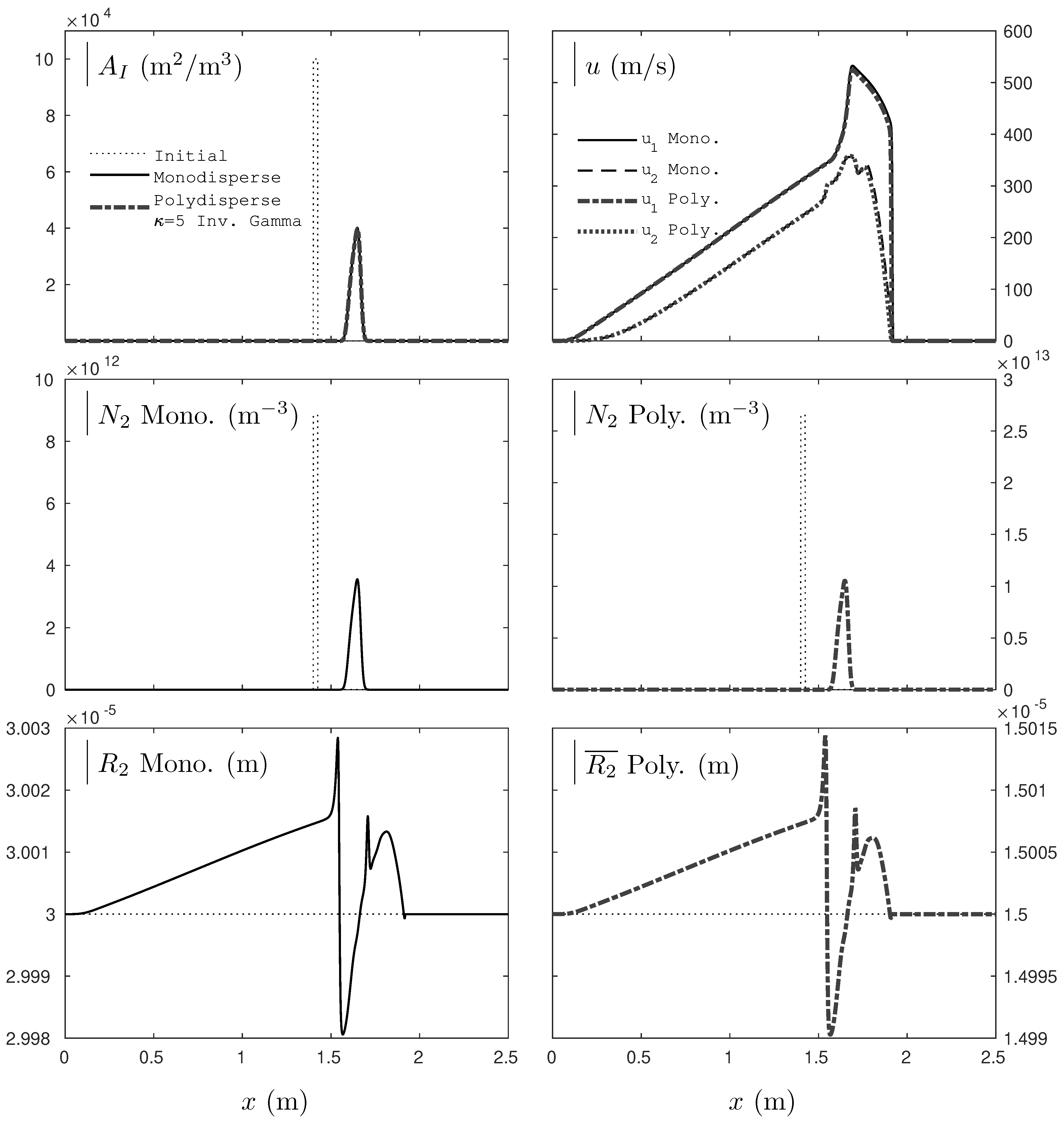Beforehand, the monodiperse results and the polydisperse results obtained with $\kappa =5$ are compared. The corresponding results are presented in Figure 10 and Figure 11.

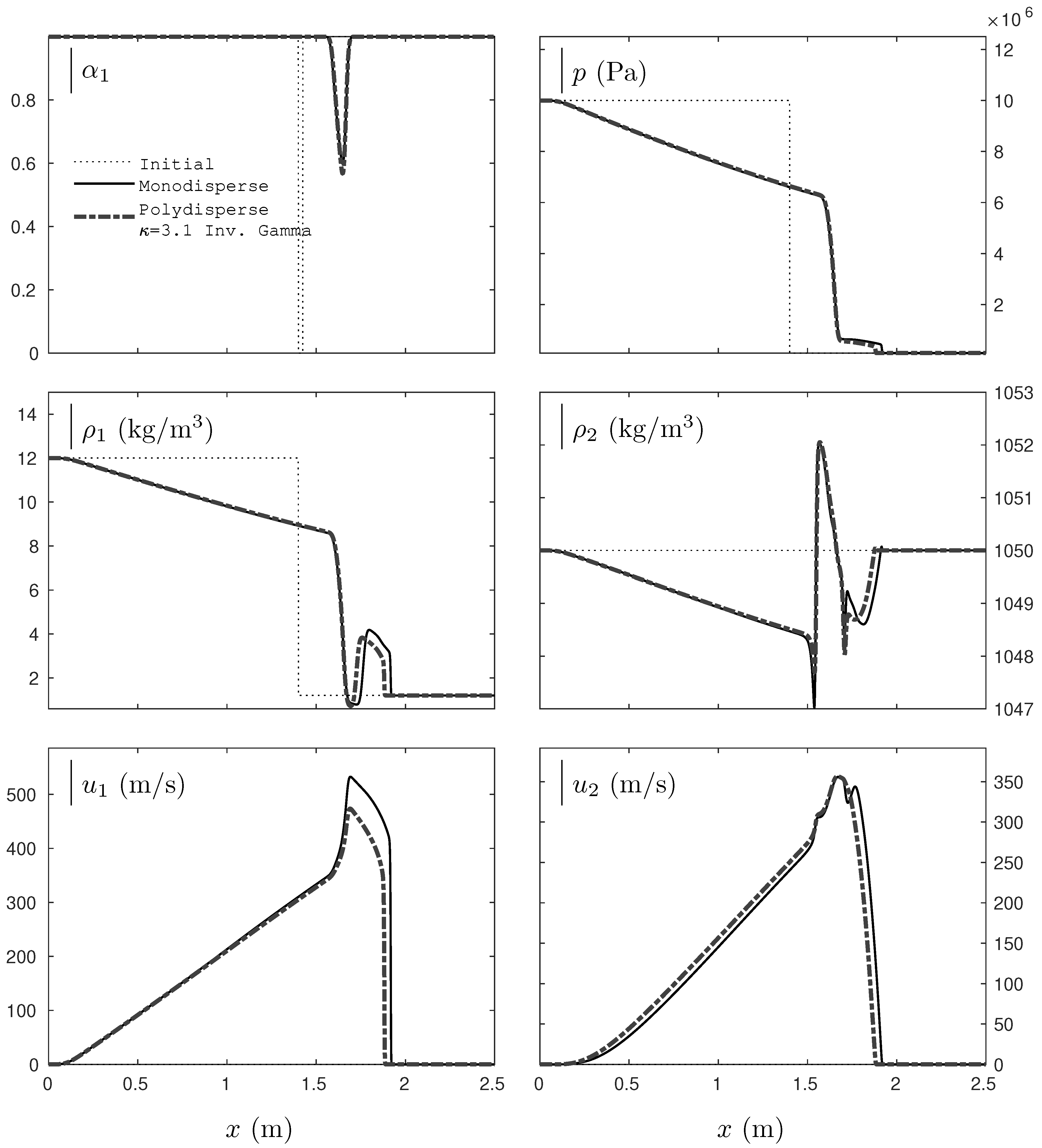
In the present conditions, when ${\kappa }_{\mathrm{Gamma}}^{\mathrm{Inverse}}\ge 5$, the different flow variables of the monodisperse and polydisperse computations are quasi merged, except for the mean radius $\overline{R_2}$ and the specific number $N_2$ of the liquid droplets. However the resulting specific interfacial areas $A_I$ are very close. It then appears that with the present conditions, the polydisperse effects are correctly reproduced by the monodisperse simplification. The test is now repeated with a lower value of the $\kappa$ parameter. This last one is now set to $\kappa =3.1$ and is close to its admissible lower limit. Figure 12 and Figure 13 present the corresponding results.

The $\kappa$ parameter being close to its lower limit, the impact of the PDF, taking into account the polydisperse effects, is now clearly seen on the various flow variables. Indeed, the present results show the impact of the particle size on the specific interfacial area $A_I$ and consequently on the flow variables $\left(\alpha ,p,\rho ,u\right)$ through the viscous interactions between the carrier gas phase and the dispersed liquid phase. Nevertheless, as indicated earlier by Figure 9, the mean radius $\overline{R_2}$ of the polydisperse droplets is physically questionable as it tends to the minimum physical radius $R_{\min }\simeq 1$ $\mathsf{\mu }$m estimated with the help of the critical Weber number. Those very small particles then appear fictitious. Such an issue is controlled with the second initialization option that is now addressed.

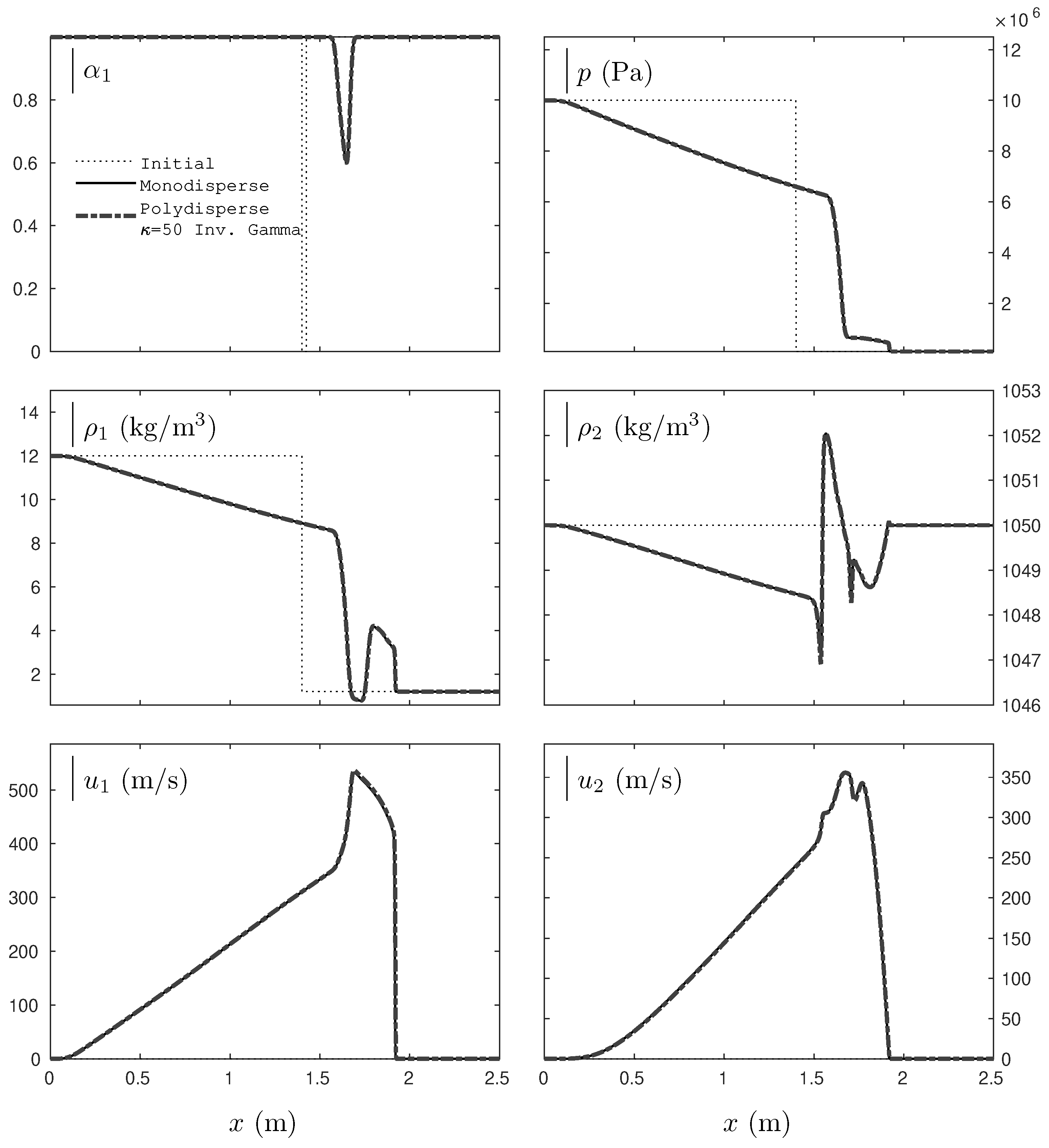
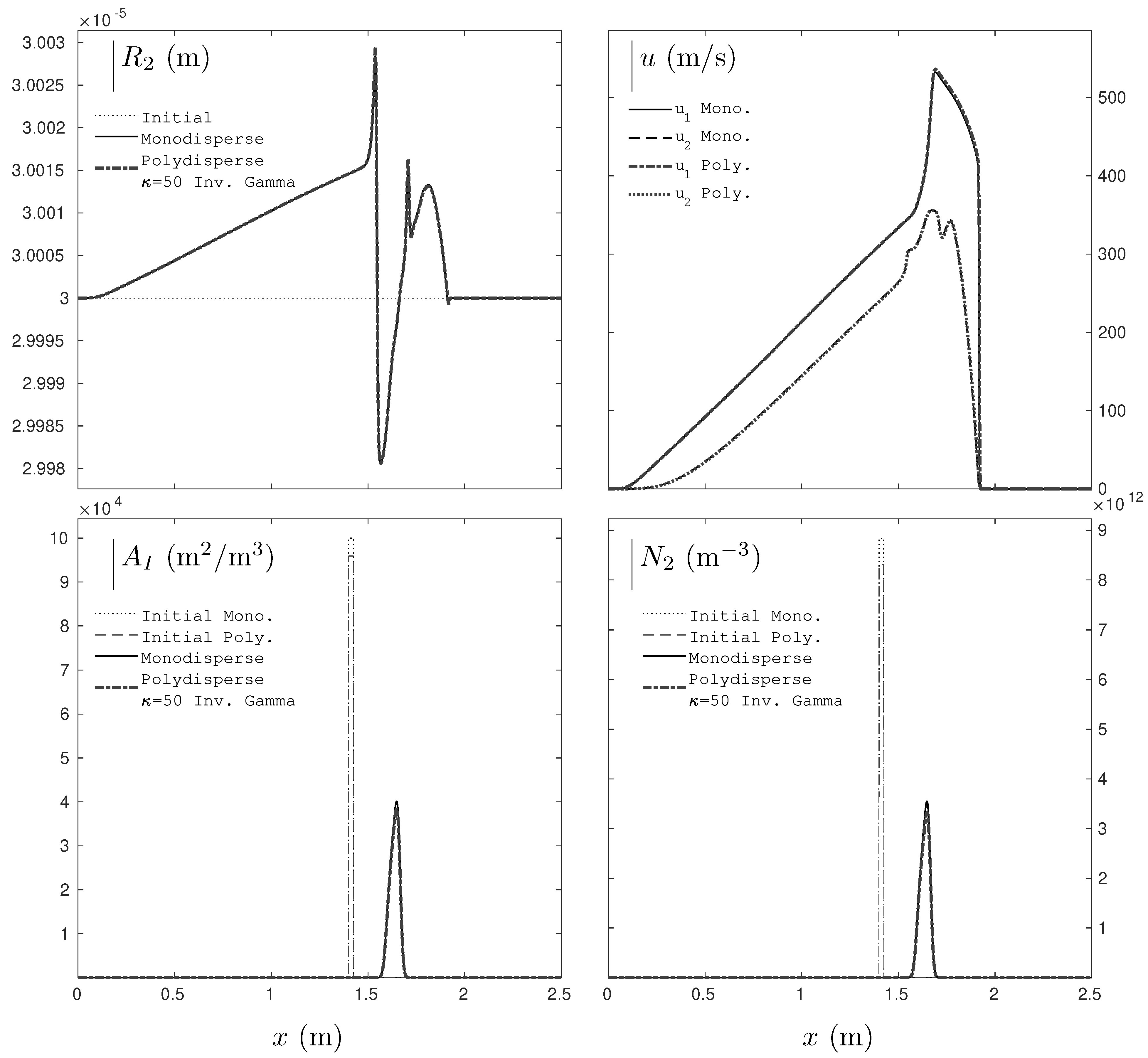
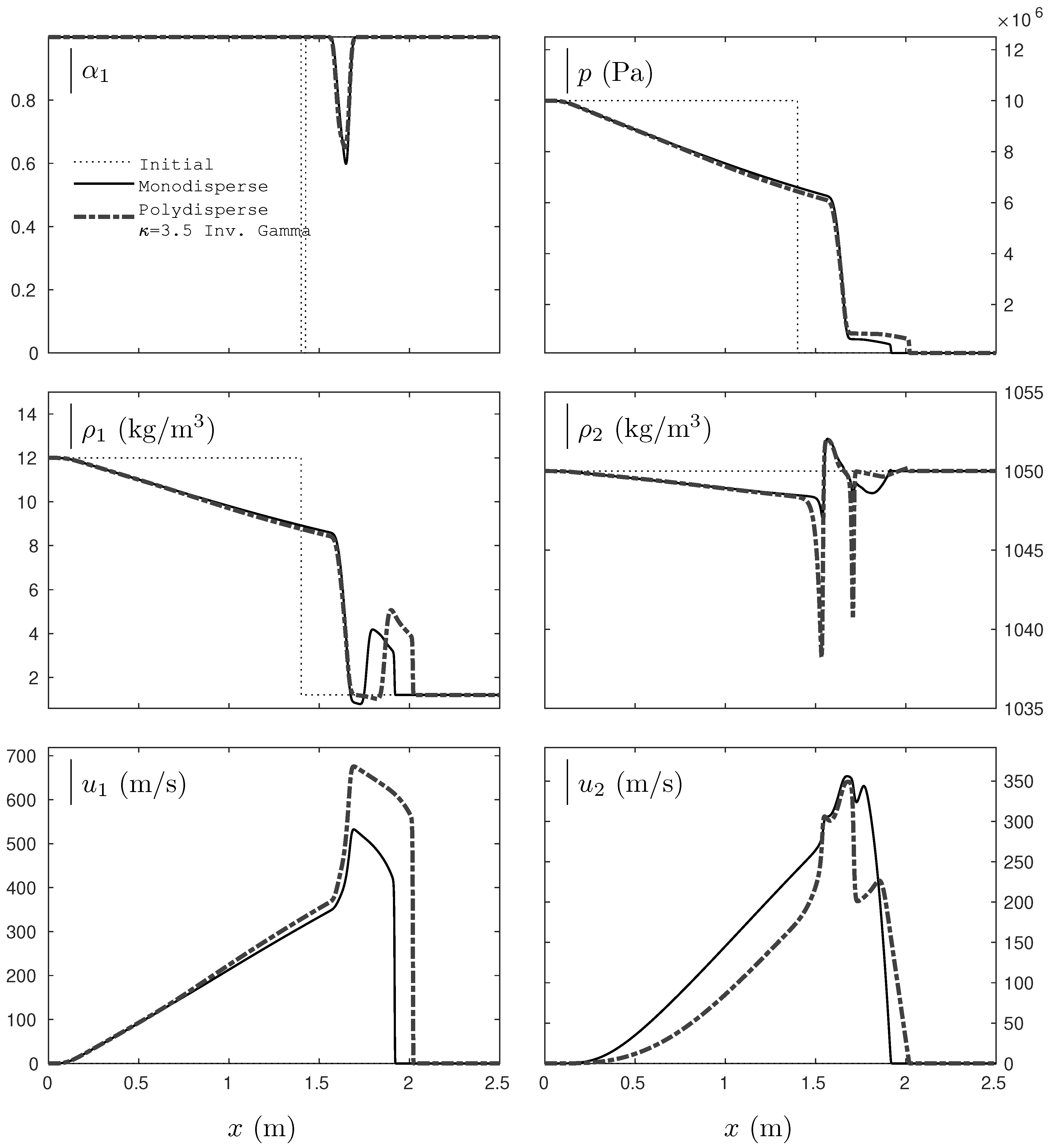
5.2.2. Common Initial Mean Radius ${\overline{R_2}}^{t=0}$ between the Polydisperse and Monodisperse Computations

Unlike the previous results, the initial mean radius ${\overline{R_2}}^{t=0}$ of the polydisperse computation and the initial single radius $R_2^{t=0}$ of the monodisperse computation are now identical. The initial specific interfacial areas are consequently different $A_{I,\mathrm{mono}.}^{t=0}\ne A_{I,\mathrm{poly}.}^{t=0}$, as one is based on a polydisperse distribution of the droplets and the other supposes a single size (Equation (47)). For the following test case, the initial mean radius is set to ${\overline{R_2}}^{t=0}=R_2^{t=0}=30$ $\mathsf{\mu }$m. Figure 14 and Figure 15 compare the results provided by the monodisperse formulation of the specific interfacial area and those provided by the polydisperse relation (Equation (47)). In this last situation, the Inverse Gamma PDF is used with $\kappa =50$.

One more time, the $\kappa$ parameter being quite large, the interfacial area $A_I$ of the polydisperse case is very close to the interfacial area provided by the monodisperse computation, as seen in Figure 15. Consequently, the two solutions are in close agreement as well. The test is now repeated with a lower value: $\kappa =7$. The corresponding results are provided in Figure 16 and Figure 17.

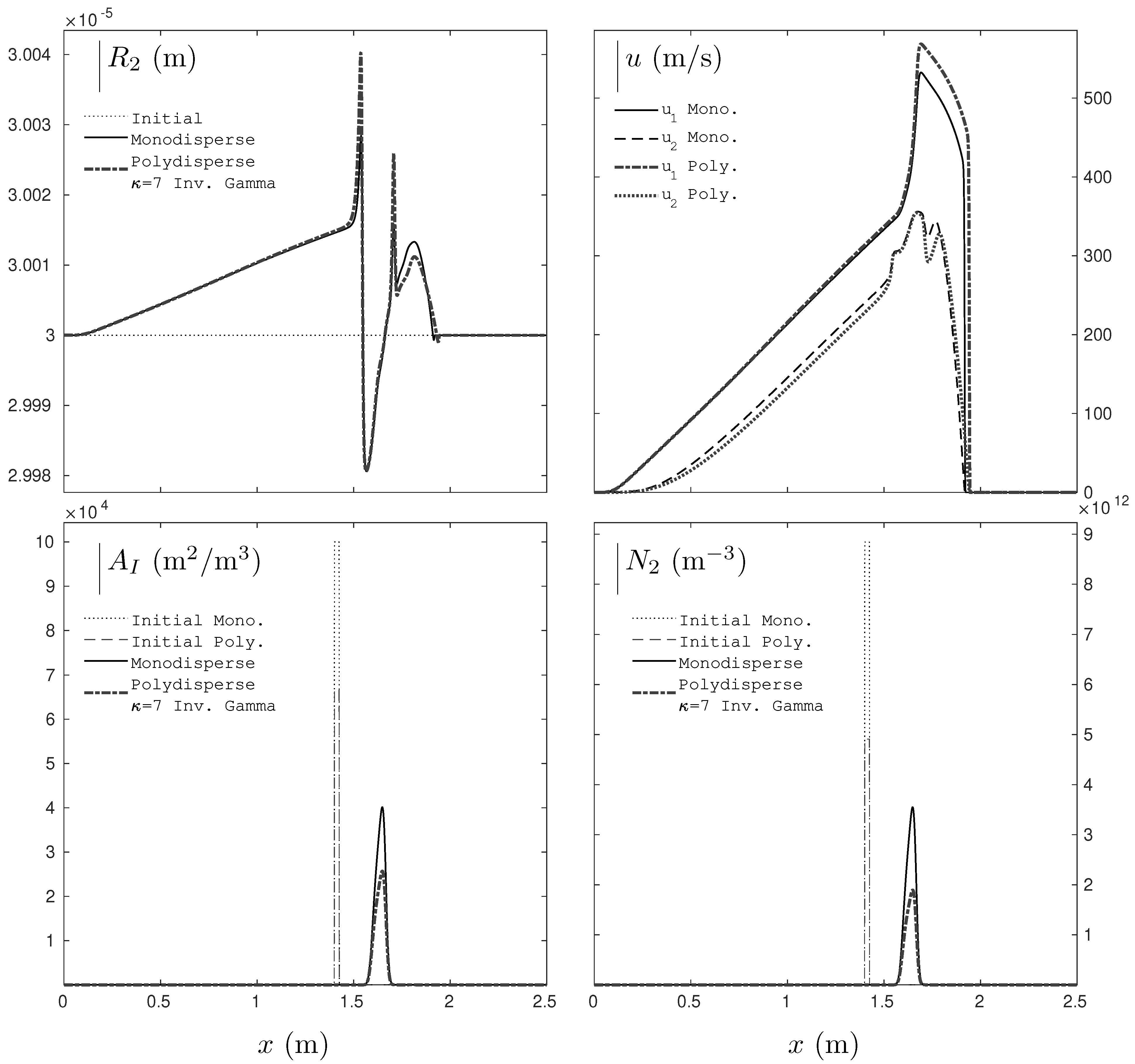
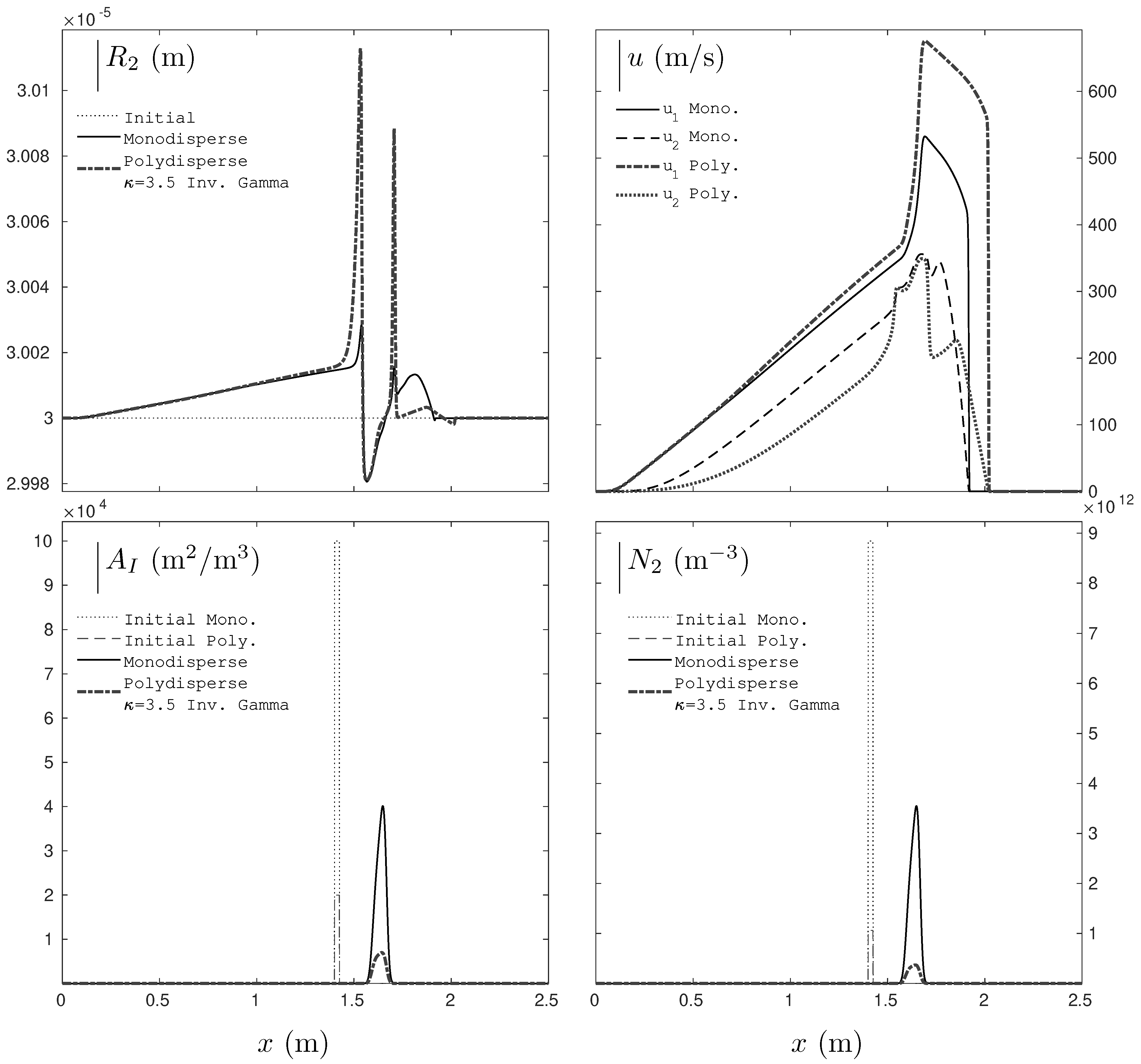
The $\kappa$ parameter being lower, the specific interfacial areas $A_I$ of the two computations are clearly different, as seen in Figure 17. The interfacial area provided by the polydisperse computation is less than the one provided by the monodisperse computation. The two-phase solutions are consequently different. Indeed, the available interaction surface between the gas and liquid phases is lesser and yields consequently a faster shock wave as suggested by the monodiperse analysis provided in Section 5.1. In the following, the $\kappa$ parameter is lowered further, to $\kappa =3.5$. The corresponding results are provided in Figure 18 and Figure 19.

The $\kappa$ parameter is closer to its lower limit ($\kappa =3$). The specific interfacial area $A_I$ provided by the polydisperse computation is significantly less than the one provided by the monodisperse computation as seen in Figure 19. The polydisperse effects consequently affect significantly the shock wave that is much faster due to the lesser available interaction surface between the two phases. The flow variables $\left(\alpha ,\rho ,p,u\right)$ are consequently affected as well. The present results are similar to the one provided by the monodisperse simplification in the event of large particles yielding weak viscous interactions (Figure 6, Figure 7 and Figure 8 of Section 5.1).

The previous results highlight the contribution of the polydisperse effects on the two phase flow, especially on the viscous interactions appearing in the relaxation zone between the gas and liquid phases. Those viscous interactions, and consequently the size of the relaxation zone, are controlled by the specific interfacial area, a key point in combustion and two-phase flow modeling. As seen in Figure 19, the mean radius $\overline{R_2}$ of the polydisperse solution is quite close to the single radius $R_2$ delivered by the simplified monodisperse computation. However, polydisperse droplets have a major impact on the specific interfacial area and consequently on the flow variables.

Two initialization options have been tested. The first one involves an identical initial specific interfacial area $A_{I,\mathrm{mono}.}^{t=0}=A_{I,\mathrm{poly}.}^{t=0}$ for the monodisperse and polydisperse computations. The second involves an identical mean radius of the droplets ${\overline{R_2}}^{t=0}=R_2^{t=0}$. For both cases, the monodisperse and polydisperse solutions are quasi merged when the $\kappa$ parameter is large enough as suggested by the analysis carried out in Section 4.3. For lower $\kappa$ values, clear differences appear. Nevertheless, with the first set of results (identical initial $A_I^{t=0}$) the resulting mean radius ${\overline{R_2}}^{t=0}$ of the polydisperse case may be very low and physically questionable. Yet, the second initialization option (identical initial ${\overline{R_2}}^{t=0}=R_2^{t=0}$) gives control on the present issue and clearly shows the impact of the polydisperse effects on the relaxation zone between the gas and liquid phases.

6. Conclusions

Determination of the specific interfacial area $A_I$ is a key problem in two-phase flow modeling. In many situations the liquid phase is said to be polydisperse as it contains a substantial number of droplets of different sizes, making major effects on the two-phase flow. In the present paper, explosion situations are of particular interest. In such circumstances, material interfaces are present at the early times, as well as two-phase suspensions occurring at later timescales. Both interfacial and disperse flow conditions are then present and the two-phase flow model must be able to deal with both situations.

The specific interfacial area $A_I$ has been reconsidered to account for the polydisperse character of the liquid phase in a simplified way. Computation of $A_I$ relies on a continuous probability distribution. Gamma-like probability density functions have been used in the present work. However, the method may be used with various functions as long as their $m_0$, $m_1$, $m_2$ and $m_3$ moments are available. In the context of Gamma and Inverse Gamma distributions, only the $\kappa$ constant is required as an input data, in addition to the initial mean radius ${\overline{R_2}}^{t=0}$ and initial volume fraction ${\alpha }_2^{t=0}$ that are necessary both for the conventional method and for the proposed method. The $\kappa$ constant controls the shape of the polydisperse distribution and can be adapted to multiple situations. The overall method yields only few code modifications while taking into account the polydisperse aspect of the two-phase flow.

The two-phase equation system of Saurel et al. (2003) [17], variant of Baer and Nunziato’s (BN) model (1986) [16], has been considered in the present work, as it is able to deal with both material interfaces and two-phase suspensions. The impact of the polydisperse character of the liquid phase has been highlighted with the help of a simplified 1D two-phase explosion test. This work can be continued in many directions. Among them are the introduction of fragmentation effects of the liquid droplets, as well as thermal effects and combustion processes. Comparison with experimental results is also part of future works.