Article

Geospatial Wildfire Risk Assessment from Social, Infrastructural and Environmental Perspectives: A Case Study in Queensland Australia

by
Mahyat Shafapourtehrany
Kandilli Observatory and Earthquake Research Institute, Department of Geodesy, Bogazici University, Cengelkoy, Istanbul 34680, Turkey
Submission received: 4 December 2022 / Revised: 4 January 2023 / Accepted: 5 January 2023 / Published: 9 January 2023
(This article belongs to the Special Issue Ensuring Safety against Fires in Overcrowded Urban Areas)

Abstract

:
Although it is hard to predict wildfires, risky areas can be systematically assessed and managed. Some of the factors for decision-making are hazard, vulnerability, and risk maps, which are the end product of wildfire mapping. This study deals with wildfire risk analysis in Queensland, Australia. A review of the previous studies focusing on each aspect has been done and used with wildfire records from 2011 to 2019 in Queensland, Australia, to compile the required input models to detect risky wildfire regions. Machine learning (ML) methods of Decision Tree (DT) and Support Vector Machine (SVM) were used to perform hazard assessment. The reason was to select the most accurate outcomes for the rest of the analysis. Among accuracy assessment techniques, the Area Under Curvature (AUC) method was used to evaluate the hazard maps. Prediction rates of 89.21% and 83.78% were obtained for DT and SVM, respectively. The DT prediction value showed that the DT-hazard map was more accurate than the SVM-hazard map. Vulnerability analysis was implemented by assigning weights to each factor according to the literature. Lastly, in order to create the wildfire risk map, the hazard and vulnerability indices were combined. The risk map showed that particularly dense urbanization regions are under future wildfire risk. To perform preliminary land use planning, this output can be used by local governmental authorities.

1. Introduction

For more than 350 million years, wildfires have been closely associated with our environment and society [1]. Their impacts can be grouped into damage to human lives and health [2], damage to infrastructure such as buildings and transportation [3], and damage to the ecosystem (carbon level and air pollution) [4]. Due to the severe social and ecological damage inflicted by wildfires, the demand for proper management and mitigation plans has grown [5]. Recently, the number of wildfires, especially in California, Australia, and Siberia, has increased [6]. Human activities have resulted in increased atmospheric carbon dioxide levels by around 50% relative to pre-industrial levels, which contributed to about a 1.0 °C increase in global warming [7]. Australia is among countries that are a part of this unequivocal global warming trend. Harris and Lucas [8] investigated variations in Australian fire weather in the period from 1973 to 2017. Their study showed that at most observation stations there were linear increased trends in the Forest Fire Danger Index (FFDI). Research by Bowman, et al. [9] stated that due to climate change the current wildfire condition might get worse. According to their research, an increase of 20% to 50% in the number of days conducive to wildfire events is expected in the future. Consequently, by the mid-21st century (2041–2070), it is expected there will be increases in high fire danger, and the number of days per year of high fire danger is expected to be increased by 35% around the world. In general, during the summer, increases in temperature and decreases in humidity are the main reason for high fire danger days [10]. The Black Summer in Australia [11], which happened between December 2019 and February 2020, was caused by both natural and accidental ignitions. According to the recorded data of 14 January 2020, about 18.6 million hectares were burnt, over 5900 buildings were demolished, and many people were killed [12]. This condition makes Australia one of the most prone areas to wildfire [13].
An interesting study by Moritz, Batllori, Bradstock, Gill, Handmer, Hessburg, Leonard, McCaffrey, Odion and Schoennagel [4] explains how to coexist with wildfire. They believe that social and ecological systems will face serious consequences without a wildfire management plan. As humans, we are responsible for wildfire increase in some regions by changing the natural form of the environment. Therefore, the optimal solution is to learn sustainable coexistence with wildfire [14]. Wildfire, and most its negative impacts, can be controlled and minimized by proper management strategies [15]. Increasing the number of wildfires and their damage has encouraged scientists to assess and develop new wildfire risk systems. Current risk is related to the possibility of loss under current conditions [16]. Although the predicted scenarios are not certain, it is possible to estimate their likelihood [5]. Risk is determined as a function of both hazard and vulnerability [17]. To measure risk in a region, hazard and vulnerability needs to be evaluated. According to Gervasi, et al. [18] hazard is a potentially destructive phenomenon that could cause damage to lives, properties, the economy, and the environment. Regarding vulnerability, this refers to the propensity of people and the environment to be affected by hazardous events [19]. These two factors together provide the risk conditions of a region.
This study aims to evaluate the risky zones in Queensland, Australia is one of the most wildfire-hazardous regions, considering its fire history from 2011 to 2019. Social, environmental and economic factors were considered in assessing the vulnerability in this study. The reliability of each analysis is mainly affected by the data used and the methods applied. A comprehensive literature survey selected all factors related to hazard and vulnerability from previous sources. Wildfire management received considerable benefits from newly discovered and tested analytical tools that support a wide range of wildfire-related factors [20]. There are numerous methods available to perform hazard analysis. Each method has advantages and disadvantages. Some of the well-known methods in wildfire mapping are frequency ratio (FR) [21,22], the analytical hierarchy process (AHP) [23], the analytical network process (ANP) [24,25], logistic regression (LR) [26], evidential belief function (EBF) [27], index of entropy (IoE) [28], and ensemble methods [29].
Machine learning (ML) is a category of algorithms that are often used in natural hazard studies [30,31,32]. These methods are able to recognize data patterns and use them to predict possible future scenarios [33]. Compared to some other methods, ML algorithms are very suitable for dealing with natural hazard mapping such as wildfire [33] mapping. The reason is that in wildfire hazard mapping, many parameters with complex physical properties are involved [34]. ML is capable of handling such an analysis and is able to learn from data and perform assessments without expert rules, meaning that ML can circumvent physics-based simulation limitations [35]. A comprehensive review regarding the application of ML in wildfire mapping has been studied by Jain, Coogan, Subramanian, Crowley, Taylor and Flannigan [33]. Their research cites many references (71) that used various ML algorithms to map wildfire hazard, vulnerability, and risk. Due to the efficiency of the ML and its successful history in wildfire studies, Decision Tree (DT) and Support Vector Machine (SVM) were selected to be used in hazard assessment. The reason for considering two methods was to observe the performance of each and select the best to be used in risk assessment.

2. Study Area

Australian ecosystems, such as deserts and tropical forests, are constantly affected by wildfires [36]. Large regions of savannah in northern Australia have been devastated by intense wildfires [4]. Queensland is Australia’s second-largest state (715,000 square miles) and has been considerably affected by wildfire damages [37]. Regarding population, it is the third largest Australian state with an estimated 5.2 million residents (https://www.abs.gov.au/statistics/people/population/national-state-and-territory-population/latest-release, accessed on 30 June 2022). Therefore, it was selected as an appropriate pilot area to perform wildfire analysis (Figure 1). The study area is located in the northeast of the continent (22.5752° S, 144.0848° E). Population and settlements in Queensland are concentrated along the east coast and in the southeast corner of the state [38]. The climate varies significantly across the state resulting in different climate zones [39]. Queensland has six climate zones: tropical, subtropical, temperate, grassland, equatorial, and desert [40]. Each of these climate zones is characterized by specific temperature and rainfall patterns. Figure 1 represents the study area and wildfire records from 2011 to 2019.
The Queensland government has been providing the fire history in Queensland since 1930 (Figure 2). The fires have been captured from field observations and digitization in a mapping application from reference datasets (e.g., topographic, cadastral data, satellite imageries). As can be seen in the Figure 2, there is an increasing trend in the occurrence of wildfires in this region over history.

3. Methodology

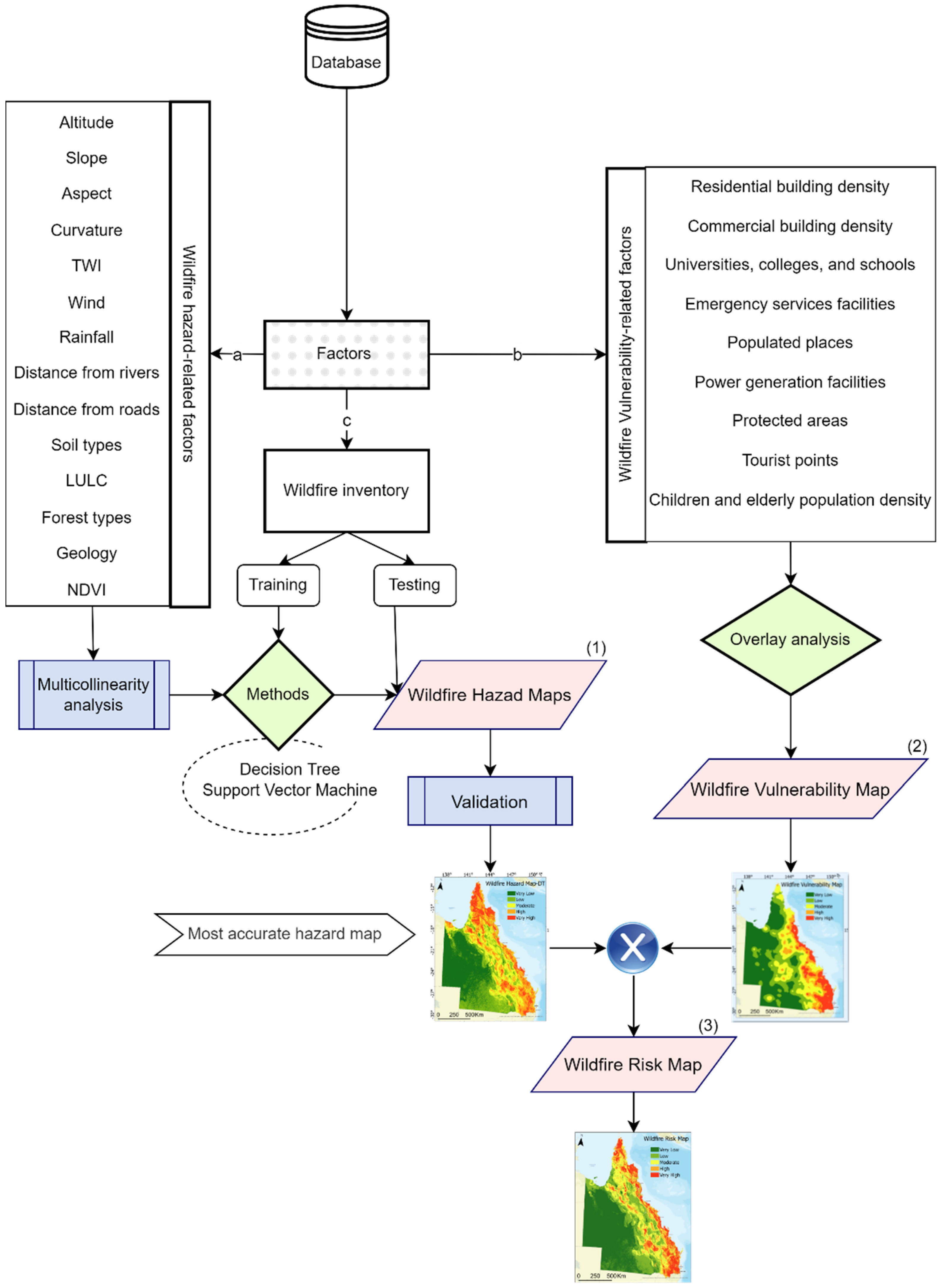
Figure 3 shows the methodology flow chart of the study. The methodology starts by dividing the database into three sets: (a) wildfire hazard-related factors; (b) wildfire vulnerability-related factors, and (c) wildfire inventory. Dataset (a) consists of conditioning factors involved in wildfire hazard analysis, such as altitude, and land use/cover (LULC). Dataset (b), which includes vulnerability-related factors such as population and endangered locations, was used in vulnerability assessment. Dataset (c) is the wildfire records from 2011 to 2019 in Queensland, Australia which was divided into training and testing datasets to be used in hazard modeling and accuracy assessment, respectively. Each dataset is described in its related section. The flowchart also consists of three phases: (1) wildfire hazard analysis using DT and SVM; (2) wildfire vulnerability analysis, and (3) constructing a risk map. The following sections describe the details regarding each phase.

3.1. Data Used

3.1.1. Inventory Dataset

Collecting and managing the datasets are important steps before the generation of natural hazard maps [41]. The GIS database collection starts with creating an inventory map regarding the disasters that occurred in the past [42]. The current study’s inventory dataset represents the wildfire records between 2011 and 2019. Figure 1 shows that wildfires mostly occurred in the far north and the northeast. The inventory dataset was received in polygon format; therefore, a random point selection was applied, and 300 wildfire locations were selected. Following the literature, 70% of the wildfire inventory points were randomly allocated to the training set, and the rest, 30%, were used for testing [43].

3.1.2. Hazard-Related Factors

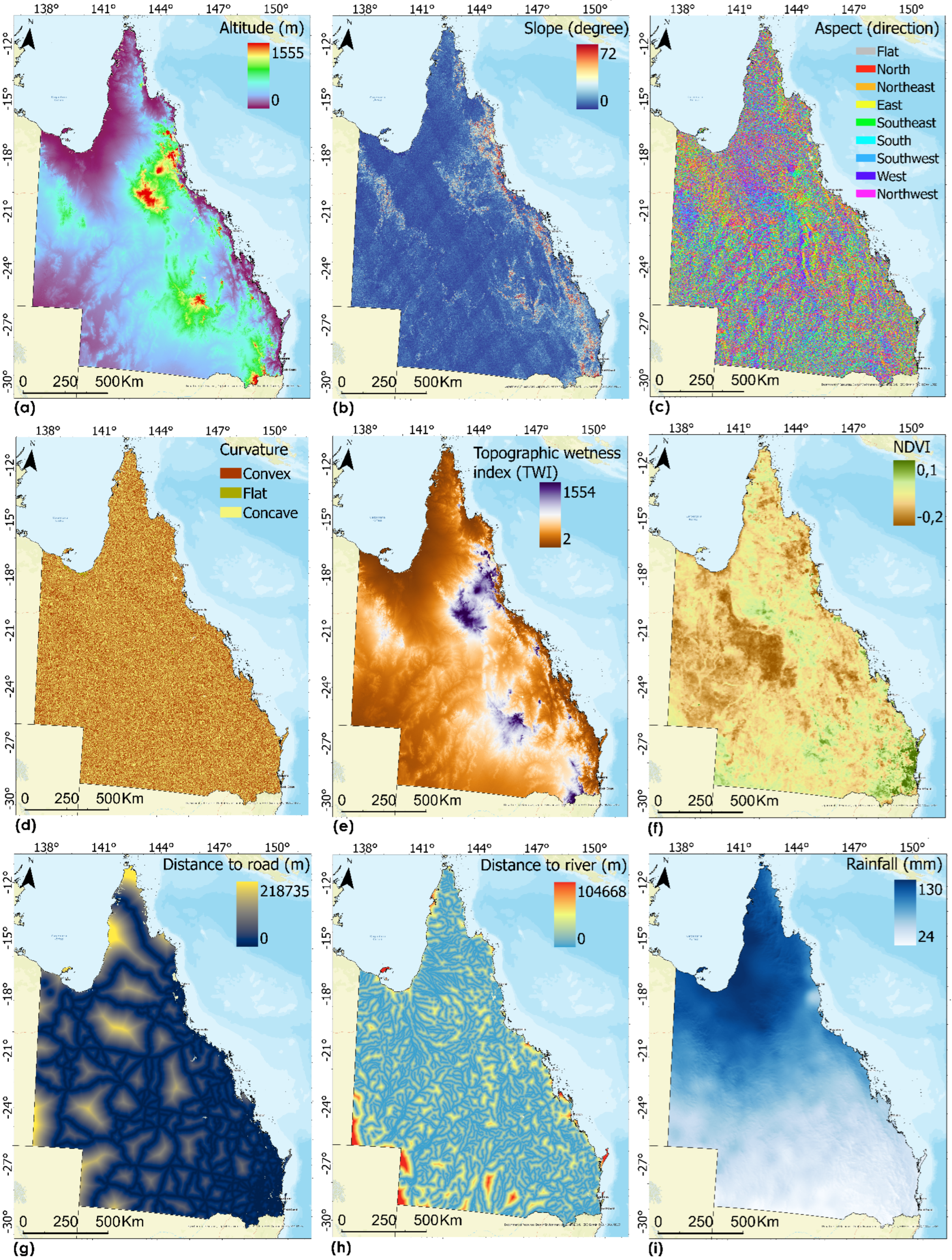
The most effective physical properties that impact wildfire spread are fuel composition, the area’s topography, and weather [33]. Factors influencing wildfire hazards are not limited to the mentioned parameters. A good review of these factors was implemented by Pourtaghi, et al. [44]. According to the literature, there is no fixed dataset creation framework for natural hazard analysis [45]. Therefore, the literature [46], expert knowledge [23], and data availability [45] are the main influential factors for this purpose. The traditional literature-based approach was used in this research to select the primary influencing factors. To apply the wildfire hazard assessment, a spatial database of 14 wildfire hazard-related factors was designed and constructed (Figure 4). Table 1 lists the source for each factor.
In general, the topography of the region is one of the most critical factors in wildfire creation, spread, and extent [47]. Topography itself influences sun exposure, temperature, precipitation, and wind [48]. Three factors of altitude (Figure 4a), slope (Figure 4b), and aspect (Figure 4c) affect the level of solar radiation and fuel moisture content [49]. Fuel preheating spread direction, and slope factors influence the speed of the wildfire. This factor also affects vertical fuel continuity and, therefore, the upward spread of fire [50]. Faster combustion takes place in areas that have sharp slopes as these areas preheat and dry upslope fuels [51]. Vegetation cover is indirectly affected by aspect as it controls the solar radiation received [52]. In the southern hemisphere, north-facing slopes receive higher levels of solar radiation that cause the fuels to dry out more quickly [53]. Therefore, these areas have less vegetation and lighter fuel loads. On the contrary, south-facing slopes have more vegetation and greater fuel quantities. They dry more slowly due to shadows, which cause more severe wildfires.
The morphology of the topography can be measured by curvature values (Figure 4d). Curvature consists of positive values (upwardly convex), zero (flat), and negative values (upwardly concave) [54]. In wildfire studies, the wetness of the ground is essential; therefore, TWI (Figure 4e) was measured, calculated based on Equation (1) [55]:
T W I = l n α t a n β
where the slope angle at the point is tan β and the cumulative up-slope area draining through a point is represented by α.
The NDVI factor (Figure 4f) has been used to measure vegetation cover. It was calculated using Landsat-8 images according to Equation (2):
N D V I = N I R R N I R + R
where NIR and R values are the infrared and red bands, respectively [56].
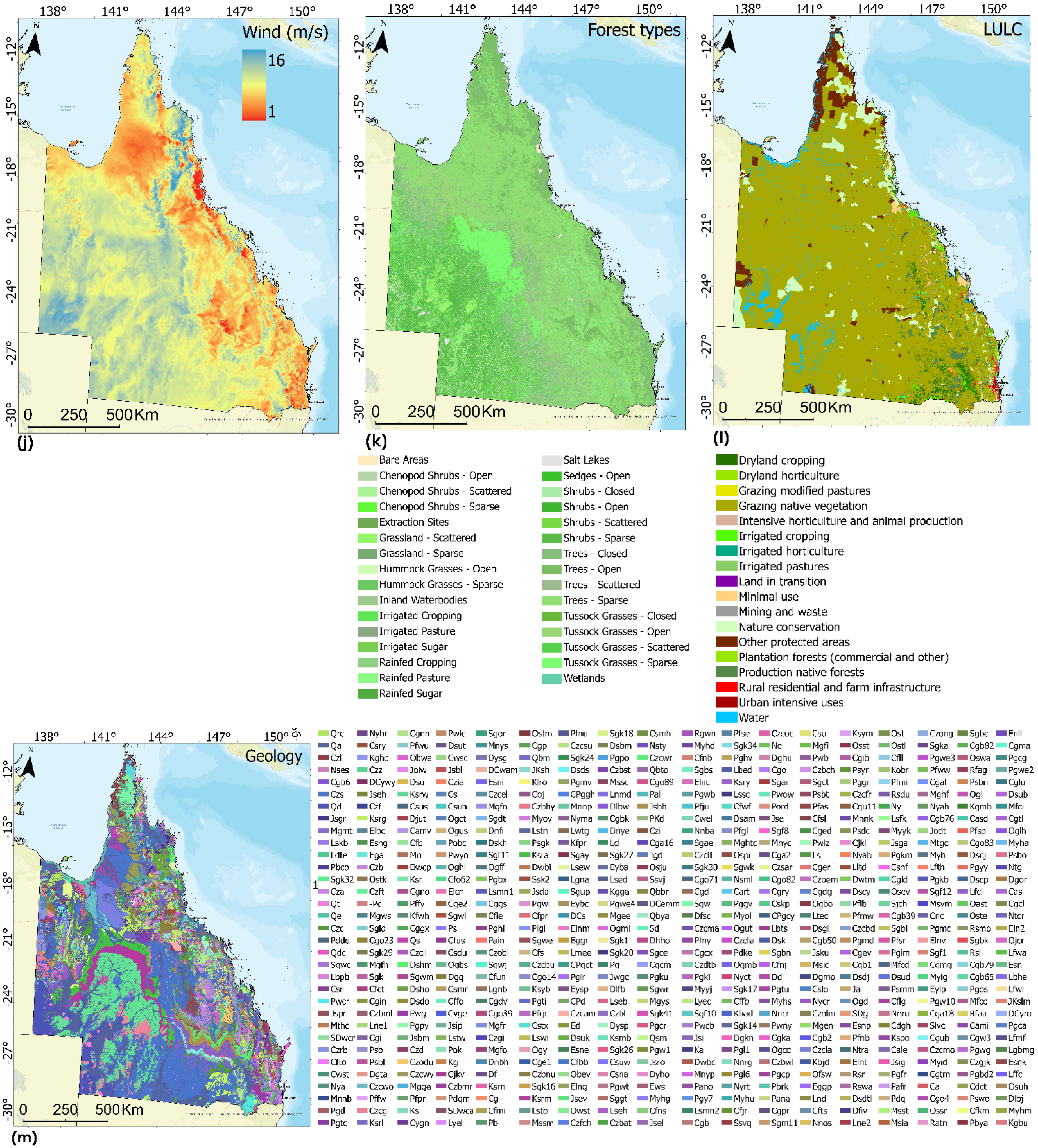
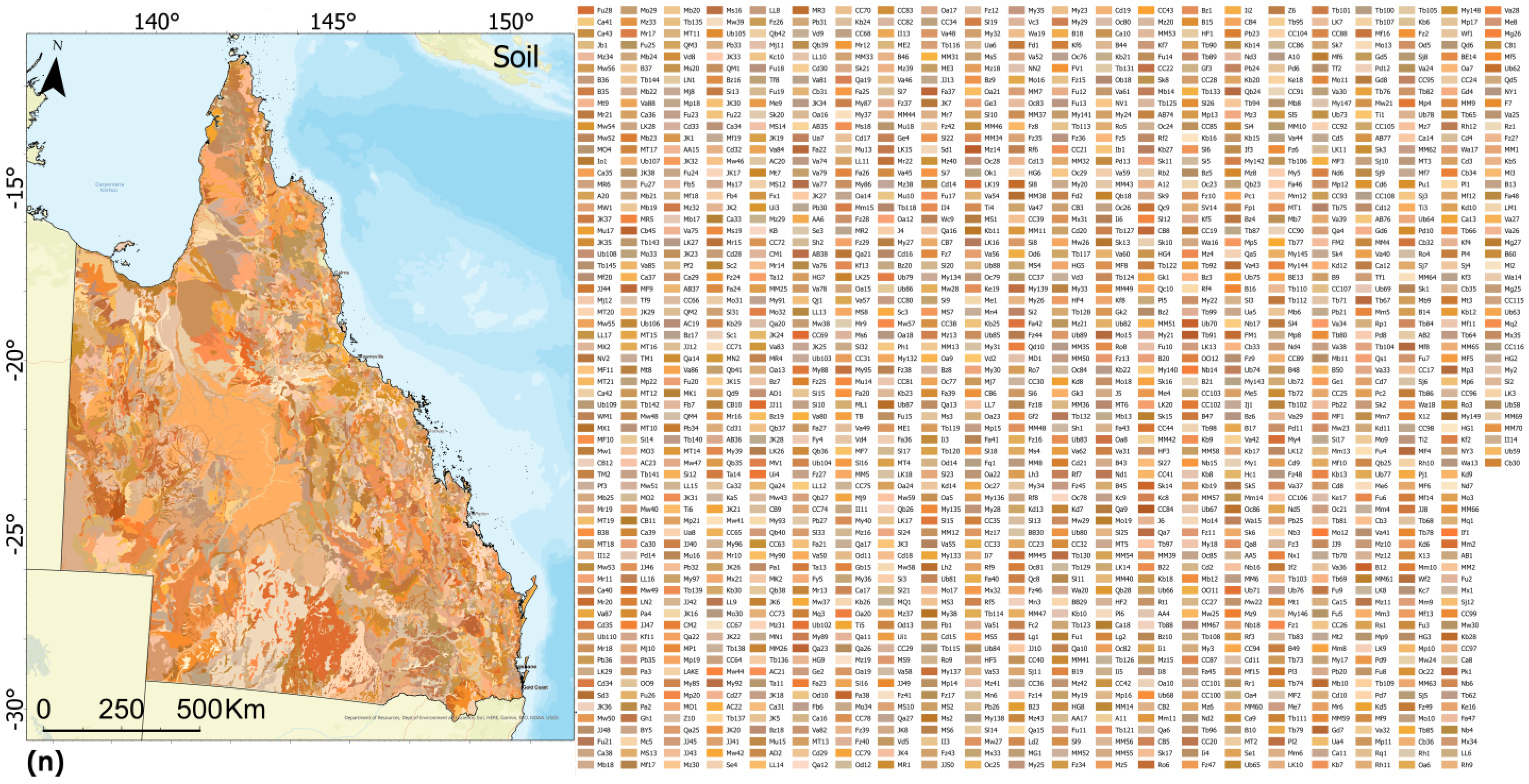
The continuity of fire in the area can be interrupted by linear features such as rivers and roads [57]. Therefore, distance to the road (Figure 4g) and distance to the river (Figure 4h) factors were used in the assessment. Rainfall (Figure 4i) and wind (Figure 4j) are two of the most influential wildfire conditioning factors which affect wildfire generation and extension [58,59]. Rainfall affects fuel moisture, and wind controls the direction and extent of the wildfire. Cumming [60] stated that two determinants of fire behavior are weather and spatial variation in forest types. Hence, forest types (Figure 4k) across QLD were included. LULC, geology and soil, as other wildfire conditioning factors, are illustrated in Figure 4l–n, respectively. The dataset was prepared by converting all the factors to raster format with a 5 × 5 m cell size. Regarding the scale of soil and geology, although the original pixel sizes of soil and geology layers were greater than 5 m they covered large areas with no sudden changes in those classes. Therefore, they were resampled to 5 × 5 m cell size as well in order to keep the consistency in the dataset.
In studies such as natural hazards, in which a variety of factors are involved, assessment of multicollinearity among conditioning factors is an essential task [61]. It is defined as multicollinearity when having near-linear relationships among wildfire conditioning factors [62]. Performing the analysis before solving the multicollinearity problem could lead to inaccurate outcomes. To handle multicollinearity, it is important to recognize its sources. Tolerance (TOL) and variance inflation (VIF) factors are the two most popular and highly effective methods to justify multicollinearity between the various factors [63]. In this study, the VIF and TOL methods were used to check for multicollinearity of the conditioning factors. In multicollinearity analysis, a VIF greater than 5, or a tolerance smaller than 0.2 shows the existence of a multicollinearity problem [64]. Therefore, the factors with these values should be removed from the dataset [42].

3.1.3. Vulnerability-Related Factors

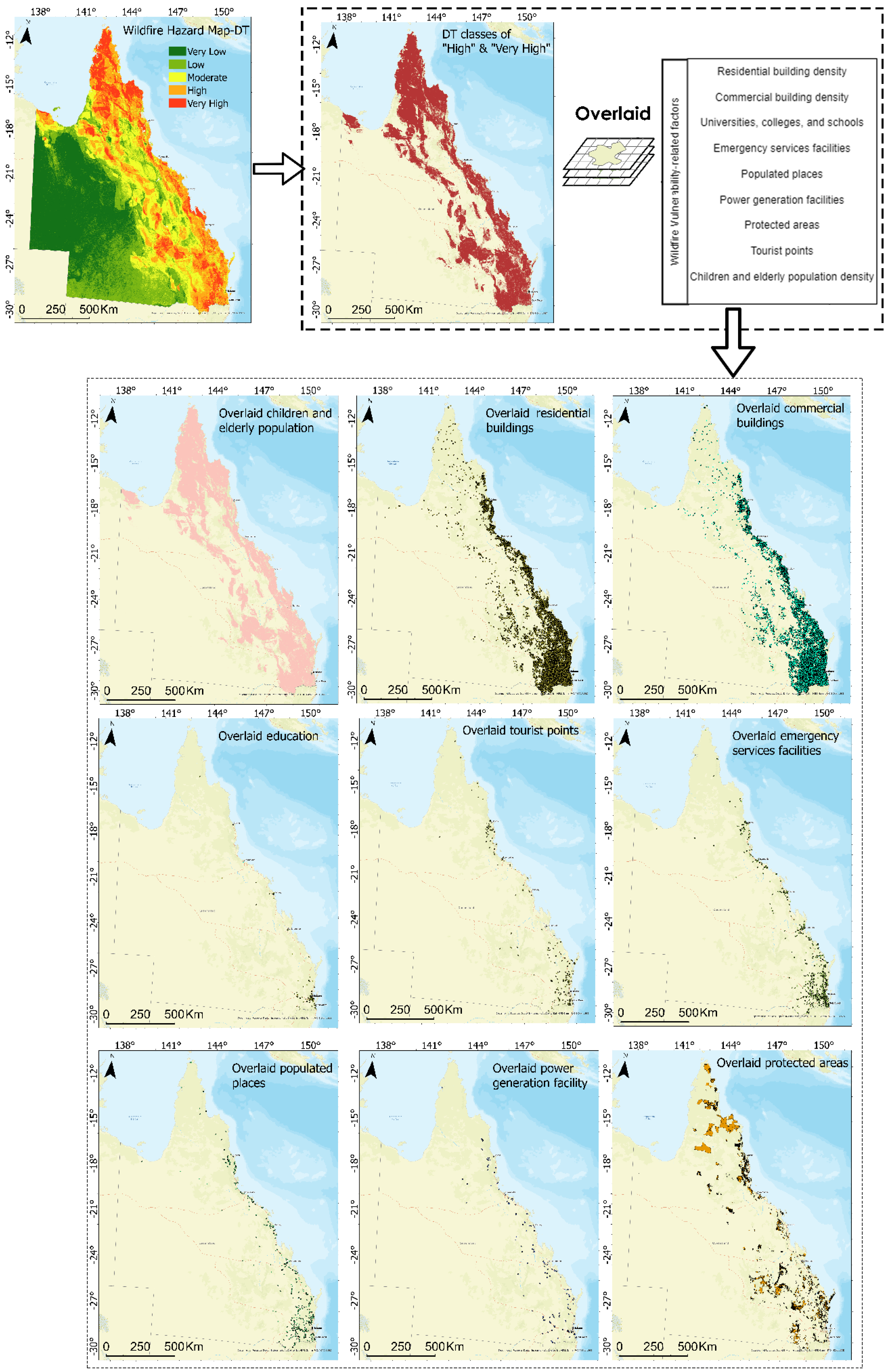
Figure 5 is a schematic presentation of the wildfire vulnerability-related factors. By overlaying the hazard map over these factors, their relation to fire danger can be estimated. First, each factor was ranked according to the literature from zero to five, with five being the highest and zero being the lowest vulnerability. This dataset includes children and elderly population density (Figure 5a), residential building density (Figure 5b), commercial building density (Figure 5c), education (Figure 5d), tourist points (Figure 5e), emergency service facilities (Figure 5f), populated places (Figure 5g), power generation facilities (Figure 5h) and protected areas (Figure 5i). The “children and elderly population density” factor was prepared using children younger than five years old and elderly above sixty years old. The factors of “children and elderly population density”, “residential building density,” and “commercial building density” were created using the kernel density tool in the ArcGIS environment. A higher density represents greater vulnerability. Figure 5d represents the schools, colleges, and universities in QLD. Figure 5d and the rest of the figures were produced using the Euclidean distance tool. The closer to these features the higher the vulnerability. Similar to wildfire hazard-related factors, all factors were generated with 5 × 5 m cell size.

3.2. Hazard Assessment

The general assumption in wildfire prediction is that future wildfires will occur under the same conditions as past wildfires. According to this assumption, the correlation between wildfires happening in a region and wildfire hazard-related factors needs to be evaluated. In this research, two well-known ML methods have been used to perform the hazard analysis which will be described below.

3.2.1. Decision Tree (DT)

One of the most popular supervised learning algorithms is DT [65], which is able to perform both classification and regression analysis [66]. A DT consists of if-then-else rules with multiple branches joined by decision nodes and terminated by leaf nodes. The decision node is where the tree splits into various branches. Each branch is related to the specific decision made by the algorithm, and leaf nodes show the output of the model [67]. This could be a label for a classification problem or a continuous value in the case of a regression problem. DT divides the dataset into groups so that each group holds more or less homogeneous states of the target variable (wildfire). At each splitting step, all attributes related to the conditioning factors are evaluated for their influence on wildfire occurrence. The recursive process continues and once completed, the final decision tree is shaped [68]. Chi-square automatic interaction detection (CHAID) [69] is one of the DT algorithms that perform Dodge separation using the chi-square test (categorical target variable) or F-test (continuous target variable). Pearson’s chi-square statistic or likelihood ratio chi-square statistic is used in the CHAID algorithm as a separation criterion in case the target variable is categorical (current case of wildfire). This algorithm was used to perform DT and consists of three steps: merging, splitting, and stopping.

3.2.2. Support Vector Machines (SVMs)

Another popular supervised learning algorithm is SVM [70]. SVM is a classifier that determines the hyperplane, a decision boundary in an n-dimensional space separating the boundary of each class, for data in n dimensions [71]. The optimal hyperplane is based on the distance between the nearest point of each class, and the decision boundary is maximized. If it is possible to separate the data by a line, then the hyperplane can be defined as W T x + b = 0 , where the w is the weight vector, x is the input vector, and b is the bias. The distance of the hyperplane to the closest data point d, called a support vector, is defined as the margin of separation. The main objective is to recognize the optimal hyperplane that minimizes the margin. If the data are not linearly separable, kernel SVM methods first apply a set of transformations to the data to a higher dimensional space where finding this hyperplane is easier. The classification decision function is expressed as:
g ( x ) = s i g n   ( i = 1 n y i α j K ( x i , x j ) + b )
where K ( x i , x j ) is the kernel function. Radial basic function (RBF) was used to perform SVM, which is one of the kernels most often used due to its proficiency and precision.

3.3. Vulnerability Assessment

As described in Section 3.1.3, vulnerability-related factors were ranked and prepared in an index format from 0 to 1. Table 2 listed the factors and their assigned weights. In the case of density factors such as residential building density, the denser the area, the higher the vulnerability. Regarding distance-related factors, for all except “emergency services facilities,” the vulnerability decreases with increasing distance. The vulnerability stage was assessed by overlaying factors that weighted the areas according to the level of vulnerability.

3.4. Risk Assessment

Natural hazard risk is usually defined as the combination of hazard potential and vulnerability [72]:
Risk = Hazard potential × Vulnerability
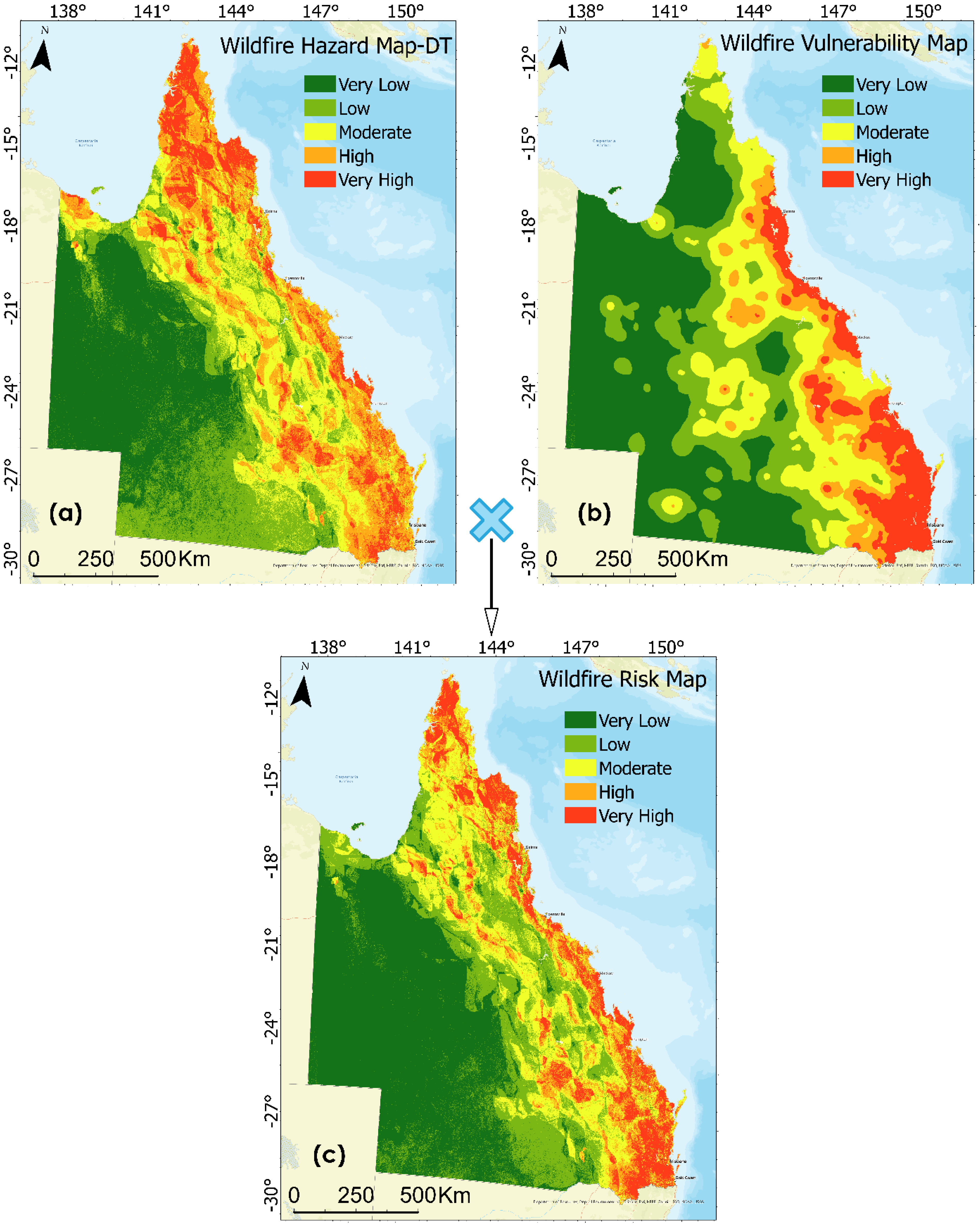
The derived wildfire hazard map was normalized to be from 0 to 1. Finally, a wildfire risk map was generated by multiplying hazard and vulnerability. For statistical purposes, the wildfire risk map for QLD was represented in five categories produced by quantile method as follows: “very high”, “high”, “moderate”, “low” and “very low” risk.

Validation

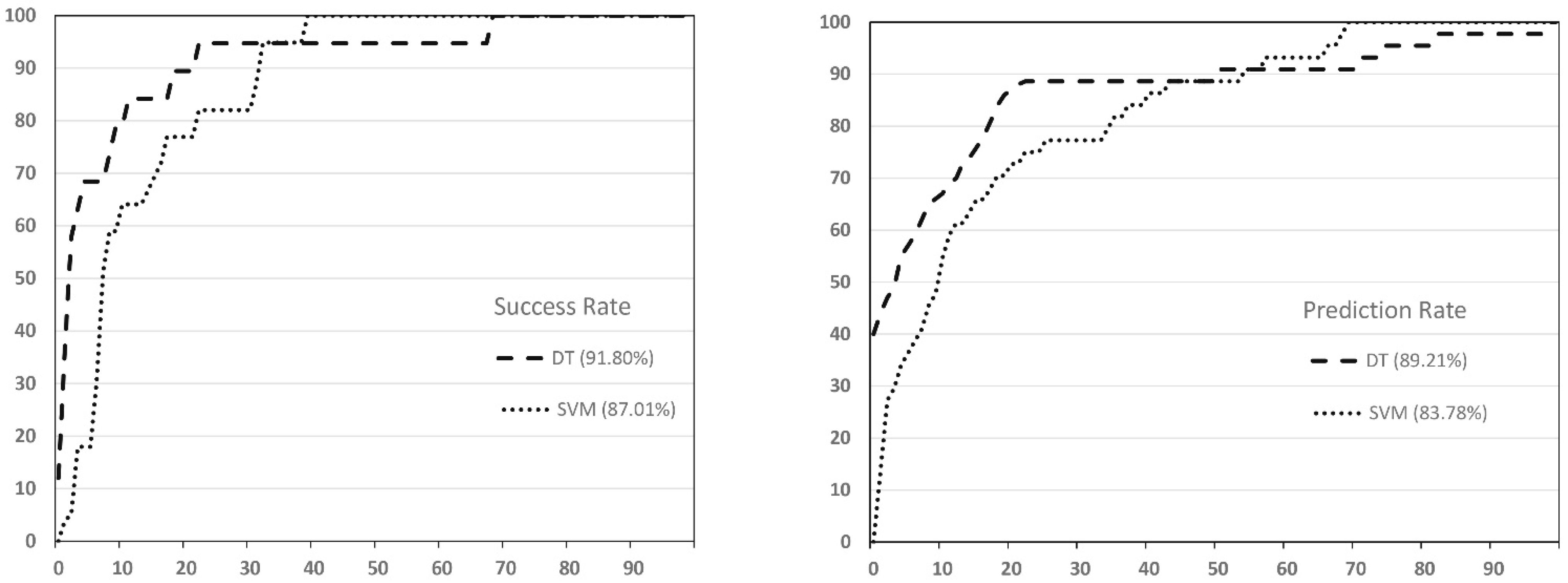
One of the important stages in susceptibility analysis and evaluating its quality is validation [73]. Especially in prediction modeling, it is critical to validate predicted outcomes so that outputs provide a meaningful interpretation concerning wildfire susceptibility [74]. The area under the curve (AUC) is a well-known method used to evaluate the correctness and reliability of wildfire susceptibility maps. AUC wildfire training and testing datasets were used to validate the results by measuring the corresponding success rates and prediction rates [75]. The success rate was measured using the training points; however, the prediction rate was that of the remaining testing wildfire points. The testing points represent independent information not used in the modeling.
The process starts by sorting the calculated wildfire hazard index values in descending order. Subsequently, those values are classified using an equal interval tool into 100 classes with 1% cumulative intervals. The classified wildfire hazard maps were crossed with the wildfire inventory maps (training and testing). Doing so, success and prediction rate curves were measured from the cross-table values and represented as continuous lines. Cumulative plots of the percentage of wildfire occurrences versus cumulative 1% equal area of ordered hazard ranks were created to measure the AUC value for each curve. To compare the results quantitatively, the areas under the curves were re-calculated with the total area equal to 100. The validation output for both methods was calculated and compared. The method with the highest AUC was selected for use in the rest of the analysis.

4. Results and Discussion

To start, multicollinearity was detected by calculating VIF and TOL for each wildfire conditioning factor. Table 3 lists the measured VIF and TOL and, according to the results, there were multicollinearity problems in the dataset. The problem was related to the factors of curvature and soil which had VIF values >5 and tolerance <0.2. Multicollinearity was corrected by omitting these factors from the dataset.
The relationships between wildfire occurrence and hazard-related factors have been evaluated using DT and SVM. The produced maps were reclassified into five classes by quantile for ease of visual interpretation. Figure 6 illustrates the final hazard maps. As can be seen in both figures, the north and southeast parts of the study area have been recognized as very highly hazardous zones. However, the hazardous areas around QLD detected by DT are more than SVM in terms of coverage. The correctness of these methods was evaluated through accuracy assessment.
The outcomes of the wildfire hazard mapping were evaluated by comparing them with the existing wildfire locations. The AUC method was applied and both success and prediction rates were calculated. The success rate was measured by comparing the wildfire grid cells (210 cells) in the training dataset with the DT and SVM wildfire hazard maps. The success rate shows how the wildfire hazard outcomes fit the training dataset. Since the training dataset was used for training the DT and SVM model, it may not be a precise approach to assess the prediction capacity of the methods. The prediction rate is a suitable way to test how well the wildfire models and wildfire conditioning factors predict possible future wildfire areas. The wildfire grid cells that were not used in the training process (90 cells) were used to measure the prediction rate. For both success and prediction rates, if the AUC is equal to 100 it represents perfect accuracy. The AUC values (Figure 7) obtained from two hazard maps revealed that DT showed the highest success and prediction rates (91.80% and 89.21%, respectively). The SVM success rate (87.01%) was close to the DT success rate; however, SVM’s prediction rate (83.78%) was 6% lower than that of DT. In fact, both methods provided reasonable accuracies; however, DT results were used in risk assessment due to their better performance. The proficiency of ML methods has been proven by the literature as well. Ghorbanzadeh, et al. [76], Gholamnia, et al. [77], Watson, et al. [78] are some examples of studies in which ML methods were utilized in the same field of research. Among the majority of the assessed research, ML provided the most reliable outcomes compared to other techniques. A study by Jain, Coogan, Subramanian, Crowley, Taylor and Flannigan [33] reviewed ML applications in wildfire science and management. According to their comprehensive study, the advantages of ML methods make them suitable for use in a variety of wildfire problem domains such as fire recognition and mapping, climate change and its impact on fire weather, wildfire hazard and risk, wildfire prediction, impacts of wildfire, and wildfire management. Their study is not limited to positive aspects but also discusses the limitations of various ML approaches related to the size of the dataset, analysis requirements, generalizability, and interpretability. More than forty ML algorithms were mentioned in their research. However, SVM and DT were among the most robust techniques in wildfire studies.
Although the advantages of individual ML methods are apparent, ensemble/hybrid ML techniques could enhance their strength. Mohajane, et al. [79] is one of the studies that tested hybrid DT and SVM using frequency ratio. Their outcomes showed that their developed hybrid models can increase the accuracy and performance of wildfire susceptibility studies. Therefore, for future analysis, ensemble modeling and its impact on the final outputs was considered as well.
As an additional step, classes of “High” and “Very High” derived from DT were extracted and overlaid with vulnerability feature maps to visually assess their vulnerability. Figure 8 shows that many of these features are located in high and very high susceptible zones. As can be seen visually, many of the features are located in these zones.
To create the final wildfire vulnerability map, all weighted and normalized vulnerability-related factors were overlaid, and a vulnerability map was created using Raster Calculator in a GIS environment. The vulnerability maps had classifications of “very high”, “high”, “moderate”, “low” and “very low” as illustrated in Figure 9b. As the final step, the derived hazard (Figure 9a) and vulnerability maps were multiplied, and a wildfire risk map has been created (Figure 9c)
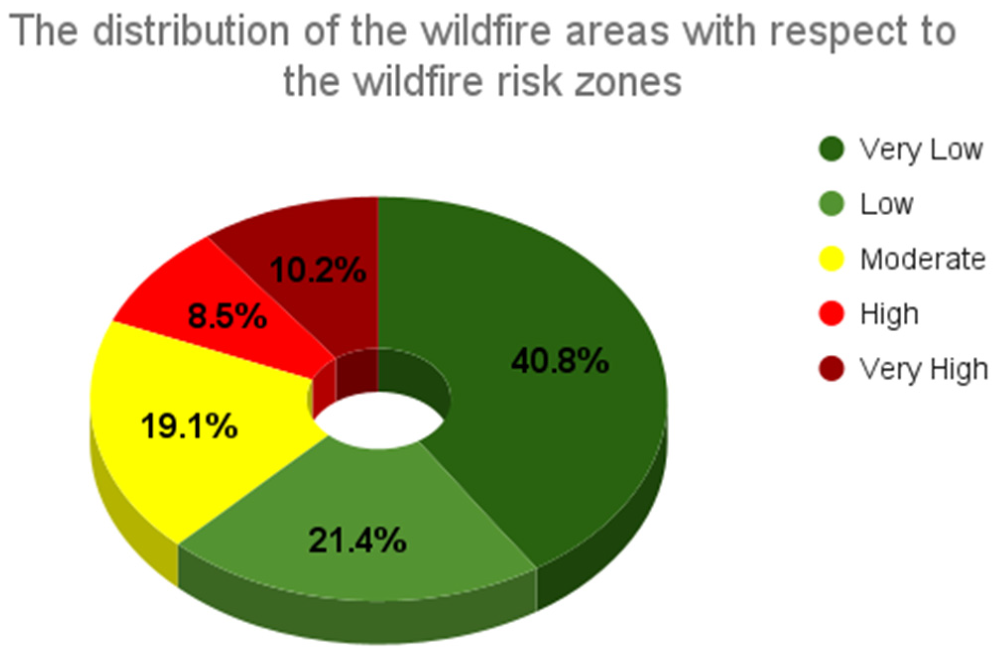
It is apparent that high wildfire risk areas have many settlements, and in these regions the probability of wildfire occurrence is very high. Risky regions must be brought to the notice of the government and public so that they are aware of future wildfire possibilities. Doing so, lots of lives and properties could be saved. Figure 10 also illustrates the distribution of wildfire areas with respect to wildfire risk areas. It shows that 10.2% and 8.5% of QLD is located in “very high” and “high” risk zones respectively.
According to the literature, the majority of people living in high wildfire-risk areas are aware of their exposure. However, this does not mean that they try to act to mitigate risks. The 2009 Black Saturday fires in Victoria are a good example in which most people understood about the risky areas, but only a few took action when the highest-level warning was issued. Therefore, all parties in society (academics, governments, and citizens) have to work together to achieve optimal mitigation actions (Haque et al., 2021 [1]). It should be taken into consideration that not only human life, but also a wide range of species, can be affected by wildfire. Especially in QLD, due to a range of threatening processes, some species are decreasing in numbers and are at risk of extinction. For instance, on 30 April 2021, there were 1020 threatened species (236 animals and 784 plants) listed as threatened under the Queensland Nature Conservation Act 1992. Therefore, it is necessary to consider all possible damage, recognize risky areas, conduct comprehensive education, and plan wisely to control this disaster.
Regarding the limitations of this study and possible improvement, the output of this study could be more precise if projected climate change was available for use in the analysis. The reason is that global warming and other climatic factors constantly change and can considerably affect future wildfire occurrences.

5. Conclusions

Wildfire risk analysis can help scientists and managers better understand the timing, location, and potential effects of wildfires on economic and ecological systems. It can address forest management issues and disclose tradeoffs that other analysis techniques may not account for. This study focused on areas with high wildfire risk in QLD, Australia, to provide proper knowledge for scientists and citizens. Two datasets of wildfire hazard-related factors and vulnerability-related factors were prepared and used in the analysis. DT and SVM were applied to assess the hazard and extract the correlation between wildfire conditioning factors and wildfire inventory. Using AUC, optimal accuracy was achieved from DT with 89.21% prediction accuracy. Therefore, the output from DT was used in the rest of the analysis. Vulnerability-related factors were ranked and prepared as an index from 0 to 1. The ranking factors were then overlaid to extract vulnerability areas. Finally, both the DT-derived hazard map and vulnerability map combined to create the risk map. Results revealed that most the urban regions in QLD are at high risk of wildfire. These areas need proper mitigation action to avoid or minimize future wildfire damage. In conclusion, regardless of the surrounding ecosystem conditions, all communities can better coexist with fire by participating in risk awareness and continuing education.

Funding

This research received no external funding.

Institutional Review Board Statement

Not applicable.

Informed Consent Statement

Not applicable.

Data Availability Statement

Not applicable.

Conflicts of Interest

The author declares no conflict of interest.

References

  1. Haque, M.K.; Azad, M.A.K.; Hossain, M.Y.; Ahmed, T.; Uddin, M.; Hossain, M.M. Wildfire in Australia during 2019–2020, Its Impact on Health, Biodiversity and Environment with Some Proposals for Risk Management: A Review. J. Environ. Prot. 2021, 12, 391–414. [Google Scholar] [CrossRef]
  2. Moreira, F.; Ascoli, D.; Safford, H.; Adams, M.A.; Moreno, J.M.; Pereira, J.M.; Catry, F.X.; Armesto, J.; Bond, W.; González, M.E. Wildfire management in Mediterranean-type regions: Paradigm change needed. Environ. Res. Lett. 2020, 15, 011001. [Google Scholar] [CrossRef]
  3. Schulze, S.S.; Fischer, E.C.; Hamideh, S.; Mahmoud, H. Wildfire impacts on schools and hospitals following the 2018 California Camp Fire. Nat. Hazards 2020, 104, 901–925. [Google Scholar] [CrossRef]
  4. Moritz, M.A.; Batllori, E.; Bradstock, R.A.; Gill, A.M.; Handmer, J.; Hessburg, P.F.; Leonard, J.; McCaffrey, S.; Odion, D.C.; Schoennagel, T. Learning to coexist with wildfire. Nature 2014, 515, 58–66. [Google Scholar] [CrossRef] [PubMed]
  5. Miller, C.; Ager, A.A. A review of recent advances in risk analysis for wildfire management. Int. J. Wildland Fire 2012, 22, 1–14. [Google Scholar] [CrossRef] [Green Version]
  6. Safronov, A.N. Spatio-Temporal Assessment of Thunderstorms’ Effects on Wildfire in Australia in 2017–2020 Using Data from the ISS LIS and MODIS Space-Based Observations. Atmosphere 2022, 13, 662. [Google Scholar] [CrossRef]
  7. Abram, N.J.; Henley, B.J.; Sen Gupta, A.; Lippmann, T.J.; Clarke, H.; Dowdy, A.J.; Sharples, J.J.; Nolan, R.H.; Zhang, T.; Wooster, M.J. Connections of climate change and variability to large and extreme forest fires in southeast Australia. Commun. Earth Environ. 2021, 2, 8. [Google Scholar] [CrossRef]
  8. Harris, S.; Lucas, C. Understanding the variability of Australian fire weather between 1973 and 2017. PLoS ONE 2019, 14, e0222328. [Google Scholar] [CrossRef]
  9. Bowman, D.M.; Williamson, G.J.; Abatzoglou, J.T.; Kolden, C.A.; Cochrane, M.A.; Smith, A. Human exposure and sensitivity to globally extreme wildfire events. Nat. Ecol. Evol. 2017, 1, 0058. [Google Scholar] [CrossRef]
  10. Van Oldenborgh, G.J.; Krikken, F.; Lewis, S.; Leach, N.J.; Lehner, F.; Saunders, K.R.; Van Weele, M.; Haustein, K.; Li, S.; Wallom, D. Attribution of the Australian bushfire risk to anthropogenic climate change. Nat. Hazards Earth Syst. Sci. 2021, 21, 941–960. [Google Scholar] [CrossRef]
  11. Davey, S.M.; Sarre, A. The 2019/20 Black Summer Bushfires; Taylor & Francis: Abingdon, UK, 2020; Volume 83, pp. 47–51. [Google Scholar]
  12. Pryor, L.; Woolacott, J. Surviving the Australian Black Summer bushfires: A veterinary perspective. Livestock 2021, 26, 26–29. [Google Scholar] [CrossRef]
  13. Tin, D.; Hertelendy, A.J.; Ciottone, G.R. What we learned from the 2019–2020 Australian Bushfire disaster: Making counter-terrorism medicine a strategic preparedness priority. Am. J. Emerg. Med. 2020, 46, 742–743. [Google Scholar] [CrossRef] [PubMed]
  14. McWethy, D.B.; Schoennagel, T.; Higuera, P.E.; Krawchuk, M.; Harvey, B.J.; Metcalf, E.C.; Schultz, C.; Miller, C.; Metcalf, A.L.; Buma, B. Rethinking resilience to wildfire. Nat. Sustain. 2019, 2, 797–804. [Google Scholar] [CrossRef]
  15. Gill, A.M.; Stephens, S.L.; Cary, G.J. The worldwide “wildfire” problem. Ecol. Appl. 2013, 23, 438–454. [Google Scholar] [CrossRef] [PubMed] [Green Version]
  16. Alexander, D. Natural Disasters; Routledge: Oxfordshire, UK, 2018. [Google Scholar]
  17. Shah, M.A.R.; Renaud, F.G.; Anderson, C.C.; Wild, A.; Domeneghetti, A.; Polderman, A.; Votsis, A.; Pulvirenti, B.; Basu, B.; Thomson, C. A review of hydro-meteorological hazard, vulnerability, and risk assessment frameworks and indicators in the context of nature-based solutions. Int. J. Disaster Risk Reduct. 2020, 50, 101728. [Google Scholar] [CrossRef]
  18. Gervasi, O.; Murgante, B.; Misra, S.; Garau, C.; Blečić, I.; Taniar, D.; Apduhan, B.O.; Rocha, A.M.A.; Tarantino, E.; Torre, C.M. Computational Science and Its Applications–ICCSA 2021: 21st International Conference, Cagliari, Italy, 13–16 September 2021, Proceedings, Part VI; Springer Nature: Berlin/Heidelberg, Germany, 2021; Volume 12954. [Google Scholar]
  19. Cardona, O.D.; Van Aalst, M.K.; Birkmann, J.; Fordham, M.; Mc Gregor, G.; Rosa, P.; Pulwarty, R.S.; Schipper, E.L.F.; Sinh, B.T.; Décamps, H. Determinants of risk: Exposure and vulnerability. In Managing the Risks of Extreme Events and Disasters to Advance Climate Change Adaptation: Special Report of the Intergovernmental Panel on Climate Change; Cambridge University Press: Cambridge, UK, 2012; pp. 65–108. [Google Scholar]
  20. Chuvieco, E.; Aguado, I.; Yebra, M.; Nieto, H.; Salas, J.; Martín, M.P.; Vilar, L.; Martínez, J.; Martín, S.; Ibarra, P. Development of a framework for fire risk assessment using remote sensing and geographic information system technologies. Ecol. Model. 2010, 221, 46–58. [Google Scholar] [CrossRef]
  21. Jaafari, A.; Termeh, S.V.R.; Bui, D.T. Genetic and firefly metaheuristic algorithms for an optimized neuro-fuzzy prediction modeling of wildfire probability. J. Environ. Manag. 2019, 243, 358–369. [Google Scholar] [CrossRef]
  22. Jaafari, A.; Zenner, E.K.; Panahi, M.; Shahabi, H. Hybrid artificial intelligence models based on a neuro-fuzzy system and metaheuristic optimization algorithms for spatial prediction of wildfire probability. Agric. For. Meteorol. 2019, 266, 198–207. [Google Scholar] [CrossRef]
  23. Pourghasemi, H.r.; Beheshtirad, M.; Pradhan, B. A comparative assessment of prediction capabilities of modified analytical hierarchy process (M-AHP) and Mamdani fuzzy logic models using Netcad-GIS for forest fire susceptibility mapping. Geomat. Nat. Hazards Risk 2016, 7, 861–885. [Google Scholar] [CrossRef] [Green Version]
  24. Ghorbanzadeh, O.; Blaschke, T. Wildfire susceptibility evaluation by integrating an analytical network process approach into GIS-based analyses. In Proceedings of the ISERD International Conference, Toronto, ON, Canada, 28–29 June 2018. [Google Scholar]
  25. Kaku, K.; Honma, T.; Fukuda, M. An Application of AHP/ANP to A Wildfire Management Project to Help Mitigate Global Warming. In Proceedings of the International Symposium on the Analytic Hierarchy Process, Pittsburgh, PA, USA, 29 July–1 August 2009. [Google Scholar]
  26. Vilar del Hoyo, L.; Martín Isabel, M.P.; Martínez Vega, F.J. Logistic regression models for human-caused wildfire risk estimation: Analysing the effect of the spatial accuracy in fire occurrence data. Eur. J. For. Res. 2011, 130, 983–996. [Google Scholar] [CrossRef]
  27. Chen, W.; Zhao, X.; Shahabi, H.; Shirzadi, A.; Khosravi, K.; Chai, H.; Zhang, S.; Zhang, L.; Ma, J.; Chen, Y. Spatial prediction of landslide susceptibility by combining evidential belief function, logistic regression and logistic model tree. Geocarto Int. 2019, 34, 1177–1201. [Google Scholar] [CrossRef]
  28. Tehrany, M.S.; Özener, H.; Kalantar, B.; Ueda, N.; Habibi, M.R.; Shabani, F.; Saeidi, V.; Shabani, F. Application of an ensemble statistical approach in spatial predictions of bushfire probability and risk mapping. J. Sens. 2021, 2021, 6638241. [Google Scholar] [CrossRef]
  29. Yue, X.; Mickley, L.J.; Logan, J.A.; Kaplan, J.O. Ensemble projections of wildfire activity and carbonaceous aerosol concentrations over the western United States in the mid-21st century. Atmos. Environ. 2013, 77, 767–780. [Google Scholar] [CrossRef] [PubMed] [Green Version]
  30. Mojaddadi, H.; Pradhan, B.; Nampak, H.; Ahmad, N.; Ghazali, A.H.B. Ensemble machine-learning-based geospatial approach for flood risk assessment using multi-sensor remote-sensing data and GIS. Geomat. Nat. Hazards Risk 2017, 8, 1080–1102. [Google Scholar] [CrossRef] [Green Version]
  31. Asim, K.; Martínez-Álvarez, F.; Basit, A.; Iqbal, T. Earthquake magnitude prediction in Hindukush region using machine learning techniques. Nat. Hazards 2017, 85, 471–486. [Google Scholar] [CrossRef]
  32. Hosseini, F.S.; Choubin, B.; Mosavi, A.; Nabipour, N.; Shamshirband, S.; Darabi, H.; Haghighi, A.T. Flash-flood hazard assessment using ensembles and Bayesian-based machine learning models: Application of the simulated annealing feature selection method. Sci. Total Environ. 2020, 711, 135161. [Google Scholar] [CrossRef]
  33. Jain, P.; Coogan, S.C.; Subramanian, S.G.; Crowley, M.; Taylor, S.; Flannigan, M.D. A review of machine learning applications in wildfire science and management. Environ. Rev. 2020, 28, 478–505. [Google Scholar] [CrossRef]
  34. Chapelle, O.; Vapnik, V.; Bousquet, O.; Mukherjee, S. Choosing multiple parameters for support vector machines. Mach. Learn. 2002, 46, 131–159. [Google Scholar] [CrossRef]
  35. Willard, J.; Jia, X.; Xu, S.; Steinbach, M.; Kumar, V. Integrating physics-based modeling with machine learning: A survey. arXiv 2020, arXiv:2003.049191, 1–34. [Google Scholar]
  36. Deb, J.; Phinn, S.; Butt, N.; McAlpine, C. Climate change impacts on tropical forests: Identifying risks for tropical Asia. J. Trop. For. Sci. 2018, 30, 182–194. [Google Scholar]
  37. Bondur, V.; Voronova, O.; Gordo, K.; Zima, A.; Feoktistova, N. Satellite monitoring of multiyear wildfires and related emissions of harmful trace gases into the air environment of Australia. Izv. Atmos. Ocean. Phys. 2021, 57, 1029–1041. [Google Scholar] [CrossRef]
  38. McClure, L.; Baker, D. How do planners deal with barriers to climate change adaptation? A case study in Queensland, Australia. Landsc. Urban Plan. 2018, 173, 81–88. [Google Scholar] [CrossRef]
  39. Hu, W.; Clements, A.; Williams, G.; Tong, S.; Mengersen, K. Spatial patterns and socioecological drivers of dengue fever transmission in Queensland, Australia. Environ. Health Perspect. 2012, 120, 260–266. [Google Scholar] [CrossRef] [PubMed] [Green Version]
  40. Akter, R.; Hu, W.; Gatton, M.; Bambrick, H.; Naish, S.; Tong, S. Different responses of dengue to weather variability across climate zones in Queensland, Australia. Environ. Res. 2020, 184, 109222. [Google Scholar] [CrossRef]
  41. Hosseini, M.; Lim, S. Gene Expression Programming and Machine Learning Methods for Bushfire Susceptibility Mapping in New South Wales, Australia. Nat. Hazards 2021, 113, 1349–1365. [Google Scholar] [CrossRef]
  42. Jaafari, A.; Mafi-Gholami, D.; Thai Pham, B.; Tien Bui, D. Wildfire probability mapping: Bivariate vs. multivariate statistics. Remote Sens. 2019, 11, 618. [Google Scholar] [CrossRef] [Green Version]
  43. Eskandari, S.; Amiri, M.; Sãdhasivam, N.; Pourghasemi, H.R. Comparison of new individual and hybrid machine learning algorithms for modeling and mapping fire hazard: A supplementary analysis of fire hazard in different counties of Golestan Province in Iran. Nat. Hazards 2020, 104, 305–327. [Google Scholar] [CrossRef]
  44. Pourtaghi, Z.S.; Pourghasemi, H.R.; Aretano, R.; Semeraro, T. Investigation of general indicators influencing on forest fire and its susceptibility modeling using different data mining techniques. Ecol. Indic. 2016, 64, 72–84. [Google Scholar] [CrossRef]
  45. Verde, J.; Zêzere, J. Assessment and validation of wildfire susceptibility and hazard in Portugal. Nat. Hazards Earth Syst. Sci. 2010, 10, 485–497. [Google Scholar] [CrossRef]
  46. Ghorbanzadeh, O.; Valizadeh Kamran, K.; Blaschke, T.; Aryal, J.; Naboureh, A.; Einali, J.; Bian, J. Spatial prediction of wildfire susceptibility using field survey gps data and machine learning approaches. Fire 2019, 2, 43. [Google Scholar] [CrossRef] [Green Version]
  47. Johnston, P.; Kelso, J.; Milne, G.J. Efficient simulation of wildfire spread on an irregular grid. Int. J. Wildland Fire 2008, 17, 614–627. [Google Scholar] [CrossRef]
  48. Parente, J.; Pereira, M.G.; Tonini, M. Space-time clustering analysis of wildfires: The influence of dataset characteristics, fire prevention policy decisions, weather and climate. Sci. Total Environ. 2016, 559, 151–165. [Google Scholar] [CrossRef] [PubMed]
  49. Holden, Z.A.; Jolly, W.M. Modeling topographic influences on fuel moisture and fire danger in complex terrain to improve wildland fire management decision support. For. Ecol. Manag. 2011, 262, 2133–2141. [Google Scholar] [CrossRef]
  50. Prichard, S.J.; Kennedy, M.C. Fuel treatments and landform modify landscape patterns of burn severity in an extreme fire event. Ecol. Appl. 2014, 24, 571–590. [Google Scholar] [CrossRef]
  51. Fernández-Alonso, J.M.; Vega, J.A.; Jiménez, E.; Ruiz-González, A.D.; Álvarez-González, J.G. Spatially modeling wildland fire severity in pine forests of Galicia, Spain. Eur. J. For. Res. 2017, 136, 105–121. [Google Scholar] [CrossRef]
  52. Lambin, E.F.; Geist, H.J.; Lepers, E. Dynamics of land-use and land-cover change in tropical regions. Annu. Rev. Environ. Resour. 2003, 28, 205–241. [Google Scholar] [CrossRef] [Green Version]
  53. Guerrero, F.J.D.T.; Hinojosa-Corona, A.; Kretzschmar, T.G. A comparative study of NDVI values between north-and south-facing slopes in a semiarid mountainous region. IEEE J. Sel. Top. Appl. Earth Obs. Remote Sens. 2016, 9, 5350–5356. [Google Scholar] [CrossRef]
  54. Lee, S.; Pradhan, B. Probabilistic landslide hazards and risk mapping on Penang Island, Malaysia. J. Earth Syst. Sci. 2006, 115, 661–672. [Google Scholar] [CrossRef] [Green Version]
  55. Moore, I.D.; Grayson, R.; Ladson, A. Digital terrain modelling: A review of hydrological, geomorphological, and biological applications. Hydrol. Process. 1991, 5, 3–30. [Google Scholar] [CrossRef]
  56. Pettorelli, N.; Vik, J.O.; Mysterud, A.; Gaillard, J.-M.; Tucker, C.J.; Stenseth, N.C. Using the satellite-derived NDVI to assess ecological responses to environmental change. Trends Ecol. Evol. 2005, 20, 503–510. [Google Scholar] [CrossRef]
  57. Mahdavi, A. Forests and rangelands? wildfire risk zoning using GIS and AHP techniques. Casp. J. Environ. Sci. 2012, 10, 43–52. [Google Scholar]
  58. Slocum, M.G.; Platt, W.J.; Beckage, B.; Orzell, S.L.; Taylor, W. Accurate quantification of seasonal rainfall and associated climate–wildfire relationships. J. Appl. Meteorol. Climatol. 2010, 49, 2559–2573. [Google Scholar] [CrossRef] [Green Version]
  59. Sharples, J.J. Review of formal methodologies for wind–slope correction of wildfire rate of spread. Int. J. Wildland Fire 2008, 17, 179–193. [Google Scholar] [CrossRef]
  60. Cumming, S. Forest type and wildfire in the Alberta boreal mixedwood: What do fires burn? Ecol. Appl. 2001, 11, 97–110. [Google Scholar] [CrossRef]
  61. Siagian, T.H.; Purhadi, P.; Suhartono, S.; Ritonga, H. Social vulnerability to natural hazards in Indonesia: Driving factors and policy implications. Nat. Hazards 2014, 70, 1603–1617. [Google Scholar] [CrossRef]
  62. Banerjee, P. MODIS-FIRMS and ground-truthing-based wildfire likelihood mapping of Sikkim Himalaya using machine learning algorithms. Nat. Hazards 2022, 110, 899–935. [Google Scholar] [CrossRef]
  63. Arabameri, A.; Saha, S.; Roy, J.; Chen, W.; Blaschke, T.; Tien Bui, D. Landslide susceptibility evaluation and management using different machine learning methods in the Gallicash River Watershed, Iran. Remote Sens. 2020, 12, 475. [Google Scholar] [CrossRef] [Green Version]
  64. Kim, J.H. Multicollinearity and misleading statistical results. Korean J. Anesthesiol. 2019, 72, 558–569. [Google Scholar] [CrossRef] [Green Version]
  65. Caruana, R.; Niculescu-Mizil, A. An empirical comparison of supervised learning algorithms. In Proceedings of the 23rd International Conference on Machine Learning, Pittsburgh, PA, USA, 25–29 June 2006; pp. 161–168. [Google Scholar]
  66. Nefeslioglu, H.; Sezer, E.; Gokceoglu, C.; Bozkir, A.; Duman, T. Assessment of landslide susceptibility by decision trees in the metropolitan area of Istanbul, Turkey. Math. Probl. Eng. 2010, 2010, 901095. [Google Scholar] [CrossRef] [Green Version]
  67. Yeon, Y.-K.; Han, J.-G.; Ryu, K.H. Landslide susceptibility mapping in Injae, Korea, using a decision tree. Eng. Geol. 2010, 116, 274–283. [Google Scholar] [CrossRef]
  68. Gralewicz, N.J.; Nelson, T.A.; Wulder, M.A. Factors influencing national scale wildfire susceptibility in Canada. For. Ecol. Manag. 2012, 265, 20–29. [Google Scholar] [CrossRef]
  69. Park, S.-J.; Lee, C.-W.; Lee, S.; Lee, M.-J. Landslide susceptibility mapping and comparison using decision tree models: A Case Study of Jumunjin Area, Korea. Remote Sens. 2018, 10, 1545. [Google Scholar] [CrossRef] [Green Version]
  70. Noble, W.S. What is a support vector machine? Nat. Biotechnol. 2006, 24, 1565–1567. [Google Scholar] [CrossRef]
  71. Chamasemani, F.F.; Singh, Y.P. Multi-class support vector machine (SVM) classifiers--an application in hypothyroid detection and classification. In Proceedings of the 2011 Sixth International Conference on Bio-Inspired Computing: Theories and Applications, Penang, Malaysia, 27–29 September 2011; pp. 351–356. [Google Scholar]
  72. Kumpulainen, S. Vulnerability concepts in hazard and risk assessment. Spec. Pap.-Geol. Surv. Finl. 2006, 42, 65. [Google Scholar]
  73. Bui, D.T.; Lofman, O.; Revhaug, I.; Dick, O. Landslide susceptibility analysis in the Hoa Binh province of Vietnam using statistical index and logistic regression. Nat. Hazards 2011, 59, 1413–1444. [Google Scholar] [CrossRef]
  74. Pourghasemi, H.R. GIS-based forest fire susceptibility mapping in Iran: A comparison between evidential belief function and binary logistic regression models. Scand. J. For. Res. 2016, 31, 80–98. [Google Scholar] [CrossRef]
  75. Rasyid, A.R.; Bhandary, N.P.; Yatabe, R. Performance of frequency ratio and logistic regression model in creating GIS based landslides susceptibility map at Lompobattang Mountain, Indonesia. Geoenviron. Disasters 2016, 3, 19. [Google Scholar] [CrossRef] [Green Version]
  76. Ghorbanzadeh, O.; Blaschke, T.; Gholamnia, K.; Aryal, J. Forest fire susceptibility and risk mapping using social/infrastructural vulnerability and environmental variables. Fire 2019, 2, 50. [Google Scholar] [CrossRef] [Green Version]
  77. Gholamnia, K.; Gudiyangada Nachappa, T.; Ghorbanzadeh, O.; Blaschke, T. Comparisons of diverse machine learning approaches for wildfire susceptibility mapping. Symmetry 2020, 12, 604. [Google Scholar] [CrossRef] [Green Version]
  78. Watson, G.L.; Telesca, D.; Reid, C.E.; Pfister, G.G.; Jerrett, M. Machine learning models accurately predict ozone exposure during wildfire events. Environ. Pollut. 2019, 254, 112792. [Google Scholar] [CrossRef]
  79. Mohajane, M.; Costache, R.; Karimi, F.; Pham, Q.B.; Essahlaoui, A.; Nguyen, H.; Laneve, G.; Oudija, F. Application of remote sensing and machine learning algorithms for forest fire mapping in a Mediterranean area. Ecol. Indic. 2021, 129, 107869. [Google Scholar] [CrossRef]
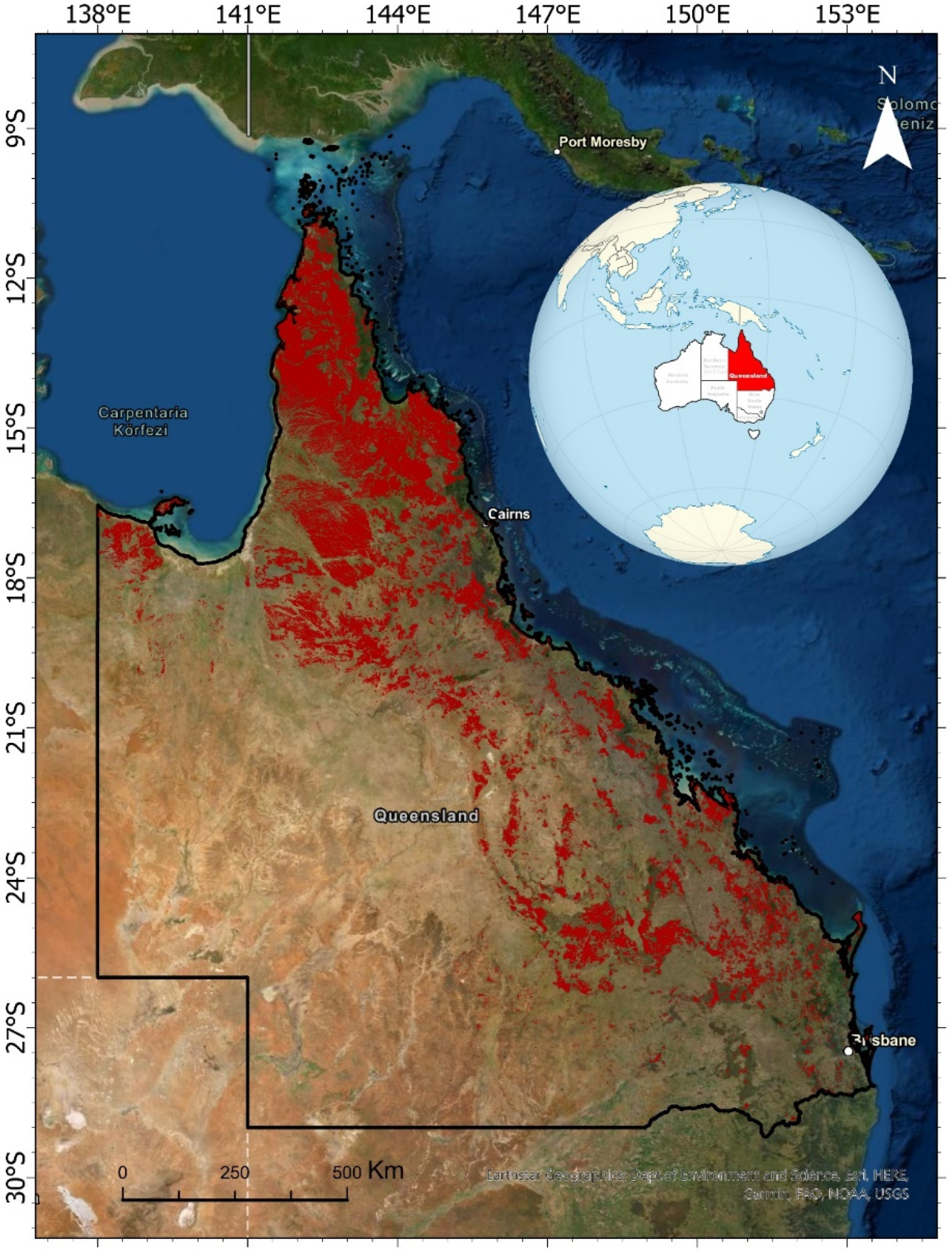
Figure 1. Study area with wildfire locations from 2011 to 2019.
Fire 06 00022 g001
Figure 2. Wildfire history in Queensland, Australia. Source: https://qldspatial.information.qld.gov.au/catalogue/custom/detail.page?fid={607736AE-8F4C-4058-B97F-CF617413EC3E}, accessed on 16 November 2021.
Fire 06 00022 g002
Figure 3. Methodology flowchart.
Fire 06 00022 g003
Figure 4. Influencing factors consisting of (a) altitude, (b) slope, (c) aspect, (d) curvature, (e) TWI, (f) NDVI, (g) distance to road, (h) distance to river, (i) rainfall, (j) wind, (k) forest types, (l) LULC, (m) geology, and (n) soil.
Fire 06 00022 g004aFire 06 00022 g004bFire 06 00022 g004c
Figure 5. Vulnerability−related factors.
Fire 06 00022 g005
Figure 6. Wildfire hazard maps.
Fire 06 00022 g006
Figure 7. AUC.
Figure 7. AUC.
Fire 06 00022 g007
Figure 8. Overlaid vulnerability-related factors with “high” and “very high” wildfire susceptibility classes.
Fire 06 00022 g008
Figure 9. Wildfire risk map.
Fire 06 00022 g009
Figure 10. Distribution of wildfire areas concerning the wildfire risk areas.
Fire 06 00022 g010
Table 1. Data source related to each dataset.
Forest Fire Extent
Queensland Government Website-Queensland Spatial Catalogue
(https://qldspatial.information.qld.gov.au/catalogue/, accessed on 22 June 2020)
Hazard-related factors
FactorSource
Altitude5-m spatial resolution (produced from LiDAR data)
SlopeDerived from altitude
AspectDerived from altitude
CurvatureDerived from altitude
Topographic wetness index (TWI)Derived from altitude
WindGlobal Wind Atlas https://globalwindatlas.info/area/Australia, accessed on 1 January 2020
Rainfallmeteorological stations. http://www.bom.gov.au/climate/data/index.shtml, accessed on 1 January 2020
Distance from riversQueensland Government Wetlands Info Website
https://www.qld.gov.au/, accessed on 1 January 2020
Distance from roadsOpenStreetMap
Soil types (1:250,000 scale)Australian Soil Resource Information System (ASRIS) https://www.asris.csiro.au/themes/Atlas.html, accessed on 1 January 2020
LULCQueensland Land Use Mapping Program (QLUMP)
Forest typesDepartment of Agriculture, Fisheries and Forestry (ABARES)
Geology (1:100,000 scale) CSIRO and Australian government websites;
http://www.ga.gov.au/data-pubs/maps, accessed on 1 January 2020
NDVILandsat imagery
Vulnerability-related factors
FactorSource
  • Residential building density
  • Commercial building density
  • Universities, colleges, and schools
  • Emergency services facilities
  • Populated places
  • Power generation facilities
  • Protected areas
  • Tourist points
Queensland Government Website-Queensland Spatial Catalogue
(https://qldspatial.information.qld.gov.au/catalogue/, accessed on 1 January 2022)
Children and elderly population densityThe Humanitarian Data Exchange Website
https://data.humdata.org/, accessed on 1 January 2022
Table 2. Ranking the vulnerability related factors.
Vulnerability Related FactorsVulnerability
Children and elderly population density1 indicates the highest vulnerability
Residential building density1 indicates the highest vulnerability
Commercial building density1 indicates the highest vulnerability
Universities, colleges, and schools0 indicates the highest vulnerability
Emergency services facilities1 indicates the highest vulnerability
Populated places0 indicates the highest vulnerability
Power generation facilities0 indicates the highest vulnerability
Protected areas0 indicates the highest vulnerability
Tourist points0 indicates the highest vulnerability
Table 3. Analysis of the multicollinearity between wildfire hazard-related factors.
Conditioning FactorVIFTOL
Altitude3.210.31
Slope 1.820.55
Aspect2.350.42
Curvature10.850.09
TWI1.220.82
NDVI4.110.24
Distance to road1.60.62
Distance to river1.040.96
Rainfall3.160.31
Wind1.640.61
Forest types1.230.81
LULC1.880.53
Geology1.530.65
Soil 19.40.05
Disclaimer/Publisher’s Note: The statements, opinions and data contained in all publications are solely those of the individual author(s) and contributor(s) and not of MDPI and/or the editor(s). MDPI and/or the editor(s) disclaim responsibility for any injury to people or property resulting from any ideas, methods, instructions or products referred to in the content.