Region-Specific Remote-Sensing Models for Predicting Burn Severity, Basal Area Change, and Canopy Cover Change following Fire in the Southwestern United States

Abstract

Estimates of burn severity and forest change following wildfire are used to determine changes in forest cover, fuels, carbon stocks, soils, wildlife habitat, and to evaluate fuel and fire management strategies and effectiveness. However, current remote-sensing models for assessing burn severity and forest change in the U.S. are generally based on data collected from California, USA, forests and may not be suitable in other forested ecoregions. To address this problem, we collected field data from 21 wildfires in the American Southwest and developed region-specific models for assessing post-wildfire burn severity and forest change from remotely sensed imagery. We created indices (delta normalized burn ratio (dNBR), relative delta normalized burn ratio (RdNBR), and the relative burn ratio (RBR)) from Landsat and Sentinel-2 satellite imagery using pre- and post-fire image pairs. Burn severity models built from southwest U.S. data had clear advantages compared to the current California-based models. Canopy cover and basal area change models built from southwest U.S. data performed better as continuous predictors but not as categorical predictors.

1. Introduction

Fire is a key ecosystem process in the southwest U.S., and quantifying its severity provides the foundation for predicting and managing a variety of social and ecological processes. From 2012 to 2019, approximately 100,000 to 200,000 ha burned annually in Arizona (AZ) and New Mexico (NM) combined; however, 900,000 ha burned in 2011 and 40,000 ha in 2020 [1]. Large fire years in the Southwest often correlate with drought and the La Nina phase of the Southern Oscillation [2,3]. The Southwest historically had an abundance of low severity, frequent fires that maintained open forests with a healthy understory grass component. Fire frequency typically decreases in the Southwest with elevation and moisture, and fires often become stand-replacing at higher elevations, occurring mainly during extreme drought [4]. Wildfire events with uncharacteristically high intensity or extent can result in the degradation of ecosystem services [5,6]. The quantification of burn severity can prime the understanding of changes to fuels, soils, and wildlife habitat [7]. Characterizing burn severity and forest change at landscape scale also informs post-fire decision making and improves understanding of the carbon, financial, and ecological impacts of fire [8,9,10,11]. Phenological, fire regime, and forest structure differences in the Southwest present challenges that could confound modeling burn severity compared to other western U.S. forests.

The USDA Forest Service (USFS) Geospatial Technology and Applications Center provides burn severity (composite burn index (CBI)) and forest change estimates (percent basal area loss (BA) and percent canopy cover loss (CC)) for large fires on forested lands in the U.S. through the Rapid Assessment of Vegetation Condition after Wildfire (RAVG) program. The program provides these products in two timeframes: an “Initial Assessment” (IA) based on imagery acquired within a few weeks after fire containment and an “Extended Assessment” (EA) using post-fire imagery from approximately one year post fire (near the following peak of greenness) [12]. The IA assessment timeframe allows for first-order fire effects to be determined more clearly; however, the EA assessment timeframe favors estimation of survivorship and delayed mortality [12]. The IA RAVG burn severity products are often favored by land and fire managers looking for burn severity data during the current fire season; however, most burn severity field campaigns find IA field data collection to be logistically difficult to accomplish, as the timeframe between fire extinction and monsoon or snowfall is often narrow, and hence build models with EA data.

The standard RAVG estimates are calculated from models relating field-based measures of burn severity to the relative delta normalized burn ratio (RdNBR) [13]. The RdNBR is based on the normalized burn ratio (NBR), which is the difference of the near-infrared (NIR, e.g., Landsat 8 OLI band 5, 0.851–0.879 µm) and the short-wave infrared (SWIR2, e.g., Landsat 8 OLI band 7, 2.107–2.294 µm) spectral bands, divided by the sum of the two. The NIR is lower when less green vegetation is present, and the SWIR increases when more ash and char are present [14]. The delta normalized burn ratio (dNBR) is the difference of the pre-fire NBR and post-fire NBR, multiplied by 1000 [12]. The RdNBR relativizes the dNBR using the pre-fire NBR to moderate the effects of low vegetation pre-fire [13]. Parks et al. (2014) [15] made a further adjustment to RdNBR to assure the denominator is always greater than zero, thus developing the relative burn ratio (RBR). Additionally, the dNBR, and its derivatives (RdNBR and RBR), can utilize an offset in the calculations, which accounts for possible phenological differences between pre- and post-fire dates [16]. The offset is the average dNBR within one or more relatively homogeneous unburned areas outside each fire.

Current RAVG models were developed from data gathered in the Sierra Nevada, northern California, and southern Oregon, USA [17], yet are routinely applied across the conterminous U.S. Concern has arisen that the accuracy of these estimates may vary geographically given ecological differences in both pre- and post-fire conditions across regions [18]. Models derived from a single region and forest type could fail to adequately represent phenological, fire regime, and forest structure differences found in other regions, including the neighboring Southwest, USA. As in the Sierra Nevada, frequent, low-severity fire regimes can prevail in the dry and mixed conifer forest types of the Southwest [19]. Like California, high-severity fires in the Southwest continue to increase, especially in high-elevation areas [20,21]. Unlike the Mediterranean climate of the Sierra Nevada, however, precipitation in the Southwest occurs bimodally, with the precipitation occurring during the summer monsoon around July and August and with synoptic events in winter [4,22]. Wildfire is generally more widespread early in the summer with a typical fire season peaking just before the onset of heavy precipitation associated with the summer monsoon [4]. This bimodal precipitation regime can affect burn severity modeling if monsoonal precipitation results in ash loss or rapid green-up of grasses, sprouting shrubs, or trees, which can moderate the changes in NBR as compared to areas with much less summer moisture. Additionally, the sparse canopy cover of Southwest woodlands and the abundance of grasses make modeling canopy cover and basal area changes in these vegetation types challenging with satellite imagery, as the understory signature may overwhelm and mute the overstory signature. The RdNBR index is prone to producing extreme values when pre-fire vegetation is extremely low, which can appear as outliers but do not necessarily describe drastic change due to fire [15].

The purpose of this study was to determine if models created specifically for the Southwest would produce better burn severity and forest change estimates than the current models by comparing the predictive accuracy of both sets of models [23]. An analogous project developed models specific to the Pacific Northwest region [24]. Region-specific models may be able to better address localized ecological dynamics by better fitting data distributions of response variables to predictor variable ranges for the region. Canopy cover and basal area change models relying on satellite indices such as RdNBR have the potential for lower accuracy in areas of lower tree canopy cover, such as the Southwest [17], because the understory can dilute the spectral signature of the trees. For this project, we evaluated models including two additional burn severity indices, dNBR and RBR, topographic and ecological variables, and various model forms, in addition to the use of region-specific field and photographic interpretation training data in efforts to improve the predictive capacity of models.

2. Methods

2.1. Site Locations

Vegetation in the Southwest varies from low-elevation shrub steppe to chapparal, woodland, and montane conifer forests at higher elevations. Woodlands often consist of Pinyon pine (Pinus edulis Engelmann) and Juniperus species, while forests range from dry forests dominated by Ponderosa pine (Pinus ponderosa var. arizonica EngelmannShaw), at times including Gambel oak (Quercus gambelii Nuttall), to mixed conifer forests including white fir (Abies concolor Gordon and Glendinning-Hildebrand) and interior Douglas fir (Pseudotsuga menziesii var. glauca Mayr-Franco) and at the highest elevations mesic species including Engelmann spruce (Picea engelmannii Engelmann) and Rocky Mountain subalpine fir (Abies bifolia A. Murray bis.). The lower elevation forests and woodlands typically have more open tree canopies and a mix of grass, herbaceous, tree litter, and dead woody material making up the surface fuels, whereas the upper elevations typically have dense conifer fuels with canopies that extend to the forest floor to meet surface fuels made up largely of conifer litter. Microclimate, based on topographic position, elevation, and aspect, plays a major role in the distribution of vegetation in the Southwest, with topo-edaphic climax communities shifting based on aspect and energy setting even within the same elevation and precipitation bands [22]. The primary target vegetation types for this study include the montane conifer forested types most subjected to forest management practices. These include multiple ponderosa pine types, mixed mesic and wet mixed conifer types, and spruce–fir types. Taxonomic nomenclature follows the Flora of North America (eds. 1993+) [25].

2.2. Field Sampling

A Southwest-specific field dataset was obtained to train models to satellite imagery. Field sampling design and plot placement followed Key and Benson (2006) [12] and Miller et al. (2009) [17]. Fires in AZ and NM from 2017 and 2018 were chosen for field sampling (Figure 1,

Table 1. Locations and number of plots on each fire sampled.

Fire Name	National Forest	State	Ignition Date	Year Sampled	Plots
Bear	Tonto	AZ	16 Jun 2018	2019	17
Blue Water	Cibola	NM	12 April 2018	2019	22
Diener Canyon	Cibola	NM	12 April 2018	2019	25
Sardinas Canyon	Carson	NM	24 June 2018	2019	20
Tinder	Coconino	AZ	27 April 2018	2019	25
Venado	Santa Fe	NM	20 July 2018	2019	19
33 Springs	Apache–Sitgreaves	AZ	6 October 2017	2018	13
Baca	Gila	NM	12 May 2017	2018	23
Bonita	Carson	NM	3 June 2017	2018	27
Boundary	Coconino	AZ	1 June 2017	2018	14
Flying R	Coronado	AZ	14 June 2017	2018	15
Frye	Coronado	AZ	7 June 2017	2018	21
Goodwin	Prescott	AZ	24 June 2017	2018	11
Hondito	Carson	NM	16 May 2017	2018	7
Kerr	Gila	NM	1 May 2017	2018	14
Lizard	Coronado	AZ	7 June 2017	2018	9
Pinal	Tonto	AZ	8 May 2017	2018	9
Rucker	Coronado	AZ	7 June 2017	2018	9
Sawmill	Coronado	AZ	23 April 2017	2018	7
Slim	Apache–Sitgreaves	AZ	1 June 2017	2018	10
Snake Ridge	Coconino	AZ	19 May 2017	2018	20
Total					337

). We considered candidate fires for RAVG product development if they included large portions of federal land and were accessible via roads. Sampling was carried out at even intervals along roads or trails at a target density of 15–30 plots per fire. Circular plots measured 30 m in diameter and were located at least 500 m apart, ≥100 m from roads or trails, in areas with >10% tree cover, and in areas of homogeneous burn severity, preferably 60 m × 60 m [12]. We collected location data at the center of each plot using both a Garmin Glo and a Trimble GeoXH GPS and averaged location data to improve accuracy and reliability [26]. We included unburned plots (n = 67) as 20% of the entire dataset to ensure that models span the full range of wildfire severities [27]. We removed several plots from our analysis that had received post-wildfire management (e.g., salvage logging) between the time of the fire and our 1-year post-wildfire imagery. Our final plot sample size was 337.

To assess the composite burn index (CBI), we used a CBI questionnaire to generate a composite score for each plot, following Key and Benson (2006) [12]. The composite score accounts for fire effects on each of five strata: substrate, low understory, taller understory, midstory trees, and big trees, based on ocular estimates of scorch, consumption, and other changes related to fire [12].

Tree measurements were collected on trees >10 cm diameter at breast height (dbh, 1.37 m) post-fire in each plot to characterize species, canopy cover, tree height, estimated pre-fire mortality, and fire-induced mortality [28]. We used the Central Rockies variant of the Forest Vegetation Simulator (11 January 2019 version) [29,30] to generate pre- and post-fire canopy cover and basal area estimates based on tree measurements and estimates of pre-fire mortality and fire-induced mortality, respectively. Fire-induced mortality was distinguished from pre-fire existing dead trees based on factors such as the amount of bark, depth of char, and presence of limbs and small branches similar to previous studies [31]. FVS uses established biometric equations that relate tree measurements to other tree metrics such as canopy cover and basal area [32,33]. The FVS includes a canopy cover adjustment factor (CCadj) based on the spacing of trees (five levels from random to uniform) to adjust for overlapping tree crowns [32,34], which could be used to calibrate FVS-estimated canopy cover to actual conditions. We excluded plots with <10% pre-fire canopy cover to limit the dataset to forested lands.

2.3. Derivation of Satellite Imagery Indices

We derived burn severity indices from multi-spectral satellite imagery (the Landsat-8 Optical Line Imager (OLI) and Landsat-7 Enhanced Thematic Mapper Plus (ETM+) courtesy of the U.S. Geological Survey, and the Sentinel-2 Multispectral Imager (MSI) (Copernicus Sentinel data 2016–2018) [35]), each rescaled to top-of-atmosphere reflectance. In this paper, we refer to Landsat-7 ETM+ and Landsat-8 OLI collectively as “Landsat.” We used OLI imagery except for a single case where ETM+ had clearer imagery. Consistent with the current RAVG workflow, the indices were calculated from a pair of satellite images—one each pre- and post-wildfire—judiciously selected by an analyst to reveal fire-related changes and minimize changes due to other factors such as annual productivity, seasonal phenology, or non-fire disturbances. To calculate the version of indices with the offset, an offset value was subtracted from the standard dNBR, and thus RdNBR and RBR equations, for each pair of indices to account for differences between pre- and post-fire images due to phenology [15].

Because GPS plot locations can be inaccurate, we smoothed satellite indices using adjacent pixels to account for potential location error. A 3-by-3 kernel weighting neighboring pixels based on the portion overlapped by a 60 m diameter circle was used to partially weight pixels which could overlap a 30 m diameter plot centered anywhere within 15 m of the center pixel’s centroid (Figure 2,

Table 2. Kernel used to smooth 30 m Landsat data.

$\left[\begin{array}{ccc}0.025& 0.146& 0.025\\ 0.146& 0.320& 0.146\\ 0.025& 0.146& 0.025\end{array}\right]$

and

Table 3. Kernel used to smooth 20 m Sentinel-2 data.

$\left[\begin{array}{ccc}0.0766& 0.1377& 0.0766\\ 0.1377& 0.1427& 0.1377\\ 0.0766& 0.1377& 0.0766\end{array}\right]$

).

2.4. Photo-Interpretation Sampling

Because direct estimates of canopy cover from 20–30 m resolution satellite imagery are poor without proper training, canopy cover estimates were derived remotely from photographic interpretation of high-resolution (30 cm) imagery from the USDA Forest Service Southwest Region photogrammetry program using a point intercept method for assigning canopy cover values (e.g., canopy/no canopy) to gridded points within a plot [36,37]. The PI data also increased the sample size to areas relatively inaccessible by field crews. Existing pre- and post-fire aerial resource photography was obtained for forests that burned in 2017 and 2018. Pre-fire aerial photos were limited to those acquired no more than five years prior to the given fire (

Table 4. Fires sampled, dates of fire, and pre- and post-fire aerial photos.

Fire (National Forest)	State	Year of Fire	Year of Pre-Fire Aerial Photos	Year of Post-Fire Aerial Photos	Number of PI Plots (Number of OS Plots)
Tinder (Coconino)	AZ	2018	2014	2018	35 (12)
Goodwin (Prescott)	AZ	2017	2015	2017	13 (4)
Sardinas Canyon (Carson)	NM	2018	2014	2018	33 (8)
Deiner (Cibola)	NM	2018	2016	2018	29 (10)
Blue Water (Cibola)	NM	2018	2016	2018	32 (10)
Pinal (Tonto)	AZ	2017	2012	2017	23 (3)
Fires below not field sampled
Highline (Tonto)/ Bears	AZ	2017	2012	2017	19
Redondo RX (Cibola)	NM	2018	2016	2018	18
Total					202 (47)

) to prevent large differences in natural canopy cover change prior to the fire from influencing the data. The photo interpretation sampling area was cross-checked against insect and pathogen aerial detection surveys to confirm that none overlapped areas with extensive non-fire mortality events.

Photo interpretation plots were located using two systems. First, to characterize fire-induced changes across the entire burn perimeter, a systematic grid of 100 potential plots was generated for each of the 8 fires where pre- and post-fire aerial resource photography was available. Grid spacing was adjusted for each fire to retain up to 40 PI plots per fire after stratification and exclusion of plots due to low canopy cover or edge effects. The gridded photo plots were stratified evenly across immediate assessment RdNBR values [12]. Fire perimeters were buffered by −60 m, meaning only the area >60 m interior of the fire perimeter was sampled to avoid plots being partially in or out of the fire. Unburned photo plots were identified within the fire perimeter and also within a 500 m buffer outside of the fire perimeter to allow for approximately half of unburned plot sampling to occur outside the fire perimeter. Second, to relate remotely sensed data to field observations, another 47 photo plots were over-sampled (OS) coincident with a stratified random sample of field plots. Field-sampled plots were buffered by 250 m so that the two sets of plots did not overlap. Plots with <10% canopy cover pre-fire were omitted from all analyses.

A circular plot with a diameter of 40 m was used for PI. A PI technician attributed a grid of 37 points within each 40 m plot as live tree canopy, shrub canopy, or bare ground [37] using the Image Sampler, an add-on to Esri ArcMap that aids in sampling aerial photos. Where shadows or edges made attributing cover unreliable, points in question were discarded. If more than 20% of sample points were discarded, the entire PI plot was discarded. A combined 202 PI plots (grid and OS) were used in analysis.

2.5. Accounting for Canopy Reduction due to Fire

Canopy scorch and torch post-fire are inherently accounted for in the PI data; however, FVS has no direct mechanism to estimate losses in canopy cover due to fire. Miller et al. (2009) [17] used a reduction of tree crown footprint based on field-measured increases in crown base height to reduce tree crown widths, using crown volume shapes published for California. No crown volume equations are readily available for the Southwest. Additionally, in many instances, tree crown reduction due to fire does not occur uniformly from the bottom up. To account for scorch post-fire in field plots, we utilized a two-step process. First, we subtracted the change in FVS cover (FVS Δ CC) from the change in PI cover (PI ΔCC) to adjust the FVS-modeled canopy cover change for scorch (FVS ΔCC − PI ΔCC = scorch adjustment). Second, we utilized k-nearest neighbor (KNN) regression to relate the scorch adjustment to CBI (scorch adjustment vs. CBI). This KNN coefficient was then used to increase FVS-generated canopy cover change to account for scorch. To test whether the change in canopy cover between the two methods was comparable and warranted combining data for overall model development, PI ΔCC and scorch-adjusted FVS ΔCC were compared to each other using a simple linear regression through the origin [38].

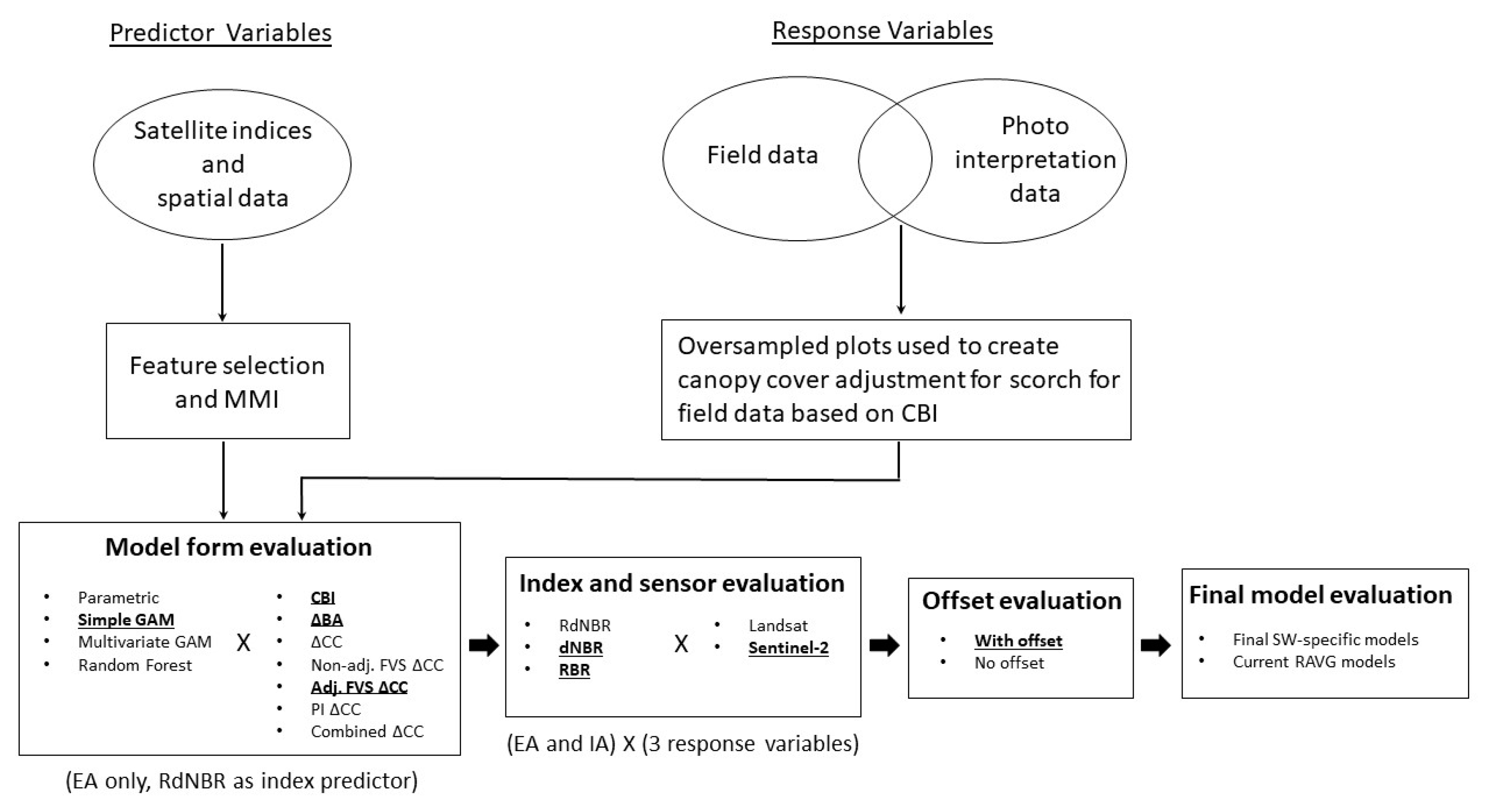
2.6. Model Development

To improve model accuracy based on anticipated difficulties in estimating burn severity in this region, we explored the use of additional variables and modeling methods beyond the current parametric models [17] used in RAVG fire severity and forest change products. Similar to previous studies, we included several variables derived from a 30 m DEM (U.S. Geological Survey, Reston, VA, USA) [39] shown to be relevant to burn severity, including elevation, slope, aspect, and topographic convergence index [31,40,41,42,43]. We evaluated non-parametric models because the utility of several of these algorithms has been demonstrated in the field of fire effects prediction, including random forest [40,41], boosted regression trees [42], and general additive models (GAM) [32]. Our response variables can be characterized as proportions which typically includes a mass of observations at 0 and 1 with continuous data between these bounds. Zero-and-one inflated data follow the beta (ZOIB) distribution [44], which we used in a GAM. We tested a variety of standard satellite indices that have been shown to predict burn severity and forest change, including RdNBR, dNBR, and RBR [12,13,16], and we tested each index with and without “offsets,” values calculated in unburned areas near each fire and intended to account for non-disturbance differences between the pre- and post-fire images. Given the high potential for monsoonal rains to occur quickly following fire, resulting in loss of ash cover, we did not use the conversion factor derived by Miller and Quayle (2015) [45] to modify 1-year post-fire models to produce immediate post-fire estimates for burn severity and stand change. Instead, we developed stand-alone models for immediate post-fire effects based on image pairs that used post-fire imagery captured immediately after the fire.

To predict burn severity, canopy cover change, and basal area change after wildfire, we developed and tested a series of parametric and non-parametric models, with data obtained from the Southwest. To limit the overall number of models evaluated, model form and different predictor variables were each evaluated in turn, rather than evaluating every permutation of model form and predictors (Figure 3). Only the best candidate models were carried forward into the next evaluation, i.e., once the model form was chosen, satellite indices were evaluated on only the selected model form. To compare candidate model performance, test mean squared error (MSE) was computed within a 7-fold cross validation and then averaged across folds. The details of the models sequentially tested are given in Appendix A.

The parametric models fit were of the form currently used in RAVG production (Craig Baker, pers. comm.), which are the inverse of those documented in Miller et al. (2009) [17] and follow a sine curve for ΔBA and ΔCC and natural log curve for CBI (Equations (1)–(3)). The application of these parametric models (Miller et al., 2009) [17] includes limits below and above which predictions are set to the minimum and maximum values, that is, zero and 100% loss, respectively, for ΔBA and ΔCC and zero and three, respectively, for CBI.

$$\mathrm{C}\mathrm{B}\mathrm{I}=\left(\frac{1}{c}\right)\ln \left(\frac{Index-a}{b}\right)$$

(1)

$$\mathsf{\Delta }\mathrm{B}\mathrm{A}=\sin \left(\frac{Index-a}{b}\right)$$

(2)

$$\mathsf{\Delta }\mathrm{C}\mathrm{C}=\sin \left(\frac{Index-a}{b}\right)$$

(3)

Index refers to any one of the satellite indices tested (dNBR, RdNBR, or RBR) and a, b, and c are constants.

3. Results

3.1. Model Development Process

Initial model development produced extensive results, which can be found in Appendix A and Appendix B. Models built from just the field-derived canopy cover datasets predicted better than those using combined canopy cover data (field- and PI-derived), so only the field-derived canopy cover response variable was carried forward. General additive models (GAMs) performed best as a group and were the model form carried forward into final model development. Multivariate GAMs were evaluated, but due to mixed results and the complexity of acquiring additional variables in the production phase, we elected to only carry forward simple GAMs into the final models (

Table A3. Comparison of test MSE (and standard deviation of test MSE in parentheses) averaged across 7 folds for each model form (parametric (Equations 1–3), simple GAM, multivariate GAM, and Random Forest) using EA Landsat RdNBR with offset as a predictor.

	Parametric	Simple GAM	Multivariate GAM	Random Forest
CBI	0.2486(0.0289)	0.0273(0.0032)	0.0267(0.0033)	0.2657(0.0247)
ΔBA	0.0504(0.0085)	0.0483(0.0104)	0.0473(0.0101)	0.0518(0.0040)
Non-adj. FVS ΔCC	0.0511(0.0081)	0.0484(0.0102)	0.0474(0.0094)	0.0518(0.0040)
Adj. FVS ΔCC	0.0392(0.0065)	0.0397(0.0072)	0.0390(0.0070)	0.0440(0.0048)
PI ΔCC	0.0514(0.0028)	0.0523(0.0035)	0.0530(0.0038)	0.0607(0.0050)
Combined ΔCC	0.0457(0.0015)	0.0481(0.0041)	0.0724(0.0032)	0.0492(0.0027)

Non-adj. FVS ΔCC is FVS-derived canopy cover change not adjusted for scorch. Adj. FVS ΔCC is scorch-adjusted FVS canopy cover change. PI ΔCC is the canopy cover change derived from the PI dataset. Combined ΔCC is canopy cover change derived from the combined scorch-adjusted FVS as well as PI canopy cover change.

). Indices derived from Sentinel data performed better than indices derived from LANDSAT data. The indices that performed best and which were carried forward into final model development were the RBR for the EA time series and dNBR for the IA (

Table A6. Test MSE (and standard deviation of test MSE in parentheses) averaged across 7-fold CV of single-predictor GAM models for the EA time series.

	RdNBR		dNBR		RBR
	Landsat	Sentinel-2	Landsat	Sentinel-2	Landsat	Sentinel-2
CBI	0.0273 (0.0032)	0.0275 (0.0033)	0.0260 (0.0021)	0.0256 (0.0018)	0.0244 (0.0020)	0.0240 (0.0018)
ΔBA	0.0483 (0.0104)	0.0455 (0.0087)	0.0495 (0.0062)	0.0465 (0.0052)	0.0450 (0.0070)	0.0416 (0.0059)
Adj. FVS ΔCC	0.0397 (0.0072)	0.0363 (0.0056)	0.0412 (0.0042)	0.0378 (0.0032)	0.0378 (0.0048)	0.0340 (0.0039)

and

Table A7. Test MSE (and standard deviation of test MSE in parentheses) averaged across 7-fold CV of single-predictor GAM models for the IA time series.

	RdNBR		dNBR		RBR
	Landsat	Sentinel-2	Landsat	Sentinel-2	Landsat	Sentinel-2
CBI	0.0333 (0.0022)	0.0273 (0.0018)	0.0215 (0.0021)	0.0185 (0.0020)	0.0227 (0.0021)	0.0193 (0.0021)
ΔBA	0.0710 (0.0092)	0.0642 (0.0103)	0.0440 (0.0052)	0.0416 (0.0069)	0.0454 (0.0057)	0.0424 (0.0079)
Adj. FVS ΔCC	0.0605 (0.0060)	0.0524 (0.0065)	0.0377 (0.0031)	0.0351 (0.0045)	0.0399 (0.0034)	0.0360 (0.0056)

). Indices with the offset used in calculations generally performed the best, so all final models were built using indices with the offset included (

Table A8. Test MSE (and standard deviation of test MSE in parentheses) for candidate models with and without offset.

	Sentinel-2 IA dNBR		Sentinel-2 EA RBR
	With Offset	No Offset	With Offset	No Offset
CBI	0.0185 (0.0020)	0.0193 (0.0018)	0.0240 (0.0018)	0.0253 (0.0019)
ΔBA	0.0416 (0.0069)	0.0428 (0.0065)	0.0416 (0.0059)	0.0443 (0.0064)
Adj. FVS ΔCC	0.0351 (0.0045)	0.03670 (0.0041)	0.0340 (0.0039)	0.0368 (0.0042)

).

3.2. Final Models

We compared the best candidate models (simple GAMs) to those used in the current RAVG products as of this writing [17]. The models built from Southwest data all had a lower test MSE than the current RAVG models [17] when applied to the Southwest data, suggesting that the Southwest models perform better when viewed as continuous data products. However, the results for accuracy and Kappa, which are used to evaluate categorical data response, were mixed (

Table 5. Comparison of our final SW models predicting CBI, ΔBA, and ΔCC (percent accuracy, Kappa, and test MSE) to models currently used in RAVG burn severity and forest change products at the time of this writing [17].

	IA SW-Specific Model (Sentinel-2 dNBR)			IA Current Model (Landsat RdNBR)			EA SW-Specific Model (Sentinel-2 RBR)			EA Current Model (Landsat RdNBR)
	Acc.	Kappa	Test MSE	Acc.	Kappa	Test MSE	Acc.	Kappa	Test MSE	Acc.	Kappa	Test MSE
CBI	61.4	46.7	0.0184	46.9	32.1	0.8753	62.0	47.0	0.0237	50.1	35.9	1.1265
ΔBA	52.2	33.9	0.0409	67.4	47.5	0.0547	56.1	38.1	0.0407	63.8	46.9	0.0705
ΔCC	50.7	38.0	0.0347	54.9	41.5	0.0886	53.4	41.2	0.0337	54.9	41.4	0.0518

). For CBI, all three metrics (test MSE, accuracy, and Kappa) suggested that the models built from Southwest data perform better in the Southwest. Conversely, the Miller et al. (2009) [17] canopy cover change models had higher accuracies and Kappa, though differences were mostly small. Likewise, for ΔBA the current RAVG [17] models had higher accuracy and Kappa (Table 5). However, for BA change for both EA and IA timeframes, several datapoints in the highest burn severity categories were predicted into the lowest burn severity category and vice versa with the current RAVG models [17] (

Table A9. Confusion matrix for Southwest model predicting IA CBI with Sentinel-2 dNBR with offset.

	Reference
Prediction	0–<0.1	0.1–<1.25	1.25–<2.25	2.25–3	Total	User’s Accuracy (%)
0–<0.1	9	3	0	0	12	75.0
0.1–<1.25	52	73	16	1	142	51.4
1.25–<2.25	1	29	67	24	121	55.4
2.25–3	0	0	4	58	62	93.5
Total	62	105	87	83	337
Producer’s accuracy (%)	14.5	69.5	77.0	69.9		61.4

,

Table A10. Confusion matrix for current RAVG (Miller et al., 2009) model predicting IA CBI with Landsat RdNBR with offset.

	Reference
Prediction	0–<0.1	0.1–<1.25	1.25–<2.25	2.25–3	Total	User’s Accuracy (%)
0–<0.1	61	87	39	1	188	32.4
0.1–<1.25	1	5	9	3	18	27.8
1.25–<2.25	0	11	36	23	70	51.4
2.25–3	0	2	3	56	61	91.8
Total	62	105	87	83	337
Producer’s accuracy (%)	98.4	4.8	41.4	67.5		46.9

,

Table A11. Confusion matrix for Southwest model predicting IA BA change with Sentinel-2 dNBR with offset.

	Reference
Prediction	0–<10%	10–<25%	25–<50%	50–<75%	75–<90%	90–<100%	Total	User’s Accuracy (%)
0–<10%	118	13	2	1	0	0	134	88.1
10–<25%	50	9	3	2	0	4	68	13.2
25–<50%	17	9	12	11	5	3	57	21.1
50–<75%	0	6	3	2	1	14	26	7.7
75–<90%	0	0	0	2	2	12	16	12.5
90–<100%	0	0	0	1	2	33	36	91.7
Total	185	37	20	19	10	66	337
Producer’s accuracy (%)	63.8	24.3	60.0	10.5	20.0	50.0		52.2

,

Table A12. Confusion matrix for current (Miller et al., 2009) model predicting IA BA change with Landsat RdNBR with offset.

	Reference
Prediction	0–<10%	10–<25%	25–<50%	50–<75%	75–<90%	90–<100%	Total	User’s Accuracy (%)
0–<10%	167	21	9	2	0	2	201	83.1
10–<25%	10	2	4	1	1	3	21	9.5
25–<50%	3	6	3	6	3	3	24	12.5
50–<75%	2	3	1	5	3	4	18	27.8
75–<90%	0	5	2	1	0	4	12	0.0
90–<100%	3	0	1	4	3	50	61	82.0
Total	185	37	20	19	10	66	337
Producer’s accuracy (%)	90.3	5.4	15.0	26.3	0.0	75.8		67.4

,

Table A13. Confusion matrix for Southwest model predicting IA scorch-adjusted canopy cover change with Sentinel-2 dNBR with offset.

	Reference
Prediction	0–<10%	10–<25%	25–<50%	50–<75%	75–<90%	90–<100%	Total	User’s Accuracy (%)
0–<10%	69	13	4	0	0	0	86	80.2
10–<25%	26	23	16	3	0	0	68	33.8
25–<50%	8	27	31	7	4	8	85	36.5
50–<75%	0	4	10	2	3	8	27	7.4
75–<90%	0	1	4	3	1	12	21	4.8
90–<100%	0	0	0	1	4	45	50	90.0
Total	103	68	65	16	12	73	337
Producer’s accuracy (%)	67.0	33.8	47.7	12.5	8.3	61.6		50.7

,

Table A14. Confusion matrix for current (Miller et al., 2009) model predicting IA canopy cover change with Landsat RdNBR with offset.

	Reference
Prediction	0–<10%	10–<25%	25–<50%	50–<75%	75–<90%	90–<100%	Total	User’s Accuracy (%)
0–<10%	98	40	15	1	0	0	154	63.6
10–<25%	1	8	8	3	0	1	21	38.1
25–<50%	2	10	15	2	0	2	31	48.4
50–<75%	2	4	13	3	2	8	32	9.4
75–<90%	0	1	5	5	3	4	18	16.7
90–<100%	0	5	9	2	7	58	81	71.6
Total	103	68	65	16	12	73	337
Producer’s accuracy (%)	95.1	11.8	23.1	18.8	25.0	79.5		54.9

,

Table A15. Confusion matrix for Southwest model predicting EA CBI with Sentinel-2 RBR with offset.

	Reference
Prediction	0–<0.1	0.1–<1.25	1.25–<2.25	2.25–3	Total	User’s Accuracy (%)
0–<0.1	1	0	0	0	1	100
0.1–<1.25	61	87	26	1	175	49.7
1.25–<2.25	0	18	56	17	91	61.5
2.25–3	0	0	5	65	70	92.9
Total	62	105	87	83	337
Producer’s accuracy (%)	1.6	82.9	64.4	78.3		62.0

,

Table A16. Confusion matrix for current (Miller et al., 2009) model prediction EA CBI with Landsat RdNBR with offset.

	Reference
Prediction	0–<0.1	0.1–<1.25	1.25–<2.25	2.25–3	Total	User’s Accuracy (%)
0–<0.1	60	83	28	1	172	34.9
0.1–<1.25	2	8	15	2	27	29.6
1.25–<2.25	0	10	37	16	63	58.7
2.25–3	0	4	7	64	75	85.3
Total	62	105	87	83	337
Producer’s accuracy (%)	96.8	7.6	42.5	77.1		50.1

and

Table A17. Confusion matrix for Southwest model predicting EA BA change with Sentinel-2 RBR with offset.

	Reference
Prediction	0–<10%	10–<25%	25–<50%	50–<75%	75–<90%	90–<100%	Total	User’s Accuracy (%)
0–<10%	131	13	1	0	0	0	145	90.3
10–<25%	39	7	5	2	0	4	57	12.3
25–<50%	12	11	10	6	5	4	48	20.8
50–<75%	3	3	3	8	0	14	31	25.8
75–<90%	0	3	1	1	3	14	22	13.6
90–<100%	0	0	0	2	2	30	34	88.2
Total	185	37	20	19	10	66	337
Producer’s accuracy (%)	70.8	18.9	50.0	42.1	30.0	45.5		56.1

). This does not diminish accuracy, but the magnitude of the error possible is higher than in the models built using the Southwest data. The model accuracy metric only factors in a binary response at each category and does not penalize differently for large versus small categorization errors. These results suggest that the ΔBA and ΔCC models built from Southwest data predict better as continuous products for the Southwest, but current RAVG models [17] predict the most observations in the correct categories.

4. Discussion

Our objective was to create and explore the efficacy of region-specific models for the southwest U.S. predicting burn severity and forest change with fire. Surprisingly, we found that current RAVG models are better categorical predictors for forest change than our region-specific models, although our models appear to serve as better continuous prediction tools. Our methods (Appendix A) and publicly available code (https://github.com/alreiner/SW_RAVG.git) (accessed on 1 August 2022) provide for the development of similar region-specific models in other systems.

4.1. Efficacy of Region-Specific Models in Assessing Post-Wildfire Change

We assessed the performance of region-specific fire effects models with test metrics for assessing the model’s ability to fit a continuous response or categorize the response. Categorical prediction is best assessed with the confusion matrix and accuracy, whereas test MSE is a metric more suitable for evaluating a continuous response. In general, the Miller et al. (2009) [17] ΔBA and ΔCC models may have better categorical prediction capabilities than models developed from the SW data; however, continuous and overall predictions from the Southwest models are superior when applied to Southwest data (Table 5). When the total vegetation cover is low in a spectral image, changes to the vegetation have lower impact on the spectral image, which could make for a weaker relationship between the indices and fire effects. Effectively, the sparser vegetation has the effect of increasing the substrate signal, which influences the indices. A wide variety of forested vegetation types are present in the Southwest and in our dataset, ranging from pinyon–juniper woodland to mixed conifer forest. The variation in the spectral signature may be wider than that of Miller et al. (2009) [17], which did not include arid woodlands.

Nuances between satellite indices factor into why various indices performed better in Southwest models. Cansler and McKenzie (2012) [46] note that in areas with little variation in pre-fire reflectance, meaning homogenous vegetation cover, dNBR has little advantage over RdNBR. Parks et al. (2014) [15] note that areas with very low pre-fire NBR can cause very high or very low RdNBR due to the square root in the denominator, leading RBR to potentially perform better. The Southwest has highly variable canopy cover and many vegetation types with low cover, so it is not surprising that RBR proved optimal in some instances. A few factors could explain why dNBR was the best IA predictor, whereas RBR was the best EA predictor. Parks et al. (2014) [15] note that dNBR is correlated to pre-fire NBR. Severity is understandably correlated to pre-fire vegetation cover in the Southwest, as stand-replacing fire regimes occur in the highest elevation sites dominated by mesic forests, which inherently have high vegetation cover compared to the arid woodlands of the low elevations. For the IA time series, this correlation would likely boost the predictive capacity of a satellite index. However, for the EA time series, derived one growing season after the fire, giving the understory more time to recover, RBR, an index normalized by pre-fire vegetation cover, was favored, suggesting that normalizing the index to pre-fire vegetation cover is more useful for modeling at that timeframe. This normalization makes finer differences in dNBR more apparent in the lower-cover portions of the study area, which likely had more understory recovery than the closed-canopy forest types. The Sentinel-2-based indices may have performed better than the Landsat indices partially due to the finer scale (20 m rather than 30 m) [47].

The zero-and-one inflated beta distribution [44] is suitable where a binary response is a frequent outcome in an otherwise continuous data distribution. In the context of fire severity, ΔCC, and ΔBA, these are unburned plots or plots with 100% canopy scorch. Accounting for this distribution in a GAM may have given the GAM models an advantage over the parametric and random forest models by better addressing the binary nature of the data. The Southwest GAM models generally outperformed the Southwest parametric models. It is plausible that GAMs using a zero-and-one inflated beta distribution derived with the Miller et al. (2009) [17] data might predict with greater accuracy.

In our analyses, multivariate GAM performance may have been reduced by several factors. The stepwise procedure we utilized for multivariate model development is reliant on appropriate selection of plausible a priori variables with potential collinearity between variables. For this reason, it can be sensitive to over-fitting if care is not taken when selecting a priori variables [48]. However, we used a limited selection of a priori variables and selected only those with sufficiently high importance. The gamlss package available in R allows the use of the zero-and-one inflated beta distribution; however, it does not incorporate model selection algorithms utilizing shrinkage such as LASSO. The shrinkage algorithms would be more effective at reducing the moderate to low importance predictors to zero. In our analyses, the relationships of the non-satellite predictors were weak, so there was little additional information to be added from each. Holden et al. (2009) [40] noted that topographic variables which describe moisture availability present shifting, and perhaps conflicting, roles with increasing elevation. For example, at lower elevations, aspect can influence vegetation distributions and fuel loads due to changes in moisture availability. It is possible that at lower elevations, only northerly aspects have enough moisture and fuels to burn with high severity. Conversely, at higher elevation where mixed conifer forests are dominant, southerly aspects or areas that experience lower moisture have adequate fuels to burn with high severity and could be more likely to do so given the lower fuel moistures. These differences in the way aspect and other geomorphic predictor variables relate to severity with increasing elevation may be important for process-based modeling but are less useful for multivariate GAMs. Models produced from larger datasets and machine learning methods capable of incorporating complex interactions may capture these interconnections better.

4.2. Influence of Forest Change Measurements on Error

Field measurements and photo interpretation methods each have an irreducible error when estimating canopy cover, which can weaken canopy cover models. Error in field methods can arise from measurement or sampling error, and error can be introduced in photo interpretation due to shadows or edges being less interpretable. Field plots were intentionally located in areas of relatively homogenous severity [17], whereas PI plots were located on a systematic grid, which could have increased the ratio of PI plots in areas of mixed severity, potentially muting the CBI to satellite index relationship.

Changes in canopy cover and tree mortality in areas of heterogeneous severity would have a weaker relationship between predictor and response variables. This may have led to the PI models having weaker relationships with satellite indices when compared to the field plots. Background mortality may also be a confounding error source in photo interpretation where pre-fire photos were taken several years before the fire and some background mortality would be expected even in the absence of fire. Similarly, in this analysis, the post-fire aerial resource photography utilized was collected the same year as the fire, which would not pick up delayed mortality for the EA timeframe. Field data were collected the year after fire, so include the 1-year delayed mortality with the assumption of EA mortality being the same as IA, which may not be entirely accurate but is likely a minor error considering overall error sources and precision of the data and models.

4.3. Implications and Directions for Future Research

The implications of this research support continued development of the synergy between remotely sensed data and machine learning methods as well as appraisal of current models and development of improved or region-specific models. With the increasing variety of remotely sensed data as well as machine learning methods with which to develop models, more nuance is possible in fire effects modeling. New sensors are being developed each year, expanding the capacity for remote data collection, and data post-processing methods as well as machine learning algorithms are continually being expanded and improved. New sensors and machine learning will aid in more precise and accurate model development in the years to come. Automated workflows could improve the use of these data and machine learning methods. The improvements and lessons our Southwest models offer include addressing the zero-and-one inflated beta distribution inherently with the choice of model form and algorithm. A drawback to the parametric models currently used in RAVG products is the need to apply limits to the sine and natural log functions at points of inflection or nonsensical predictions, capping them at minimum and maximum predictions. These limits affect the categorization of a portion of the data range, which can influence categorization errors. Our Southwestern-specific models and approach to other arid or semi-arid regions, such as the southwestern Rockies and the Great Basin, may improve fire effects modeling and provide better information to researchers and managers under increasingly variable fire regimes.

Future research could benefit from three tactics not employed in this project: using the individual bands from the remote satellite sensors rather than indices, exploring additional machine learning methods other than GAM with modifications to accommodate the zero-and-one inflated distribution, and employing composite images through Google Earth Engine (GEE). Indices are useful in that they compile information from several relevant variables into one variable, making models, relationships, and predictions easier to understand. However, there is some information loss when multiple variables are combined into an index. Applying multivariate and machine learning modeling methods to the variables addressed in this research plus the individual band differences or individual bands such as pre- and post-fire bands five and seven and NBR may provide additional predictive power [49]. Additional variables not used in this study could improve model results, namely active fire data such as those derived from MODIS and VIIRS [50,51]. This concept could be taken a step further by exploring linear unmixing, in which the entire spectrum of image information is used rather than categorizing the image data into bands [52]. The gamlss package in R is one of the few ready-made algorithms available to model the binary and continuous response of a dataset simultaneously. It is possible to split data into binary and continuous response subsets and model them separately; however, as the split is non-random, these models will be applied to data on which they were not developed, which results in sample selection bias. Methods and algorithms to overcome this bias are being developed and should be explored to allow a variety of proven machine learning methods beyond GAM to be applied. Previous studies [42] have used the GEE environment to create composite images from collections of imagery based on date and quality constraints, from which more robust models can be developed as these data moderate differences in individual images. Given that we focused on exploring Sentinel-2 data just as data from this sensor were becoming available, we did not have a broad history from which to pull multiple images for the 2017 fires sampled, so we opted not to pursue the use of composite images. However, others have found value in this approach [42], which warrants future exploration.

Appropriately designed field training data are key building blocks to creating improved or regional models. Although CBI has historically been utilized as the primary response variable in burn severity models, there is value in collecting and modeling as response variables other more mechanistically linked or forest structure data rather than unitless and subjective data such as CBI [50,53]. Additionally, field verification of new and existing models could help to highlight areas where revision to current models would be beneficial. Archiving data and methods would greatly facilitate re-analysis of historical datasets with more contemporary statistical learning tools as well as meta-analyses using combined data or the use of similar datasets as validation sets for model development.

5. Conclusions

Our region-specific post-wildfire model had several advantages over conventional California-based models and showcases the utility of developing region-specific models. However, measurement error, limitations to current statistical packages, and the complexity of untangling the remote-sensing data spectrum are among the potential issues with developing and implementing similar models to assess post-wildfire change. Continued development, collection, and archival of remote and ground-based data will provide for better calibration and more accurate decision making. Our success in improving on the Miller (2009) [17] models should provide guidance for future region-specific adaptations of these models.

References

1. National Interagency Coordination Center. Wildland Fire Summary and Statistics Annual Report 2021. 2021. Available online: https://www.predictiveservices.nifc.gov/intelligence/2021_statssumm/annual_report_2021.pdf (accessed on 24 August 2022).
2. Swetnam, T.W.; Baisan, C.H. Historical fire regime patterns in the southwestern United States since AD 1700. In Fire Effects in Southwestern Forest: Proceedings of the 2nd La Mesa Fire Symposium, Los Alamos, NM, USA, 29–31 March 1994; Allen, C.D., Ed.; USDA Forest Service General Technical Report RM-GTR-286; RMRS: Fort Collins, CO, USA, 1996; pp. 11–32. [Google Scholar]
3. Swetnam, T.W.; Brown, P.M. Climatic inferences from dendroecological reconstructions. In Dendroclimatology; Hughes, M., Swetnam, T., Diaz, H., Eds.; Developments in Paleoenvironmental Research; Springer: Berlin/Heidelberg, Germany, 2011; Volume 11. [Google Scholar]
4. Hurteau, M.D.; Bradford, J.B.; Fule, P.Z.; Taylor, A.H.; Martin, K.L. Climate change, fire management, and ecological services in the southwestern U.S. For. Ecol. Manag. 2014, 327, 280–289. [Google Scholar] [CrossRef]
5. Stefanidis, S.; Alexandridis, V.; Spalevic, V.; Mincato, R.L. Wildfire Effects on Soil Erosion Dynamics: The Case of 2021 Megafires in Greece. Agric. For. 2022, 68, 49–63. [Google Scholar]
6. Wilder, B.J.; Lancaster, J.T.; Cafferata, P.H.; Coe, D.B.; Swanson, B.J.; Lindsay, D.N.; Short, W.R.; Kinoshita, A.M. An analytical solution for rapidly predicting post-fire peak streamflow for small watersheds in southern California. Hydrol. Process. 2021, 35, e13976. [Google Scholar] [CrossRef]
7. Morgan, P.; Keane, R.E.; Dillon, G.K.; Jain, T.B.; Hudak, A.T.; Karau, E.C.; Sikkink, P.G.; Holden, Z.A.; Strand, E.K. Challenges of assessing fire and burn severity using field measures, remote sensing and modelling. Int. J. Wildland Fire 2014, 23, 1045. [Google Scholar] [CrossRef]
8. Agee, J.K. Fire Ecology of Pacific Northwest Forests; Island Press: Washington, DC, USA, 1993. [Google Scholar]
9. Lentile, L.B.; Smith, F.W.; Shepperd, W.D. Influence of topography and forest structure on patterns of mixed severity fire in ponderosa pine forests of the South Dakota Black Hills, USA. Int. J. Wildland Fire 2006, 15, 557–566. [Google Scholar] [CrossRef]
10. Dillon, G.K.; Panunto, M.F.; Davis, B.; Morgan, P.; Birch, D.S.; Jolly, W.M. Development of a Severe Fire Potential Map for the Contiguous United States; General Technical Report RMRS-GTR-415; U.S. Department of Agriculture, Forest Service, Rocky Mountain Research Station: Fort Collins, CO, USA, 2020; 107p. [Google Scholar]
11. Miesel, J.; Reiner, A.; Ewell, C.; Maestrini, B.; Dickinson, M. Quantifying changes in total and pyrogenic Carbon stocks across burn severity gradients using active wildland fire incidents. Front. Earth Sci. 2018, 6, 41. [Google Scholar] [CrossRef]
12. Key, C.H.; Benson, N.C. 2006. Landscape Assessment: Sampling and Analysis Methods. In FIREMON: Fire Effects Monitoring and Inventory System; Lutes, D.C., Keane, R.E., Caratti, J.F., Key, C.H., Benson, N.C., Sutherland, S., Gangi, L.J., Eds.; USDA Forest Service General Technical Report RMRS-GTR-164-CD; RMRS: Ogden, UT, USA; p. LA 1–51.
13. Miller, J.D.; Thode, A.E. Quantifying burn severity in a heterogeneous landscape with a relative version of the delta Normalized Burn Ratio (dNBR). Remote Sens. Environ. 2007, 109, 66–80. [Google Scholar] [CrossRef]
14. Key, C.H. Ecological and sampling constraints on defining landscape burn severity. Fire Ecol. 2006, 2, 34–59. [Google Scholar] [CrossRef]
15. Parks, S.A. Mapping day-of-burning with coarse-resolution satellite fire-detection data. Int. J. Wildland Fire 2014, 23, 215–223. [Google Scholar] [CrossRef]
16. Parks, S.A.; Holsinger, L.M.; Voss, M.A.; Loehman, R.A.; Robinson, N.P. Mean composite fire severity metrics computed with Google Earth Engine offer improved accuracy and expanded mapping potential. Remote Sens. 2018, 10, 879. [Google Scholar] [CrossRef]
17. Miller, J.D.; Knapp, E.E.; Key, C.H.; Skinner, C.N.; Isbell, C.J.; Creasy, R.M.; Sherlock, J.W. Calibration and validation of the relative differenced Normalized Burn Ratio (RdNBR) to three measures of fire severity in the Sierra Nevada and Klamath Mountains, California, USA. Remote Sens. Environ. 2009, 113, 645–656. [Google Scholar] [CrossRef]
18. Kolden, C.A.; Smith, A.M.S.; Abatzoglou, J.T. Limitations and utilisation of Monitoring Trends in Burn Severity products for assessing wildfire severity in the USA. Int. J. Wildland Fire 2015, 24, 1023–1028. [Google Scholar] [CrossRef]
19. Huffman, D.W.; Zegler, T.J.; Fule, P.Z. Fire history of a mixed conifer forest on the Mogollon Rim, northern Arizona, USA. Int. J. Wildland Fire 2015, 24, 680–689. [Google Scholar] [CrossRef]
20. O’Connor, C.D.; Falk, D.A.; Lynch, A.M.; Swetnam, T.W. Fire severity, size and climatic associations diverge from historical precedent along an ecological gradient in the Pinaleño Mountains, Arizona, USA. Int. J. Wildland Fire 2014, 329, 264–278. [Google Scholar]
21. Miller, J.D.; Skinner, C.; Safford, H.D.; Knapp, E.E.; Ramirez, C.M. Trends and causes of severity, size, and number of fires in northwestern California, USA. Ecol. Appl. 2012, 22, 184–203. [Google Scholar] [CrossRef]
22. Sheppard, P.R.; Comrie, A.C.; Packin, G.D.; Angersbach, K.; Hughes, M.K. The climate of the US southwest. Clim. Res. 2002, 21, 219–238. [Google Scholar] [CrossRef]
23. Alexandrov, G.A.; Ames, D.; Bellocchi, G.; Bruen, M.; Crout, N.; Erechtchoukova, M.; Hildebrandt, A.; Hoffman, F.; Jackisch, C.; Khaiter, P.; et al. Technical assessment and evaluation of environmental models and software: Letter to the Editor. Environ. Model. Softw. 2011, 26, 328–336. [Google Scholar] [CrossRef]
24. Saberi, J.S. Quantifying Burn Severity in Forests of the Interior Pacific Northwest: From Field Measurements to Satellite Spectral Indices. Master’s Thesis, University of Washington, Seattle, WA, USA, 2019. [Google Scholar]
25. Flora of North America Editorial Committee (Ed.) Flora of North America North of Mexico; Flora of North America Editorial Committee: New York, NY, USA; Oxford, MI, USA, 1993; Volume 22, Available online: http://beta.floranorthamerica.org (accessed on 1 May 2021).
26. Schrader, D.K.; Min, B.C.; Matson, E.T.; Dietz, J.E. Real-time averaging of position data from multiple GPS receivers. Measurement 2016, 90, 329–337. [Google Scholar] [CrossRef]
27. Parks, S.A.; Holsinger, L.M.; Koontz, M.J.; Collins, L.; Whitman, E.; Parisien, M.; Loehman, R.A.; Barnes, J.L.; Bourdon, J.F.; Boucher, J.; et al. Giving ecological meaning to satellite-derived fire severity metrics across North American forests. Remote Sens. 2019, 11, 1735. [Google Scholar] [CrossRef]
28. Harvey, B.J.; Donato, D.C.; Romme, W.H.; Turner, M.G. Influence of recent bark beetle outbreak on burn severity and postfire tree regeneration in Montane Douglas-fir forests. Ecology 2013, 94, 2475–2486. [Google Scholar] [CrossRef]
29. Forest Vegetation Simulator (FVS) Software, 2019.11.01 version. Available online: https://www.fs.usda.gov/fvs/index.shtml (accessed on 16 September 2019).
30. Dixon, G.E. Essential FVS: A User’s Guide to the Forest Vegetation Simulator; Internal Report; Department of Agriculture, Forest Service: Fort Collings, CO, USA, 2002. [Google Scholar]
31. Harvey, B.J.; Andrus, R.A.; Anderson, R.A. Incorporating biophysical gradients and uncertainty into burn severity maps in a temperate fire-prone forested region. Ecosphere 2019, 10, e02600. [Google Scholar] [CrossRef]
32. Crookston, N.L.; Stage, A.R. Percent Canopy Cover and Stand Structure Statistics from the Forest Vegetation Simulator; General Technical Report, RMRS-GTR-24; Department of Agriculture, Forest Service, Rocky Mountain Research Station: Ogden, UT, USA, 1999; 15p. [Google Scholar]
33. Jenkins, J.C.; Chojnacky, D.C.; Heath, L.S.; Birdsey, R.A. National-scale biomass estimators for United States tree species. For. Sci. 2003, 49, 12–35. [Google Scholar]
34. Christopher, T.A.; Goodburn, J.M. The effects of spatial patterns on the accuracy of Forest Vegetation Simulator (FVS) estimates of forest canopy cover. West. J. Appl. For. 2008, 23, 5–11. [Google Scholar] [CrossRef] [Green Version]
35. Copernicus Sentinel Data; Retrieved from ASF DAAC [April 2019]; ESA: Paris, France, 2019.
36. Coulston, J.W.; Moisen, G.G.; Wilson, B.T.; Finco, M.V.; Cohen, W.B.; Brewer, C.K. Modeling Percent Tree Canopy Cover: A Pilot Study. Photogramm. Eng. Remote Sens. 2012, 78, 715–727. [Google Scholar] [CrossRef]
37. Toney, C.; Liknes, G.; Lister, A.; Meneguzzo, D. Assessing alternative measures of tree canopy cover: Photo-interpreted NAIP and ground-based estimates. In Monitoring Across Borders: 2010 Joint Meeting of the Forest Inventory and Analysis (FIA) Symposium and the Southern Mensurationists; McWilliams, W., Roesch, F.A., Eds.; e-General Technical Report SRS-157; U.S. Department of Agriculture, Forest Service, Southern Research Station: Asheville, NC, USA, 2012; pp. 209–215. [Google Scholar]
38. Falkowski, M.J.; Evans, J.S.; Naugle, D.E.; Hagen, C.A.; Carleton, S.A.; Maestas, J.D.; Khalyani, A.H.; Poznanovic, A.J.; Lawrence, A.J. Mapping tree canopy cover in support of proactive Prairie Grouse conservation in western North America. Rangel. Ecol. Manag. 2017, 70, 15–24. [Google Scholar] [CrossRef]
39. U.S. Geological Survey. USGS 30 Meter Resolution, One-Sixtieth Degree National Elevation Dataset for CONUS, Alaska, Hawaii, Puerto Rico, and the U.S. Virgin Island; U.S. Geological Survey: Reston, VA, USA, 1999. [Google Scholar]
40. Holden, Z.; Morgan, P.; Evans, J.S. A predictive model of burn severity based on 20-year satellite-inferred burn severity data in a large southwestern US wilderness area. For. Ecol. Manag. 2009, 258, 2399–2406. [Google Scholar] [CrossRef]
41. Dillon, G.K.; Holden, Z.A.; Morgan, P.; Crimmins, M.A.; Heyerdahl, E.K.; Luce, C.H. Both topography and climate affected forest and woodland burn severity in two regions of the western US, 1984 to 2006. Ecosphere 2011, 2, 130. [Google Scholar] [CrossRef]
42. Parks, S.A.; Holsinger, L.M.; Panunto, M.H.; Jolly, W.M.; Dobrowski, S.Z.; Dillon, G.K. High-severity fire: Evaluating its key drivers and mapping its probability across western US forests. Environ. Res. Lett. 2018, 13, 044037. [Google Scholar] [CrossRef]
43. Dilts, T.E. Topography Tools for ArcGIS 10.1. University of Nevada Reno. 2015. Available online: http://www.arcgis.com/home/item.html?id=b13b3b40fa3c43d4a23a1a09c5fe96b9 (accessed on 16 September 2019).
44. Ospina, R.; Ferrari, S.L.P. A general class of zero-or-one inflated beta regression models. Comput. Stat. Data Anal. 2012, 56, 1609–1623. [Google Scholar] [CrossRef]
45. Miller, J.D.; Quayle, B. Calibration and validation of immediate post-fire satellite-derived data to three severity metrics. Fire Ecol. 2015, 11, 12–30. [Google Scholar] [CrossRef]
46. Cansler, A.C.; McKenzie, D. How robust are burn severity indices when applied in a new region? Evaluation of alternate field-based and remote-sensing methods. Remote Sens. 2012, 4, 456–483. [Google Scholar] [CrossRef]
47. Van Wagtendonk, J.; Root, R.R.; Key, C.K. Comparison of AVIRIS and Landsat ETM+ detection capabilities for bur severity. Remote Sens. Environ. 2004, 92, 397–408. [Google Scholar] [CrossRef]
48. Burnham, K.P.; Anderson, D.R. Model Selection and Multimodel Inference: A Practical Information-Theoretic Approach; Spring Science & Business Media: New York, NY, USA, 2002; 512p. [Google Scholar]
49. Smith, A.M.S.; Falkowski, M.J.; Hudak, A.T.; Evans, J.S.; Robinson, A.P.; Steele, C.M. A cross-comparison of field, spectral, and lidar estimates of forest canopy cover. Can. J. Remote Sens. 2009, 35, 447–459. [Google Scholar] [CrossRef]
50. McCarley, T.R.; Hudak, A.T.; Sparks, A.M.; Vaillant, N.M.; Meddens, A.J.H.; Trader, L.; Mauro, F.; Kreitler, J.; Boschetti, L. Estimating wildfire fuel consumption with multitemporal airborne laser scanning data and deomonstrating linkage with MODIS-derived fire radiative energy. Remote Sens. Environ. 2020, 251, 112114. [Google Scholar] [CrossRef]
51. Li, F.; Zhang, X.; Kondragunta, S.; Csiszar, E. Comparison of fire radiative power estimates from VIIRS and MODIS observations. J. Geophys. Res. Atmos. 2018, 123, 4545–4563. [Google Scholar] [CrossRef]
52. Lentile, L.B.; Holden, Z.A.; Smith, A.M.S.; Falkowski, M.J.; Hudak, A.T.; Morgan, P.; Lewis, S.A.; Gessler, P.E.; Benson, N.C. Remote sensing techniques to assess active fire characteristics and post-fire effects. Int. J. Wildland Fire 2006, 15, 319. [Google Scholar] [CrossRef]
53. Smith, A.M.S.; Sparks, A.M.; Kolden, C.A.; Abatzoglou, J.T.; Talhelm, A.F.; Johnson, D.M.; Boschetti, L.; Lutz, J.A.; Apostol, K.G.; Yedinak, K.M.; et al. Towards a new paradigm in fire severity research using dose-response experiments. Int. J. Wildland Fire 2016, 25, 158–166. [Google Scholar] [CrossRef]
54. Ferri, C.; Hernandez-Orallo, J.; Modroiu, R. An experimental comparison of performance measures for classification. Pattern Recognit. Lett. 2009, 30, 27–38. [Google Scholar] [CrossRef]
55. Cohen, J. A coefficient of agreement for nominal scales. Educ. Psychol. Meas. 1960, 20, 37–46. [Google Scholar] [CrossRef]
56. Chicco, D.; Jurman, G. The advantages of the Matthews correlation coefficient (MCC) over F1 score and accuracy in binary classification evaluation. BMC Genom. 2020, 21, 6. [Google Scholar] [CrossRef]
57. Delgado RTibau, X. Why Cohen’s Kappa should be avoided as a performance measure in classification. PLoS ONE 2019, 14, e0sss916. [Google Scholar] [CrossRef] [PubMed]
58. Welch, K.R.; Safford, H.D.; Young, T.P. Predicting conifer establishment post wildfire in mixed conifer forests of the North American Mediterranean-climate zone. Ecosphere 2016, 7, e01609. [Google Scholar] [CrossRef]
59. Kendall, M. A New Measure of Rank Correlation. Biometricka 1938, 30, 81–89. [Google Scholar] [CrossRef]
60. Wang, Y.; Li, Y.; Cao, H.; Xiong, M.; Shugart, Y.Y.; Jin, L. Efficient test for nonlinear dependence of two continuous variables. BMC Bioinform. 2015, 16, 260. [Google Scholar] [CrossRef]
61. Barton, K. MuMin: Multi-Model Inference. R Package. Version 4.0.5. Available online: https://cran.r-project.org/web/packages/MuMIn/index.html (accessed on 1 June 2020).
62. Breiman, L. Random Forests. Mach. Learn. 2001, 45, 5–23. [Google Scholar] [CrossRef] [Green Version]
63. R core Team. R: A Language and Environment for Statistical Computing; R Foundation for Statistical Computing: Vienna, Austria, 2020. [Google Scholar]
64. R Documentation. Gamlss.dist R Package (version 5.3-2). https://www.rdocumentation.org/packages/gamlss.dist/versions/5.3-2. (accessed on 1 May 2021). BEINF: The Beta Inflated Distribution for Fitting a GAMLSS. Available online: https://www.rdocumentation.org/packages/gamlss.dist/versions/6.0-5/topics/BEINF (accessed on 1 May 2021).
65. Stasinopoulos, M.; Rigby, B.; Voudouris, V.; Heller, G.; De Bastiani, F. Flexible Regression and Smoothing: The GAMLSS Packages in R. July 23, 2017; CRC Press: Boca Raton, FL, USA, 2017. [Google Scholar]
66. LANDFIRE Program. Available online: https://landfire.gov/cbd.php (accessed on 1 September 2019).
Figure 1. Locations of 2017 and 2018 fires where field plots were located.
Fire 05 00137 g001
Figure 2. A schematic of the area of adjacent 20 m pixels within a 30 m radius circle factored into the weighting of the kernel used to smooth Sentinel-2 data.
Fire 05 00137 g002
Figure 3. A flowchart of the analysis process. Circles indicate datasets and squares indicate analysis processes. Thin arrows depict where specific processed data are used; see Methods Section and Appendix A for complete description of all data used. Bold arrows indicate model evaluation steps taken in sequence. Variables and model form in bold and underlined were those carried forward into successive model development steps.
Fire 05 00137 g003