Article

Parametric Analysis of a Steel Frame under Fire Loading Using Monte Carlo Simulation

School of Mathematics, Computer Science and Engineering, City, University of London, London EC1V 0HB, UK
*
Author to whom correspondence should be addressed.
Submission received: 28 December 2021 / Revised: 7 February 2022 / Accepted: 9 February 2022 / Published: 14 February 2022
(This article belongs to the Special Issue Performance-Based Design in Structural Fire Engineering)

Abstract

:
In this paper, the parametric analysis of the thermal and structural response of a two-storey, single-zone steel frame building on fire is made considering different parameters Monte Carlo simulation is used to generate random variables for the opening factor, fire compartment area and finally the beam flange thickness. Using the random parameter generated, a sequential thermal and mechanical analysis was conducted using the finite element software ABAQUS. The first step was a heat transfer analysis, followed by mechanical analysis. The effect of different parameters on the thermal and mechanical response of the structure was studied.

1. Introduction

Steel has been the forefront of efficient construction in the last few years, where it has been used widely in the construction of high-rise buildings, industrial structures and residential structures. What makes steel one of the most appealing materials in the construction industry is its engineering properties. The most appealing properties of steel are its strength to weight ratio, ductility and flexibility. Such properties allow designers to build structures such as skyscrapers, which certainly would have not been possible with any other material. Steel can also be prefabricated and shipped to construction sites easily, which is quite beneficial when it comes to meeting the ever-increasing demands of new buildings. Nevertheless, there is a huge downside to using steel as a construction material because of its low resistance to fire when compared to other construction materials such as concrete. Steel loses almost half of its strength when subjected to temperature which is equal to or greater than 590 °C, which will eventually lead the structure to fail. The losses that follow structural failures caused by fire are colossal and can take different forms, such as loss of human lives, environmental loss and economical loss. Hence, the insurance of structural stability of a building under fire loading has been one of the most important and challenging aspects when it comes to designing a new structure [1]. It is important that in the event of a fire, structures are able to withstand the minimum level of life safety not only for the occupants but also fire fighters and the public that are in proximity of the building. The minimum level of fire safety design must ensure a reduction of the risk of deaths and injuries, protect the contents of a building, and ensure that the building continue to function after the fire with the least amount of repair possible.
In order to ensure that the structure meets the fire safety design objectives, designers have to follow one of two methods; the first is the prescriptive method, where a detailed description of the types and shapes of materials used in the design, the thickness of protection layer on structural elements and even the details of construction are given. However, this method relies solely on previous experience of the standard structural fire design tests. While this approach is very useful when it comes to static situations, it sometimes fails to meet the fire safety requirements of a building, raising concerns about the limitations of this method. One of its limitations is that the standard structural fire design tests assume that the structural elements of a building work independently, which is not the case in reality [2,3]. This approach is usually used for quick solutions and for junior designers, because it does not require an in-depth knowledge of the field.
The second method is the performance-based approach, which indicates how a structure will perform when subjected to different load conditions. Designers who use this method need to develop an accurate numerical simulation for fire loading to assess the fire safety resistance of the structure [4,5,6,7]. There are three main components to this approach: fire modelling, thermal analysis and structural analysis [2,3]. Keeping this in mind, this method allows designers to come up with solutions to build complex structures that were never possible with a standard prescriptive approach. This approach is usually adopted for more optimum solutions that require computational skills and deep understanding of the field.
There are a number of different modelling techniques commonly used today to predict the different fire scenarios instead of carrying out experimental tests. The techniques used range from simple hand calculations to more advanced computational techniques. Deciding which technique to use depends on the level of accuracy needed for the project, time restrictions and computational resources. With the development of software packages, designers can use a number of methods to predict possible fire scenarios in a building in order to further control the risk of a fire event. Some of these methods include zone models, computational fluid dynamics (CFD) [8] models and finite element (FE) models [9]. Zone models are simple computational models that operate on the basis of dividing a compartment area into separate zones, with the assumption that the temperature condition is uniform throughout each zone. CFD models are more sophisticated than zone models, because they analyze the fluid flow and heat transfer by solving the fundamental equations of fluid dynamics. Finally, FE models operate by dividing a large geometry into several hundred smaller parts that interact with each other. Given the different methods designers can adopt to predict the different fire scenarios, the uncertain nature of the different factors affecting a fire event the structural stability of a building one of the most challenging responsibilities for structural engineers. The fuel, load density and ventilation areas are all factors that contribute to a fire event and its duration. Moreover, the unpredictable nature of the response of structural elements to fire makes the whole fire process stochastic. As a result, the engineering design of structural fire is either based on empirical studies of the behavior of fire or on reliability analysis [10].
The FE modelling technique is one of the most straightforward methods used to predict the thermal and structural behavior of the structural members, according to [4,5,6,7]. The simulation works by breaking up large geometry to hundreds of smaller and simpler parts that interact together. In order to run the simulation using the finite element modelling technique, the thermal and mechanical properties of the material used in construction have to be calculated according to design codes. Design codes such as Eurocode provide formulas to calculate the thermal properties of a material and curves to obtain gas temperatures. The values obtained from the formulas provided can then be applied directly to the model using software packages.
However, most variables used during the fire analysis are either estimated or assumed, which makes the efficiency of the design in doubt and highlights the importance of the concept of intensive parametric study in structural fire design. As in reality, the parameters vary due to different fire scenarios; to effectively study the influence of different parameters, one of the promising methods is the Monte Carlo simulation [11]. This method generates hundreds of random variables for the different stochastic parameters that relate to fire, which allow designers to analyze the buildings under different fire scenarios, and thus to maximize the reliability and safety of the design.
Therefore, in this paper, the parametric analysis of the thermal and structural response of a two-story, single-zone steel frame building to fire is made considering different parameters; Monte Carlo simulation is used to generate random variables for the opening factor, fire compartment area and the beam flange thickness. Using the random parameters generated, a sequential thermal and mechanical analysis was conducted using the finite element software ABAQUS. The first step was a non-linear heat transfer analysis, followed by a non-linear mechanical analysis. The effect of different parameters on the thermal and mechanical response of the structure was studied.

2. Monte Carlo Simulation

The Monte Carlo Simulation is used here to generate the random parameters which will affect the fire scenarios and the thermal response of the structural steel members in a steel framed building. The key factors affecting the fire scenarios and thermal response of a structure under fire conditions are explained here

2.1. Time-Temperature Curves for a Compartment

The room temperature of a building in fire can be calculated using the formulas from Eurocode, BS EN 1993-1-2: Eurocode 1 part 1.2 [12] which gives the parametric time temperature of a compartment in fire:
θ g = 20 + 1325   ( 1 0.324   e 0.2 t * 0.204 e 1.7 t * 0.472 e 19 t * )
With
t* = t × Γ
Γ = [O/b]2/(0.04/1160)2
O = A v   h e q / A t
b = ( ρ c λ )
where θ g   is the gas temperature in the fire compartment (°C), t is the time (m), O is the opening factor (m1/2), b is the thermal diffusivity (J/m2 s1/2 K), ρ is the density (kg/m3), C is the specific heat (J/kgK), λ is the thermal conductivity (W/mK), At is the total internal surface area of the compartment (m2), Av is the area of ventilation (m2) and heq is the height of openings (m) [12,13].

2.2. Thermal Response of Structural Members

For unprotected steel sections, the increase of temperature in a small time interval is given by BS EN 1993-1-2: Eurocode 3 [13] as follows:
Δ θ a , t = k s h A m / V c a ρ a h ˙ n e t Δ t
where, Δ θ a , t is the increase of temperature. A m / V is the section factor for unprotected steel member. A m is the exposed surface area of the member per unit length. V is the volume if the member per unit length. c a is the specific heat of steel. ρ a is density of the steel.

2.3. Monte Carlo Simulation

Based on above formulas from the design code, three main parameters dominate the room temperature and thermal response of the structural member. They are the opening factor (O), the compartment area (Acom) and the cross-sectional area of the structural members (Am). Therefore, in the Monte Carlo simulation, the opening factor (O), the compartment area (Acom) and the thickness of the flange for the steel I-section beam were selected as the key parameters for the random simulation. These three parameters were selected based on Equations (1) and (3), since these three parameters play important roles in determining the thermal response of the structural members. The Monte Carlo simulation code was developed using MATLAB [11]. The code developed uses an inbuilt command called ‘normrnd’ to generate normal random numbers between the specified range to form a set of inputs that generate the different fire scenarios. The specified limits for the opening factor (O) and the compartment area (Acom) were set according to the British Standard Institutes [12], and the limits for the flange thickness of the I-beam section were chosen according to the British Standard Institutes [12,13], as shown in Table 1. The number of simulations chosen was 500, which is believed to be sufficent to produce reasonable parameters in a real fire scenario.
The MATLAB code generated 500 random numbers for each parameter. Amongst the 500, only five numbers were chosen in this paper. These values are tabulated in Table 2.
The values noted above were used to run the heat transfer analysis in Section 3. The corresponding unique nodal temperatures were extracted for all cases and used to run the mechanical analysis explained in Section 3.

3. Finite Element Analysis

3.1. Finite Element Model

The finite element analysis procedure was split into two stages: (1) Heat Transfer Analysis and (2) Mechanical Analysis. The FE model is a two-story, one-bay by one-bay steel frame structure. Each story is 3 m high, making the whole structure 6 m high in total and 7 m by 5.5 m in width. This is a typical steel frame office dimension, according to (Tagawa et al., 2015). Different element types have been tried in order to choose the suitable element to simulate the behavior of the composite connections. 3D continuum elements were used. C3D8R element with reduced integration (1 Gauss point) has been chosen for the simulation of all the components in the model. The model simulates a corner fire with a three hour duration. Due to time constrictions, only the steel frame was modelled without the slab. ABAQUS was used for both simulations.

3.2. Heat Transfer Analysis

In order to construct the two-story steel frame structure on ABAQUS, three main parts were created: a 6 m column, 5.5 m and 7 m beams, and a partitioned midway. The values of the steel’s conductivity (λa), steel’s specific heat (Ca) and steel’s density (ρa) were obtained from Eurocode. All three parts were assigned the same steel material. Furthermore, an instance was created and the three different parts were added in order to assemble the elements as one whole structure. This was done with the use of the offset, rotate and translate commands.
After that, a heat transfer step was created with a time period of 10,800 s, and the maximum increment per step was set to 10. Before simulating the heat transfer analysis, an amplitude of the gas temperature was obtained from Equation (1) for simulating the different fire scenarios using the parameters generated from the Monte Carlo simulations.
ABAQUS will fail to run any heat transfer analyses if the absolute zero temperature and Stefan-Boltzmann constant (σ) were not inputted. Hence, from model attributes, a value of −273.5 was given to the former and a value of 5.67 × 10⁻⁸ to the latter. Before the analysis was submitted for results, the entire structure was meshed using hexagonal element shapes and assigned an element type of heat transfer. After the analysis was submitted, and the heat analysis results were completed, the unique nodal temperatures at three different locations were extracted and the average value was taken in order to apply them at the heat load analysis stage.
For the convergence criterion, the default solution control parameters defined in ABAQUS/Standard are designed to provide reasonably optimal solutions of complex problems involving combinations of nonlinearities as well as efficient solutions of simpler nonlinear cases. However, the most important consideration in the choice of the control parameters is that any solution accepted as “converged” is a close approximation to the exact solution of the nonlinear equations. In this context “close approximation” is interpreted rather strictly by engineering standards when the default value is used, as described below.

3.3. Mechanical Analysis

The mechanical analysis was subsequently carried out using ABAQUS. The true stress-strain curve was used for the material model of the steel. The most relevant mechanical properties for this model are the yield stress (σy), plastic strain (εp), expansion Co-efficient (α), young’s modulus (E) and Poisson’s ratio (ν). Thereafter, a solid homogeneous section was created with the new material, which was then assigned to the three different parts.
Following that, a step from the general static type was created, with a time period of 10,800 s, and the maximum number of increments was set to 1000, initial of 10, minimum of 0.108 and maximum of 60. The next step was to create a boundary condition for the fixed supports of the steel frame and apply the gravity load (dead and live loads) to the entire structure; this was done directly from the model tree.
Before the load was applied, the unique nodal temperature obtained from the heat transfer analysis was used to create an amplitude. The temperature on each node from the heat transferring analysis step was added through a predefined field; hence, a predefined field of the type ‘temperature’ was then created, and the relevant parts of the geometry were selected in order to simulate the same corner fire from the previous step. This was to simulate the corner fire test from the Cardington fire test, which is believed to be the worst-case scenario for a building on fire. The magnitude of the predefined field was set to 1 and the amplitude to the one created using the unique nodal temperatures from the heat transfer analysis.
For this type of analysis, the software for the normal hexagonal elements type was first used for meshing the structure; however, due to the complexity of the geometry of the structure, the assembly could not be meshed properly. Instead, the structure was meshed using the tetrahedral elements type. About 10 different mesh sizes were tried before a final mesh size was determined. This was done through assigning different seeds in the mesh module in ABAQUS, and ABAQUS generated the mesh automatically. Finally, a job was created and submitted; the energy results were then viewed, and the values for the displacement of the beams in all x, y and z directions were extracted.

4. Parametric Analysis

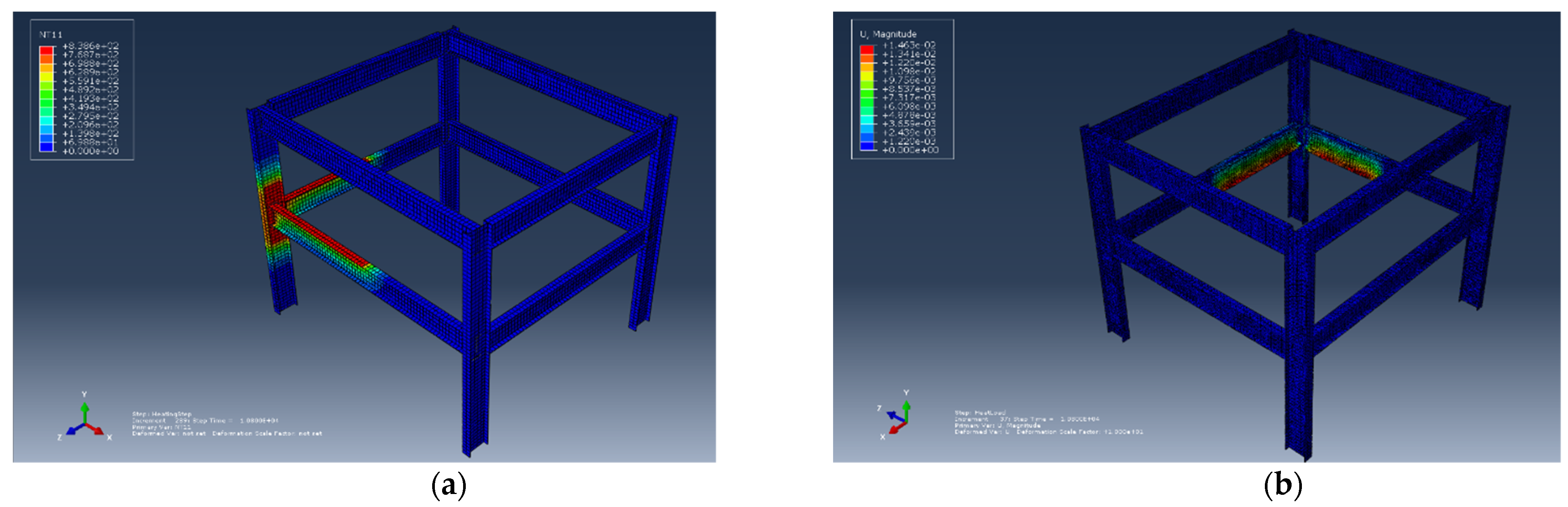
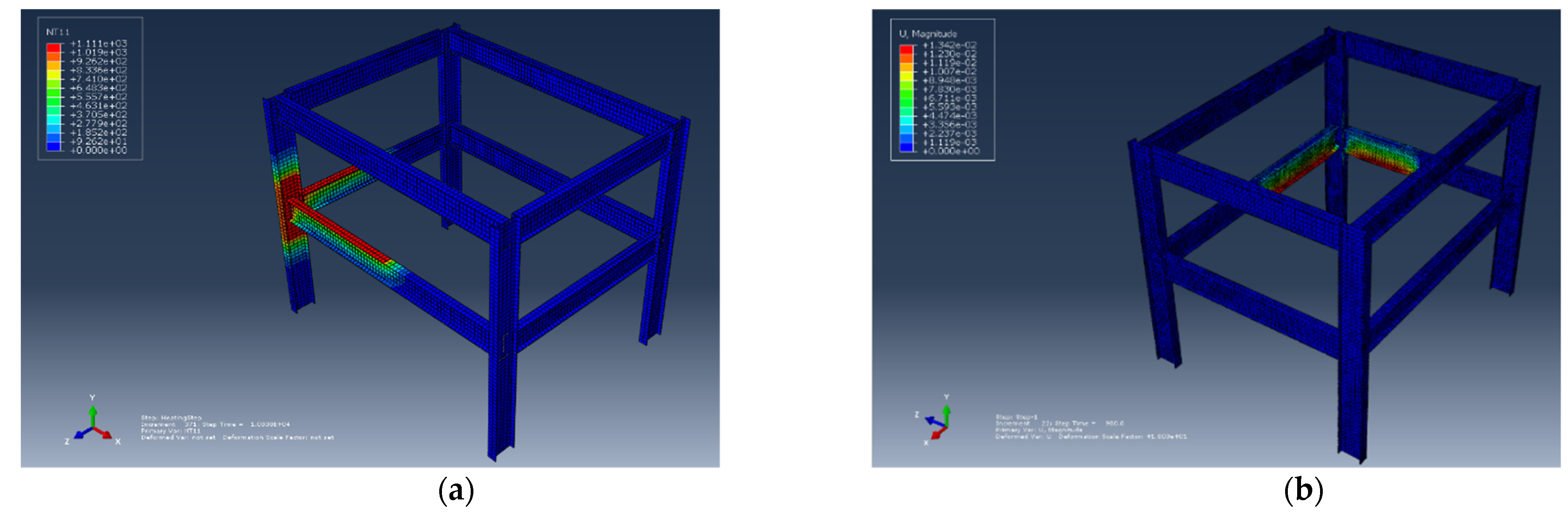
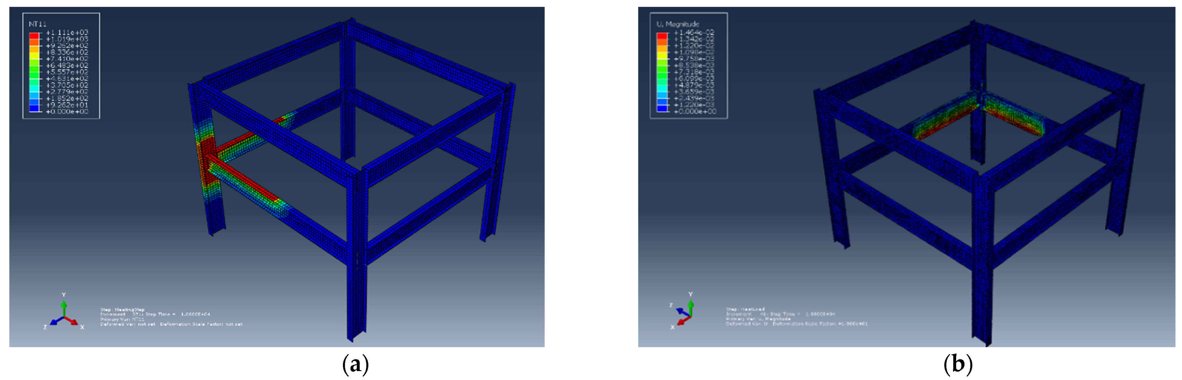
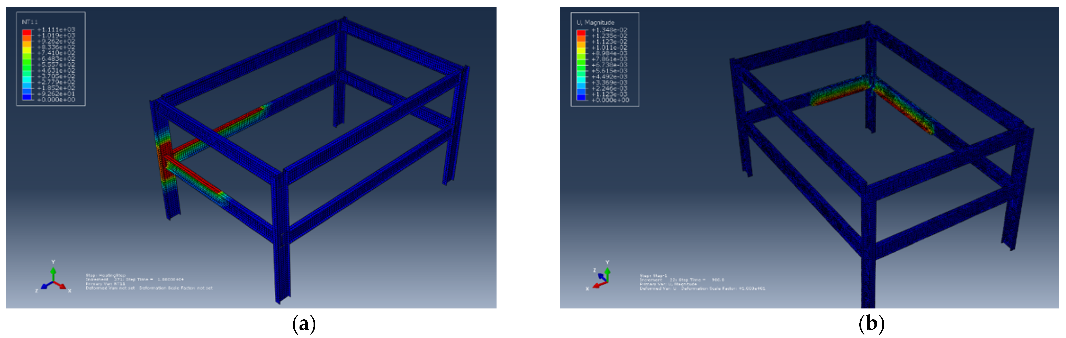
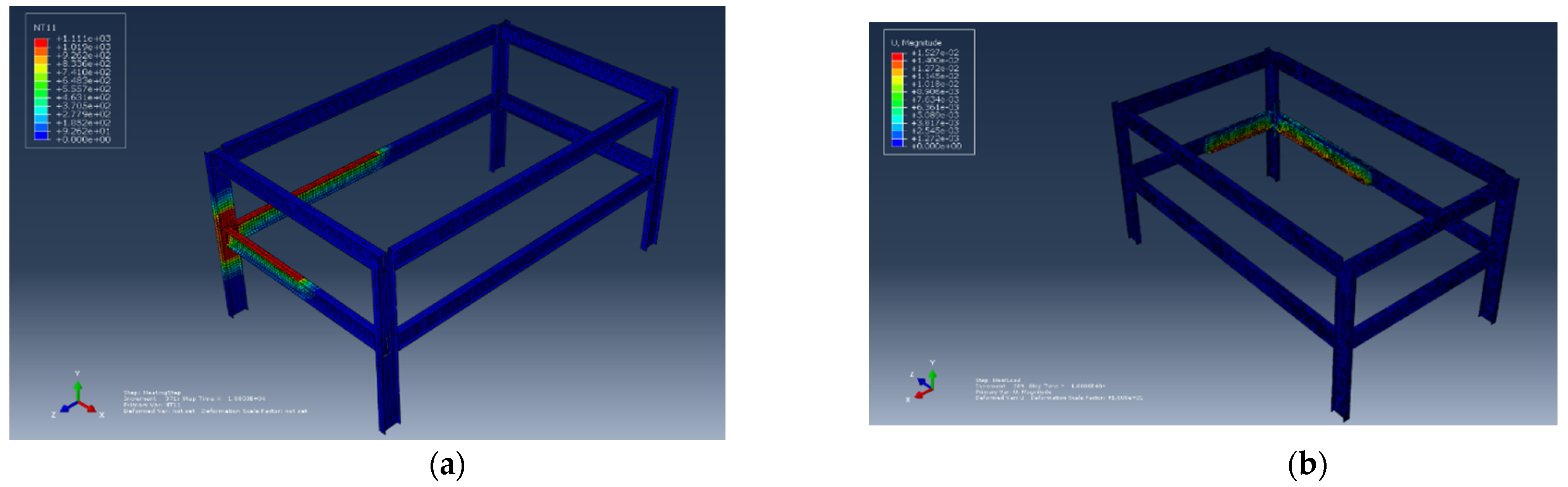
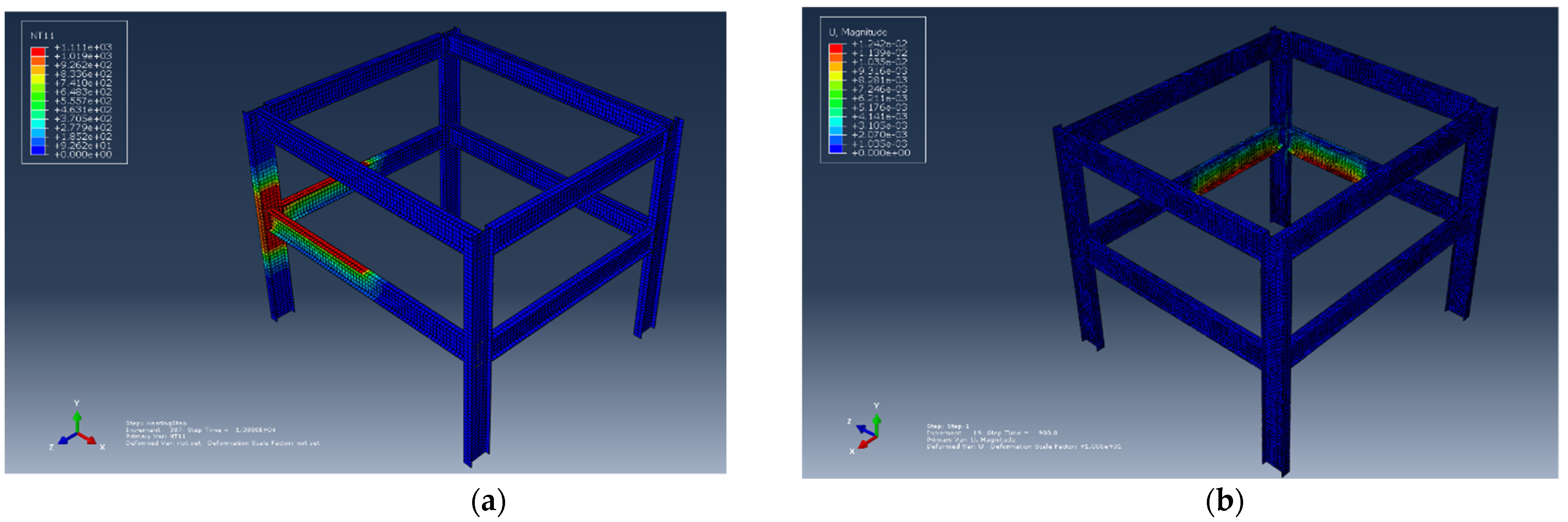
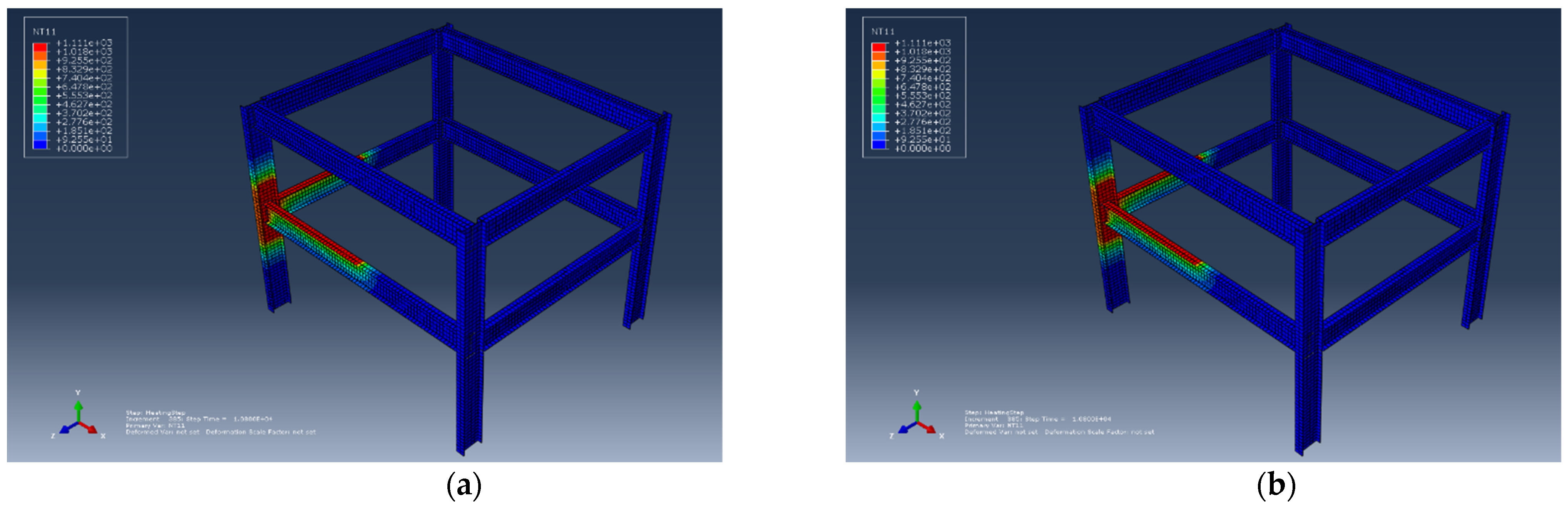
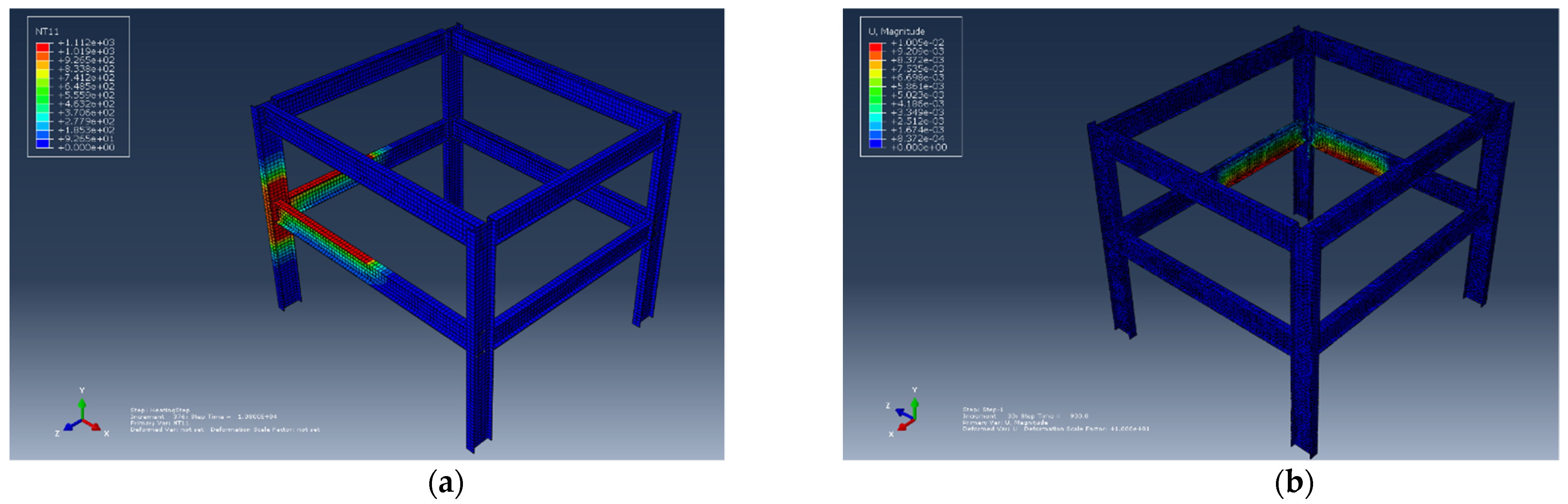
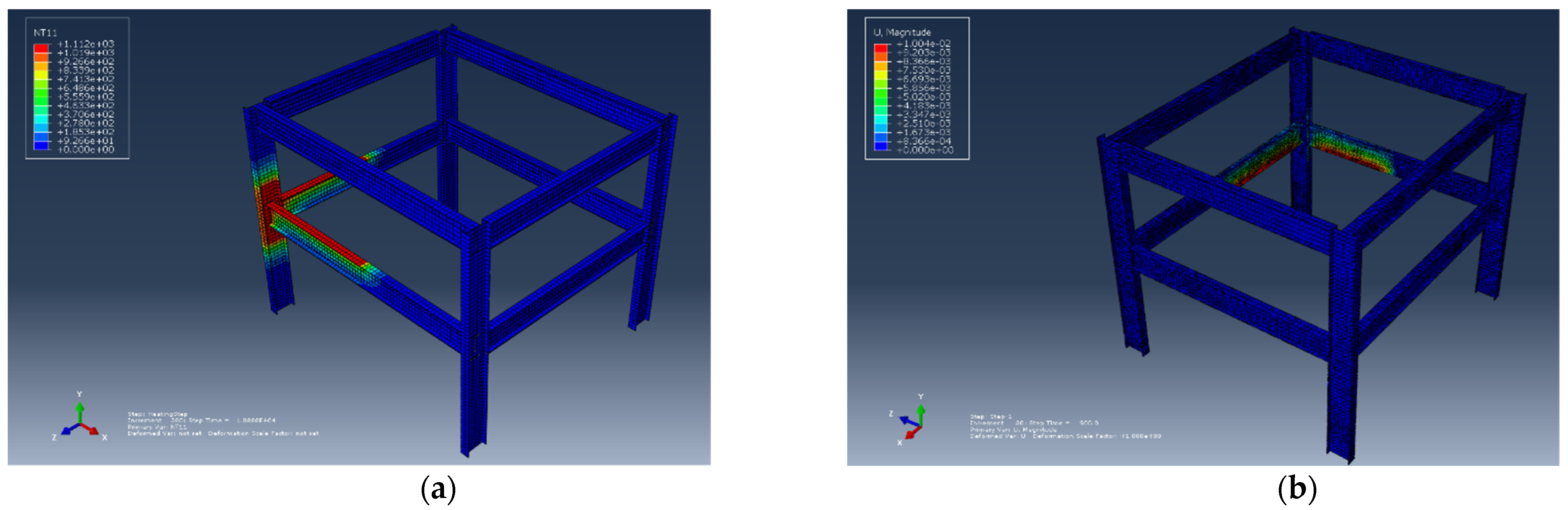
4.1. Effect of Opening Factor

The first set of results were obtained from both finite element analyses: (1) Heat transfer analysis, and (2) heat load analysis corresponded to the different opening factors obtained from the Monte Carlo simulation (Table 2). The different opening factors were applied to a steel frame with fixed dimensions (5.5 × 7 m) in terms of temperature amplitudes The results of the heat transfer load are shown in the form of nodal temperatures (NT11), whereas the results obtained from the mechanical analysis are shown in the form of displacement (U).
  • Scenario 1: An opening factor with a value of 0.0251 was used, and the corresponding results are shown in Figure 1a,b.
Figure 1. Effect of opening factors. (a) The nodal temperature corresponding to the opening factor of 0.0251. (b) The displacement corresponding to the opening factor of 0.0251.
Fire 05 00025 g001
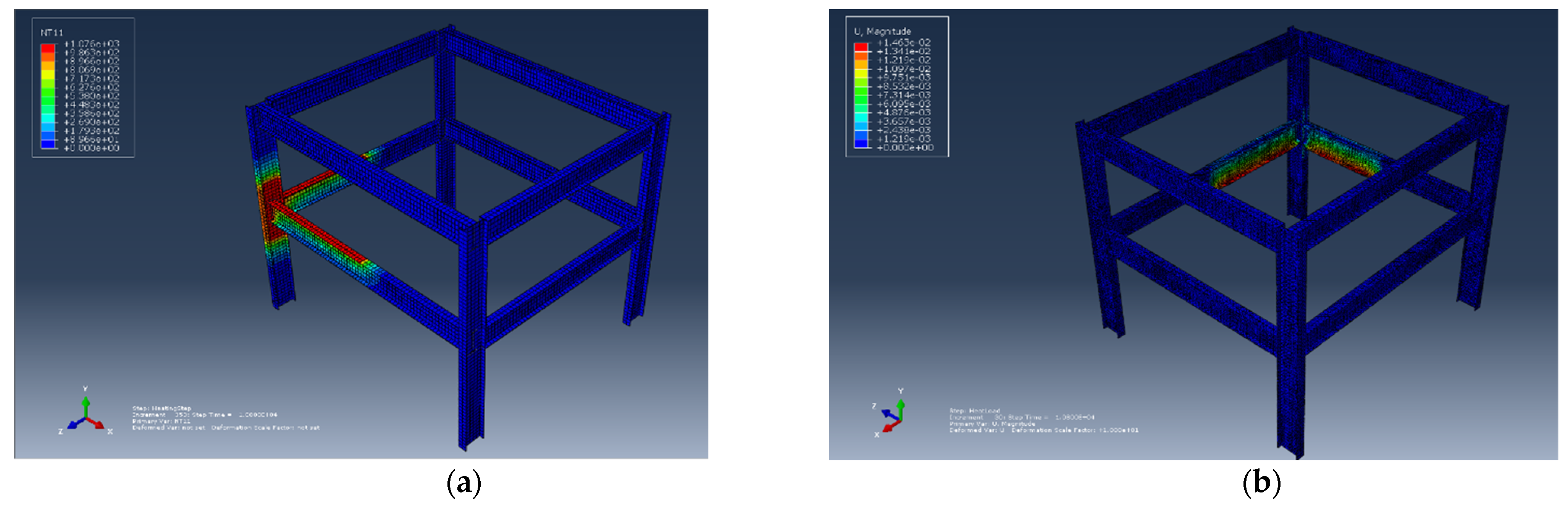
  • Scenario 2: An opening factor with a value of 0.0554 was used, and the corresponding results are shown in Figure 2a,b.
Figure 2. Effect of opening factors. (a) The nodal temperature corresponding to the opening factor of 0.0554. (b) The displacement corresponding to the opening factor of 0.0554.
Fire 05 00025 g002
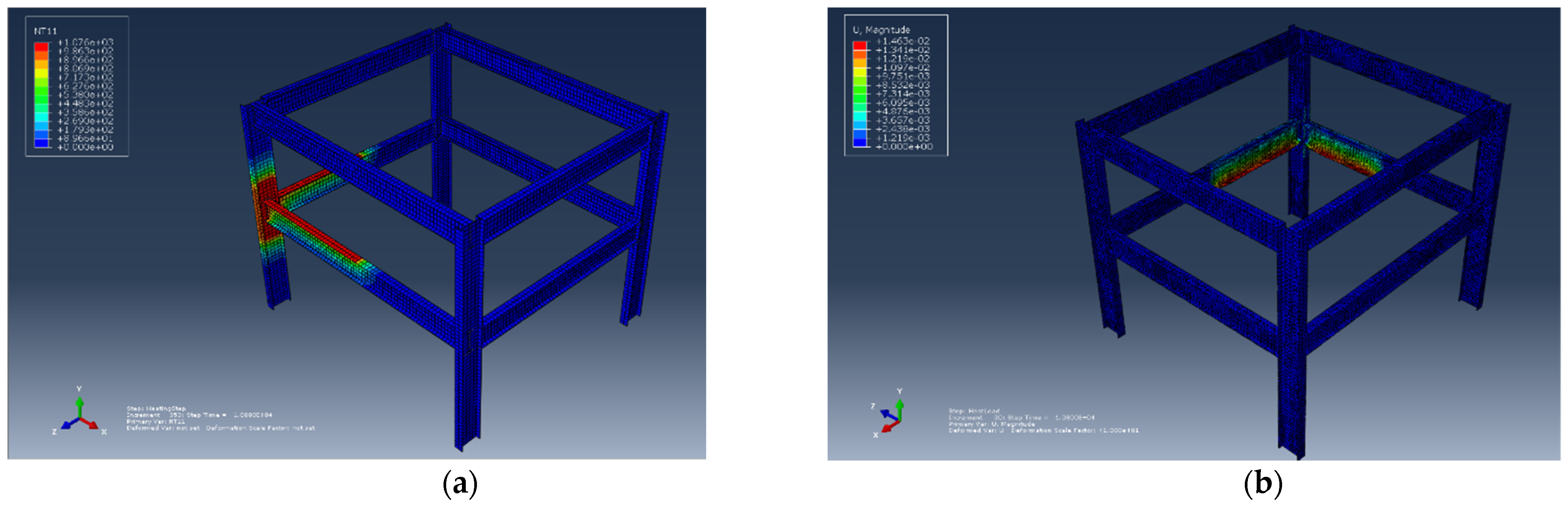
  • Scenario 3: An opening factor with a value of 0.1129 was used, and the corresponding results are shown in Figure 3a,b.
Figure 3. Effect of opening factors. (a) The nodal temperature corresponding to the opening factor of 0.1129. (b) The displacement corresponding to the opening factor of 0.1129.
Fire 05 00025 g003
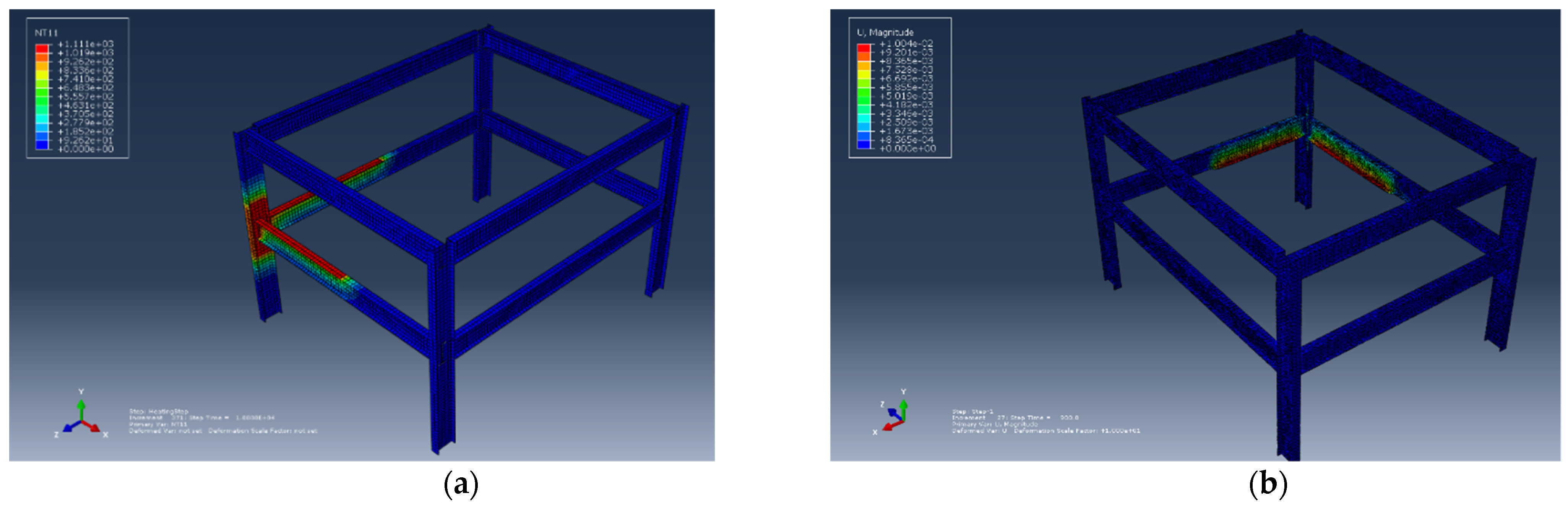
  • Scenario 4: An opening factor with a value of 0.1689 was used, and the corresponding results are shown in Figure 4a,b.
Figure 4. Effect of opening factors. (a) The nodal temperature corresponding to the opening factor of 0.1961. (b) The displacement corresponding to the opening factor of 0.1961.
Fire 05 00025 g004
  • Scenario 5: An opening factor with a value of 0.1961 was used, and the corresponding results are shown in Figure 5a,b.
Figure 5. Effect of opening factors. (a) The nodal temperature corresponding to the opening factor of 0.0554. (b) The displacement corresponding to the opening factor of 0.0554.
Fire 05 00025 g005

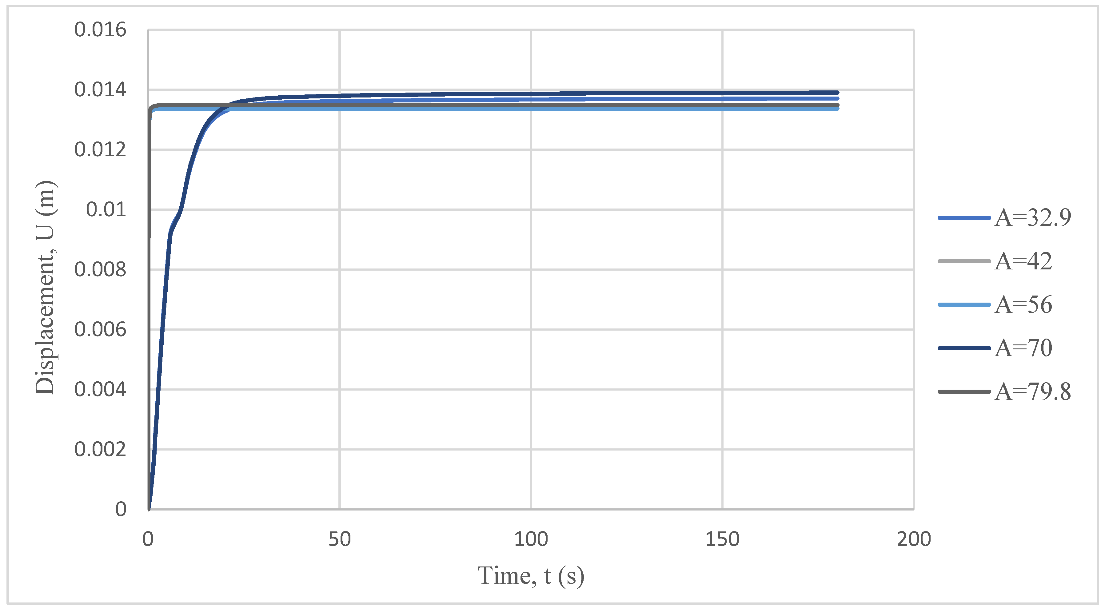
4.2. Effect of Compartment Area

The second set of results shown in this section represent the finite element analyses that correspond to the different compartment area dimensions (Table 2). While the dimension of the plan of the steel frame changed, the temperature amplitude and heat load remained constant. In order to achieve the desired compartment area size, one of the beams was given a fixed length of 7 m, while the other beam changes with every scenario. The results are represented below in the form of NT11 and U for each scenario generated by the Monte Carlo simulation.
  • Scenario 1: A compartment area with a size of 32.9 m2 was modelled, and the beam lengths were 7 and 4.7 m in length. The corresponding results are shown in Figure 6a,b.
Figure 6. Effect of Compartment Area. (a) The nodal temperature corresponding to the compartment area of 32.9 m2. (b) The displacement corresponding to compartment area of 32.9 m2.
Fire 05 00025 g006
  • Scenario 2: A compartment area with a size of 42 m2 was modelled, and the beams were 7 and 6 m long. The corresponding results are shown in Figure 7a,b.
Figure 7. Effect of Compartment Area. (a)The nodal temperature corresponding to the compartment area of 42 m2. (b) The displacement corresponding to the compartment area of 42 m2.
Fire 05 00025 g007
  • Scenario 3: A compartment area with a size of 56 m2 was modelled, and the beams were 7 and 8 m long. The corresponding results are shown in Figure 8a,b.
Figure 8. Effect of Compartment Area. (a) The nodal temperature corresponding to the compartment area of 56 m2. (b) The displacement corresponding to the compartment area of 56 m2.
Fire 05 00025 g008
  • Scenario 4: A compartment area with a size of 70 m2 was modelled, and the beams were 7 and 10 m long. The corresponding results are shown in Figure 9a,b.
Figure 9. Effect of Compartment Area. (a) The nodal temperature corresponding to compartment area of 70 m2. (b) The displacement corresponding to to compartment area of 70 m2.
Fire 05 00025 g009
  • Scenario 5: A compartment area with a size of 79.8 m2 was modelled, and the beams were 7 and 11.4 m long. The corresponding results are shown in Figure 10a,b.
Figure 10. Effect of Compartment Area. (a) The nodal temperature corresponding to the compartment area of 79.8 m2. (b) The displacement corresponding to the compartment area of 79.8 m2.
Fire 05 00025 g010

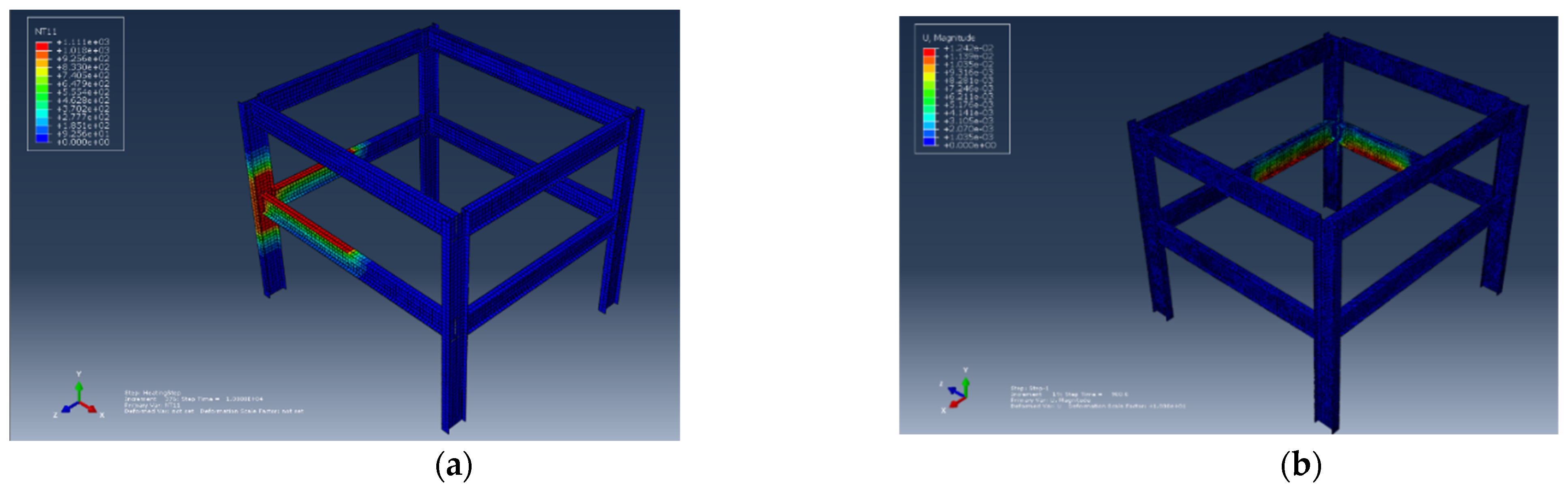
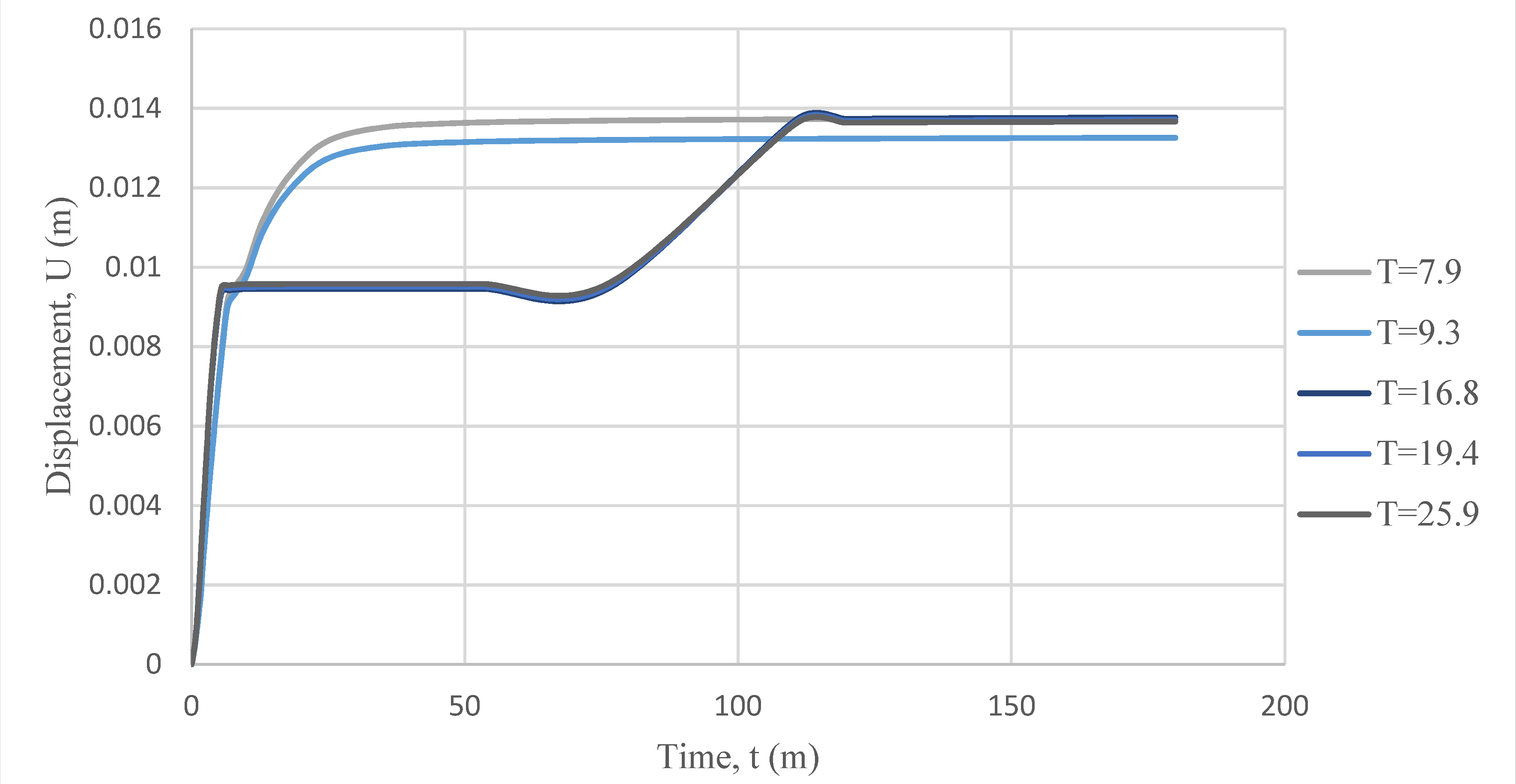
4.3. Effect of Flange Thickness

The third and last set of results represented in this section are related to the beam flange thickness. The thickness of the flange varied from 7.9 to 25.8 mm while the dimensions of the steel frame including the beams webs were fixed. The temperature amplitude and heat load applied to the structures were also fixed. The results represented are in the form of NT11 and U.
  • Scenario 1: The thickness of the flange was set to 7.9 mm, and the corresponding results are shown in Figure 11a,b.
Figure 11. Effect of flange thickness. (a) The nodal temperature corresponding to the flange thickness of 7.9 mm. (b) The displacement corresponding to the flange thickness of 7.9 mm.
Fire 05 00025 g011
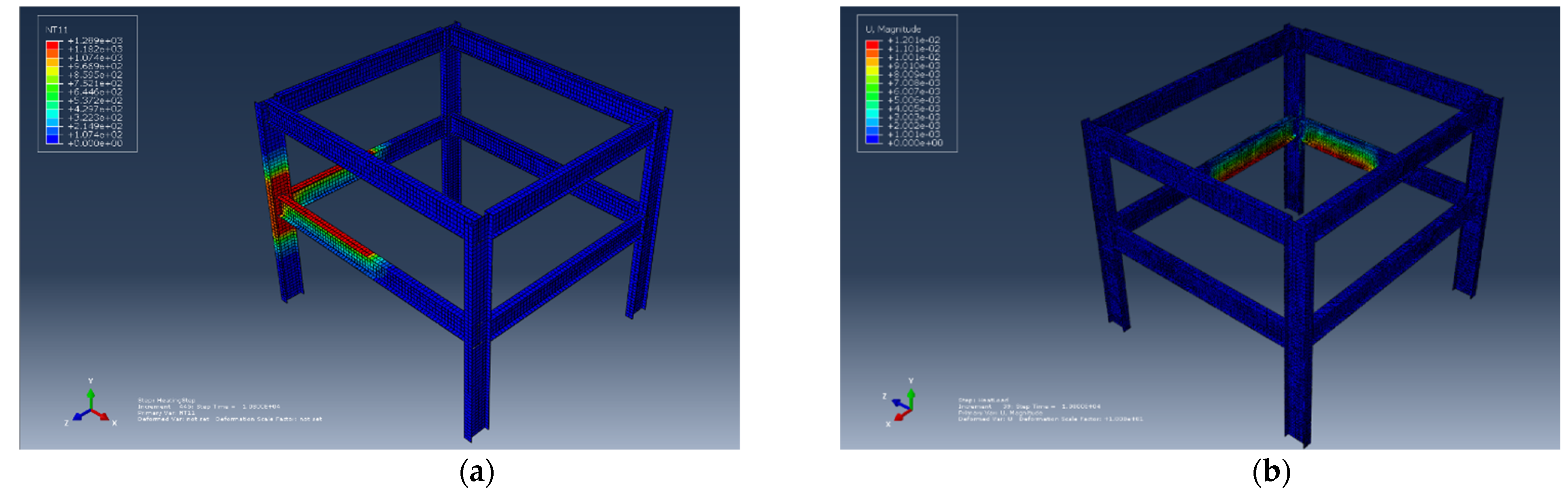
  • Scenario 2: The thickness of the flange was set to 9.3 mm, and the corresponding results are shown in Figure 12a,b.
Figure 12. Effect of flange thickness. (a) The nodal temperature corresponding to flange thickness of 9.3 mm. (b) The displacement corresponding to flange thickness of 9.3 mm.
Fire 05 00025 g012
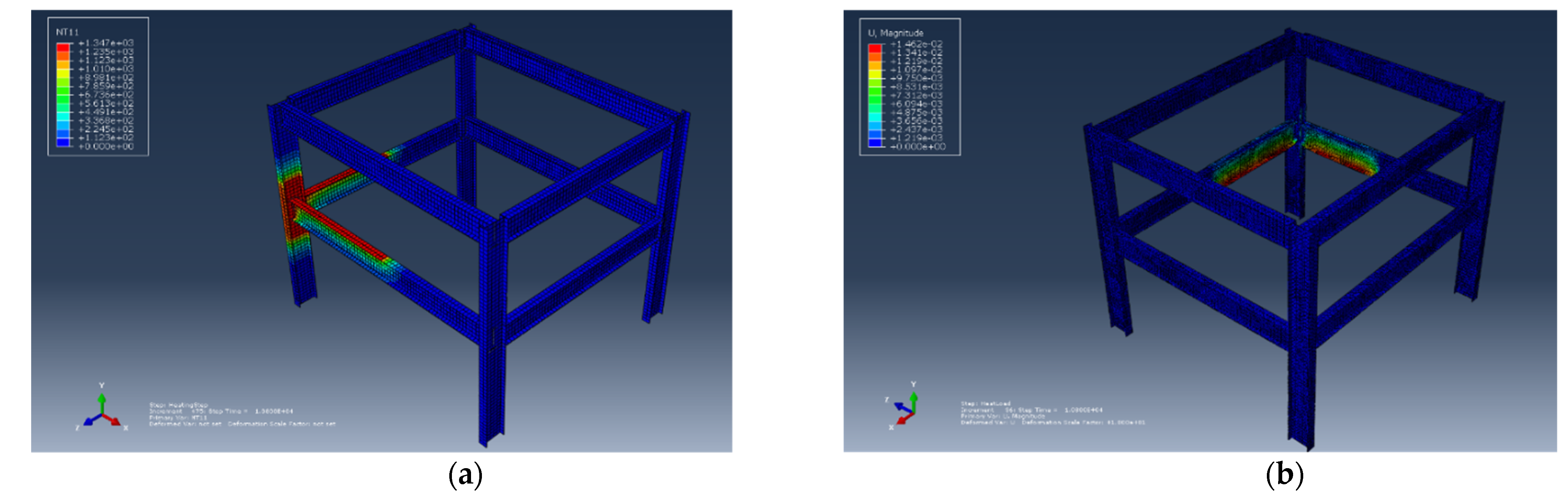
  • Scenario 3: The thickness of the flange was set to 16.7 mm, and the corresponding results are shown in Figure 13a,b.
Figure 13. Effect of flange thickness. (a) The nodal temperature corresponding to flange thickness of 16.7 mm. (b) The displacement corresponding to flange thickness of 16.7 mm.
Fire 05 00025 g013
  • Scenario 4: The beam flange thickness was set to 19.3 mm, and the corresponding results are shown in Figure 14a,b.
Figure 14. Effect of flange thickness. (a) The nodal temperature corresponding to flange thickness of 19.3 mm. (b) The displacement corresponding to flange thickness of 19.3 mm.
Fire 05 00025 g014
  • Scenario 5: The beam flange thickness was set to 25.8 mm, and the corresponding results are shown in Figure 15a,b.
Figure 15. Effect of flange thickness. (a) The nodal temperature corresponding to flange thickness of 25.8 mm. (b) The displacement corresponding to flange thickness of 25.8 mm.
Fire 05 00025 g015

4.4. Summary

From the parametric temperature-time curve Equation (1), it is clear to see that the opening factor plays an important role when it comes to determining the spread time of the fire along with the gas temperature increase in the fire compartment. Therefore, when looking at the gas temperature curves obtained from the different opening factors, it can be observed that the larger the opening factor is, the higher the gas temperature will be. The highest opening factor reaches the highest temperature in the shortest time. In fact, the highest gas temperature reached was by the largest opening factor, around 1300 °C. This is almost twice as much as the maximum gas temperature reached by the smallest opening factor, which was around 800 °C. However, the maximum specified limit of opening factor by Eurocode is 0.2.
From the ABAQUS model, it can be also seen that with different opening factors, the regions with the highest nodal temperatures were the upper flanges of both the beams and the inner web of the column, which was expected due to the fact that the load in both analyses was applied in those regions. The highest observed nodal temperature was found to be 1347 °C, corresponding to the opening factor of 0.1961; similar results were obtained for the opening factor of 0.1689, where it was around 1343 °C. On the other hand, the lowest observed temperature was found when the opening factor was 0.0251, where the temperature only reached 838.6 °C. When compared to the recorded temperatures from the Cardington tests [5], the temperatures from the numerical analysis are higher. In fact, the maximum nodal temperatures observed here are almost the same as the gas temperatures reached. This is mainly due to the fact that the steel was designed to be unprotected and there were no slabs modelled. Thus, the upper flange of the beam has a hotter temperature because it is in direct contact with the gas temperature.
The maximum displacement in the y-direction was plotted for the different opening factors as shown in Figure 16. In general, all beams started to deflect at around the same time; however, the highest deflection recorded was associated with the one of the highest opening factors (O = 0.1689), where it reached to around 0.014 m.
The results of the displacement in the y-direction for the different compartment areas are plotted in Figure 17. The plot shows that the highest deflection recorded was for the area of 70 m2, and it was around 0.014 m. It was also noted that in general there were around two general trends followed: one was followed by the plots corresponding to both 32.9 and 70 m2, and the other one followed by the remaining three. However, the latter curves started to deflect quicker than the former. The reason for this could be the fact that the results extracted from the model were chosen at random, even though an average of value was taken from three different nodes to minimize errors.
The displacement in the y-direction corresponding to the different flange thickness are plotted in Figure 18. From the figure, it can be said that the beams with the thinner flange thickness deflected quicker than the thicker flanges, which can be explained by the amount of time it takes for the heat to radiate from the top flange to the bottom one.
From all scenarios, it can be observed that the general behavior of the beam is similar, despite the different factors affecting the final result. This is not surprising because in some cases the heat load applied or the compartment area was fixed.. From the general displaced shapes for all cases, shown in Section 4, it is safe to say that the expansion co-efficient of steel had the most influence when it comes to heat load, even though it was also observed that some of the results are exaggerated in some cases, such as the nodal temperatures; this is mainly due to the absence of the slab.
As explained in [14], the tortional restraint is very important for the bare steel beams. It should be modeled in the ABAQUS model, but in reality, the beams are restrained directly by the slabs, which actually help to resist the lateral tortional buckling of the beam. We did not model the lateral restraint so as to provide a worst-case scenario for the study. The fire protection is an important factor affecting the global and local response of a structure on fire, but in this study, non-fire protection is assumed; this also provided a worst-case scenario for the study.
As explained in [15,16], the joints play an important role in the local and global behavior of the structure, as the moment and rotation capacity of the joints will affect the response of the structure. Therefore, the most accurate way to assess the joints is to physically model the bolts and endplate. Attempts have been made by the authors, but for a 3D frame system, the modeling of the bolted connection causes a convergence problem in the model, due to the complexity of the frame. Therefore, the beams are directly tied to the columns to replicate a perfect rigid connection, to reduce the computational cost while remaining reasonably accurate.
A further study will be performed by the authors to address the above limitations.

5. Conclusions

The aim of this project was to apply a parametric study of a steel frame in fire through sequential thermal and mechanical analyses. A two-story steel frame structure was simulated to investigate the influence of the opening factor, compartment area, and beam flange thickness using a Monte Carlo simulation to generate the random parameters. The following conclusions can be made:
  • The opening factor was found to be the parameter with the most influence on the rate of spread and temperature increase in the fire compartment.
  • The flange thickness also has significant influence on the response of structural members, due to its influence on the section factors.
  • The compartment area has less of an effect on the response of the structural member

Author Contributions

Conceptualization, F.F. Investigation, R.A. and F.F.; Methodology, F.F.; Supervision, F.F.; original draft, R.A.; Writing—review & editing, F.F. All authors have read and agreed to the published version of the manuscript.

Funding

This research received no external funding.

Data Availability Statement

Not applicable.

Conflicts of Interest

The authors declare no conflict of interest.

Nomenclature

AcomArea of Compartment
AtArea of total internal surface of fire compartment
AvArea of ventilation
BWidth of Section
bThermal Diffusivity
CSpecific Heat
CaSpecific Heat of Steel
DDepth of Section
heqHeight of Openings
OOpening Factor
TThickness of Flange
tTime
UDisplacement
αExpansion Co-efficient
εpPlastic Strain
θaSteel’s Temperature
θgGas Temperature in the Fire Compartment
λThermal Conductivity
λaThermal Conductivity of Steel
ρDensity
ρaDensity of Steel
σStephan-Boltzmann Constant
σyYield Stress
νPoisson’s Ratio

References

  1. Fitzgerald, R.W. Structural Integrity During Fire; National Fire Protection Association: Quincy, MA, USA, 1997. [Google Scholar]
  2. Bailey, C. Prescriptive Design Methods in Fire. 2004. Available online: http://www.mace.manchester.ac.uk/project/research/structures/strucfire/Design/prescriptive/default.htm (accessed on 5 January 2018).
  3. Bailey, C. Zone Models. 2004. Available online: http://www.mace.manchester.ac.uk/project/research/structures/strucfire/Design/performance/fireModelling/zoneModels/default.htm?p=28|#28 (accessed on 5 January 2018).
  4. Fu, F. Advanced Modelling Techniques in Structural Design; John Wiley & Sons, Ltd.: Chichester, UK, 2015. [Google Scholar]
  5. Fu, F. Structural Analysis and Design to Prevent Disproportionate Collapse; CRC Press: Boca Raton, FL, USA, 2016. [Google Scholar]
  6. Fu, F. Fire Safety Design for Tall Buildings; Taylor Francis: Boca Raton, FL, USA, 2021; ISBN 978-0-367-44452-5. [Google Scholar]
  7. Fu, F. Design and Analysis of Tall and Complex Structures; Butterworth-Heinemann: Oxford, UK, 2018; ISBN 978-0-08-101121-8. [Google Scholar]
  8. Tavelli, S.; Rota, R.; Derudi, M. A critical comparison between CFD and zone models for the consequence analysis of fires in congested environments. AIDIC 2014, 36. [Google Scholar] [CrossRef]
  9. Tagawa, H.; Miyamura, T.; Yamashita, T.; Kohiyama, M.; Ohsaki, M. Detailed finite element analysis of full-scale four-storey steel frame structure subjected to consecutive ground motions. Jpn. Int. J. High-Rise Build. 2015, 4, 65–73. [Google Scholar]
  10. Wong, J. Reliability of Structural Fire Design; University of Canterbury: Christchurch, New Zealand, 1999. [Google Scholar]
  11. MathWorks Perform Sensitivity Analysis through Random Parameter. 2018. Variation. Available online: https://www.mathworks.com/discovery/monte-carlo-simulation.html (accessed on 28 March 2018).
  12. EN 1991-1-2 (2005b)Eurocode 1. Actions on Structures, Part 1-2: General Actions—Actions on Structures Exposed to Fire, Commission of the European Communities: Brussels, Belgium, 2005.
  13. EN 1993-1-2 (2005a)Eurocode 3. Design of Steel Structures, Part 1-2; General Rules. Structural Fire Design, Commission of the European Communities: Brussels, Belgium, 2005.
  14. Tartaglia, R.; D’Aniello, M.; Wald, F. Behaviour of seismically damaged extended stiffened end-plate joints at elevated temperature. Eng. Struct. 2021, 247, 113193. [Google Scholar] [CrossRef]
  15. Qiang, X.; Bijlaard, F.S.K.; Kolstein, H.; Jiang, X. Behaviour of beam-to-column high strength steel endplate connections under fire conditions—Part 2: Numerical study. Eng. Struct. 2014, 64, 39–51. [Google Scholar] [CrossRef]
  16. Shakil, S.; Lu, W.; Puttonen, J. Response of high-strength steel beam and single-storey frame in fire: Numerical simulation. J. Constr. Steel Res. 2018, 148, 551–561. [Google Scholar] [CrossRef]
Figure 16. Beam displacement in the y-direction corresponding to the different opening factors.
Fire 05 00025 g016
Figure 17. Beam displacement in the y-direction corresponding to the different compartment areas.
Fire 05 00025 g017
Figure 18. Beam displacement in the y-direction corresponding to the different beam flange thickness.
Fire 05 00025 g018
Table 1. Range of the parameters used for Monte Carlo simulation.
Opening Factor, O (m1/2)0.02 ≤ O ≤ 0.2
[12]
Compartment Area, Acom (m2)Acom ≤ 500
[12]
Beam Flange Thickness, T (mm)7.5 < T < 55
[13]
Table 2. Chosen values from the Monte Carlo simulation.
Opening Factor, O (m1/2)O = 0.0251
O = 0.0554
O = 0.1129
O = 0.1689
O = 0.1961
Compartment Area, Acom (m2)Acom = 32.9
Acom = 42
Acom = 56
Acom = 70
Acom = 79.8
Beam Flange Thickness, T (mm)T = 7.9066
T = 9.3202
T = 16.7989
T = 19.3693
T = 25.8854
Publisher’s Note: MDPI stays neutral with regard to jurisdictional claims in published maps and institutional affiliations.

