Escape Route Index: A Spatially-Explicit Measure of Wildland Firefighter Egress Capacity

Abstract

For wildland firefighters, the ability to efficiently evacuate the fireline is limited by terrain, vegetation, and fire conditions. The impacts of terrain and vegetation on evacuation time to a safety zone may not be apparent when considering potential control locations either at the time of a wildfire or during pre-suppression planning. To address the need for a spatially-explicit measure of egress capacity, this paper introduces the Escape Route Index (ERI). Ranging from 0 to 1, ERI is a normalized ratio of the distance traveled within a time frame, accounting for impedance by slope and vegetation, to the optimal distance traveled in the absence of these impediments. An ERI approaching 1 indicates that terrain and vegetation conditions should have little impact on firefighter mobility while an ERI approaching 0 is representative of limited cross-country travel mobility. The directional nature of evacuation allows for the computation of four ERI metrics: (1) ERI_mean (average ERI in all travel directions); (2) ERI_min (ERI in direction of lowest egress); (3) ERI_max (ERI in direction of highest egress); and (4) ERI_azimuth (azimuth of ERI_max direction). We demonstrate the implementation of ERI for three different evacuation time frames (10, 20, and 30 min) on the Angeles National Forest in California, USA. A previously published, crowd-sourced relationship between slope and travel rate was used to account for terrain, while vegetation was accounted for by using land cover to adjust travel rates based on factors from the Wildland Fire Decision Support System (WFDSS). Land cover was found to have a stronger impact on ERI values than slope. We also modeled ERI values for several recent wildland firefighter entrapments to assess the degree to which landscape conditions may have contributed to these events, finding that ERI values were generally low from the crews’ evacuation starting points. We conclude that mapping ERI prior to engaging a fire could help inform overall firefighter risk for a given location and aid in identifying locations with greater egress capacity in which to focus wildland fire suppression, thus potentially reducing risk of entrapment. Continued improvements in accuracy of vegetation density mapping and increased availability of light detection and ranging (lidar) will greatly benefit future implementations of ERI.

1. Introduction

Escape routes are some of the most important safety measures available to wildland firefighters, acting as pre-defined pathways for firefighters to access a safety zone or other low-risk area from their current position [1]. They are an integral component of the Lookouts, Communications, Escape routes, and Safety zones (LCES) safety protocol and are imbedded throughout the 10 Standard Firefighting Orders and the 18 Situations that Shout Watch Out [2,3]. The Incident Response Pocket Guide, which is used by all US wildland firefighters, describes some ideal characteristics of escape routes, including having more than one, avoiding steep uphill routes, and timing them considering the slowest crewmember given current levels of fatigue [4]. In order to be maximally-effective, escape routes should provide fire crews with a positive Margin of Safety (MOS) [5]. MOS is defined as the difference between the time it takes a fire to reach a given location, such as a safety zone (T1) and the time it takes a fire crew to reach that same location (T2) (Figure 1). If T1 is greater than T2 (positive MOS), the crew should reach the safety zone without harm; however, if T2 is greater than T1 (negative MOS), the crew is at risk of becoming entrapped and suffering a burnover.

Both T1 and T2 are difficult to predict accurately in the field. T1 is controlled by fire behavior, the drivers of which are fuel, weather, and topography [6]. Due to both the complexity of modeling fire behavior and the importance of being able to understand how fire moves through and affects a landscape, there is an extensive body of literature and several operational products aimed at predicting fire behavior (for a review of fire behavior modeling systems, please refer to [7]). Considerably less attention has been devoted to predicting T2, which is controlled by a combination of internal factors (e.g., height, weight, fitness and endurance levels, and load carriage) and external factors (e.g., landscape and environmental conditions). Internal factors are highly variable within a population, but if a fire crew moves as a unit, then they are only as fast as the slowest individual in the group. This makes modeling population-level differences as a function of external factors more important than modeling individual differences. An additional benefit to focusing on external factors is that most external factors can be mapped on a broad spatial scale using a combination of remote sensing and geographic information systems (GIS).

The most important external factors that affect one’s ability to efficiently move through a given landscape include terrain slope, ground surface condition (e.g., roughness, firmness, and stability), and the presence, abundance, and arrangement of vegetation [8]. The effects of slope on travel rates have been studied since the nineteenth century, and several models for predicting travel rates based on slope have been developed, including the widely-used Naismith’s Rule and Tobler’s Hiking Function [9,10]. Though widely-cited, these travel rate functions lack the scientific rigor inherent to large sample sizes, GPS-driven instantaneous travel rates, and modern statistical modeling techniques. A recent study by Campbell et al. [11] overcame previous limitations, producing an improved slope-travel rate predictive model based on a very large database of GPS tracks harvested from the widely-used mobile fitness tracking application Strava, and light detection and ranging (lidar)-derived terrain slope data. At present, their resulting model represents the most accurate understanding of the relationship between slope and travel rates, and as such, will be used as the basis of simulating slope impedance in this study. Given the fact that digital elevation models (DEM) are available on a nationwide basis in the US as a part of the United States Geological Survey (USGS) 3D Elevation Program (3DEP) [12], a slope-based, spatially-explicit model for predicting optimal, or “least-cost” escape routes could be realized (e.g., [8,13]). However, to more accurately simulate movement in a wildland environment, the effects of land cover on travel rates also need to be taken into account.

The effects of ground surface condition and vegetation are both less well-understood and more difficult to map. In a review of the energetic costs associated with traversing a diversity of landscape conditions, Richmond et al. [14] identify four parameters that affect the efficiency of pedestrian movement in a wildland environment: (1) sinkage (how deep a foot will sink into the ground surface); (2) slipperiness (the relative friction of the ground surface); (3) roughness (the microtopography that controls foot placement on the ground surface); and (4) vegetation (the presence, abundance, and arrangement of physical impediments on top of the ground surface). The first three parameters can be categorized broadly as ground surface conditions, controlled primarily by a combination of soil type (e.g., clay vs. sand), soil condition (e.g., dry vs. wet), underlying geology (e.g., sedimentary vs. igneous), history of geomorphological activity (e.g., erosion vs. deposition), history of human activity (e.g., paved vs. natural) and presence and depth of snow or ice on the ground surface. The fourth parameter—vegetation—impedes movement in a variety of ways, including obstacle avoidance (avoiding dense patches of vegetation altogether, thus increasing travel distance and decreasing net travel rate), obstacle navigation (stepping over debris, crouching under branches, squeezing through gaps), friction (woody and/or foliar biomass resisting forward movement), and bushwhacking (physical alteration of the desired path requiring additional time and energy). Much of the research aimed at understanding how these different landscape conditions affect pedestrian movement stems from the field of applied physiology, where human experimentation dating back to the 1970s has yielded estimates for the energetic costs associated with traversing diverse landscape conditions. However, due to the complex and interacting nature of the effects of these four parameters, rather than quantifying the effects individually, they are typically described in terms of broadly-defined “terrain coefficients”, which represent the relative energetic costs associated with traversing a variety of general land cover types, as seen in

Table 1. Relative energetic cost of pedestrian movement through various land cover types, adapted from [15,16].

Land Cover	Relative Energy Cost
Blacktop surface	1.0
Dirt road	1.1
Light brush	1.2
Hard-packed snow	1.3
Heavy brush	1.5
Swampy bog	1.8
Loose sand	2.1
Soft snow (15 cm)	2.5
Soft snow (25 cm)	3.3
Soft snow (35 cm)	4.1

[15,16].

Campbell et al. [8] used airborne lidar remote sensing to derive continuous measures of slope, vegetation density, and ground surface roughness as the basis of travel impedance analysis. Absent direct quantification of ground surface condition and vegetation, land cover or fuel type can serve as a proxy, assuming that land cover classes or fuel types represent typical or average vegetation and ground surface conditions within each class. Alexander et al. [17] tested the combined effects of load carriage, terrain slope, and fuel type on wildland firefighter travel rates. They did not present specific multiplicative factors, such as those in Table 1 and travel rates were measured, rather than metabolic costs. The results show that open fuel types, such as grasslands and logging slash tend to promote the fastest travel, whereas lodgepole pine stands with an open understory increase travel time by a factor of about 1.3, and dense spruce and fir forests increased travel time by a factor of about 1.8. The Wildland Fire Decision Support System (WFDSS) uses land cover factors to adjust travel rates for its Ground Medevac Time dataset (

Table 2. Wildland Fire Decision Support System (WFDSS) travel rates based on slope and land cover, in miles per hour.

	Land Cover
Slope	Grass/Non-Burnable	Brush	Timber	Water
Flat (≤10°)	3.00	1.50	0.75	0.01
Moderate (10°–30°)	1.50	0.75	0.25	---
Steep (≥30°)	1.00	0.50	0.10	---

). This is a US nationwide GIS dataset representing transport time to the nearest hospital [18].

By combining the slope-travel rate function defined by Campbell et al. [11], and the land cover-travel rate effects defined by WFDSS [18], spatially-explicit escape route mapping could become a reality. However, as the National Wildfire Coordinating Group (NWCG) points out, escape routes are “probably the most elusive component of LCES” [19], as their effectiveness changes continuously throughout a day. Thus, to be useful for wildland firefighters, escape route mapping has to be done in real-time or near-real-time, which requires three things: (1) the location of the crew; (2) the location of the designated safety zone; and (3) the extent and predicted spread of the fire. In the absence of a widely-adopted, GPS-driven, mobile platform to implement such a real-time mapping effort, operational escape route mapping may not be currently feasible. However, even without knowing (1), (2), or (3) described above, one can still use pre-mapped terrain and land cover information to help wildland firefighters determine what areas have generally better or worse egress capacity.

The goal of this paper is to introduce the Escape Route Index (ERI), which is a spatially-explicit measure of relative egress capacity based on the effects of terrain slope and land cover on pedestrian travel rates. ERI is a suite of four spatial metrics aimed at capturing the directionally-specific effects of the landscape on travel rates: (1) ERI_mean (average ERI in all travel directions from a given starting location); (2) ERI_min (ERI in the direction of lowest/worst egress); (3) ERI_max (ERI in the direction of highest/best egress); and (4) ERI_azimuth (azimuth of the direction of highest/best egress). When mapped in advance of a wildland fire, the ERI can help wildland firefighters identify potential control locations in areas with favorable conditions for evacuation. We first describe the conceptual basis of ERI, followed by a detailed description of how it is implemented in a geospatial environment. To demonstrate utility on a broad spatial scale, ERI is mapped throughout the entire Angeles National Forest (ANF) in southern California. Lastly, ERI is used to look back in time at previous wildland firefighter entrapment events to assess how slope and land cover may have contributed to the events.

2. Materials and Methods

2.1. Definition

ERI is a relative measure of egress capacity based on existing terrain and land cover conditions. It is measured as a ratio between the actual distance one can travel within a given time frame, and the optimal distance one can travel within that same time frame. Optimal distance is defined as the distance traveled from a given starting point in the absence of any landscape impediments. Actual distance is defined as the distance one can travel from a given starting point, as modeled in a geospatial environment, factoring in the decrease in travel rate caused by slope and land cover. Accordingly, ERI ranges from 0 to 1, where 0 indicates extremely poor egress, such that landscape conditions prevent any kind of movement from a given location, and 1 represents ideal egress. An ERI value of 0.5 would indicate that, under a given set of landscape impediments, one can travel 50% of the distance that could be covered in the absence of those impediments. Alternatively, it can be conceptualized in terms of a travel rate, such that an ERI of 0.5 means one could only evacuate a given location at 50% of the travel rate under optimal conditions.

To calculate ERI, you first need to establish the relative travel cost (a.k.a. impedance, resistance, friction), or inversely, the conductance associated with the landscape conditions of interest. A high travel cost (low travel conductance) means that one would move more slowly, whereas a low travel cost (high travel conductance) means that one would move more quickly. The choice of whether to use cost or conductance when simulating movement depends on the geospatial software being used. In this study, ERI is modeled entirely in R [20] using the gdistance library [21], which relies on conductance values, so the methods will be discussed under the conductance framework henceforth. Travel conductance can be an absolute measure, such as the rate of travel (in m s⁻¹) through a given environment. For example, on flat ground one may travel at 1 m s⁻¹, whereas on a steep slope one may travel at 0.5 m s⁻¹. Travel conductance can also be a relative measure, such as a multiplicative factor that modifies an absolute measure of conductance. For example, one may travel at 0.5x the travel rate through dense vegetation as compared to sparse vegetation. In this study, the absolute travel conductance values associated with terrain slope are derived from Campbell et al.’s [11] slope-travel rate function recommended for simulating an average hiking pace (Lorentz 5^th percentile), as follows:

$$v=c\left(\frac{1}{\pi b\left[1+{\left(\frac{\theta -a}{b}\right)}^2\right]}\right)+d+e\theta ,$$

(1)

where v is the absolute conductance measured as velocity in m s⁻¹, θ is slope in degrees, and a, b, c, d, and e are constants with the values −1.53, 14.04, 36.81, 0.32, and −0.0027, respectively. The relative travel conductance values associated with land cover are derived from WFDSS, with values taken from Table 2 converted into relative, per-slope-class multiplicative factors, rather than absolute travel rates. Those factors can be seen in

Table 3. Adaptation of the WFDSS estimated travel rates, where absolute travel rates are converted to per-slope-class travel rate conductance relative to traversing grass/non-burnable land cover.

	Land Cover
Slope	Grass/Non-Burnable	Brush	Timber	Water
Flat (≤10°)	1.000	0.500	0.250	0.003
Moderate (10°–30°)	1.000	0.500	0.167	---
Steep (≥30°)	1.000	0.500	0.100	---

.

When combined, the slope and land cover conductance values can be seen in Figure 2. For the purpose of this study, to avoid extrapolation of the Campbell et al. [11] travel rate function and to avoid modeling travel up or down very steep slopes, travel was restricted to directionally-specific slopes within ±30°. The operative term here is “directionally-specific”, because although it is extremely inefficient to travel directly up and down slopes of greater than 30°, such slopes are not entirely impassable, as one can travel up or down said slopes at an angle, such as in a switchback fashion. However, above a certain slope threshold, travel is entirely impassable (e.g., you can’t switchback up a cliff). For the purpose of this study, that completely impassable threshold was set to ±45°.

2.2. Calculation

To implement the ERI model spatially, we selected ANF in southern California as a test study area (Figure 3). ANF was chosen for three reasons: (1) to demonstrate model implementation on a practical spatial scale; (2) it features a high diversity of both terrain and land cover conditions; and (3) it is a very fire-prone area, with a history of wildland firefighter entrapments [22]. The model requires three spatial datasets as inputs: (1) a DEM; (2) a Landscape Fire and Resource Management Planning Tools (LANDFIRE) Existing Vegetation Type (EVT) dataset, both in raster format and at 30 m spatial resolution for consistency; and (3) a roads and trails dataset, in vector format. The DEM and LANDFIRE data were acquired within the extent of ANF, re-projected into the same coordinate system (NAD 1983 UTM Zone 11N), and co-registered spatially so that cells aligned perfectly within the same grid. At the time of writing, 2014 was the most recent year that LANDFIRE data were available for ANF. LANDFIRE data were reclassified into the WFDSS land cover classes based primarily on the National Vegetation Classification Standard (NVCS) order attribute, as shown in

Table 4. Lookup table for converting LANDFIRE EVT National Vegetation Classification Standard (NVCS) orders to WFDSS land cover types.

EVT NVCS Order	WFDSS Land Cover
Herbaceous/Nonvascular-Dominated	Grass/Non-Burnable
No Dominant Lifeform	Grass/Non-Burnable
Non-Vegetated (not EVT “Open Water”)	Grass/Non-Burnable
Non-Vegetated (EVT “Open Water”)	Water
Shrub-Dominated	Brush
Tree-Dominated	Timber

.

Because LANDFIRE data are generated at a spatial resolution of 30 m, only roads that are roughly at least 30 m wide are captured in the dataset. Thus, many smaller roads and trails are not represented. However, given their relative low slope, ground surface stability, and lack of vegetation impedance, roads and trails tend to promote maximally efficient travel, where available [8,10,16,17]. Accordingly, roads and trails data were acquired from two sources: (1) FSTopo, which is the USDA Forest Service’s primary base map series and contains detailed roads and trails data throughout Forest Service lands in the US; and (2) The USGS National Map, which contains roads and trails data throughout the entire US. These roads and trails were converted to raster format with the same resolution as, and co-registered to, the elevation and land cover data. Roads and trails were merged with the land cover, and classified as “Grass/Non-Burnable”, representing the class of highest travel conductance.

Calculation of ERI requires that a time frame be chosen to facilitate actual vs. optimal travel distance calculation from a given starting point. For the purpose of this study, to compare the effects of different time frames on the resulting ERI values, three times were chosen: 10 min, 20 min, and 30 min. These times were chosen to reflect reasonable travel times from the fireline to a safety zone, according to historical, well-documented wildland firefighter entrapments [23], while balancing the computational cost associated with processing longer travel times. Thus, the ERI₁₀ indicates, for example, how far or fast one can travel in 10 min from a starting point with existing landscape impediments relative to how far or fast one could travel within that same time frame in the absence of any impediments.

ERI modeling was performed on a cell-by-cell basis throughout ANF as follows (Figure 4). It is worth noting that while Figure 4 depicts the process for modeling ERI for a single starting location (Figure 4a) within ANF at a single time frame (30 min), this same procedure was performed on every raster cell within the study area for each of the three time frames. The two input variables, a DEM and the reclassified LANDFIRE EVT dataset with the roads and trails modification, can be seen in Figure 4b. From the starting point, total travel time on a cell-by-cell basis was calculated using Dijkstra’s algorithm [24], as implemented in the accCost function within the gdistance library [21] in R (Figure 4c). A travel time threshold was then applied to the accumulative cost raster for the time frame of interest (in the example figure, 30 min) and converted to a vector polygon (Figure 4d). This polygon represents the actual travel distance one can traverse from the starting point. However, as can clearly be seen, not all travel directions provide the same egress capacity. Thus, to calculate directionally-specific travel distances, 100 evenly-spaced points were generated along the polygon boundary and distances were calculated from the starting point to those edge points (Figure 4d). Optimal travel conductance conditions were calculated based on the fastest combination of slope and land cover conditions seen in Figure 2. The land cover of highest conductance was grass/non-burnable, and the slope of highest conductance was -1.85°, which was determined by performing an optimization of Equation (1). Accordingly, for each of the three time frames, an optimal travel distance was calculated, the results of which can be seen in

Table 5. Optimal travel distances for the three time frames.

Time Frame (min)	Optimal Travel Distance (m)
10	695.52
20	1391.03
30	2086.55

.

In reality, optimal travel distance from a given starting point would be represented as a circle with a radius of that distance. However, in raster GIS, movement is typically limited to four directions (a.k.a. the “king’s case”), eight directions (a.k.a. the “queen’s case”), or sometimes 16 directions (a.k.a. the “knight’s case”) (Figure 5). As a result, the optimal travel distance polygons from these three cases are not perfectly circular. For the purpose of this study, eight directions were chosen to balance realistic travel movement patterns (i.e., four directions is too restrictive) with computer processing power (i.e., 16 directions is more processing-intensive).

Four different ERI metrics were calculated to condense directional information (e.g., Figure 4) into single values for each raster cell: (1) minimum ERI (ERI_min); (2) maximum ERI (ERI_max); (3) mean ERI (ERI_mean); and (4) ERI azimuth (ERI_azimuth). ERI_min was calculated as the distance between the starting point and the closest boundary point ($d_{min}$) divided by the optimal travel distance ($d_{opt}$) within a given time frame (Equation (2)). ERI_min represents the “worst-case” scenario, meaning that if all other travel directions are limited due to, for example, surrounding flames, then you will only be able to evacuate at a proportional travel rate of ERI_min. If ERI_min is high for a given location, that means that, even in the worst-case scenario, evacuation travel rates should be relatively high, irrespective of travel direction. ERI_max was calculated as the distance between the starting point and the furthest boundary point ($d_{max}$) divided by the optimal travel distance ($d_{opt}$) within a given time frame (Equation (3)). ERI_max represents the “best-case” scenario, meaning that if there are no travel direction limitations, one could evacuate a given location at a proportional travel rate of ERI_max. ERI_mean was calculated as the average distance between the starting point and all of the boundary points [$d_1\dots d_n$] ($d_{mean}$) divided by the average distance between the starting point and the edges of the optimal distance octagon [$d_{opt 1}\dots d_{opt n}$] ($d_{opt mean}$) (Equations (4)–(6)). ERI_mean represents the average egress capacity from a given starting point in all directions within a given time frame. Lastly ERI_azimuth was calculated as the azimuthal direction from the starting point ($x_0,y_0$) to the furthest boundary point ($x_1,y_1$), representing the best evacuation direction from a given starting location within a given time frame (Equation (7)). The R code for implementation of the ERI algorithms is contained within the Supplementary Materials (S1).

$$ER{I}_{min}=\frac{d_{min}}{d_{opt}},$$

(2)

$$ER{I}_{max}=\frac{d_{max}}{d_{opt}},$$

(3)

$$ER{I}_{mean}=\frac{d_{mean}}{d_{opt mean}},$$

(4)

$$d_{mean}=\frac{{{\displaystyle \sum }}_{i=1}^n{d}_i}{n},$$

(5)

$$d_{opt mean}=\frac{{{\displaystyle \sum }}_{i=1}^n{d}_{opt i}}{n},$$

(6)

$$d_{azimuth}=\left(450-\frac{180\times \mathrm{atan}2\left(y_1-y_0,x_1-x_0\right)}{\pi }\right)\mathrm{mod} 360.$$

(7)

2.3. Analysis

All four metrics were calculated on a cell-by-cell basis for every 30-m raster cell throughout the entirety of the ANF to demonstrate applicability on a useful, operational scale. Because ERI is based on travel simulation from a given raster cell to the surrounding cells, it is not simply a reflection of the landscape conditions at that cell—it is an amalgamation of the broader landscape conditions. The longer the simulated evacuation time, the broader the spatial scale of impact and vice versa. Accordingly, it is valuable to understand the relative effects of the input variables (slope and land cover) on the output variables (ERI values for each evacuation time). To do this, we performed a series of Analysis of Variance (ANOVA) analyses using 10,000 randomly-generated points within ANF. For each, the dependent variable was the ERI metric (limited to max, mean, and min), and the independent variables were slope and land cover. Then, to determine relative variable importance, the calc.relimp function in the relaimpo library in R [25], which parses the relative variance explained by independent variables in a linear model, was used. Those same random points were used to perform two additional regression analyses: (1) ERI_max vs. ERI_min, aimed at describing how the relationship between these two metrics can illuminate spatial characteristics of the egress capacity and (2) 30-min evacuation time vs. 10-min evacuation time for ERI_max, ERI_min, and ERI_mean, aimed at understanding the sensitivity of ERI values to evacuation time simulation.

Lastly, to assess the degree to which landscape conditions may have limited efficient movement in real-life situations, ERI was modeled for 11 recent wildland firefighter entrapment events involving pedestrian travel (non-equipment) that have occurred since 2001 (

Table 6. Recent wildland firefighter entrapments used as a basis for ERI evaluation.

Year	Incident Name	State	Type	Fatality
2003	Cramer	Idaho	Burnover	Yes
2006	Little Venus	Wyoming	Burnover	No
2008	Panther	California	Burnover	Yes
2011	Horseshoe 2	Arizona	Burnover	No
2012	Holloway	Oregon	Burnover	No
2013	Yarnell	Arizona	Burnover	Yes
2014	King	California	Near Miss	No
2017	Liberty	Montana	Near Miss	No
2017	Preacher	Nevada	Near Miss	No
2018	Horse Park	Colorado	Near Miss	No
2018	Ranch	California	Near Miss	No

). The year 2001 was chosen since the first LANDFIRE EVT dataset was produced for the year 2001, thus allowing for pre-fire land cover conditions to be factored into the analysis. For each incident, the location of the crew’s evacuation starting point was used as the starting point for ERI modeling. Those starting points were used to acquire a subset of DEM, LANDFIRE, and roads and trails data, all of which were re-projected into the local UTM projection and co-registered to align pixels.

3. Results

The results of the study area-wide ERI modeling effort can be seen in Figure 6 and Figure 7, and

Table 7. Descriptive statistics of ERI metric raster cell values for each of the time frames tested throughout the ANF. SD is the standard deviation.

Metric	Evacuation Time (min)	Mean	SD
ERImax	10	0.54	0.22
ERImax	20	0.56	0.21
ERImax	30	0.58	0.20
ERImean	10	0.39	0.19
ERImean	20	0.41	0.18
ERImean	30	0.43	0.17
ERImin	10	0.20	0.15
ERImin	20	0.22	0.14
ERImin	30	0.23	0.14

. By virtue of their formulations, ERI_max values are higher than ERI_mean values which are higher than ERI_min values. Spatially, ERI_min, ERI_max, and ERI_mean all follow similar geographic patterns—areas of high ERI in one metric tended to produce high ERI in another and vice versa. This is because areas that had high travel impedance (e.g., steep slopes, and tree-dominated land cover) tended to reduce the egress capacity, regardless of travel direction. However, the directionality of egress had a definite effect. ERI_max, representing the best-case scenario for evacuation, and ERI_min, representing the worst-case scenario, although correlated, have a high degree of variability between them (Figure 8). The magnitude of difference between ERI_max and ERI_min can yield valuable information about the spatial characteristics of the egress in a given area. For example, a high ERI_max:ERI_min ratio suggests a high degree of escape route directionality—that is, there is at least one direction by which evacuation would be relatively more efficient and at least one direction where evacuation would be relatively less so. Conversely, an ERI_max:ERI_min ratio that approaches 1 would suggest directional independence of evacuation, as the worst-case and the best-case evacuation direction have similar travel impedance.

Figure 6 also highlights the effects of evacuation time frame on ERI values, best illustrated in the larger-scale inset maps. Across all ERI metrics, as travel time increases, the ERI values “smooth out” over space. This is because, for a short evacuation (e.g., 10 min), a small, spatially-isolated impeding feature, such as a cliff or a dense patch of forest, can have a large relative effect on the distance one could travel. For longer evacuations, smaller travel impediments do not have as significant of an effect on the relative distance one can travel. This smoothing effect is evident across ERI_max, ERI_min, and ERI_mean in Figure 9, as the slope of the regression line is less than 1. The smoothing is also particularly clear in the ERI_azimuth values, such that longer travel times tend to produce larger patches of area with similar evacuation direction. From an operational standpoint, having these larger patches may be more useful for escape route planning.

When comparing the spatial characteristics of the input datasets seen in the study area map (Figure 3) and those of the ERI_max, ERI_min, and ERI_mean results (Figure 6), it becomes apparent that land cover has a dominant effect on egress capacity. Figure 10 contains a larger-scale depiction of the model inputs and outputs to highlight this effect. As can be seen, the forested areas demonstrate a strong influence on the ERI model results, particularly ERI_max and ERI_mean (Figure 10d,e, respectively). Land cover has 3–4x the influence of slope based on multiple regression-based variable importance analysis (

Table 8. Descriptive statistics of ERI metric raster cell values for each of the time frames tested throughout the ANF.

Metric	Evacuation Time (min)	R2	Slope Importance (%)	Land Cover Importance (%)
ERImax	10	0.64	17.94	82.06
ERImax	20	0.60	20.68	79.32
ERImax	30	0.57	21.82	78.18
ERImean	10	0.68	18.91	81.09
ERImean	20	0.64	20.01	79.99
ERImean	30	0.61	20.46	79.54
ERImin	10	0.60	21.26	78.74
ERImin	20	0.55	19.04	80.96
ERImin	30	0.52	18.81	81.19

). This is predictable, given the fact that the maximum relative effects of the input conductance values differ significantly between slope and land cover. However, it is also important to note that, due to the fact that ERI is not simply calculated on a cell-by-cell basis by performing raster map algebra on input cells, the R² values for the regression analyses are not very high. ERI values are calculated based not just on local conditions, but broader surrounding conditions. In the case of 30 min travel time simulations, conditions as far away as 2 km can affect ERI values at a given location. Accordingly, as discussed earlier, shorter travel time simulations are more affected by local conditions. This is also evident in the fact that the 10 min ERI values have higher R² values than the 20 and 30 min values.

Mapped travel times for wildland firefighter entrapments can be seen in Figure 11. The results highlight a diversity of landscape conditions faced by firefighters among these events, with some featuring comparably favorable landscape conditions (e.g., Holloway (Figure 11e), Yarnell (Figure 11f), King (Figure 11g), and Preacher (Figure 11i)), and others featuring comparably unfavorable conditions (e.g., Cramer (Figure 11a), Little Venus (Figure 11b), Horseshoe 2 (Figure 11d), and Horse Park (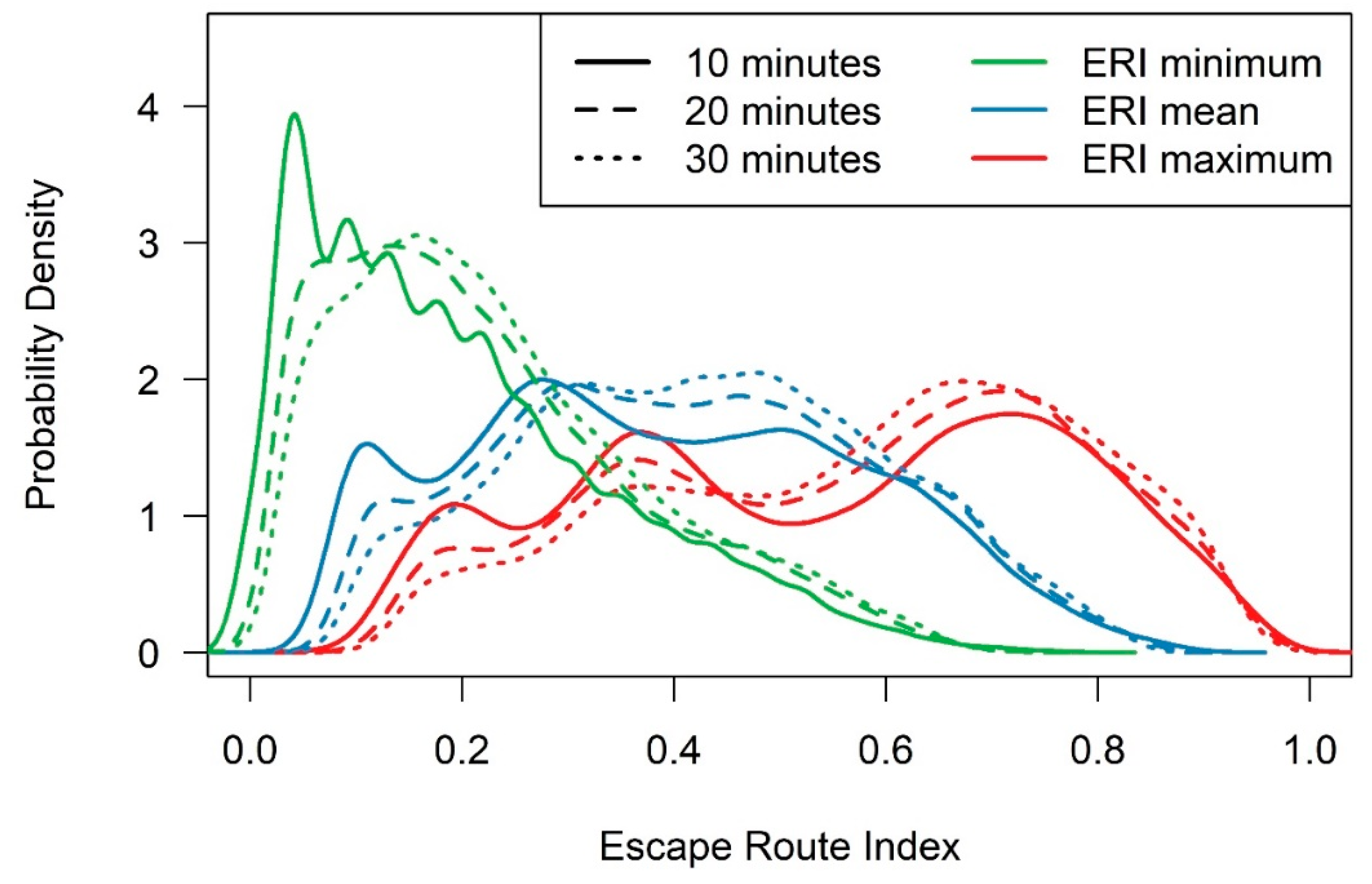Figure 11j)). However, these results should be interpreted with caution for a few important reasons: (1) the mapped land cover conditions represent pre-fire conditions, and do not reflect the degree to which the fires had altered the cover (i.e., travel in the “black” can be substantially faster); (2) it is impossible to determine on a case-by-case scenario the temporal accuracy of the roads and trails—some may have existed pre-fire, but some may have been developed during or after the fire; (3) the ERI does not include any information on the spatial extent of the fire at the time of evacuation, which has perhaps the most important effect on evacuation direction; and (4) although some of the travel distances mapped are larger than others, and as such suggest greater egress capacity, the ERI values across the board are still quite low (Figure 12). For example, for the 30-min evacuation simulations, the mean ERI_min across all incidents was 0.21, the mean ERI_max across all incidents was 0.64, and the mean ERI_mean across all incidents was 0.43. The mean ERI values for burnovers with fatalities tended to be lower than the near misses and the burnovers without fatalities.

4. Discussion

ERI is focused on pre-fire terrain and land cover conditions. Accordingly, it does not account for a number of critical variables that can affect a fire crew’s safety planning decision making processes. Perhaps the most important variable not considered by ERI is the fire extent and growth trajectory. ERI makes the naïve assumption that travel is not restricted in any direction by any factors other than slope and land cover. In reality, fire crews may have 50% or more of potential evacuation directions cut off by the fire itself. Thus, ERI is not a real-time product, as it does not reflect real-time conditions making it a pre-fire decision support tool.

Another important consideration not included in the ERI modeling process is the presence of safety zones. LCES is not a sequence of four disparate safety measures, it is an integrated system of four inherently interdependent safety measures. If no suitable safety zone is accessible from the fireline, then no escape route, regardless of how efficient, is going to be of value. This could be remedied in the future by incorporating ERI maps with maps of existing safety zones, such as those mapped using lidar [26,27]. However, safety zones are often designated “in the black”—in areas that have already burned [28]. As in the case of the fire extent, the dynamism of the fire environment and the associated evolving presence of safety zones is not accounted for in ERI.

Other important safety factors not directly incorporated into ERI are: (1) situational awareness; and (2) potential for snag hazard. Regarding the first exclusion, one could potentially model situational awareness, at least in terms of the ability to perceive surrounding conditions through a GIS-driven viewshed analysis. It is likely that ERI and a terrain-driven viewshed analysis would be highly correlated, since, for example a narrow canyon with limited visibility would also have low egress capacity and vice versa. Regarding the second exclusion, snags act as a significant hazard to wildland firefighters, and thus it is suggested that ERI be used in conjunction with a snag hazard map [29].

Although critical, safety is but one component of the complex, multifaceted wildland fire decision making process [30]. For example, fire crews should also consider the relative potential for suppression effectiveness, incorporating the suppression difficulty index into control location establishment [31]. Accordingly, we are suggesting that ERI become integrated into existing decision support systems, such as WFDSS—particularly since WFDSS data play such a critical role in the formulation of ERI [32]. It is important to distinguish between the existing WFDSS ground evacuation map product and ERI. Although the same land cover travel impedance coefficients are used in both, the end goals of the two products are distinct. WFDSS evacuation maps provide fire managers with a map of the estimated time it would take someone to evacuate to the nearest hospital, and as such, necessarily takes into account the distance to hospitals and automotive travel along a road network. In addition, relatively coarse slope categories are used to model travel impedance. The resulting product is a map of absolute travel time. ERI maps, on the other hand, provide fire managers with a map of relative egress capacity from anywhere in a wildland environment, regardless of proximity to a hospital, and are thusly focused more on evacuation from the fireline to a safety zone than to a health care facility. Additionally, a more precise slope-travel rate function is used as a basis of travel impedance. The output maps either provide a relative safety index, ranging from 0 to 1, or a suggested travel direction.

In its current formulation, based on its current input parameters and datasets, ERI clearly demonstrates a strong influence from land cover—a much greater influence than that of slope. While a previous study has likewise concluded that land cover (in particular, the density of vegetation) can have a stronger effect than slope on travel rates [8], the magnitude of the relative land cover effects derived from WFDSS in this study are very dominant (Figure 10; Table 8). When compared to the few previous studies who have tested the effects of land cover on travel rates, the WFDSS-based effects are the strongest. Given the sparseness of experimental data on the effects of land cover on travel rates, it is unclear which among the few studies, have produced the most reliable results. WFDSS was chosen in this study due to its reliance on existing nationwide data and its wide use in the wildland fire community, but future research may reveal different, more accurate land cover conductance values that should be incorporated into future iterations of ERI.

Another limitation of the WFDSS-driven approach is the fact that, in reality, tree-dominated land cover types are not universally more difficult to traverse than shrub-dominated land cover types. For example, one can move through a mature ponderosa pine parkland environment with a sparse understory, even though it is technically “tree-dominated”, much more readily than one can move through a “shrub-dominated” chaparral environment, such as is present in ANF. This may explain some of the surprising results of the comparison to recent firefighter entrapment events. For example, our evaluation highlighted the fact that the starting point of the escape route that the Granite Mountain Hotshots took possessed a relatively high ERI value, even though their evacuation resulted in one the most significant fatality events in the history of wildland firefighting. This may be due, in part, to the fact that the LANDFIRE EVT data classified the pre-fire land cover for that area as being “shrub-dominated”, thus having a much higher travel conductance than other events. However, according to the Yarnell Hill Serious Accident Investigation Report, “the dominant vegetation type, chaparral brush, ranged in height from one to ten feet and, in some places, was nearly impenetrable” [33].

To overcome the limitations imposed by using categorical land cover types as the basis of travel conductance, we recommend that future research attempt to refine our understanding of how travel rates are affected by more objective, continuous measures of landscape conditions. Because land cover datasets are predominantly derived from passive remote sensing instruments that record reflected solar radiation from the uppermost portions of the Earth’s surface, such as Landsat, they lack the ability to precisely model vertical structure of the landscape. However, active instruments, such as lidar, are capable of making precise x, y, and z measurements, and exploiting small gaps in a vegetated canopy to make measurements of understory vegetation density, which is thought to be a much better predictor of travel conductance [8,34]. With the ever-increasing availability of lidar data in the US, future research should aim to enhance ERI with more precise measures of structurally-based, rather than categorically-based, pedestrian travel conductance.

5. Conclusions

In this paper, we have introduced a new metric for assessing and mapping egress capacity, or the degree to which one can evacuate from a given location, on a broad, spatial scale based on existing landscape conditions. ERI is not a single metric, but a suite of four spatially-explicit metrics that define the relative travel impedance caused by terrain and land cover faced by a fire crew, should that fire crew need to evacuate. The intent is that this modeling technique will be employed to aid in wildland firefighter safety operations prior to engaging a fire, acting as a decision support tool. Given that the metric relies on US nationwide, publicly-available datasets, the goal is that ERI metrics would be mapped in advance of fire suppression and used to direct fire crews toward potential control locations with higher capacity for evacuation, thus reducing the potential for injurious or even fatal entrapments. ERI does not map escape routes, per se, it highlights areas that have a greater or lesser capacity for providing efficient escape routes. Areas with high ERI values will likely have an abundance of open, easily-traversable terrain, through which many potential escape routes may exist requiring little alteration of the land cover. Conversely, areas with low ERI values possess some combination of rugged terrain and dense vegetation, thus making the designation of suitable escape routes difficult or even impossible.

We suggest that the four metrics be used as follows. If a single metric is to be used, then ERI_mean should be that metric. It is the best representation of the overall egress capacity for a given location. High ERI_mean values are likely to produce desirable evacuation conditions. However, means are simply a measure of central tendency, and do not reflect the directionally-specific evacuation conditions. Thus, if a more nuanced planning process is feasible, it is advisable to use the remaining three metrics in conjunction with ERI_mean. ERI_min provides fire personnel with a sense of the worst-case evacuation scenario based on existing landscape conditions. For example, even with a relatively high ERI_mean, if a crew is backed up against a cliff or other impassable feature ERI_min will be very low. In wildland firefighting, where risk levels are high and threats abound, conservative safety planning, such as is offered by ERI_min may be advisable. ERI_mean and ERI_min being equal, a crew might want to know what areas to target for suppression based on the best-case evacuation scenario. This is where ERI_max and ERI_azimuth come into play. A high ERI_max value tells a fire crew that there is at least one direction by which pedestrian evacuation travel efficiency will be very high. ERI_azimuth tells that same fire crew which direction, generally, to take.

References

1. National Wildfire Coordinating Group Glossary A-Z | NWCG. Available online: https://www.nwcg.gov/glossary/a-z (accessed on 17 February 2017).
2. Gleason, P. Lookouts, Communications, Escape Routes, and Safety Zones. Available online: https://www.fireleadership.gov/toolbox/documents/lces_gleason.html (accessed on 17 February 2017).
3. Firefighting Orders and Watch Out Situations (U.S. National Park Service). Available online: https://www.nps.gov/articles/firefighting-orders-watchout-situations.htm (accessed on 28 May 2019).
4. National Wildfire Coordinating Group. Incident Response Pocket Guide; 2018. Available online: https://www.nwcg.gov/sites/default/files/publications/pms461.pdf (accessed on 7 July 2019).
5. Beighley, M. Beyond the safety zone: Creating a margin of safety. Fire Manag. Notes 1995, 55, 21–24. [Google Scholar]
6. Pyne, S.J. Introduction to Wildland Fire, 2nd ed.; Wiley: New York, NY, USA, 1996; ISBN 978-0-471-54913-0. [Google Scholar]
7. Fujioka, F.M.; Gill, A.M.; Viegas, D.X.; Wotton, B.M. Fire danger and fire behavior modeling systems in Australia, Europe, and North America. Dev. Environ. Sci. 2008, 8, 471–498. [Google Scholar]
8. Campbell, M.J.; Dennison, P.E.; Butler, B.W. A LiDAR-based analysis of the effects of slope, vegetation density, and ground surface roughness on travel rates for wildland firefighter escape route mapping. Int. J. Wildland Fire 2017, 26, 884–895. [Google Scholar] [CrossRef]
9. Naismith, W. Cruach Adran, Stobinian, and Ben More. Scott. Mt. Club J. 1892, 2, 136. [Google Scholar]
10. Tobler, W. Three Presentations on Geographical Analysis and Modeling; National Center for Geographic Information and Analysis: Santa Barbara, CA, USA, 1993; p. 24. [Google Scholar]
11. Campbell, M.J.; Dennison, P.E.; Butler, B.W.; Page, W.G. Using crowdsourced fitness tracker data to model the relationship between slope and travel rates. Appl. Geogr. 2019, 106, 93–107. [Google Scholar] [CrossRef]
12. Sugarbaker, L.J.; Eldridge, D.F.; Jason, A.L.; Lukas, V.; Saghy, D.L.; Stoker, J.M.; Thunen, D.R. Status of the 3D Elevation Program, 2015; Open-File Report; U.S. Geological Survey: Reston, VA, USA, 2017.
13. Fryer, G.K.; Dennison, P.E.; Cova, T.J. Wildland firefighter entrapment avoidance: modelling evacuation triggers. Int. J. Wildland Fire 2013, 22, 883–893. [Google Scholar] [CrossRef]
14. Richmond, P.W.; Potter, A.W.; Santee, W.R. Terrain Factors for Predicting Walking and Load Carriage Energy Costs: Review and Refinement. J. Sport Hum. Perform. 2015, 3, 1–26. [Google Scholar]
15. Soule, R.G.; Goldman, R.F. Terrain coefficients for energy cost prediction. J. Appl. Physiol. 1972, 32, 706–708. [Google Scholar] [CrossRef] [PubMed]
16. Pandolf, K.B.; Givoni, B.; Goldman, R.F. Predicting energy expenditure with loads while standing or walking very slowly. J. Appl. Physiol. 1977, 43, 577–581. [Google Scholar] [CrossRef] [PubMed]
17. Alexander, M.E.; Baxter, G.J.; Dakin, G.R. Travel rates of Alberta wildland firefighters using escape routes. In Proceedings of the Human Factors—10 Years Later; Butler, B.W., Alexander, M.E., Eds.; International Association of Wildland Fire: Missoula, MT, USA, 2005. [Google Scholar]
18. Wildland Fire Decision Support System WFDSS Help | Estimated Ground Medevac Time. Available online: https://wfdss.usgs.gov/wfdss_help/WFDSSHelp_Est_Grd_Medevac_Time.html (accessed on 28 May 2019).
19. Escape Routes 2 | NWCG. Available online: https://www.nwcg.gov/committee/6mfs/escape-routes2 (accessed on 28 May 2019).
20. R Core Team. R: A Language and Environment for Statistical Computing; R Foundation for Statistical Computing: Vienna, Austria, 2018. [Google Scholar]
21. Van Etten, J. gdistance: Distances and Routes on Geographical Grids. 2018. Available online: https://cran.r-project.org/web/packages/gdistance/ (accessed on 7 July 2019).
22. Page, W.; Freeborn, P.; Butler, B.; Jolly, W. A review of US wildland firefighter entrapments: trends, important environmental factors and research needs. Int. J. Wildland Fire 2019. [Google Scholar] [CrossRef]
23. Escape Routes 1 (Take 5@2) | NWCG. Available online: https://www.nwcg.gov/committee/6mfs/escape-routes1 (accessed on 6 June 2019).
24. Dijkstra, E.W. A note on two problems in connexion with graphs. Numer. Math. 1959, 1, 269–271. [Google Scholar] [CrossRef] [Green Version]
25. Groemping, U.; Matthias, L. relaimpo: Relative Importance of Regressors in Linear Models. 2018. Available online: https://cran.r-project.org/web/packages/relaimpo/ (accessed on 7 July 2019).
26. Campbell, M.J.; Dennison, P.E.; Butler, B.W. Safe separation distance score: A new metric for evaluating wildland firefighter safety zones using lidar. Int. J. Geogr. Inf. Sci. 2017, 31, 1448–1466. [Google Scholar] [CrossRef]
27. Dennison, P.E.; Fryer, G.K.; Cova, T.J. Identification of firefighter safety zones using lidar. Environ. Model. Softw. 2014, 59, 91–97. [Google Scholar] [CrossRef]
28. Safety Zones 1 (LCES) | NWCG. Available online: https://www.nwcg.gov/committee/6mfs/safety-zones1-lces (accessed on 7 June 2019).
29. Dunn, C.J.; O’Connor, C.D.; Reilly, M.J.; Calkin, D.E.; Thompson, M.P. Spatial and temporal assessment of responder exposure to snag hazards in post-fire environments. For. Ecol. Manag. 2019, 441, 202–214. [Google Scholar] [CrossRef]
30. Thompson, M.P.; y Silva, F.R.; Calkin, D.E.; Hand, M.S. A review of challenges to determining and demonstrating efficiency of large fire management. Int. J. Wildland Fire 2017, 26, 562–573. [Google Scholar] [CrossRef] [Green Version]
31. y Silva, F.R.; Martínez, J.R.M.; González-Cabán, A. A methodology for determining operational priorities for prevention and suppression of wildland fires. Int. J. Wildland Fire 2014, 23, 544–554. [Google Scholar] [CrossRef]
32. Calkin, D.E.; Thompson, M.P.; Finney, M.A.; Hyde, K.D. A Real-Time Risk Assessment Tool Supporting Wildland Fire Decisionmaking. J. For. 2011, 109, 274–280. [Google Scholar]
33. Arizona State Forestry Division. Yarnell Hill Fire: Serious Accident Investigation Report. 2013. Available online: https://wildfiretoday.com/documents/Yarnell_Hill_Fire_report.pdf (accessed on 7 July 2019).
34. Campbell, M.J.; Dennison, P.E.; Hudak, A.T.; Parham, L.M.; Butler, B.W. Quantifying understory vegetation density using small-footprint airborne lidar. Remote Sens. Environ. 2018, 215, 330–342. [Google Scholar] [CrossRef]
Figure 1. The concept of the Margin of Safety adapted from Beighley [5]. T1 represents the time required for the fire to reach a safety zone and T2 is the time required for firefighter(s) (FF) to reach the same safety zone. In order to create a Margin of Safety T1 should exceed T2.
Fire 02 00040 g001
Figure 2. The effects of terrain slope on pedestrian travel rates by WFDSS land cover class.
Fire 02 00040 g002
Figure 3. Study area map showing WFDSS land cover classes derived from the 30m LANDFIRE Existing Vegetation Type (EVT) dataset.
Fire 02 00040 g003
Figure 4. Spatial depiction of Escape Route Index (ERI) modeling technique: (a) sample starting point within the Angeles National Forest (ANF); (b) input spatial datasets for ERI calculation, including elevation and LANDFIRE-derived land cover; (c) accumulated travel time modeled from the starting point with a 30-min threshold applied; and (d) comparison of actual 30-min travel distance to optimal 30-min travel distance, with distance calculations.
Fire 02 00040 g004
Figure 5. Raster geographic information systems (GIS) simulated travel directions (gray arrows) from a starting point (white circle) in (a) four directions, (b) eight directions, and (c) 16 directions, and the resulting polygon shapes representing the optimal travel distance (black lines).
Fire 02 00040 g005
Figure 6. Results of ERI modeling for ERImin, ERImax, ERImean, and ERIazimuth, for each of the three time frames tested (10, 20, and 30 min) throughout the entirety of the ANF.
Fire 02 00040 g006
Figure 7. Probability densities of ERI metric raster cell values for each of the time frames tested throughout the ANF.
Fire 02 00040 g007
Figure 8. The relationship between ERImax and ERImin for a 30-min evacuation time frame, where the red line represents a log-linear regression model, and the black dotted line represents a 1:1 relationship between ERImax and ERImin.
Fire 02 00040 g008
Figure 9. The effects of evacuation time simulation on ERI values (30 vs. 10 min) for (a) ERImax; (b) ERImin; and (c) ERImean.
Fire 02 00040 g009
Figure 10. Large-scale maps containing the two model input datasets (a) elevation, roads/trails, and (b) land cover as well as model output datasets (c) ERImin, (d) ERImax, (e) ERImean, and (f) ERIazimuth.
Fire 02 00040 g010
Figure 11. Simulated travel time results from several recent wildland firefighter entrapment incidents used as the basis for ERI evaluation: (a) Cramer (2003); (b) Little Venus (2006); (c) Panther (2008); (d) Horseshoe 2 (2011); (e) Holloway (2012); (f) Yarnell (2013); (g) King (2014); (h) Liberty (2017); (i) Preacher (2017); (j) Horse Park (2018); and (k) Ranch (2018).
Fire 02 00040 g011
Figure 12. ERImin, ERImax, and ERImean values modeled from the evacuation starting locations for several recent wildland firefighter entrapment incidents.
Fire 02 00040 g012