Moisture Sorption Models for Fuel Beds of Standing Dead Grass in Alaska


Bureau of Land Management, Alaska Fire Service, 1541 Gaffney Road, Fort Wainwright, AK 99703, USA
Fire 2019, 2(1), 2; https://doi.org/10.3390/fire2010002
Submission received: 5 November 2018
/
Revised: 19 December 2018
/
Accepted: 20 December 2018
/
Published: 23 December 2018
Abstract
:Sorption models were developed to predict the moisture content in fuelbeds of standing dead grass from ambient weather measurements. Intuition suggests that the response time of standing dead grass to diurnal changes in weather is negligible and that moisture content tracks the equilibrium moisture content under most field conditions. This assumption suggests that moisture content could be modelled by empirically fitting coefficients to equations of equilibrium moisture content using field measurements. Here, six equations commonly used in wildland fire management and other industries were fit using 293 measurements of weather and moisture content in standing dead grass from Alaska, U.S.A. Predictors were air temperature and either relative humidity or dewpoint depression. Mean absolute errors of the best three models were approximately 1.16% of moisture content. The models predicted well the moisture content of an independently collected dataset from Canada but less so a set from Australia. The models may be used in wildland fire danger rating and fire behavior prediction systems.
1. Introduction
The moisture content of the fuel bed is an important driver of wildland fire behavior and an integral input to fire behavior prediction and fire danger rating systems. In particular, the moisture content (M) of thermally and sorptively thin fuels with a high ratio of surface area to volume drives attributes of flaming combustion such as ignition probability, flame length, fireline intensity, and rate of spread. These fine dead fuels carry fire across the landscape [1]. Fine dead fuels are also known as one-hour timelag fuels and include dead conifer needles, twigs, forest floor litter, and senescent or cured herbaceous foliage. The timelag indicates the rate at which fuel moisture is exponentially lost (or gained) as it approaches an equilibrium moisture content () [2,3,4,5,6,7,8]. However, for some nominal one-hour fuels the effective timelag may be zero if the ratio of surface area to volume is high enough to allow the rate of internal moisture diffusion to equal or exceed the diurnal rate of change in determined by air temperature and relative humidity [9]. In other words, moisture is supplied to the surface of the fuel faster than the air can take it away. As a result, M resides close to . This negligible response time has been intuitively understood for many decades even if it has been seldom mentioned [10]. For example, McArthur [11,12], Fosberg and Deeming [13], and Cheney and Just [14] modelled moisture content as a table of ambient air temperature and relative humidity. Marsden-Smedley and Catchpole [15] modelled M in Tasmanian buttongrass using an equation by Nelson [16]. And Kidnie et al. [17] and Cruz et al. [18] mention the assumption that moisture content in standing dead grass instantaneously responds to changes in weather. If M is typically close to then it follows that moisture content in standing dead grass fuel beds could be simply modelled by an equation that has been calibrated from empirical data, the aim of this paper.
1.1. Equilibrium Moisture Content Equations
Some extensive introduction to equilibrium moisture content equations is necessary since it is central to the development of the predictive models here. Moreover, there is a much greater selection of equations available from the industries of food engineering, agriculture, and building science than the few that have appeared in the fire management literature would suggest.
An equilibrium in moisture content occurs when the net exchange of moisture between the fuel and the atmosphere is zero under constant temperature and relative humidity for an indefinite period of time [4]. varies more or less linearly with air temperature and sigmoidally with relative humidity. It also depends on the direction of approach; it is higher in the direction of desorption than adsorption, a condition called sorption hysteresis which is greatest in the range of 20–40% relative humidity [19]. The sigmoid shape of the curve with relative humidity is a reflection of changes in sorption energy associated with bipolar water molecules interacting with hydrophilic fuel fibers. There are many evolving theories to explain the physics of moisture sorption and they are more fully discussed elsewhere (e.g., [4,19,20,21,22]).
Many equations have some theoretical basis in the physics of sorption. Halsey [23] proposed a thermodynamic equation to describe sorption in multiple monolayers based on the earlier ‘BET’ model of Brunauer, Emmett, and Teller [24]. Iglesias and Chirife [25] modified Halsey’s equation, replacing his temperature term with a two-coefficient, exponential equation, the practical effect of which is to eliminate the dependency of temperature on the other coefficients [26]. The Modified Halsey Equation is:
where is air temperature () and is relative humidity (%).
Henderson [2] developed an equation based on Gibbs’ thermodynamic sorption equation for use in estimating in various agricultural products. Thompson [27] added a third coefficient to the temperature term [19]. The Modified Henderson Equation is:
Chung and Pfost [28] recognized that the empirically measured relationship of free energy () to ,
could be equated with the free energy change of sorption,
where R is the Ideal Gas Constant, 8.314 , and is absolute temperature (). Setting Equation (3) equal to Equation (4) allows solution of as a function of temperature and relative humidity. The Chung-Pfost Equation is:
Nelson [29] independently derived the same equation and fit coefficients [16] for various wildland fuels measured by Blackmarr [30], Van Wagner [31], and Anderson et al. [32].
Pfost et al. [33] added a third coefficient (c) to Equation (5). Coefficient c may be combined with R allowing temperature to be expressed in degrees centigrade. The Modified Chung-Pfost Equation is:
Several other equations with no physical basis have also been proposed. Oswin [34] published a mathematical series expansion equation based on relative humidity to predict the useful life of water vapor resistant packaging. Chen [26] modified the equation by adding a linear term on temperature to produce isotherms for grains and other agricultural products:
Van Wagner [31] developed an equation to describe in several wildland fuels of Eastern Canada. His equation is currently used globally within the Fire Weather Index (FWI) subsystem of the Canadian Forest Fire Danger Rating System [35,36]. He measured at nine levels at a reference temperature () of 27 . He fit four coefficients (, and d) to the left-most two terms of Equation (8) by manually melding a power function to the lower end of the curve with an exponential function at the higher end [32]. A fifth coefficient (f) was added to adjust from to other temperatures. A sixth coefficient (g) was introduced in the final term by Van Wagner and Pickett [37] to adjust convergence near the origin [6]. The present form of Van Wagner’s equation is thus a cludge of several disparately developed terms and efforts:
A last curve is hinted in a U.S. Forest Service Technical Report [38] in which the authors suggest that moisture content in basswood slats could be fit to dry bulb temperature and the logarithm of dewpoint depression. Although their report was intended to predict M rather than , the resulting curve is sigmoidal with relative humidity and linear with temperature and could be considered an equation:
where is dewpoint temperature ().
The above equations are sigmoidal with relative humidity with inflections at approximately 10 and 70% relative humidity (e.g., Figure 2). At the dry inflection point curves drop rapidly toward the origin. At the humid inflection point curves rise toward the fiber saturation point () [20]. varies with temperature [39] and with the physical structure and chemical composition of each fuel such that knowing is fraught with uncertainty but fire behavior and danger rating systems generally assume . Engelund et al. [22] suggest that can approach 40%.
1.2. Objectives
The primary objective of this paper is to provide predictive models of moisture content in standing dead grass for use in fire danger rating systems, fire behavior prediction, and fireline monitoring. One specific need is in burning military training ranges in Alaska, U.S.A. where an appreciable matted thatch layer does not develop due to repeated burning.
The approach presented here is to empirically calibrate the introduced equations using a dataset of environmental and moisture content measurements. Then the calibrated models are evaluated against similar, independently measured datasets of M collected from Canada and Australia. These datasets provide an opportunity to examine the robustness of the models to other biomes.
A lesser objective of this paper is merely to introduce some equations prevalent in other industries as alternatives to those currently used in wildland fire management systems.
2. Methods
2.1. Model Calibration and Comparison
Standing dead grass was mostly sampled in the spring during prescribed burning. Several containers of dead grass were sealed at each weather measurement for later moisture content determination. Samples were collected near Anchorage, Delta Junction, and Fairbanks, Alaska, between 61 and 65 north latitude. Day length increases from about 15 to 21 during spring burning in late April and May, depending on location. Solar noon is approximately 14:00 local time. Samples were collected at 17 sites over 80 days between 2009–2015, during daylight hours. Additional samples were collected that were not associated with prescribed burning in order to increase the range in time, weather, and season over what occurred during burning. Only dead, overwintered grass that was standing, not matted, and free of frost, dew, or other surface moisture was collected. Samples were opportunistically collected over areas ranging from one to several hundred hectares at each burn or sample event. Dead foliage was collected from several grass clumps at ≥4 from the ground to avoid wicking. On average, 1.4 containers were collected per observation (409 containers). The samples were weighed wet and dried to a stable weight at 100 in a convectional drying oven. Gravimetric water content was calculated as the percent ratio of water weight to oven-dry fuel weight. An average of 17.2 s.d. of oven-dry grass were collected per container. Moisture contents were averaged at each observation (n = 293).
On-site weather data was collected using a Kestrel 3000 Pocket Weather Meter (Nielsen-Kellerman Corporation, Boothwyn, PA, USA) certified to conform to the standards of the U.S. National Institute of Standards and Technology. The meter was periodically recalibrated as necessary. A small number of samples was collected using a standard, fire-issue sling psychrometer which was hand-selected from many such that both bulbs read the same and correct temperature when dry. Weather measurements were collected away from the influence of fire, fully exposed to the sun and wind, and within several meters of the fuel moisture sample point. Observations were made approximately every hour during prescribed burns. Temperature (), dewpoint temperature (‘dewpoint’, ), relative humidity (%), and windspeed () were collected at eye-level for all samples. Windspeed was an average of approximately one minute. As the project matured estimates of cloud cover (%) were also recorded.
Solar radiation () values were associated from nearby automated weather stations. Not all records were assigned solar radiation values because some of the stations were inappropriate or too far away to capture local conditions. Since the station measurements are reported hourly they were linearly interpolated to the actual times of observation. All times are local, daylight saving time.
Nonlinear least-squares regression was used to fit coefficients to Equations (1), (2), (5)–(7) and (9) using the above dataset with predictors of and or . Van Wagner’s six-coefficient equation (Equation (8)) was not used because Pfost et al. [33] found that equations with more than three coefficients did not yield smaller RMSE values. Sorption hysteresis was ignored since it was rarely clear whether fuels were wetting or drying. Marsden-Smedley and Catchpole [15] found that sorption hysteresis was insignificant in their vapor exchange models for buttongrass. While the main emphasis of this paper is to develop models, some other predictors were also analyzed: windspeed, cloud cover, and solar radiation. The logit transformation was applied to cloud cover fraction [40]. All analyses were conducted in R for Scientific Computing [41]. Nonlinear models were fit using the Levenberg-Marquardt algorithm in the minpack.lm package [42]. A square-root transformation was applied to M in all models to improve variance homoscedasticity. Prior to their evaluation a correction for square-root bias in prediction, the Residual Mean Square (RMS), was added to the result [43,44]. RMS is given in Table 2. A significance level of was assumed. Models were fit with the intent to predict M rather than explain any forcing factors. Some explanatory variables were found to be significant but not useful predictors of M and are not reported.
The models were ranked and compared to one another using several performance statistics on the measured versus predicted values of M generally following Cruz et al. [18] and Cruz et al. [45]: Correlation Coefficient (r), Root Mean Squared Error (RMSE), and Mean Absolute Error (MAE). The Median Symmetric Accuracy (MSA) was used as a measure of relative error [46].
2.2. Suitability of the Models to other Biomes
Following calibration, a subset of the best models was tested against two independently measured evaluation datasets from Canada and Southeastern Australia to examine their robustness to other biomes. Models were evaluated using the same performance statistics described above with the addition of Mean Bias Error (MBE).
The Canada dataset was collected by Wotton [47] near Echo Bay, Sault Ste Marie, Ontario, Canada (46.48 north latitude). Fuel loading of mostly Phleum pratense averaged approximately 0.4 . The grass samples were weathered under snowpack. An automated weather station recorded air temperature, relative humidity, windspeed at 10 , and solar radiation. Six samples of approximately 15 dry weight each of standing dead grass were collected at each observation time. Sampling was carried out during daylight hours from 17 to 25 May 2006. In this analysis observations that occurred within 3 of rainfall were discarded, resulting in 54 observations.
The Australia dataset comprises measurements between 2013 and 2016 from five grassland sites in Victoria, New South Wales, and Queensland, Australia [17,18]. The sites ranged in south latitude between 27.5 to 37.5. Three to ten replicate samples of 20–30 each were collected of standing dead grass during daylight hours, mostly before experimental fires. Fuel loads ranged from 0.24 to 0.46 . A weather station recorded air temperature, relative humidity, solar radiation, and windspeed at approximately eye-level. Unlike the Canada dataset the grass cures seasonally but does not over-winter under snow. For the purposes of this paper only samples that were fully cured were included, resulting in 75 observations.
3. Results
3.1. Model Calibration and Comparison
Environmental factors in the Alaska dataset (Appendix A) spanned broad ranges in season, time of day, solar elevation angle, cloud cover, temperature and relative humidity (Table 1, Figure 1). Resulting moisture contents ranged 4–29%, spanning most of the range below the fiber saturation point.
Equations of (with predictors and either or ) best fit the data (Table 2). Addition of solar radiation, cloud cover, and windspeed, singly or in combination, did not significantly improve the models.
Performance of the models seemed to rank in two distinct groups (Table 3). The poorest three models were Modified Halsey, Modified Henderson, and Chung-Pfost. The Modified Henderson showed the greatest RMSE. MAE and MSA were highest for the two-coefficient Chung-Pfost model. The best group of models included Dewpoint Depression, Modified Chung-Pfost, and Modified Oswin. Performance statistics were negligibly different from one another and were markedly better than the other three models, which are no longer discussed. RMSE and MAE were on the order of 1.71% and 1.16%, respectively. These models are depicted in Figure 2. Complete, untransformed equations, corrected for square-root bias in prediction by the RMS, are given in Equations (10)–(12).
Modified Chung-Pfost:
Modified Oswin:
Dewpoint Depression:
3.2. Suitability of the Models to Other Biomes
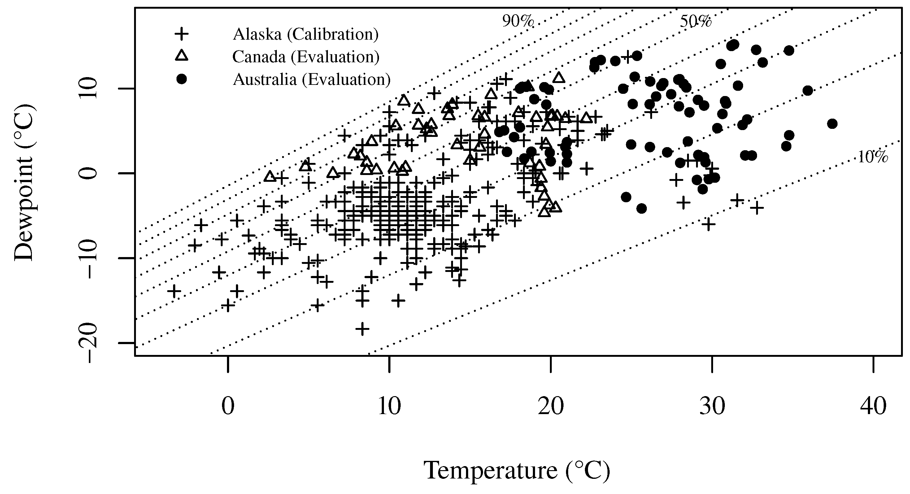
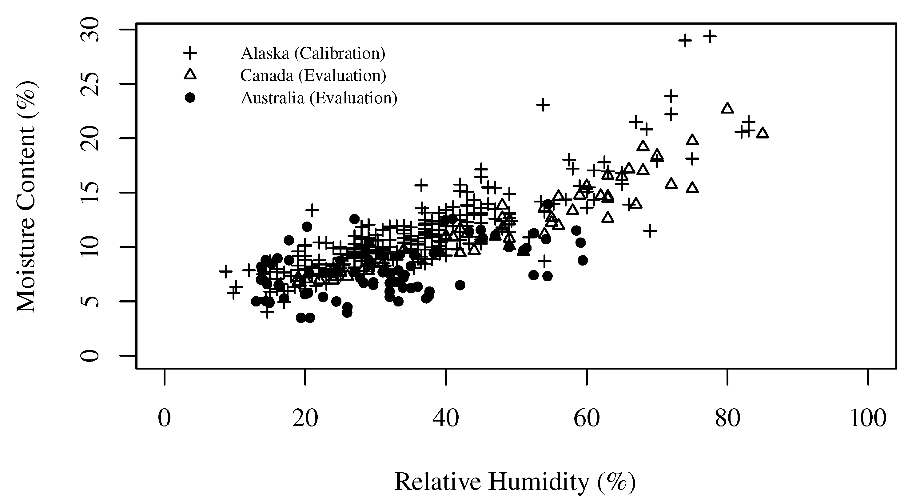
Environmental conditions in the Australia evaluation dataset were quite different from either the Alaska (calibration) or Canada (evaluation) datasets, reflecting gross differences in climate and geographic location (Table 1). The weather variables , , and only weakly overlapped (Figure 1). M was restricted to % or about halfway to the fiber saturation point (Figure 3). The Canada dataset was fairly similar to the Alaska dataset. The ranges of , , and were somewhat narrower but entirely overlapped (Figure 1). M ranged up to 23%.
The Dewpoint Depression, Modified Chung-Pfost, and Modified Oswin models performed well against the Canada dataset. Remarkably, r and RMSE were slightly better against the Canada dataset than against the models’ own calibration dataset (Compare Table 3 with Table 4). MAE and MSA were only slightly poorer. The models yielded lower correlation and higher error against the Australia dataset. Some consistent overprediction bias (MBE) was evident against both datasets.
4. Discussion
4.1. Model Calibration and Comparison
In the falling rate drying period (drying below the fiber saturation point) M should be dependent on internal rather than external processes [3]. The internal processes of sorption and diffusion should be influenced by solar radiation and cloud cover, which determine, in part, fuel temperature, but not by windspeed. As expected, windspeed was not significant. However, contrary to expectation, solar radiation and cloud cover were also not significant. After removing the effects of and or the residuals showed no pattern when plotted against solar radiation or cloud cover. Wotton [47] also found no effect of solar radiation on M in standing dead grass fuelbeds although it was a significant contributor to his model for matted grass. Marsden-Smedley and Catchpole [15] found that aspect was not significant in their model for buttongrass, a finding they suggested was due to weak forcing by solar radiation. These results suggest that gains in heat and temperature from solar radiation are quickly lost to the environment in the sorptively and thermally thin, vertically-oriented standing dead grass fuel bed.
Moisture content was best predicted using equations with predictors of and or , confirming the intuitive importance of these atmospheric drivers of moisture content in fine dead fuels. Performance of the six models varied somewhat but all of the models fit the data well, providing compelling evidence that M is close to over the range of sampled environmental conditions.
Models based on equations with three-coefficients performed better than the model based on the two-coefficient Chung-Pfost equation more familiarly known in the field of fire science as Nelson’s Equation [16,29]. Nelson’s Equation has been useful in developing equations for various fuels in the past because these experimental efforts typically fix the air temperature at a single reference value and manipulate the relative humidity. However, when using field measurements that vary broadly in temperature to predict M, a third coefficient on improves accuracy [25].
Of the best three models there is little basis for selection except on the convenience of predictor, relative humidity or dewpoint depression.
4.2. Suitability of the Models to other Biomes
The models appear to be best suited to temperate and boreal North American grasslands. The models predicted the Canada dataset well, no doubt following from similarities in the fuel bed and climate. Both regions are characterized by grasses that are similar in architecture and loading, and that weather under a snowpack. In essence, the models performed well because they were asked to predict values of M from a test dataset that was similar to the calibration dataset.
Performance was poorer against the Australia dataset. The spread of M with relative humidity in the Australia dataset was more cloud-like than that of either the Canada or Alaska datasets, partly because M ranges to only 14%, about half that of the Alaska dataset and only about halfway to the fiber saturation point. In comparison to six fine dead or grass moisture content models tested against the same Australia dataset by Cruz et al. (Table 3 from [18]), RMSE and MAE of the Alaska models ranked in the middle and were only slightly poorer than the best models, suggesting that variance in M limits other models as well. It also suggests that the Alaska models may not be wholly unsuited for use in Australian grasslands.
Some diminishment in their performance could be expected from extrapolation of the models outside their calibration domain, specifically, to higher temperatures and dewpoints in the Australia dataset, and to a fuel bed that seasonally senesces but does not weather under a snowpack. Senescence may result in differences in physical structure or chemistry that affect the availability of sorption sites or the rate of internal bulk diffusion. Van Wagner [48] and Anderson [5] have demonstrated that weathering results in differences in response time and , respectively, but the specific effects of curing or senecescence remain speculative.
Some consistent, positive bias (MBE) in prediction occurred against both evaluation datasets. Analysis of residuals suggests the bias stems from humidity more than temperature, pointing to differences in sensors. Electronic humidity sensors are typically more variable than temperature sensors and is unfortunately more sensitive to than to .
5. Conclusions
Equilibrium moisture content equations, most from other industries and rarely used in wildland fire science applications, produced sound models of moisture content in standing dead grass. The performance of the models presented here confirms the intuition that M below the fiber saturation point remains predictably close to under most daytime field conditions and that M can be reliably predicted from temperature and either relative humidity or dewpoint depression. Solar radiation and cloud cover were not significant predictors, suggesting that standing dead grass is too thermally thin to retain gains in solar heat. The three best models performed well against an independently measured dataset from Canada, suggesting they are suited to boreal and temperate North American grasslands where winter snowpacks occur. Suitability for Australian grasslands is less confident.
Funding
This research was funded by the U.S. Bureau of Land Management, Alaska Fire Service.
Acknowledgments
Many people contributed data, logistics, code, discussions, and reviews: Mike Wotton (Canadian Forest Service), Miguel Cruz (CSIRO, Canberra, ACT, Australia), Susan Kidnie (Country Fire Authority, Fire and Emergency Management, Australia), Matt Jolly (U.S. Forest Service, Rocky Mountain Research station), Kent Slaughter, Tami Defries, Jake Dollard, and Dan Rees. The Alaska Resources Library and Information Service was indispensible to the literature review.
Conflicts of Interest
The author declares no conflict of interest. The funder had no role in the design of the study; in the collection, analyses, or interpretation of data; in the writing of the manuscript, or in the decision to publish the results.
Abbreviations
The following abbreviations are used in this manuscript:
| Solar elevation angle () | |
| CC | Cloud cover (%) |
| Free energy () | |
| Relative Humidity (%) | |
| MAE | Mean absolute error (Units of of M) |
| MBE | Mean bias error (Units of of M) |
| MSA | Median Symmetric Accuracy (%) |
| M | Moisture content (%) |
| Moisture content, equilibrium (%) | |
| Moisture content, fiber saturation point (%) | |
| r | Correlation coefficient |
| R | Ideal Gas Constant (8.314 ) |
| RMS | Residual Mean Square |
| RMSE | Root mean squared error (Units of of M) |
| Air temperature, () | |
| Dewpoint temperature () | |
| Air Temperature, () | |
| Air temperature, reference () | |
| Wind speed, eye-level () |
Appendix A

Table A1.
Alaska Dataset Used for Model Calibration.
| Site | Date & Time | () | () | (%) | () | () | CC (%) | M (%) |
|---|---|---|---|---|---|---|---|---|
| G | 2009-05-05 10:30 | 10.6 | 3.9 | 62 | 0.9 | 38 | 17.8 | |
| G | 2009-05-05 11:30 | 12.2 | 4.4 | 59 | 1.2 | 43 | 15.6 | |
| G | 2009-05-05 14:00 | 13.3 | 1.7 | 45 | 0.9 | 44 | 13.6 | |
| G | 2009-05-05 15:00 | 14.4 | 4.4 | 52 | 1.3 | 40 | 10.9 | |
| SMR | 2009-05-16 12:45 | 13.3 | −8.3 | 21 | 44 | 13.4 | ||
| SMR | 2009-05-16 14:45 | 14.4 | −8.3 | 20 | 40 | 10.2 | ||
| SMR | 2009-05-16 16:30 | 14.7 | −8.6 | 19 | 32 | 8.3 | ||
| SMR | 2009-05-16 17:00 | 14.4 | −8.9 | 19 | 29 | 9.6 | ||
| SMR | 2009-05-16 19:00 | 13.9 | −8.9 | 20 | 16 | 9.2 | ||
| CL | 2010-04-16 14:15 | 5.0 | −10.6 | 32 | 34 | 11.9 | ||
| D | 2010-04-17 11:50 | 11.1 | −7.2 | 29 | 1.3 | 35 | 12.1 | |
| D | 2010-04-17 12:40 | 12.2 | −6.7 | 29 | 0.9 | 36 | 9.7 | |
| HDZ | 2010-04-17 14:30 | 12.8 | −5.0 | 29 | 1.3 | 33 | 9.0 | |
| HDZ | 2010-04-17 16:15 | 13.3 | −6.1 | 25 | 1.8 | 25 | 8.3 | |
| CL | 2010-04-18 13:20 | 18.9 | −3.3 | 22 | 0.4 | 36 | 10.4 | |
| WR | 2010-04-20 12:05 | 8.3 | −13.9 | 20 | 37 | 8.0 | ||
| WR | 2010-04-20 15:00 | 8.3 | −15.0 | 17 | 2.0 | 32 | 7.7 | |
| WR | 2010-04-20 17:45 | 10.6 | −15.0 | 15 | 1.3 | 17 | 8.7 | |
| BAX | 2010-04-23 13:00 | 5.6 | −15.6 | 19 | 1.8 | 39 | 9.2 | |
| BAX | 2010-04-23 15:00 | 8.3 | −18.3 | 14 | 2.7 | 33 | 7.5 | |
| SMR | 2010-04-24 13:30 | 8.3 | −7.8 | 31 | 1.8 | 38 | 11.6 | |
| SMR | 2010-04-24 13:54 | 9.4 | −7.8 | 27 | 37 | 9.8 | ||
| SMR | 2010-04-24 14:45 | 9.4 | −10.0 | 25 | 1.3 | 35 | 9.8 | |
| SMR | 2010-04-24 15:50 | 11.1 | −8.9 | 24 | 30 | 9.9 | ||
| SMR | 2010-04-24 17:25 | 11.1 | −10.6 | 20 | 0.7 | 21 | 10.1 | |
| SMR | 2010-04-24 18:30 | 8.9 | −12.2 | 20 | 1.3 | 14 | 8.8 | |
| MPTR | 2010-05-03 13:30 | 11.7 | −1.1 | 37 | 1.8 | 44 | 0 | 12.5 |
| MPTR | 2010-05-03 14:20 | 12.8 | −1.1 | 35 | 1.2 | 42 | 0 | 10.3 |
| MPTR | 2010-05-03 15:20 | 16.1 | −1.7 | 29 | 1.2 | 38 | 0 | 9.7 |
| MPTR | 2010-05-03 16:20 | 15.0 | −2.2 | 31 | 2.8 | 32 | 0 | 9.8 |
| MPTR | 2010-05-03 19:30 | 13.9 | −2.8 | 30 | 1.3 | 10 | 0 | 10.6 |
| MPTR | 2010-05-03 20:30 | 15.0 | −2.8 | 31 | 3 | 9.9 | ||
| G | 2010-05-04 10:30 | 9.4 | −3.9 | 39 | 1.1 | 38 | 0 | 11.6 |
| G | 2010-05-04 11:25 | 10.6 | −3.3 | 38 | 0.7 | 42 | 0 | 11.2 |
| G | 2010-05-04 12:20 | 11.7 | −2.8 | 35 | 1.6 | 44 | 0 | 9.6 |
| G | 2010-05-04 16:45 | 15.0 | −2.2 | 31 | 2.7 | 30 | 0 | 9.3 |
| G | 2010-05-04 19:15 | 13.9 | −3.3 | 29 | 1.9 | 12 | 9.5 | |
| M | 2010-05-05 10:40 | 13.3 | −3.3 | 35 | 0.4 | 39 | 11.8 | |
| M | 2010-05-05 11:10 | 10.6 | −2.2 | 38 | 41 | 12.4 | ||
| M | 2010-05-05 11:55 | 12.2 | −2.8 | 37 | 1.2 | 44 | 12.0 | |
| CL | 2010-05-20 10:00 | 15.0 | 3.9 | 47 | 1.0 | 38 | 95 | 12.6 |
| CL | 2010-05-20 12:30 | 15.6 | 6.1 | 48 | 0.6 | 45 | 95 | 11.8 |
| CL | 2010-05-20 14:17 | 18.3 | 7.2 | 45 | 1.5 | 43 | 95 | 10.3 |
| CL | 2010-05-20 15:55 | 17.8 | 6.1 | 45 | 1.5 | 36 | 10.5 | |
| WR | 2011-04-23 11:45 | 9.4 | −6.1 | 32 | 3.6 | 38 | 10.0 | |
| WR | 2011-04-23 12:30 | 10.0 | −6.1 | 32 | 4.0 | 39 | 11.8 | |
| WR | 2011-04-23 13:21 | 10.6 | −6.1 | 30 | 3.3 | 38 | 90 | 10.0 |
| WR | 2011-04-23 15:45 | 13.3 | −5.6 | 26 | 3.4 | 30 | 25 | 9.2 |
| WR | 2011-04-23 17:15 | 13.9 | −6.1 | 25 | 2.1 | 21 | 20 | 9.8 |
| WR | 2011-04-24 13:30 | 12.2 | −6.7 | 25 | 2.3 | 38 | 0 | 9.0 |
| WR | 2011-04-24 15:30 | 12.8 | −5.6 | 25 | 1.9 | 31 | 0 | 9.9 |
| BAX | 2011-04-25 14:30 | 12.2 | −5.0 | 29 | 2.0 | 36 | 70 | 10.1 |
| BAX | 2011-04-25 17:00 | 11.7 | −6.7 | 28 | 2.7 | 23 | 60 | 9.1 |
| BAX | 2011-04-26 11:20 | 10.6 | −6.1 | 30 | 1.1 | 38 | 10 | 11.1 |
| BAX | 2011-04-26 12:45 | 11.7 | −5.6 | 27 | 1.7 | 40 | 20 | 10.3 |
| BAX | 2011-04-26 13:48 | 12.2 | −6.1 | 27 | 2.4 | 38 | 20 | 9.6 |
| BAX | 2011-04-27 10:30 | 5.0 | −1.1 | 61 | 1.4 | 35 | 17.0 | |
| BAX | 2011-04-29 12:45 | 10.0 | −5.6 | 34 | 2.8 | 41 | 35 | 11.6 |
| BAX | 2011-04-29 13:45 | 10.6 | −5.0 | 33 | 2.2 | 39 | 35 | 9.4 |
| BAX | 2011-04-29 16:10 | 10.6 | −5.0 | 31 | 1.9 | 29 | 75 | 10.0 |
| BAX | 2011-04-29 17:30 | 10.6 | −5.6 | 31 | 3.4 | 21 | 75 | 9.7 |
| BAX | 2011-04-29 18:30 | 11.1 | −5.0 | 31 | 3.8 | 14 | 25 | 9.4 |
| BAX | 2011-04-29 19:30 | 11.7 | −5.0 | 31 | 1.2 | 8 | 20 | 9.8 |
| BAX | 2011-04-30 09:55 | 7.8 | −5.0 | 40 | 1.1 | 33 | 100 | 12.5 |
| BAX | 2011-04-30 11:30 | 9.4 | −5.0 | 34 | 1.9 | 39 | 100 | 11.2 |
| BAX | 2011-04-30 12:30 | 11.1 | −6.1 | 31 | 3.3 | 41 | 100 | 9.5 |
| BAX | 2011-04-30 13:30 | 11.7 | −5.6 | 30 | 3.4 | 40 | 100 | 9.7 |
| BAX | 2011-04-30 14:45 | 11.1 | −5.6 | 30 | 4.5 | 36 | 100 | 8.9 |
| BAX | 2011-04-30 15:45 | 10.0 | −6.1 | 31 | 3.3 | 32 | 100 | 8.2 |
| BAX | 2011-04-30 17:00 | 9.4 | −6.7 | 31 | 3.6 | 24 | 100 | 9.1 |
| BAX | 2011-05-01 11:35 | 8.9 | −5.0 | 36 | 1.1 | 40 | 40 | 10.2 |
| BAX | 2011-05-01 12:20 | 11.7 | −4.4 | 30 | 0.4 | 41 | 35 | 9.4 |
| BAX | 2011-05-01 13:30 | 10.0 | −6.7 | 28 | 1.5 | 40 | 45 | 9.2 |
| BAX | 2011-05-01 14:35 | 8.3 | −1.7 | 49 | 3.2 | 37 | 70 | 11.4 |
| D | 2011-05-03 13:00 | 7.2 | −2.2 | 46 | 2.4 | 41 | 60 | 15.5 |
| D | 2011-05-03 14:00 | 8.3 | −3.9 | 40 | 2.1 | 39 | 60 | 13.4 |
| D | 2011-05-03 15:00 | 10.0 | −2.8 | 37 | 2.4 | 36 | 60 | 11.7 |
| CTR | 2011-05-05 11:20 | 9.4 | −5.6 | 34 | 0.5 | 40 | 90 | 11.9 |
| CTR | 2011-05-05 12:30 | 7.2 | −7.8 | 32 | 0.9 | 42 | 75 | 11.8 |
| CTR | 2011-05-05 13:30 | 10.0 | −7.8 | 27 | 1.3 | 42 | 60 | 11.0 |
| SMR | 2011-05-13 11:50 | 6.1 | −6.1 | 40 | 1.2 | 43 | 75 | 11.9 |
| SMR | 2011-05-13 14:00 | 8.3 | −5.0 | 37 | 1.4 | 42 | 100 | 10.8 |
| SMR | 2011-05-13 15:25 | 10.0 | −5.0 | 36 | 1.4 | 37 | 100 | 10.5 |
| SMR | 2011-05-13 16:30 | 8.3 | −5.0 | 37 | 1.7 | 31 | 100 | 10.8 |
| SMR | 2011-05-13 17:30 | 9.4 | −4.4 | 37 | 0.8 | 25 | 100 | 12.2 |
| SMR | 2011-05-13 18:45 | 10.0 | −3.3 | 39 | 1.4 | 17 | 95 | 10.6 |
| SMR | 2011-05-14 11:40 | 13.3 | −3.9 | 30 | 0.8 | 43 | 0 | 9.6 |
| SMR | 2011-05-14 12:30 | 13.9 | −5.0 | 27 | 0.9 | 44 | 0 | 9.1 |
| SMR | 2011-05-14 13:20 | 14.4 | −3.9 | 27 | 0.7 | 44 | 0 | 9.0 |
| SMR | 2011-05-14 14:30 | 14.4 | −4.4 | 26 | 1.5 | 41 | 3 | 9.3 |
| SMR | 2011-05-14 15:45 | 15.6 | −5.0 | 23 | 0.8 | 35 | 5 | 7.9 |
| SMR | 2011-05-14 16:30 | 17.2 | −4.4 | 22 | 2.0 | 31 | 5 | 7.5 |
| SMR | 2011-05-14 17:30 | 17.2 | −5.0 | 22 | 0.6 | 25 | 5 | 8.1 |
| WR | 2012-04-23 12:30 | 10.0 | −1.1 | 43 | 39 | 10 | 15.1 | |
| WR | 2012-04-23 13:34 | 8.9 | −2.8 | 41 | 0.8 | 38 | 10 | 13.7 |
| WR | 2012-04-23 14:14 | 9.4 | −3.9 | 39 | 0.8 | 36 | 12.4 | |
| WR | 2012-04-23 15:05 | 10.6 | −3.9 | 35 | 1.9 | 33 | 15 | 11.1 |
| WR | 2012-04-23 16:04 | 11.7 | −3.9 | 32 | 0.5 | 28 | 15 | 10.7 |
| CTR | 2012-04-24 13:30 | 9.4 | −4.4 | 37 | 2.4 | 39 | 20 | 8.5 |
| CTR | 2012-04-24 15:01 | 11.1 | −5.6 | 28 | 1.3 | 34 | 30 | 11.9 |
| CTR | 2012-04-24 15:55 | 11.1 | −6.7 | 25 | 1.1 | 29 | 30 | 7.4 |
| CTR | 2012-04-24 17:00 | 8.9 | −4.4 | 38 | 1.8 | 23 | 100 | 10.9 |
| CTR | 2012-04-25 13:25 | 10.6 | −4.4 | 34 | 2.0 | 39 | 40 | 10.4 |
| CTR | 2012-04-25 15:15 | 9.4 | −1.7 | 44 | 1.2 | 33 | 50 | 13.2 |
| CTR | 2012-04-25 16:30 | 9.4 | −3.3 | 39 | 1.6 | 26 | 40 | 10.1 |
| D | 2012-04-28 11:07 | 10.6 | −3.9 | 36 | 0.5 | 37 | 10.3 | |
| D | 2012-04-28 11:42 | 10.6 | −3.9 | 35 | 39 | 40 | 10.7 | |
| D | 2012-04-28 12:27 | 11.7 | −3.9 | 30 | 0.8 | 40 | 50 | 8.9 |
| D | 2012-04-28 13:17 | 12.2 | −4.4 | 31 | 1.9 | 39 | 35 | 9.9 |
| D | 2012-04-28 13:56 | 11.7 | −4.4 | 31 | 2.0 | 38 | 35 | 8.6 |
| D | 2012-04-28 14:57 | 11.7 | −4.4 | 31 | 1.7 | 35 | 90 | 9.0 |
| D | 2012-04-28 15:53 | 12.2 | −2.2 | 36 | 1.0 | 30 | 60 | 8.9 |
| D | 2012-04-28 16:57 | 11.7 | −2.8 | 33 | 0.7 | 24 | 80 | 9.3 |
| L | 2012-05-01 17:32 | −0.6 | −11.7 | 42 | 3.5 | 22 | 90 | 12.5 |
| BAX | 2012-05-03 11:21 | 1.7 | −9.4 | 43 | 0.9 | 40 | 100 | 13.9 |
| BAX | 2012-05-03 12:13 | 2.2 | −9.4 | 43 | 1.3 | 42 | 100 | 13.8 |
| BAX | 2012-05-03 13:03 | 3.3 | −10.0 | 37 | 2.1 | 42 | 100 | 13.2 |
| BAX | 2012-05-03 13:57 | 4.4 | −8.3 | 37 | 1.6 | 40 | 95 | 11.4 |
| BAX | 2012-05-03 15:12 | 6.7 | −7.2 | 37 | 1.7 | 35 | 95 | 11.2 |
| BAX | 2012-05-03 16:43 | 7.8 | −6.7 | 33 | 1.7 | 27 | 100 | 11.9 |
| BAX | 2012-05-03 17:07 | 7.2 | −6.7 | 35 | 1.7 | 24 | 100 | 11.0 |
| BAX | 2012-05-03 18:10 | 7.2 | −7.2 | 34 | 1.7 | 18 | 100 | 10.8 |
| Y-IPBC | 2012-05-04 11:00 | 5.6 | −6.1 | 42 | 1.0 | 38 | 15 | 15.8 |
| Y-IPBC | 2012-05-04 12:00 | 7.8 | −5.0 | 39 | 1.3 | 41 | 15 | 12.1 |
| Y-IPBC | 2012-05-04 13:18 | 9.4 | −7.8 | 28 | 1.9 | 41 | 20 | 10.0 |
| Y-IPBC | 2012-05-04 14:11 | 10.0 | −7.2 | 28 | 1.0 | 39 | 35 | 10.1 |
| Y-IPBC | 2012-05-04 15:06 | 10.0 | −7.2 | 28 | 0.8 | 36 | 60 | 10.9 |
| BAX | 2012-05-05 11:50 | 8.3 | −3.9 | 40 | 1.1 | 42 | 9.8 | |
| BAX | 2012-05-05 12:40 | 8.3 | −4.4 | 37 | 0.6 | 43 | 35 | 9.8 |
| BAX | 2012-05-05 13:37 | 11.1 | −4.4 | 34 | 1.8 | 42 | 50 | 10.4 |
| BAX | 2012-05-05 16:25 | 12.2 | −5.6 | 29 | 2.5 | 29 | 50 | 9.7 |
| SMR | 2012-05-08 09:40 | 6.1 | −3.3 | 48 | 0.8 | 33 | 50 | 11.8 |
| SMR | 2012-05-08 10:00 | 6.7 | −3.3 | 45 | 0.7 | 35 | 60 | 12.2 |
| SMR | 2012-05-08 12:00 | 11.1 | −2.8 | 40 | 0.7 | 42 | 75 | 11.9 |
| SMR | 2012-05-08 13:00 | 11.1 | −2.2 | 37 | 1.3 | 43 | 95 | 11.1 |
| CL | 2012-05-14 11:10 | 11.7 | −8.9 | 23 | 1.7 | 41 | 5 | 10.4 |
| CL | 2012-05-14 12:03 | 14.4 | −8.3 | 19 | 1.3 | 44 | 10 | 7.9 |
| CL | 2012-05-14 12:52 | 14.4 | −8.9 | 18 | 1.3 | 44 | 10 | 7.3 |
| CL | 2012-05-14 13:26 | 13.9 | −7.8 | 22 | 1.9 | 44 | 10 | 8.8 |
| CL | 2012-05-14 14:05 | 12.8 | −8.9 | 21 | 0.8 | 42 | 15 | 7.3 |
| CL | 2012-05-14 15:02 | 12.8 | −8.3 | 21 | 0.9 | 39 | 20 | 8.2 |
| CL | 2012-05-14 16:32 | 13.9 | −7.8 | 22 | 2.2 | 31 | 20 | 8.4 |
| L | 2012-05-22 16:23 | 22.2 | 0.6 | 25 | 1.2 | 34 | 100 | 7.4 |
| L | 2012-05-23 12:59 | 19.7 | 7.2 | 45 | 0.4 | 46 | 60 | 10.7 |
| L | 2012-05-23 13:12 | 17.2 | 6.1 | 45 | 1.3 | 46 | 60 | 13.0 |
| L | 2012-05-24 11:02 | 16.1 | 7.8 | 57 | 0.5 | 43 | 85 | 14.4 |
| L | 2012-05-24 16:16 | 21.7 | 5.0 | 33 | 0.5 | 35 | 85 | 8.8 |
| L | 2012-05-29 16:36 | 15.0 | 2.8 | 42 | 1.3 | 33 | 70 | 10.7 |
| L | 2012-05-31 15:07 | 20.7 | 0.0 | 26 | 0.6 | 42 | 100 | 8.4 |
| L | 2012-06-01 15:20 | 16.7 | 6.1 | 48 | 0.7 | 41 | 90 | 11.7 |
| L | 2012-06-05 09:31 | 17.2 | 11.1 | 67 | 0.6 | 37 | 15 | 21.5 |
| L | 2012-06-08 15:46 | 24.8 | 13.7 | 49 | 0.6 | 39 | 90 | 12.4 |
| L | 2012-06-20 15:00 | 26.2 | 7.2 | 30 | 0.5 | 44 | 10 | 8.2 |
| ED | 2013-04-20 09:35 | 0.0 | −15.6 | 29 | 0.0 | 27 | 0 | 10.2 |
| ED | 2013-04-20 13:30 | 6.1 | −12.8 | 23 | 0.8 | 36 | 0 | 8.0 |
| ED | 2013-04-20 16:30 | 5.6 | −12.2 | 25 | 0.6 | 25 | 0 | 7.8 |
| ED | 2013-04-22 08:58 | −3.3 | −13.9 | 43 | 0.0 | 25 | 0 | 11.9 |
| ED | 2013-04-23 20:15 | 5.6 | −10.3 | 31 | 0.0 | 3 | 100 | 8.5 |
| ED | 2013-05-02 20:05 | 1.9 | −8.9 | 39 | 0.0 | 6 | 70 | 13.2 |
| ED | 2013-05-03 19:33 | 0.6 | −5.6 | 65 | 0.7 | 10 | 100 | 16.8 |
| ED | 2013-05-03 20:25 | −1.7 | −6.1 | 70 | 0.6 | 5 | 100 | 17.9 |
| ED | 2013-05-04 11:40 | −2.1 | −8.5 | 60 | 0.4 | 40 | 100 | 15.5 |
| ED | 2013-05-04 14:32 | 1.3 | −7.3 | 55 | 0.3 | 38 | 100 | 14.0 |
| ED | 2013-05-04 18:29 | 3.3 | −6.7 | 49 | 0.5 | 17 | 80 | 13.1 |
| ED | 2013-05-04 21:40 | −0.4 | −7.8 | 54 | 0.0 | -1 | 0 | 8.7 |
| ED | 2013-05-05 11:00 | 2.8 | −10.0 | 40 | 0.3 | 38 | 0 | 9.2 |
| ED | 2013-05-05 14:02 | 2.2 | −11.7 | 35 | 0.3 | 40 | 0 | 9.8 |
| ED | 2013-05-05 19:50 | 3.9 | −7.8 | 40 | 0.4 | 9 | 0 | 9.2 |
| ED | 2013-05-17 08:26 | 2.2 | −3.9 | 60 | 0.5 | 28 | 100 | 15.1 |
| ED | 2013-05-17 16:51 | 3.3 | −5.6 | 49 | 0.4 | 30 | 100 | 13.2 |
| ED | 2013-05-18 17:07 | 0.6 | −13.9 | 33 | 0.4 | 28 | 0 | 9.6 |
| ED | 2013-05-18 17:13 | 16.7 | 10.6 | 69 | 0.0 | 28 | 0 | 11.5 |
| BAX | 2013-05-21 12:03 | 11.7 | −10.0 | 21 | 0.5 | 46 | 0 | 8.1 |
| BAX | 2013-05-21 13:03 | 11.7 | −13.1 | 16 | 2.7 | 46 | 3 | 8.0 |
| BAX | 2013-05-21 13:22 | 12.2 | −11.7 | 16 | 2.0 | 46 | 3 | 6.1 |
| BAX | 2013-05-21 13:30 | 13.9 | −11.5 | 15 | 1.2 | 46 | 3 | 7.1 |
| BAX | 2013-05-21 13:55 | 13.9 | −11.1 | 15 | 1.6 | 45 | 3 | 7.7 |
| BAX | 2013-05-21 14:28 | 14.3 | −12.6 | 14 | 0.6 | 43 | 5 | 7.1 |
| BAX | 2013-05-21 14:57 | 14.4 | −10.0 | 16 | 0.4 | 41 | 3 | 6.6 |
| BAX | 2013-05-21 15:27 | 14.4 | −11.3 | 16 | 1.4 | 38 | 3 | 7.1 |
| BAX | 2013-05-21 16:02 | 15.3 | −7.2 | 22 | 2.5 | 35 | 3 | 6.5 |
| BAX | 2013-05-21 17:00 | 16.4 | −7.2 | 18 | 0.5 | 29 | 3 | 6.3 |
| BAX | 2013-05-22 11:49 | 16.7 | −3.9 | 23 | 0.4 | 46 | 0 | 7.8 |
| BAX | 2013-05-22 13:03 | 16.7 | −5.6 | 20 | 1.3 | 46 | 0 | 7.2 |
| BAX | 2013-05-22 14:03 | 17.8 | −5.6 | 20 | 1.4 | 44 | 5 | 6.2 |
| BAX | 2013-05-22 15:02 | 16.7 | −5.6 | 23 | 2.8 | 40 | 5 | 6.6 |
| BAX | 2013-05-22 16:05 | 16.1 | −6.7 | 19 | 3.5 | 35 | 5 | 6.5 |
| BAX | 2013-05-22 17:05 | 15.6 | −8.6 | 18 | 3.0 | 29 | 5 | 6.0 |
| G | 2013-05-24 08:35 | 10.0 | 2.2 | 58 | 0.4 | 30 | 0 | 17.2 |
| G | 2013-05-24 11:05 | 14.4 | 3.6 | 49 | 1.1 | 45 | 5 | 12.7 |
| G | 2013-05-24 11:58 | 15.6 | 3.9 | 45 | 0.9 | 48 | 5 | 10.9 |
| G | 2013-05-24 13:00 | 16.1 | 3.6 | 43 | 1.1 | 50 | 2 | 10.3 |
| G | 2013-05-24 15:03 | 19.4 | 3.5 | 33 | 0.5 | 44 | 8 | 9.1 |
| G | 2013-05-24 15:58 | 21.1 | 3.7 | 31 | 0.5 | 39 | 15 | 8.3 |
| G | 2013-05-24 16:55 | 20.8 | 3.3 | 33 | 0.8 | 33 | 20 | 9.2 |
| G | 2013-05-24 17:55 | 21.7 | 3.9 | 32 | 1.3 | 25 | 30 | 8.0 |
| G | 2013-05-25 10:00 | 15.4 | 1.7 | 40 | 0.3 | 40 | 0 | 11.1 |
| G | 2013-05-25 11:05 | 16.1 | 2.2 | 39 | 0.7 | 45 | 1 | 10.4 |
| G | 2013-05-25 12:03 | 16.7 | 3.1 | 38 | 0.7 | 49 | 1 | 10.0 |
| G | 2013-05-25 13:02 | 18.9 | 2.2 | 32 | 0.8 | 50 | 2 | 8.8 |
| G | 2013-05-25 15:33 | 17.9 | 1.1 | 30 | 2.2 | 41 | 2 | 8.3 |
| G | 2013-05-25 16:43 | 19.2 | −1.4 | 24 | 2.9 | 34 | 5 | 7.8 |
| R-IPBC | 2013-05-26 08:50 | 11.1 | 3.9 | 61 | 0.0 | 32 | 98 | 14.4 |
| R-IPBC | 2013-05-26 10:46 | 10.0 | 3.3 | 66 | 1.6 | 44 | 85 | 13.9 |
| R-IPBC | 2013-05-26 11:47 | 11.4 | 3.3 | 54 | 1.0 | 48 | 70 | 14.2 |
| R-IPBC | 2013-05-26 14:00 | 19.1 | 0.3 | 30 | 0.9 | 48 | 60 | 10.6 |
| R-IPBC | 2013-05-26 15:03 | 16.4 | 3.1 | 36 | 1.1 | 44 | 80 | 9.1 |
| R-IPBC | 2013-05-26 16:10 | 18.3 | 3.9 | 38 | 0.4 | 38 | 80 | 8.9 |
| MPTR | 2013-05-27 16:22 | 23.5 | 5.0 | 29 | 1.2 | 37 | 1 | 8.2 |
| MPTR | 2013-05-27 16:28 | 23.2 | 4.6 | 28 | 1.2 | 36 | 1 | 7.8 |
| MPTR | 2013-05-27 16:44 | 23.3 | 4.6 | 28 | 1.0 | 34 | 1 | 7.5 |
| ED | 2013-05-29 16:33 | 29.1 | 1.5 | 17 | 0.4 | 34 | 3 | 4.9 |
| ED | 2013-05-29 16:38 | 29.9 | −0.2 | 15 | 0.3 | 33 | 3 | 4.0 |
| L | 2013-05-30 15:14 | 28.5 | 1.5 | 17 | 0.7 | 41 | 8 | 6.0 |
| L | 2013-05-30 15:19 | 30.0 | 0.6 | 15 | 0.7 | 41 | 8 | 5.9 |
| L | 2013-05-30 15:24 | 27.8 | -0.8 | 14 | 0.9 | 40 | 8 | 5.3 |
| ED | 2013-06-05 08:03 | 10.0 | 5.6 | 75 | 0.3 | 28 | 100 | 18.1 |
| ED | 2013-06-05 10:38 | 9.4 | 4.4 | 72 | 0.5 | 43 | 100 | 22.2 |
| ED | 2013-06-05 14:08 | 10.0 | 7.2 | 83 | 0.0 | 46 | 100 | 21.5 |
| ED | 2013-06-05 16:01 | 12.8 | 9.4 | 83 | 0.0 | 38 | 100 | 20.7 |
| WR | 2014-04-15 12:36 | 8.3 | −1.7 | 49 | 0.5 | 36 | 100 | 14.9 |
| WR | 2014-04-15 13:05 | 8.9 | −2.2 | 46 | 1.7 | 36 | 100 | 14.0 |
| WR | 2014-04-15 13:50 | 8.3 | −2.2 | 46 | 2.1 | 35 | 100 | 15.5 |
| WR | 2014-04-15 15:06 | 9.4 | −2.8 | 43 | 1.8 | 30 | 100 | 12.3 |
| WR | 2014-04-15 16:07 | 10.0 | −2.8 | 39 | 1.2 | 25 | 100 | 13.1 |
| WR | 2014-04-15 17:08 | 8.3 | −2.8 | 43 | 0.8 | 19 | 13.0 | |
| BAX | 2014-04-17 12:06 | 7.2 | 0.0 | 60 | 1.2 | 36 | 30 | 13.6 |
| BAX | 2014-04-17 13:14 | 7.8 | −1.7 | 54 | 2.3 | 36 | 30 | 13.2 |
| BAX | 2014-04-17 14:10 | 8.3 | −1.7 | 47 | 1.8 | 35 | 25 | 13.5 |
| BAX | 2014-04-17 15:08 | 10.0 | −2.8 | 38 | 1.5 | 31 | 20 | 11.5 |
| BAX | 2014-04-17 16:12 | 9.4 | −2.8 | 42 | 3.0 | 25 | 30 | 15.2 |
| BAX | 2014-04-17 17:05 | 8.9 | −2.2 | 43 | 2.9 | 20 | 20 | 12.3 |
| BAX | 2014-04-17 18:13 | 9.4 | −4.4 | 37 | 1.5 | 13 | 15 | 11.4 |
| BAX | 2014-04-17 18:47 | 8.3 | −5.0 | 37 | 2.1 | 9 | 15 | 12.1 |
| BAX | 2014-04-17 19:40 | 7.2 | −3.3 | 45 | 3.1 | 3 | 15 | 13.0 |
| BAX | 2014-04-18 09:10 | 3.3 | −3.3 | 63 | 1.7 | 26 | 25 | 17.0 |
| BAX | 2014-04-19 09:24 | 5.6 | −5.6 | 45 | 0.6 | 27 | 2 | 13.2 |
| BDZ | 2014-04-20 08:55 | 8.3 | −2.8 | 47 | 0.7 | 25 | 0 | 15.5 |
| BDZ | 2014-04-20 09:50 | 7.2 | −4.4 | 42 | 3.5 | 30 | 0 | 12.5 |
| BDZ | 2014-04-20 10:59 | 7.8 | −4.4 | 38 | 3.4 | 35 | 0 | 12.1 |
| BDZ | 2014-04-20 11:26 | 8.3 | −3.9 | 41 | 2.2 | 36 | 0 | 11.9 |
| BDZ | 2014-04-20 12:01 | 10.0 | −4.4 | 35 | 2.5 | 37 | 0 | 10.3 |
| BDZ | 2014-04-20 13:25 | 12.2 | −3.3 | 33 | 2.2 | 37 | 10 | 9.3 |
| BDZ | 2014-04-20 13:58 | 11.7 | −3.3 | 34 | 3.0 | 36 | 10 | 9.7 |
| BDZ | 2014-04-20 16:28 | 11.1 | −6.7 | 27 | 1.3 | 25 | 40 | 9.9 |
| BDZ | 2014-04-20 17:21 | 11.7 | −6.7 | 28 | 0.6 | 19 | 40 | 9.8 |
| BDZ | 2014-04-20 18:45 | 11.1 | −7.2 | 25 | 3.2 | 10 | 40 | 9.3 |
| BDZ | 2014-04-20 19:25 | 10.6 | −7.2 | 27 | 1.9 | 6 | 30 | 9.3 |
| CTR | 2014-04-21 09:00 | 7.2 | −4.4 | 44 | 0.0 | 25 | 0 | 14.3 |
| CTR | 2014-04-21 10:40 | 7.8 | −5.6 | 39 | 0.8 | 34 | 0 | 12.2 |
| CTR | 2014-04-21 13:34 | 12.2 | −5.6 | 28 | 1.6 | 37 | 20 | 11.0 |
| CTR | 2014-04-21 14:55 | 13.9 | −6.1 | 25 | 1.3 | 33 | 35 | 10.0 |
| CTR | 2014-04-21 15:47 | 11.7 | −7.8 | 25 | 1.0 | 29 | 45 | 7.7 |
| CTR | 2014-04-21 16:55 | 12.8 | −5.6 | 27 | 1.3 | 23 | 40 | 8.0 |
| CTR | 2014-04-21 18:00 | 11.7 | −7.2 | 25 | 1.3 | 16 | 60 | 8.1 |
| CTR | 2014-04-21 18:55 | 11.7 | −5.0 | 31 | 1.0 | 10 | 70 | 9.8 |
| CTR | 2014-04-22 08:10 | 3.3 | −6.1 | 45 | 0.3 | 21 | 5 | 17.1 |
| CTR | 2014-04-22 09:44 | 7.2 | −5.6 | 40 | 0.5 | 30 | 5 | 12.8 |
| CTR | 2014-04-22 12:10 | 11.1 | −6.7 | 29 | 1.4 | 38 | 15 | 10.8 |
| CTR | 2014-04-22 14:35 | 12.2 | −5.6 | 28 | 1.9 | 35 | 60 | 10.8 |
| CTR | 2014-04-22 18:00 | 11.7 | −7.8 | 24 | 1.7 | 16 | 75 | 8.4 |
| CTR | 2014-04-22 19:00 | 10.6 | −6.1 | 28 | 1.2 | 9 | 75 | 9.3 |
| CTR | 2014-04-23 08:55 | 3.9 | −7.2 | 45 | 0.4 | 26 | 0 | 16.4 |
| Y-IPBC | 2014-05-01 18:35 | 20.6 | 0.0 | 27 | 0.4 | 15 | 1 | 8.1 |
| ED | 2014-05-04 05:30 | 3.3 | −0.6 | 74 | 0.0 | 7 | 20 | 29.0 |
| ED | 2014-05-04 08:22 | 8.3 | 3.3 | 72 | 0.4 | 24 | 95 | 23.9 |
| SMC | 2014-05-09 08:46 | 9.4 | −1.7 | 43 | 0.5 | 28 | 0 | 12.9 |
| SMC | 2014-05-09 09:35 | 9.4 | −1.1 | 42 | 0.8 | 34 | 1 | 12.9 |
| SMC | 2014-05-09 10:52 | 10.6 | −1.1 | 42 | 2.1 | 41 | 1 | 11.9 |
| SMC | 2014-05-09 12:00 | 13.3 | −0.6 | 38 | 1.3 | 45 | 2 | 11.0 |
| SMC | 2014-05-09 13:06 | 15.0 | 1.1 | 39 | 1.5 | 46 | 2 | 9.8 |
| SMC | 2014-05-09 15:00 | 18.9 | 0.0 | 29 | 1.7 | 41 | 1 | 9.5 |
| SMC | 2014-05-09 15:57 | 18.3 | −0.6 | 28 | 1.3 | 36 | 1 | 8.7 |
| SMC | 2014-05-09 16:50 | 18.9 | −0.6 | 25 | 1.9 | 30 | 2 | 8.9 |
| SMC | 2014-05-09 17:50 | 18.3 | 0.0 | 29 | 1.4 | 23 | 2 | 8.4 |
| SMC | 2014-05-09 19:00 | 18.3 | −2.2 | 25 | 1.3 | 15 | 20 | 8.3 |
| SMC | 2014-05-09 20:00 | 18.3 | −2.2 | 24 | 1.5 | 8 | 15 | 8.3 |
| ED | 2015-05-18 06:55 | 13.9 | −0.3 | 36 | 18 | 0 | 15.7 | |
| ED | 2015-05-19 06:20 | 5.0 | 1.1 | 78 | 0.0 | 15 | 0 | 29.4 |
| ED | 2015-05-19 09:51 | 20.6 | 5.2 | 37 | 36 | 0 | 13.6 | |
| ED | 2015-05-23 16:00 | 31.6 | −3.2 | 10 | 36 | 10 | 6.3 | |
| ED | 2015-05-23 16:10 | 32.8 | −4.1 | 9 | 1.5 | 35 | 10 | 7.8 |
| ED | 2015-05-23 16:15 | 29.8 | −6.0 | 10 | 0.8 | 34 | 10 | 5.8 |
| ED | 2015-05-23 18:30 | 28.2 | −3.4 | 12 | 21 | 7.9 | ||
| ED | 2015-05-26 07:40 | 16.2 | 7.8 | 54 | 0.7 | 25 | 70 | 23.1 |
| ED | 2015-05-27 09:45 | 14.2 | 8.3 | 68 | 37 | 20.8 | ||
| ED | 2015-05-27 09:50 | 15.0 | 8.3 | 65 | 0.0 | 38 | 15.8 | |
| ED | 2015-05-27 10:45 | 17.5 | 8.9 | 58 | 0.0 | 42 | 80 | 18.0 |
| ED | 2015-05-29 06:30 | 7.2 | 4.4 | 82 | 0.0 | 18 | 90 | 20.6 |
Sites: Donnelly Training Area near Delta Junction: BAX = Battle Area Complex, BDZ = Buffalo Drop Zone, CTR = Collective Training Range/Bondsteel, WR = Wills Range Fort Richardson, Anchorage: G = Grezelka, R-IPBC = Infantry Platoon Battle Course, M = Mahon, MPTR = Multi-Purpose Training Range, SMC = Small Arms Complex, Fort Wainwright, Fairbanks: SMR = Small Arms Range, L = Ladd Field, Yukon Training Area near Eielson Air Force Base: D = Digital Multi-Purpose Training Range, HDZ = Husky Drop Zone, Y-IPBC = Infantry Platoon Battle Course, Other sites: CL = Chena Lakes, ED = Ester Dome
References
- Cheney, P.; Sullivan, A. Grassfires: Fuel, Weather and Fire Behaviour, 2nd ed.; CSIRO Publishing: Collingwood, Australia, 2008. [Google Scholar]
- Henderson, S.M. A basic concept of equilibrium moisture content. Agric. Eng. 1952, 33, 29–32. [Google Scholar]
- Van Wagner, C.E. A laboratory study of weather effects on the drying rate of jack pine litter. Can. J. For. Res. 1979, 9, 267–275. [Google Scholar] [CrossRef]
- Skaar, C. Wood-Water Relations; Springer Series in Wood Science; Springer-Verlag: Berlin/Heidelberg, Germany, 1988. [Google Scholar]
- Anderson, H. Predicting Equilibrium Moisture Content of Some Foliar Forest Litter in the Northern Rocky Mountains; Technical Report; Research Paper INT-429; U.S. Forest Service, Intermountain Forest and Range Experiment Station: Ogden, UT, USA, 1990. [Google Scholar]
- Viney, N.R. A review of fine fuel moisture modelling. Int. J. Wildland Fire 1991, 1, 215–234. [Google Scholar] [CrossRef]
- González, A.D.R.; Hidalgo, J.A.V. Modelos de Predicción de la Humedad de los Combustibles Muertos: Fundamentos y Aplicación; Monografías INIA/Serie Forestal; Monografías INIA, Instituto Nacional de Investigación y Tecnología Agraria y Alimentaria: Madrid, España, 2007. [Google Scholar]
- Matthews, S. Dead fuel moisture research: 1991–2012. Int. J. Wildland Fire 2014, 23, 78–92. [Google Scholar] [CrossRef]
- Byram, G.M.; Nelson, R.M. An Analysis of the Drying Process in Forest Fuel Material; Technical Report; e-General Technical Report SRS-200; U.S. Forest Service, Southern Research Station: Asheville, NC, USA, 2015. [Google Scholar]
- Van Wagner, C.E. Comparison of American and Canadian Forest Fire Danger Rating Systems; Technical Report; Information Report PS-X-2; Canadian Forest Service, Petawawa Forest Experiment Station: Chalk River, ON, Canada, 1966. [Google Scholar]
- McArthur, A.G. Fire Danger Rating Tables for Annual Grasslands; Commonwealth of Australia, Forestry and Timber Bureau: Canberra, Australia, 1960. [Google Scholar]
- McArthur, A.G. Weather and Grassland Fire Behaviour; Commonwealth of Australia, Department of National Development, Forestry and Timber Bureau Leaflet 100: Canberra, Australia, 1966. [Google Scholar]
- Fosberg, M.A.; Deeming, J.E. Derivation of the 1- and 10-Hour Timelag Fuel Moisture Calculations for Fire Danger Rating; Technical Report; Research Note RM-207; U.S. Forest Service, Rocky Mountain Forest and Range Experiment Station: Fort Collins, CO, USA, 1971. [Google Scholar]
- Cheney, N.P.; Just, T.E. The Behaviour and Application of Fire in Sugar Cane in Queensland; Commonwealth of Australia Department of Agriculture, Forestry and Timber Bureau, Leaflet 115: Canberra, Australia, 1974. [Google Scholar]
- Marsden-Smedley, J.B.; Catchpole, W.R. Fire modelling in Tasmanian buttongrass moorlands. III. Dead fuel moisture. Int. J. Wildland Fire 2001, 10, 241–253. [Google Scholar] [CrossRef]
- Nelson, R.M. A method for describing equilibrium moisture content of forest fuels. Can. J. For. Res. 1984, 14, 597–600. [Google Scholar] [CrossRef] [Green Version]
- Kidnie, S.A.; Cruz, M.G.; Matthews, S.; Hurley, R.J.; Slijepcevic, A.; Nichols, D.; Gould, J.S. Evaluating dead fuel moisture models for Australian grasslands. In Proceedings of the International Association of Wildland Fire, Melbourne, Australia, 11–15 April 2016. [Google Scholar]
- Cruz, M.G.; Kidnie, S.; Matthews, S.; Hurley, R.J.; Slijepcevic, A.; Nichols, D.; Gould, J.S. Evaluation of the predictive capacity of dead fuel moisture models for Eastern Australia grasslands. Int. J. Wildland Fire 2016, 25, 995–1001. [Google Scholar] [CrossRef]
- Sun, D.; Woods, J.L. The moisture content/relative humidity equilibrium relationship of wheat—A review. Dry. Technol. 1993, 11, 1523–1551. [Google Scholar] [CrossRef]
- Berry, S.L.; Roderick, M.L. Plant–water relations and the fibre saturation point. New Phytol. 2005, 168, 25–37. [Google Scholar] [CrossRef]
- Mujumdar, A.S. Handbook of Industrial Drying, 3rd ed.; CRC Press: London, UK, 2006. [Google Scholar]
- Engelund, E.T.; Thygesen, L.G.; Svensson, S.; Hill, C.A.S. A critical discussion of the physics of wood–water interactions. Wood Sci. Technol. 2013, 47, 141–161. [Google Scholar] [CrossRef]
- Halsey, G. Physical adsorption on non-uniform surfaces. J. Chem. Phys. 1948, 16, 931–937. [Google Scholar] [CrossRef]
- Brunauer, S.; Emmett, P.H.; Teller, E. Adsorption of gases in multimolecular layers. J. Am. Chem. Soc. 1938, 60, 309–319. [Google Scholar] [CrossRef]
- Iglesias, H.A.; Chirife, J. Prediction of the effect of temperature on water sorption isotherms of food material. Int. J. Food Sci. Technol. 1976, 11, 109–116. [Google Scholar] [CrossRef]
- Chen, C.C. Modification of Oswin EMC/EHR equation. J. Agric. Res. China 1990, 39, 367–376. [Google Scholar] [CrossRef]
- Thompson, T.L.; Peart, R.M.; Foster, G.H. Mathematical simulation of corn drying—A new model. Trans. Am. Soc. Agric. Eng. 1968, 11, 582–586. [Google Scholar] [CrossRef]
- Chung, D.S.; Pfost, H.B. Adsorption and desorption of water vapor by cereal grains and their products Part 1: Heat and free energy changes of adsorption and desorption. Trans. Am. Soc. Agric. Eng. 1967, 10, 549–555. [Google Scholar] [CrossRef]
- Nelson, R.M. A model for sorption of water vapor by cellulosic materials. Wood Fiber Sci. 1983, 15, 8–22. [Google Scholar]
- Blackmarr, W.H. Equilibrium Moisture Content of Common Fine Fuels Found in Southeastern Forests; Technical Report; Research Paper SE-74; U.S. Forest Service, Southeastern Forest Experiment Station: Asheville, NC, USA, 1971. [Google Scholar]
- Van Wagner, C.E. Equilibrium Moisture Contents of Some Fine Forest Fuels in Eastern Canada; Technical Report; Information Report PS-X-32; Canadian Forest Service, Petawawa Forest Experiment Station: Chalk River, ON, Canada, 1972. [Google Scholar]
- Anderson, H.; Schuette, R.; Mutch, R. Timelag and Equilibrium Moisture Content of Ponderosa Pine Needles; Technical Report; Research Paper INT-202; U.S. Forest Service, Intermountain Forest and Range Experiment Station: Ogden, UT, USA, 1978. [Google Scholar]
- Pfost, H.B.; Maurer, S.G.; Chung, D.S.; Milliken, G.A. Summarizing and Reporting Equilibrium Moisture Data for Grains; Technical Report; Paper No. 76-3520; American Society of Agricultural Engineers: St. Joseph, MI, USA, 1976. [Google Scholar]
- Oswin, C.R. The kinetics of package life. III. The isotherm. J. Soc. Chem. Ind. 1946, 65, 419–421. [Google Scholar] [CrossRef]
- Van Wagner, C.E. Development and Structure of the Canadian Forest Fire Weather Index System; Technical Report, Forestry Technical Report 35; Canadian Forestry Service: Ottawa, ON, Canada, 1987. [Google Scholar]
- Stocks, B.J.; Lynham, T.J.; Lawson, B.D.; Alexander, M.E.; Van Wagner, C.E.; McAlpine, R.S.; Dube, D.E. The Canadian Forest Fire Danger Rating System: An overview. For. Chron. 1989, 65, 450–457. [Google Scholar] [CrossRef]
- Van Wagner, C.E.; Pickett, T.L. Equations and Fortran IV Program for the 1976 Metric Version of the Forest Fire Weather Index; Technical Report; Information Report PS-X-58; Canadian Forest Service, Petawawa Forest Experiment Station: Chalk River, ON, Canada, 1975. [Google Scholar]
- USFS. Derivation of Spread Phase Tables National Fire-Danger Rating System; Technical Report; United States Forest Service, Division of Fire Control: Washington, DC, USA, 1966. [Google Scholar]
- Stamm, A.J.; Loughborough, W.K. Thermodynamics of the swelling of wood. J. Phys. Chem. 1935, 39, 121–132. [Google Scholar] [CrossRef]
- Warton, D.I.; Hui, F.K.C. The arcsine is asinine: The analysis of proportions in ecology. Ecology 2011, 92, 3–10. [Google Scholar] [CrossRef] [PubMed]
- R Core Team. R: A Language and Environment for Statistical Computing; R Foundation for Statistical Computing: Vienna, Austria, 2017. [Google Scholar]
- Elzhov, T.V.; Mullen, K.M.; Spiess, A.N.; Bolker, B. minpack.lm: R Interface to the Levenberg-Marquardt Nonlinear Least-Squares Algorithm Found in MINPACK, Plus Support for Bounds; R Package Version 1.2-0; R Foundation for Statistical Computing: Vienna, Austria, 2016. [Google Scholar]
- Miller, D.M. Reducing Transformation Bias in Curve Fitting. Am. Stat. 1984, 38, 124–126. [Google Scholar] [CrossRef]
- Gregoire, T.G.; Qi, F.L.; Boudreau, J.; Nelson, R. Regression estimation following the square-root transformation of the response. For. Sci. 2008, 54, 597–606. [Google Scholar] [CrossRef]
- Cruz, M.G.; Gould, J.S.; Alexander, M.E.; Sullivan, A.L.; McCaw, W.L.; Matthews, S. A Guide to Rate of Fire Spread Models for Australian Vegetation; Technical Report; CSIRO Land and Water Flagship: Canberra, Australia; ACT, Australia and Australasian Fire Authorities Council: Melbourne, Australia, 2015. [Google Scholar]
- Morley, S.K.; Brito, T.V.; Welling, D.T. Measures of Model Performance Based on the Log Accuracy Ratio. Space Weather 2018, 16, 69–88. [Google Scholar] [CrossRef]
- Wotton, B.M. A grass moisture model for the Canadian Forest Fire Danger Rating System. In Proceedings of the Eighth Fire and Forest Meteorology Symposium, Kalispell, MT, USA, 12–15 October 2009. [Google Scholar]
- Van Wagner, C.E. Drying rates of some fine forest fuels. Fire Control Notes 1969, 30, 5–12. [Google Scholar]
Figure 1.
Temperature, dewpoint, and relative humidity in the calibration (Alaska) and evaluation (Canada, Australia) datasets. Relative humidity is shown by the dotted lines.
Figure 1.
Temperature, dewpoint, and relative humidity in the calibration (Alaska) and evaluation (Canada, Australia) datasets. Relative humidity is shown by the dotted lines.

Figure 2.
Measured moisture content vs relative humidity. The best three models (Equations (10), (11), and (12)) are shown at 5 (blue lines) and 25 (red lines).
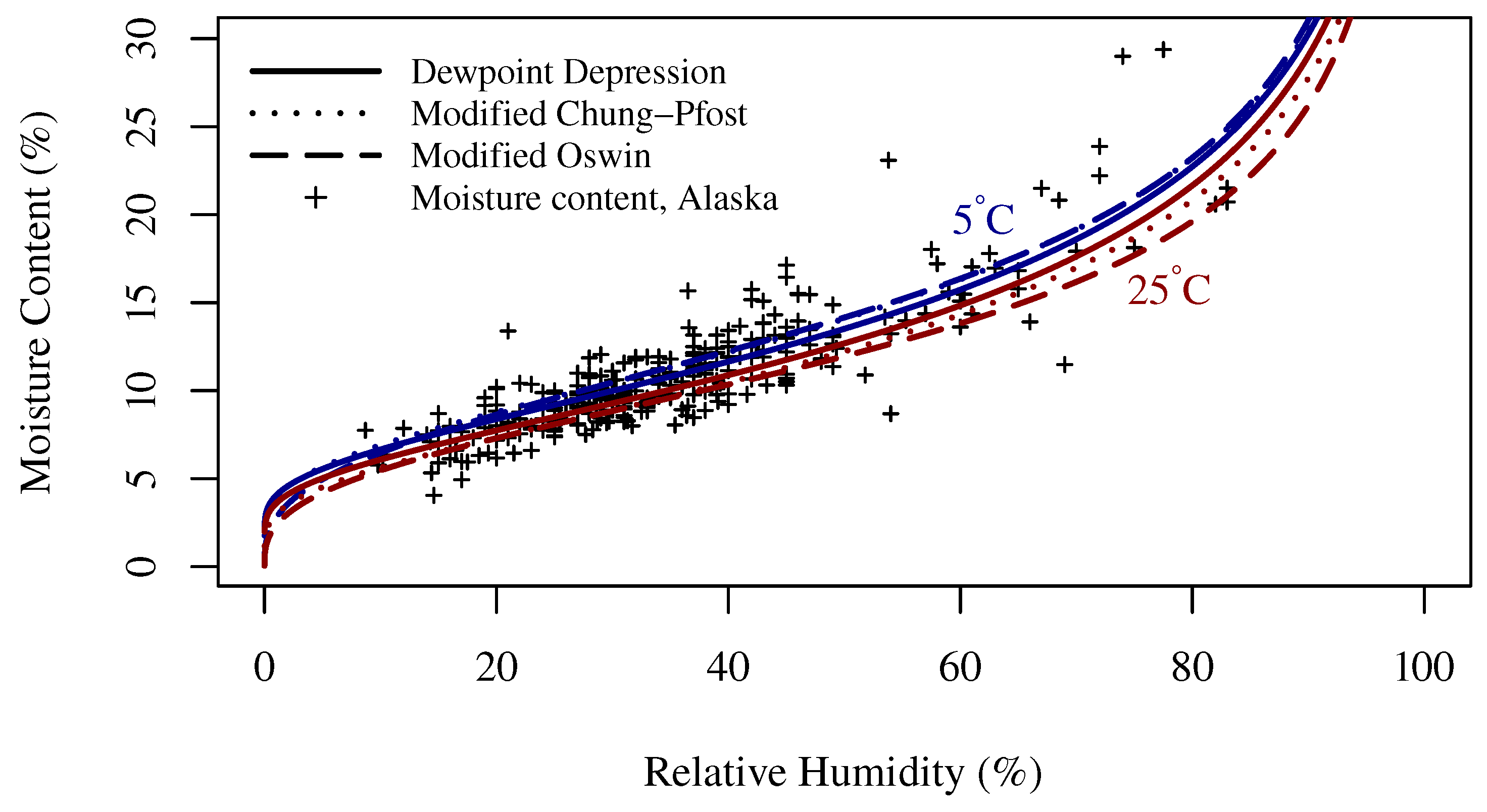
Figure 3.
Moisture content vs relative humidity for the calibration (Alaska) and evaluation (Canada, Australia) datasets.
Figure 3.
Moisture content vs relative humidity for the calibration (Alaska) and evaluation (Canada, Australia) datasets.

Table 1.
Means and ranges of environmental factors for the calibration (Alaska) and evaluation (Canada, Australia) datasets. 137 observations included an estimate of solar radiation.
Table 1.
Means and ranges of environmental factors for the calibration (Alaska) and evaluation (Canada, Australia) datasets. 137 observations included an estimate of solar radiation.
| Region Dataset Type | Alaska Calibration | Canada Evaluation | Australia Evaluation |
|---|---|---|---|
| Day of the Year | 126 (104–171) | 141 (136–144) | 11 (329–116) |
| Time of Day | 14:16 (05:30–21:40) | 14:47 (07:00–21:00) | 13:45 (10:00–19:30) |
| Solar elevation angle () | 33.4 (−1.4–50) | 52.2 (−7.1–65) | |
| Solar radiation () | 474 (0–798) | 449 (11–936) | 756 (53–1392) |
| Temperature ( ) | 12.1 (−3.3–32.8) | 15.1 (2.6–22.2) | 26.3 (16.8–37.5) |
| Dewpoint ( ) | −3.5 (−18.3–13.7) | 3.5 (−4.7–11.2) | 7.3 (−4.1–15.2) |
| Relative humidity (%) | 35.4 (8.7–83) | 49.2 (19–85) | 32.9 (13–59) |
| Windspeed () | 1.3 (0–4.5) | 1.2 (0–2.5) | 2.0 (0.6–4.0) |
| Cloud Cover (%) | 39 (0–100) | ||
| Moisture Content (%) | 11.0 (4.1–29.4) | 12.3 (6.7–22.7) | 8.2 (3.5–13.9) |
| Number of observations | 293 | 54 | 75 |
Table 2.
Regression models. The response variable is . RMS = Residual Mean Square. RSE = Residual Standard Error. d.f. = Degrees of freedom. n = 293.
Table 2.
Regression models. The response variable is . RMS = Residual Mean Square. RSE = Residual Standard Error. d.f. = Degrees of freedom. n = 293.
| Modified Oswin | Modified Halsey | Modified Henderson | Modified hung-Pfost | Chung-Pfost | Dewpoint Depression | |
|---|---|---|---|---|---|---|
| Oswin | Halsey | Henderson | Chung-Pfost | Chung-Pfost | Depression | |
| a | 3.83 *** | 4.86 *** | 64800 *** | *** | ||
| b | *** | *** | ** | *** | *** | * |
| c | *** | *** | *** | *** | *** | |
| RMS | 0.0555 | 0.0566 | 0.0581 | 0.0554 | 0.0581 | 0.0556 |
| RSE | 0.236 | 0.238 | 0.241 | 0.235 | 0.241 | 0.236 |
| d.f. | 290 | 290 | 290 | 290 | 291 | 290 |
*** , ** , * .
Table 3.
Performance statistics of predicted versus measured moisture content for the calibration dataset. r is the correlation coefficient. RMSE is the Root Mean Squared Error. MAE is the Mean Absolute Error. MSA is the Median Symmetrical Accuracy. Models are sorted by RMSE.
Table 3.
Performance statistics of predicted versus measured moisture content for the calibration dataset. r is the correlation coefficient. RMSE is the Root Mean Squared Error. MAE is the Mean Absolute Error. MSA is the Median Symmetrical Accuracy. Models are sorted by RMSE.
| Model | r | RMSE | MAE | MSA (%) |
|---|---|---|---|---|
| Dewpoint Depression | 0.872 | 1.71 | 1.16 | 8.36 |
| Modified Chung-Pfost | 0.871 | 1.71 | 1.16 | 8.64 |
| Modified Oswin | 0.871 | 1.71 | 1.16 | 8.96 |
| Modified Halsey | 0.866 | 1.74 | 1.18 | 8.77 |
| Chung-Pfost | 0.866 | 1.74 | 1.21 | 9.88 |
| Modified Henderson | 0.866 | 1.75 | 1.18 | 9.45 |
Table 4.
Performance of the models against the evaluation datasets from Australia and Canada. Compare with Table 3. MBE is the Mean Bias Error (+Overprediction/−Underprediction).
Table 4.
Performance of the models against the evaluation datasets from Australia and Canada. Compare with Table 3. MBE is the Mean Bias Error (+Overprediction/−Underprediction).
| Model | r | RMSE | MAE | MBE | MSA (%) |
|---|---|---|---|---|---|
| Canada. n = 54 | |||||
| Modified Oswin | 0.956 | 1.66 | 1.26 | +1.15 | 8.76 |
| Dewpoint Depression | 0.953 | 1.69 | 1.23 | +1.12 | 9.08 |
| Modified Chung-Pfost | 0.954 | 1.74 | 1.32 | +1.22 | 9.72 |
| Australia. n = 75 | |||||
| Dewpoint Depression | 0.517 | 2.59 | 2.13 | +1.13 | 23.5 |
| Modified Oswin | 0.513 | 2.61 | 2.17 | +1.20 | 24.8 |
| Modified Chung-Pfost | 0.511 | 2.68 | 2.23 | +1.29 | 26.4 |
© 2018 by the author. Licensee MDPI, Basel, Switzerland. This article is an open access article distributed under the terms and conditions of the Creative Commons Attribution (CC BY) license (http://creativecommons.org/licenses/by/4.0/).
Share and Cite
MDPI and ACS Style
Miller, E.A. Moisture Sorption Models for Fuel Beds of Standing Dead Grass in Alaska. Fire 2019, 2, 2. https://doi.org/10.3390/fire2010002
AMA Style
Miller EA. Moisture Sorption Models for Fuel Beds of Standing Dead Grass in Alaska. Fire. 2019; 2(1):2. https://doi.org/10.3390/fire2010002
Chicago/Turabian StyleMiller, Eric A. 2019. "Moisture Sorption Models for Fuel Beds of Standing Dead Grass in Alaska" Fire 2, no. 1: 2. https://doi.org/10.3390/fire2010002