Multi-Configuration Calculation of Ionization Potential Depression

Abstract

The modelling of ionization potential depression in warm and hot dense plasmas constitutes a real theoretical challenge due to ionic coupling and electron degeneracy effects. In this work, we present a quantum statistical model based on a multi-configuration description of the electronic structure in the framework of Density Functional Theory. We discuss different conceptual issues inherent to the definition of ionization potential depression and compare our results with the famous and widely-used Ecker-Kröll and Stewart-Pyatt models.

1. Introduction

Ionization potentials are fundamental quantities in atomic physics. Their experimental and theoretical studies have aroused the interest of scientists for many years, either for accurate determination [1] or looking for regularities along isoelectronic sequences [2], etc. Ionization potential depression (IPD) or continuum lowering in dense plasmas has been the subject of many investigations over the past years [3,4,5,6]. This many-body effect significantly alters the ionization balance and the corresponding charge state distribution, which have a strong influence on thermodynamic [7], transport [8,9,10] and radiative properties of the system [11,12]. Such a topic is of crucial importance for astrophysics (stellar physics, planetary science, ...) [13,14,15,16], solid state physics and inertial confinement fusion [17,18]. It has an impact on the cross-sections of the different atomic processes, such as collisional excitation or ionization [19,20]. However, an accurate description of IPD in an interactive many-body environment is extremely difficult [21,22,23,24,25,26], because strong correlations and quantum degeneracy have to be taken into account in a consistent manner. Different semi-empirical models have been proposed for the IPD. In particular, the Ecker-Kröll (EK) [27] and the Stewart-Pyatt (SP) model [28] have been widely applied in plasma physics for simulating physical properties and the analysis of experimental measurements. Thanks to the recently developed experimental facilities, it has become possible to explore warm/hot and high-energy density matter, whereby the plasmas are found to be strongly coupled and nearly degenerate. The experimental outcomes can be used to benchmark physical assumptions and theoretical models [19,20]. Over the last few years, new experiments related to the IPD have been performed with high-intense laser beams at LCLS (Linac Coherent Light Source) [29] at SLAC National Accelerator Laboratory [30,31], at ORION in the United Kingdom [32], and at NIF (National Ignition Facility) at Lawrence Livermore National Laboratory [33,34]. Such experiments have revealed the lack of a consistent understanding of IPD, since no satisfying explanation can be drawn for the corresponding measurements using the commonly accepted IPD models (EK and SP). Therefore, a deeper investigation of the IPD in warm/hot dense regime is required. Attempts for a better understanding of the recent experimental data have been made using different models and simulation methods. In particular, two-step Hartree-Fock calculations [35], simulations based on the finite-temperature density functional theory [36,37], classical molecular dynamics simulations [38], and Monte-Carlo simulations [39] have been worked out. Although such outstanding approaches are very successful to explain properties of warm dense matter, they are restricted due to their high computational cost. Besides these simulation methods, other analytic improvements have also been proposed, such as fluctuation model [40], analytic self-consistent approach valid in a wide range of temperatures and densities [41] and atomic-solid-plasma model [42]. The problem of line-shifts in LTE (Local Thermodynamic Equilibrium) plasmas was addressed by Alexiou et al. in the framework of static ions and “active spectator” model. The authors showed that lines can have unshifted (or slightly shifted) peaks with asymmetric tails if the free electron wave functions are strongly localized by the random field of the plasma or by dynamic effects [43] (see in particular the subsection 3.2 entitled “The last bound level”). To emphasize the likely importance of dynamic effects, it is worth quoting the last paragraph of Ref. [44]: “Reading Dick Lee’s comments on the first draft of this paper I realized that, although the work deals with behavior of electrons in a static plasma, the most powerful localization mechanism is dynamic: the finite life-time of a “free” electron. A bound electron becomes “free” when it is kicked out of an ion by a photon, electron, or a collective process. At that time its wave function is still localized at, approximately, the same volume which it had occupied before. Then the wave function begins its time-dependent spread out, and, eventually would have become macroscopic, but, before that happens, the electron is recaptured by an ion, and ends up in another (local) bound state. So, between the time it was “kicked out” and the time it was recaptured it had only a finite period for spreading. This mechanism is unique to a hot matter, where there are enough holes in which the electron can be recaptured”. Very recently, Ren et al. explored the evolution of systems driven to high energy densities using a non-LTE, Fokker-Planck collisional-radiative code. The authors investigated the evolution dynamics of a solid-density plasma driven by an XFEL, and explored the relaxation of the plasma to local thermodynamic equilibrium on femtosecond timescales in terms of the charge state distribution, electron density, and temperature [45]. Motivated by the theoretical as well as experimental challenges related to the understanding of IPD, we present, starting from a quantum statistical theory, a self-consistent multi-configuration approach to IPD. The main idea consists in grouping together (into a so-called superconfiguration) all the configurations representing the excited states of an ion. Therefore, each ion is represented by one single superconfiguration. Then, a self-consistent calculation is carried out for each superconfiguration within the Density Functional Theory (DFT) in the Local Density Approximation (LDA). In such a way, the energies of the subshells and therefore the total energies of the ions, take into account the so-called “density effects” or plasma environment effects. The IPD is obtained as the ionization energy of a given ion from which the “unscreened” value, corresponding to the isolated ion, is subtracted.

Our DFT approach is different from the one used in Ref. [36]. In the latter work, the authors have employed the finite-temperature plane-wave DFT code ABINIT to calculate electron states and energies within a plasma, combined with the projector augmented-wave (PAW) potential formalism used to model a range of different aluminum ions, constructed by creating excited-electron configurations in inner atomic shells and freezing them in the core of the potential. Such a technique belongs to the so-called “ab initio” or molecular-dynamics methods. Our approach is inspired from a different class of models, often referred to as “average-atom models”. The main difference between our approach and usual average-atom models is that we impose an integer number of electrons, in order to deal with a specific ion, in the superconfiguration formalism (the average-atom model provides a mean electronic structure, and therefore fractional numbers of bound electrons, in the different subshells and for the total).

Ecker-Kröll and Stewart-Pyatt analytical models are recalled in Section 2. The self-consistent calculation of electronic structure including screening is presented in Section 3, and the unscreened case in Section 4. The calculation of Ionization Potential Depression is described in Section 5. The results are analyzed in Section 6 and compared to an alternative theoretical approach proposed by Massacrier [46,47,48]. The influence of the temperature on the isolated-atom energy values is discussed, together with the validity of Rayleigh-Schrödinger perturbation theory.

2. Analytical Ionization Potential Depression Models

Let us consider an atom (atomic number Z) which can be partially or totally ionized and k the ionization state ($0\le k\le Z$), having a fraction $F_k$. The ionic density $n_i$ is given by

$$n_i=\frac{\rho {\mathcal{N}}_A}{A},$$

where ${\mathcal{N}}_A$ is the Avogadro number, $\rho$ the matter density (in g/cm³) and A the molar atomic mass (in g). The ionic populations are then $N_k=F_k.n_i$. We define

$${\displaystyle z_1=\frac{{\sum }_{k=0}^{Z}k{F}_k}{n_i}=\frac{n_e}{n_i},}$$

$${\displaystyle z_2=\frac{{\sum }_{k=0}^Z{k}^2{F}_k}{n_i},}$$

and

$$n_i=\sum _{k=0}^Z{N}_k,$$

were $n_e$ represents the electron density. Let us introduce (setting the Boltzmann constant $k_B=1$):

$${\displaystyle z^{*}=\frac{z_2}{z_1}}$$

and

$${\displaystyle {\lambda }_{\mathrm{DH}}=\sqrt{\frac{T}{4\pi n_i\left(z_1+z_2\right)}}=\sqrt{\frac{T}{4\pi n_i{z}_1\left(1+z^{*}\right)}}}$$

the Debye length. For a particle density n (ions, electrons, ions+electrons), we will have to use the modified Debye length

$${\tilde{\lambda }}_{\mathrm{DH}}(n)=\sqrt{\frac{T}{4\pi n}}$$

and the radius

$$R(n)={\left(\frac{3}{4\pi n}\right)}^{1/3}.$$

In particular

$$R_{\mathrm{ws}}=R\left(n_i\right)={\left(\frac{3}{4\pi n_i}\right)}^{1/3}$$

is the Wigner-Seitz radius (i.e., the radius of the average spherical cell representing the average ion) and

$$\begin{array}{ccc}\hfill R\left(n_i+n_e\right)& =& {\left(\frac{3}{4\pi \left(n_i+n_e\right)}\right)}^{1/3}\hfill \\ & =& {\left(\frac{3}{4\pi n_i\left(1+z_1\right)}\right)}^{1/3}=R_{\mathrm{ws}}{\left(1+z_1\right)}^{-1/3}.\hfill \end{array}$$

2.1. Debye-Hückel Model

The expression of the IPD in the Debye-Hückel (DH) theory [49] is

$${\Delta }_{\mathrm{DH}}(i)=\frac{z}{{\lambda }_{\mathrm{DH}}}$$

where i is the charge state and $z=i+1$.

2.2. Stewart-Pyatt Model

The IPD has been formulated in the sixties following two different ways. First, Stewart and Pyatt proposed a model using the finite-temperature potential for the average electrostatic potential near nuclei of the plasma particles [28]. The bound electron are considered as part of the unperturbed ion. The plasma free electrons are described by Fermi-Dirac statistics and ions by Maxwell-Boltzmann statistics. In such a model, the bound electrons do not contribute to the reduction of the ionization energy. The Stewart-Pyatt ionization potential depression is given by [50]:

$${\Delta }_{SP}=\frac{T}{2\left(z^{*}+1\right)}\left\{{\left[\frac{3z\left(z^{*}+1\right)}{{\tilde{\lambda }}_{\mathrm{DH}}(n_i)T}+1\right]}^{2/3}-1\right\}.$$

There are some differences between the understanding and implementation of Stewart-Pyatt model in the literature. Such a point is clarified in Appendix A.

2.3. Ecker-Kröll Model

Second, Ecker and Kröll formulated a generalized Saha equation as a function of the chemical potential of the plasma [27]. This model assumes two different forms for the IPD depending on the particle (ions + electrons) density. Let us introduce the critical density

$$n_c=\frac{3}{4\pi }{\left(\frac{T}{Z^2}\right)}^3,$$

the radius

$$R_{EK}=R\left(n_i+n_e\right)$$

and the constant

$$C_{EK}=\frac{R\left(n_c\right)}{{\tilde{\lambda }}_{\mathrm{DH}}\left(n_c\right)}.$$

If $n_i+n_e\le n_c$, we take (i still represents the charge state):

$$\Delta (i)=\frac{z}{{\tilde{\lambda }}_{\mathrm{DH}}(n_i+n_e)}$$

(1)

and if $n_i+n_e\le n_c$, the EK IPD is provided by

$$\Delta (i)=\frac{C_{EK}z}{R_{EK}},$$

(2)

and the continuity between Equations (1) and (2) is ensured at $n_c$. The dependence of $C_{EK}$ on atomic number Z is discussed in Appendix B.

2.4. Modified Ecker-Kröll Model

Recent experimental results have shown discrepancies with the SP model which is the most widely used among the IPD models and shown good agreement with the EK model version in which $C_{EK}$ has been set to 1 (referred to as “modified EK” model) according to experimental considerations [30]. In contrast, other experimental results obtained independently have corroborated the SP model [32] (see Section 6.1). In the following, we will compare our simulation results with both models SP and EK with $C_{EK}=1$.

3. Self-Consistent Calculations—General Case (Screening of Ions)

A superconfiguration [51,52] is an ensemble of configurations. The superconfiguration approximation consists in partitioning the ensemble of configurations, i.e., in gathering them into groups. A superconfiguration represents a number of configurations of the plasma and is composed by an ensemble of supershells (i.e., groups of subshells) and their respective populations [51,52]. For example, superconfiguration

$$\Xi ={(1s2s2p)}^{10}{(3s3p3d)}^{18}{(4s4p4d4f5s5p5d)}^{19}{(5f5g)}^3$$

represents all the configurations with shells $n=1$, $n=2$ and $n=3$ full, a total of 19 electrons distributed in all possible ways (consistent with the Pauli exclusion principle) in the subshells $4s,4p,4d,4f,5s,5p$ and $5d$ (the third supershell consists of 7 orbitals $4s$ to $5d$), and 3 electrons in the last supershell made of subshells $5f$ and $5g$ only.

In the present work, we have one superconfiguration par ion (which means that all the existing subshells are gathered in the same supershell), and perform therefore one self-consistent calculation of electronic structure per ion.

For a superconfiguration of ionization $Z^{*}$, the electron densities can be adjusted in order to ensure the constraints:

$${\int }_0^{R_{\mathrm{ws}}}4\pi r^2{n}_b(r)dr=Q_b(R_{\mathrm{ws}})=Z-Z^{*}$$

(3)

and

$${\int }_0^{R_{\mathrm{ws}}}4\pi r^2{n}_f(r)dr=Q_f(R_{\mathrm{ws}})=Z^{*},$$

(4)

where $n_e(r)=n_b(r)+n_f(r)$ is the total electron density (bound + free electrons), or, for an average atom

$${\int }_0^{R_{\mathrm{ws}}}4\pi r^2{n}_e(r)dr=Q_e(R_{\mathrm{ws}})=Q_b(R_{\mathrm{ws}})+Q_f(R_{\mathrm{ws}})=Z.$$

(5)

The electron density and the mono-electronic potential are calculated in a self-consistent way in the DFT/LDA theory by an iterative scheme involving Kohn-Sham orbitals and/or Fermi functions. Let k be a bound state, the associated Kohn-Sham mono-electronic orbital obeys the Schrödinger equation (throughout the paper we intentionally omit the “hat” characteristic of quantum-mechanical operators):

$$H{\psi }_k={ϵ}_k{\psi }_k,$$

(6)

H being the Hamiltonian of the system. The mono-electronic potential involved in the definition of H are

$$V_{\mathrm{scf}}(r)=-\frac{Z}{r}+V_e(r)+V_{\mathrm{xc}}\left[n_e(r)\right]$$

where $-Z/r$ is the potential of the nucleus, $V_e(r)$ the potential due to the electrons and $V_{\mathrm{xc}}\left[n_e(r)\right]$ the exchange-correlation potential.

In the nonrelativistic self-consistent spherical ion-cell model, we use the quantum Schrödinger states for free electrons as well as for bound electrons, i.e., the electron number density is obtained by summing over a complete set of bound and free states:

$$n(\overrightarrow{r})=\sum _i{|{\psi }_i(\overrightarrow{r})|}^{2}f({ϵ}_i,\mu )$$

(7)

where f represents the Fermi-Dirac distribution ($\mu$ is the chemical potential, Lagrange multiplier fixing the number of bound electrons of the ion):

$$f({ϵ}_i,\mu )=\frac{1}{1+e^{\left({ϵ}_i-\mu \right)/T}}$$

(8)

and

$${\psi }_i(\overrightarrow{r})=\frac{y_{ϵ,\ell }(r)}{r}{Y}_{\ell }^m(\theta ,\varphi ),$$

(9)

where $Y_{\ell }^m(\theta ,\varphi )$ are the usual spherical harmonics. As the potential is constant outside the ion sphere, the radial wave function of a bound state outside the ion sphere can be written as

$$y_{n\ell }(r)=A_{n\ell }r{\kappa }_{\ell }(-ikr)$$

(10)

where ${\kappa }_{\ell }$ is the modified spherical wave function of the third kind, and the wave vector k is defined as $k=\sqrt{2ϵ}$. The constant $A_{n\ell }$ is determined by the normalization and the boundary conditions at $R_{\mathrm{ws}}$. The condition that the logarithmic derivative of the wave function is continuous at $R_{\mathrm{ws}}$ determines the one-electron eigenvalues $ϵ$. The radial wave function of a free state outside the ion-sphere can be written as

$$y_{ϵ,\ell }(r)=\sqrt{\frac{2k}{\pi }}r\left[cos({\delta }_{ϵ,\ell })j_{\ell }(kr)-sin({\delta }_{ϵ,\ell })n_{\ell }(kr)\right],$$

(11)

where $j_{\ell }$ and $n_{\ell }$ denote spherical Bessel functions of the first and second kinds and ${\delta }_{ϵ,\ell }$ is the phase shift. Shape resonances accompanying the smearing of a bound state in the continuum are taken into account in the density of states [11,53,54]. The bound-electron density then reads

$$n_b(\overrightarrow{r})=\sum _{n,\ell }f({ϵ}_{n\ell },\mu )\frac{2(2\ell +1)}{4\pi }\frac{y_{n\ell }^2(r)}{r^2},$$

(12)

and the free-electron density

$$n_f(\overrightarrow{r})={\int }_0^{\infty }dϵf(ϵ,\mu )\frac{2(2\ell +1)}{4\pi }\frac{y_{ϵ,\ell }^2(r)}{r^2}.$$

(13)

One has to solve, at each iteration of the self-consistent calculation, the Poisson equation, for the determination of the electronic potential

$$V_e(r)=\frac{1}{r}{\int }_0^{r}4\pi r^{\prime 2}{n}_e(r^{\prime })d{r}^{\prime }+{\int }_r^{\infty }4\pi r^{\prime }{n}_e(r^{\prime })d{r}^{\prime }.$$

The total Coulomb potential of the atom (nucleus + electrons) is

$$V_c(r)=-\frac{Z}{r}+V_e(r).$$

We assume that beyond the Wigner-Seitz sphere, the electron charge density is equal to zero, the ionic charges cancelling locally the electron density ($n_e(r)=0$ for $r\ge R_{\mathrm{ws}}$) so that, for $r\ge R_{\mathrm{ws}}$, $V_e(r)=R/r$ and $V_c(r)=0$, because of the conditions (3)–(5).

It is therefore possible to limit ourselves to the calculation of the potential inside the Wigner-Seitz sphere:

$$V_e(r)=\frac{1}{r}{\int }_0^{r}4\pi r^{\prime 2}{n}_e(r^{\prime })d{r}^{\prime }+{\int }_r^{R_{\mathrm{ws}}}4\pi r^{\prime }{n}_e(r^{\prime })d{r}^{\prime },$$

(14)

where

$$V_e(r)=\frac{Q_e(r)}{r}-{\int }_0^r\frac{1}{r^{\prime }}\frac{d{Q}_e}{dr}(r^{\prime })d{r}^{\prime }$$

with

$$Q_e(r)={\int }_0^{r}4\pi r^{\prime 2}{n}_e(r^{\prime })d{r}^{\prime }.$$

Practically, we solve Equation (14) by an inward/backward algorithm (Froese method [55]):

(i)

From $r=0$ to $r=R_{\mathrm{ws}}$: calculation of $Q_e(r)$ by a four-point quadrature formula, the electron density behaving as $r^{\alpha }$ (the value of $\alpha$ is specified in Appendix D) when $r\to 0$.

(ii)

From $r=R_{\mathrm{ws}}$ to $r=0$: calculation of the second term of relation (14) by a four-point quadrature formula.

The mono-electronic energies ${ϵ}_k$, solutions of Schrödinger equation, rely on the assumption that the potential $V_{\mathrm{scf}}$ is equal to zero outside the sphere, which is not the case if the exchange-correlation is non zero, and must therefore be translated from $V_{\mathrm{scf}}(R_{\mathrm{ws}})=V_{\mathrm{xc}}\left[n_e\left(R_{\mathrm{ws}}\right)\right]$.

The self-consistent calculation is initialized by a simple Coulomb potential, and we have seen that the one-electron eigenenergies and wave functions are obtained solving Schrödinger equation. The electron density is built using the latter, the chemical potential is determined by ensuring the integer number of electron in the superconfiguration, the new radial potential is obtained through Poisson’s equation, and the next iteration starts, etc. until convergence. We use a convergence criterion on the central potential, considering that convergence is achieved at iteration n if

$$\underset{0\le r\le R_{\mathrm{ws}}}{max}\left|\frac{V_n(r)-V_{n-1}(r)}{V_{n-1}(r)}\right|\le {10}^{-5}.$$

(15)

4. Self-Consistent Calculations—Unscreened Case

If we impose, for a (super) configuration of ionization $Z^{*}$, the cancellation of the free-electron density $n_f(r)$, one calculates an isolated ion of charge $Z^{*}$, with the occupation constraint

$${\int }_0^{\infty }4\pi r^2{n}_b(r)dr=Q_e(R_{\mathrm{ws}})=Z-Z^{*},$$

where $n_e(r)=n_b(r)$ is the bound-electron density, equal to the total density. The mono-electronic potential involved in the definition of the Hamiltonian H is in that case

$$V_{\mathrm{scf}}(r)=-\frac{Z}{r}+V_b(r)+V_{\mathrm{xc}}\left[n_b(r)\right],$$

where $-Z/r$ is the potential of the nucleus, $V_b(r)$ the potential due to the bound electrons, and $V_{\mathrm{xc}}\left[n_b(r)\right]$ the exchange-correlation potential. As in the screened case, at each iteration, one has to solve the Poisson equation (see Appendix C for the calculation of the electronic potential

$$V_b(r)=\frac{1}{r}{\int }_0^{r}4\pi r^{\prime 2}{n}_b(r^{\prime })d{r}^{\prime }+{\int }_r^{R_{\infty }}4\pi r^{\prime }{n}_b(r^{\prime })d{r}^{\prime },$$

the total Coulomb potential of the isolated ion (nucleus + electrons) still being

$$V_c(r)=-\frac{Z}{r}+V_b(r).$$

We assume that, outside the sphere of radius $R_{\infty }$ (our “numerical infinity), the bound electron density is zero (typically smaller than ${10}^{-7}$ atomic units), the density of the plasma being sufficiently low so that the wave functions (or their derivatives) can be considered as zero $\left(n_b(r)\equiv 0,r\ge R_{\infty }\right)$, so that, for $r\ge R_{\infty }$:

$$V_c(r)=-\frac{Z^{*}}{r}.$$

In practice, $R_{\infty }\approx 10R_{\mathrm{ws}}$, but we always check that the results are not affected if we take a higher value (in the limit of the numerical capabilities of the code, of course). The mono-electronic energies ${ϵ}_k$, solutions of Schrödinger Equation (6), are dependent on the assumption that the potential $V_{\mathrm{scf}}$ is zero outside the sphere, which is not the case, and must be shifted from the quantity

$$V_{\mathrm{scf}}\left(R_{\infty }\right)=-\frac{Z^{*}}{R_{\infty }}+V_{\mathrm{xc}}\left[n_b\left(R_{\infty }\right)\right]=-\frac{Z^{*}}{R_{\infty }}+V_{\mathrm{xc}}(0).$$

5. Calculation of Ionization Potential Depression

5.1. Difference between Screened and Unscreened Energies

Let us consider an isolated (unscreened) ion of average ionization $Z^{*}$. The energy of the mono-electronic Kohn-Sham orbital is ${ϵ}_k+V_{\mathrm{scf}}\left(R_{\infty }\right)$ associated to the wave function ${\psi }_k$ of state k, and solution of Equation (6). The mono-electronic potential entering the definition of the Hamiltonian H is

$$V_{\mathrm{scf}}(r)=-\frac{Z}{r}+V_b(r)+V_{\mathrm{xc}}\left[n_b(r)\right].$$

Let us now consider the screened ion. The energy of the mono-electronic Kohn-Sham orbital is ${\widetilde{ϵ}}_k+{\tilde{V}}_{\mathrm{scf}}\left(R_{\infty }\right)$ associated to the wave function ${\tilde{\psi }}_k$ which obeys $\tilde{H}{\tilde{\psi }}_k={\widetilde{ϵ}}_k{\tilde{\psi }}_k$. The mono-electronic potential entering the Hamiltonian $\tilde{H}$ is

$${\tilde{V}}_{\mathrm{scf}}(r)=-\frac{Z}{r}+{\tilde{V}}_b(r)+{\tilde{V}}_f(r)+{\tilde{V}}_{\mathrm{xc}}\left[{\tilde{n}}_e(r)\right].$$

The ionization potential lowering is, for this bound state

$$\Delta V_k={\widetilde{ϵ}}_k+{\tilde{V}}_{\mathrm{scf}}\left(R_{\mathrm{ws}}\right)-\left[{ϵ}_k+V_{\mathrm{scf}}\left(R_{\infty }\right)\right],$$

i.e.,

$$\Delta V_k=\delta {ϵ}_k+\frac{Z^{*}}{R_{\infty }}+{\tilde{V}}_{\mathrm{scf}}\left(R_{\mathrm{ws}}\right)-V_{\mathrm{scf}}\left(R_{\infty }\right).$$

where $\delta {ϵ}_k={\widetilde{ϵ}}_k-ϵ$. This value can be obtained by subtracting two simulations, one screened and one unscreened.

5.2. First-Order Perturbation Theory

The introduction of a free-electron distribution screening the isolated ion can be understood as a perturbation $\delta H$ of the Hamiltonian of the isolated ion: $H=H_0+\delta H$. The first-order correction to energy reads

$$\langle {\psi }_k|\delta H|{\psi }_k\rangle ,$$

where

$$\delta H=\delta V_{\mathrm{scf}}(r)={\tilde{V}}_f(r)+\delta V_b(r)+\delta V_{\mathrm{xc}}(r)$$

with

$$\delta {\tilde{V}}_{\mathrm{xc}}(r)={\tilde{V}}_{\mathrm{xc}}[{\tilde{n}}_b(r)+{\tilde{n}}_f(r)]-V_{\mathrm{xc}}\left[n_b(r)\right]$$

and $\delta V_b(r)={\tilde{V}}_b(r)-V_b(r)$ denotes the variation of $V_b$ due to the free-electron density. The ionization potential depression reads then, at first order

$$\Delta V_k=\langle {\psi }_k|{\tilde{V}}_f+\delta V_b+\delta V_{\mathrm{xc}}|{\psi }_k\rangle +\frac{Z^{*}}{R_{\infty }}+{\tilde{V}}_{\mathrm{xc}}\left[n_e(R_{\mathrm{ws}})\right]-V_{\mathrm{xc}}\left[n_b(R_{\infty })\right].$$

(16)

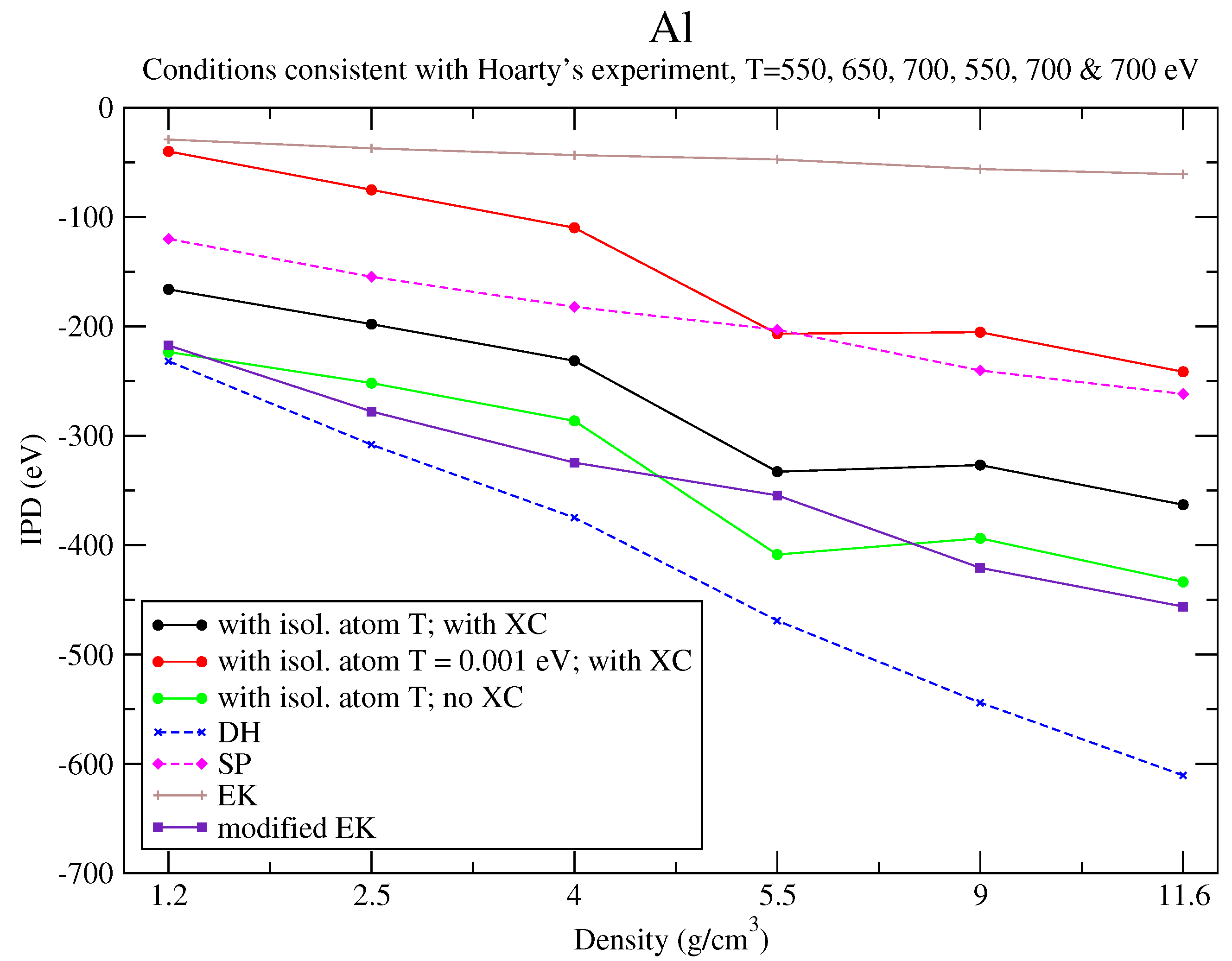
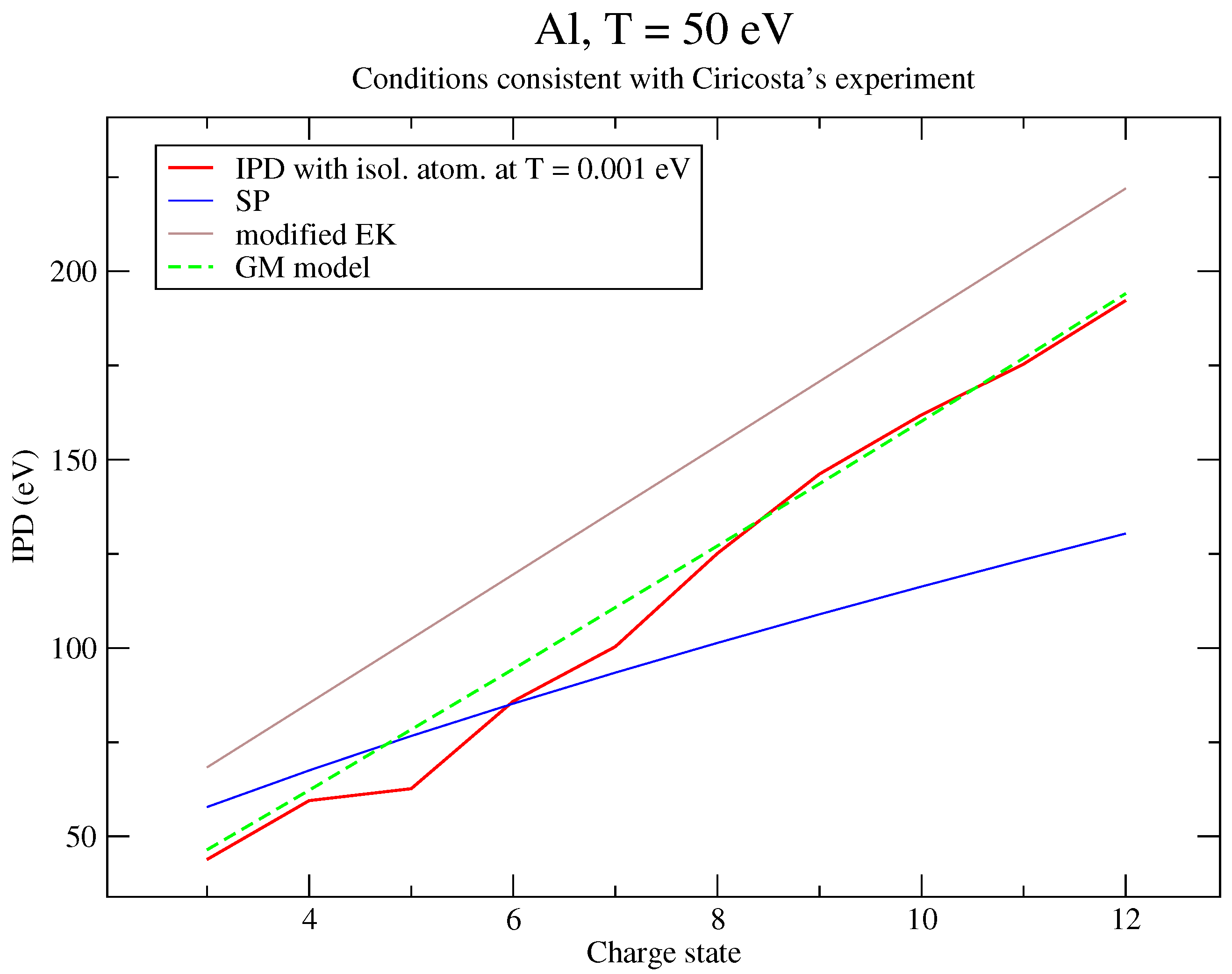
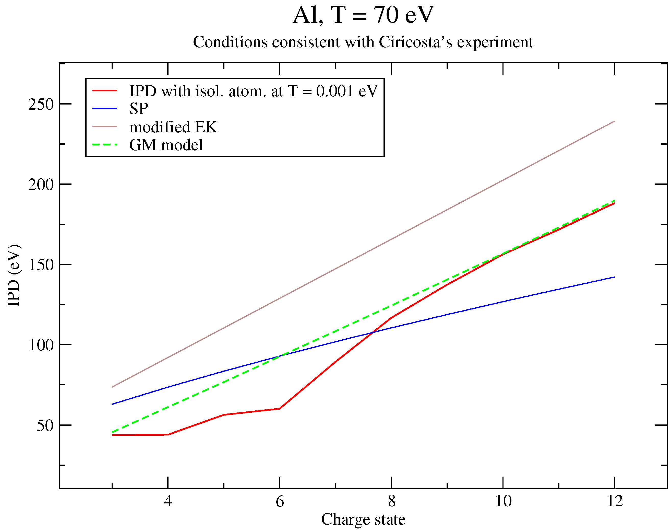
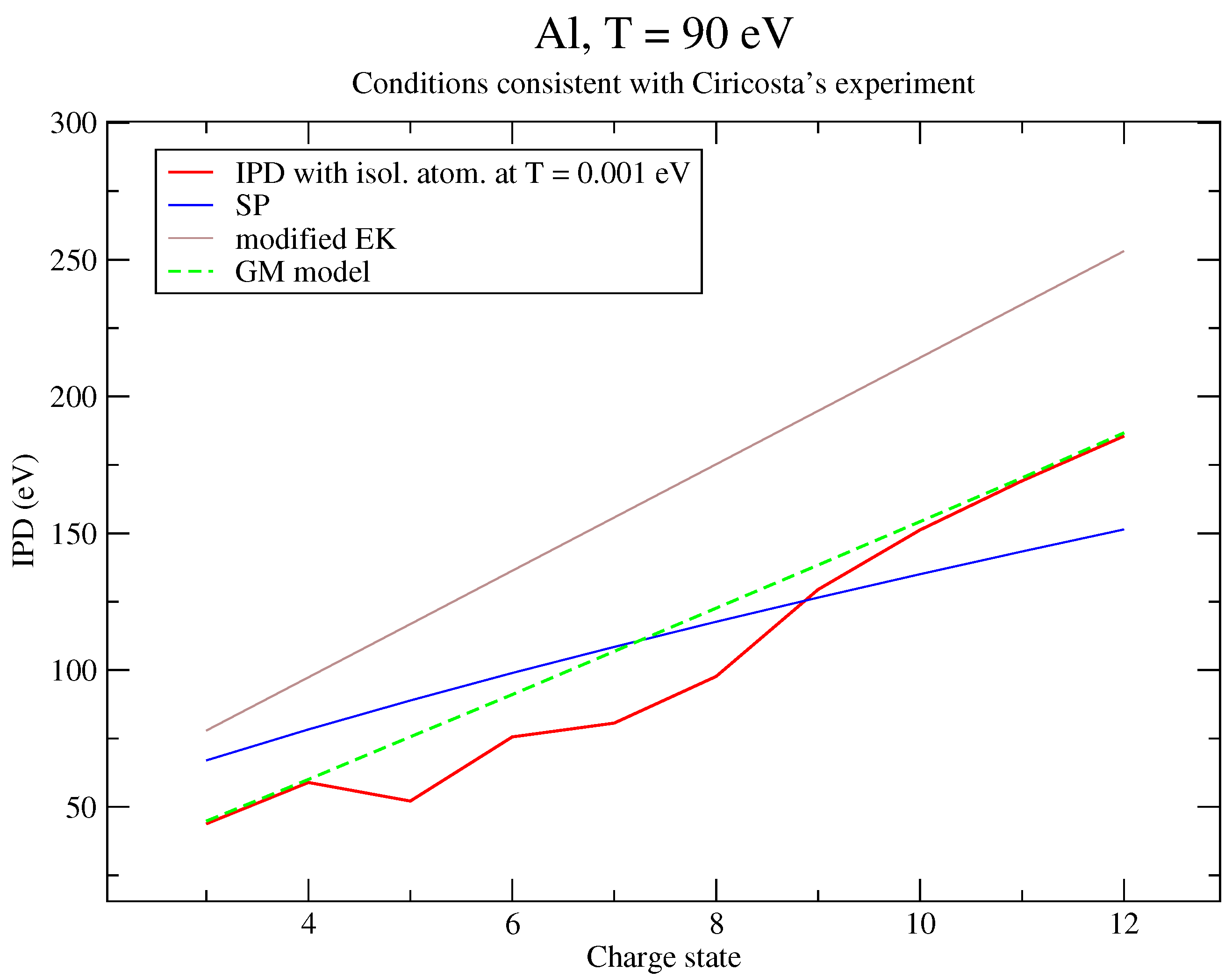
6. Discussion of the Results and Comparison to an Alternative Approach

6.1. Analysis of the Results

As mentioned in the introduction, ten years ago, Ciricosta et al. [30] used the Linac Coherent Light Source to generate solid-density aluminum plasmas at temperatures up to 180 eV. By varying the photon energy of the X rays that create and probe the plasma, they observed the K-fluorescence and could directly measure the position of the K edge of the ions in the plasma. The values they found disagree with the predictions of the SP model, but are consistent with the (modified) EK model, which predicts significantly larger depression of the ionization potential.

The Orion laser was used by Hoarty et al. [32] to study dense plasmas created by a combination of short pulse laser heating and compression by laser driven shocks. In that way, the plasma density was systematically varied between 1 and 10 g/cm³ using aluminum samples buried in plastic foils or diamond sheets. The aluminum plasma was heated to electron temperatures between 500 and 700 eV allowing the plasma conditions to be diagnosed by K-shell emission spectroscopy. The K-shell spectra show the effect of the ionization potential depression as a function of density. The measured data were compared to simulated spectra accounting for the change in the ionization potential by the SP and EK simple models and were found to be in closer agreement with simulations using the SP model.

The IPD is obtained by a simple procedure, consisting in subtracting the isolated-atom (infinite $R_{\mathrm{ws}}$ radius) subshell energy from the subshell energy subject to the plasma environment. In our modeling, the isolated-atom case is obtained using our electronic-structure code for a very large Wigner-Seitz radius (representing the limit where the electron density tends to zero). Figure 1, Figure 2, Figure 3, Figure 4 and Figure 5 display the IPD calculated using our approach and different analytical models (DH, SP, EK, modified EK) at temperatures consistent with Ciricosta’s experiment, i.e., T = 50, 70, 90, 120 and 180 eV.

The general trend is that our approach is always closer to SP for the lower charge states (keeping in mind that modified EK and SP are rather close in that case). For the highest charge states, at the lowest considered temperature (T = 50 eV), our results are closer to modified EK than SP, but the situation changes progressively as the temperature increases, and for the highest temperature (T = 180 eV) considered by Ciricosta [30], our results are closer to SP.

Figure 1, Figure 2, Figure 3, Figure 4 and Figure 5 also show the values obtained when the unscreened ionization potential, subtracted to the screened one subject to plasma effects, is taken at the plasma temperature. We can see that the quantity obtained that way (black dashed curve) increases with charge state. It is not an IPD stricto sensu, i.e., as commonly understood in the past and current works on the subject. Indeed, at plasma temperature T, excited states of a given ion are populated, and the ion “feels” the plasma environment differently as compared to the zero-temperature case (which corresponds to the “true” isolated atom). This has automatically an impact on the ionization potential.

Figure 6 represents the IPD of the different charge states for an aluminum plasma with different models in conditions related to Hoarty’s experiment with different modeling options. The figure shows a comparison between our work (with exchange-correlation and subtracted isolated-atom contribution taken at T = 0.001 eV), the values obtained by subtracting unscreened-atom ionization potential taken at the plasma temperature with exchange-correlation, the values obtained by subtracting unscreened-atom contribution taken at the plasma temperature without exchange-correlation, and usual analytical expressions: DH, SP, EK and modified EK.

This shows that accounting for exchange-correlation is important and that our results with T = 0.001 K isolated atom lie between EK and SP, while our results with the isolated atom taken at the real temperature are between SP and modified EK. Our results with unscreened ionization potential at T and no exchange-correlation are very close to modified EK, which is probably fortuitous (or at least difficult to interpret).

6.2. Reformulation of the Potential

The model presented in this subsection was presented by Massacrier a few years ago [46,47,48]; we will refer to it as “GM model” in the following. Let us consider the Poisson equation

$$V(r)=\frac{1}{r}{\int }_0^{r}4\pi r^{\prime 2}n(r^{\prime })d{r}^{\prime }+{\int }_r^{\infty }4\pi r^{\prime }n(r^{\prime })d{r}^{\prime }+D,$$

where

$$V(r)=\frac{Q(r)}{r}+{\int }_r^{\infty }\frac{1}{r^{\prime }}\frac{dQ}{dr}(r^{\prime })d{r}^{\prime }+D.$$

Massacrier suggested to use [46,47,48]:

$$V(r)=\frac{Q(r)}{r}-{\int }_0^r\frac{1}{r^{\prime }}\frac{dQ}{dr}(r^{\prime })d{r}^{\prime }+C,$$

(17)

where

$$C=D+{\int }_0^{\infty }\frac{1}{r^{\prime }}\frac{dQ}{dr}(r^{\prime })d{r}^{\prime }=D+{\int }_0^{\infty }4\pi r^{\prime }n(r^{\prime })d{r}^{\prime }$$

provided that the latter integral exists. Integrating Equation (17) by parts, one gets

$$V(r)=\frac{Q(r)}{r}-\left\{{\left[\frac{Q}{r^{\prime }}\right]}_0^r+{\int }_0^r\frac{Q(r^{\prime })}{r^{\prime 2}}d{r}^{\prime }\right\}+C=-{\int }_0^r\frac{Q(r^{\prime })}{r^{\prime 2}}d{r}^{\prime }+C+\frac{dQ}{dr}(0)$$

i.e.,

$$V(r)=-{\int }_0^r\frac{Q(r^{\prime })}{r^{\prime 2}}d{r}^{\prime }+V(0)$$

with

$$V(0)=C+\frac{dQ}{dr}(0).$$

If we apply this to the potential created by the free electrons, and with the notations used throughout the paper

$${\tilde{V}}_f(r)={\tilde{V}}_f(0)-{\tilde{E}}_f(r)$$

with

$${\tilde{Q}}_f(r)={\int }_0^{r}4\pi r^{\prime 2}{\tilde{n}}_f(r^{\prime })d{r}^{\prime }$$

and

$${\tilde{E}}_f(r)={\int }_0^r\frac{{\tilde{Q}}_f(r^{\prime })}{r^{\prime 2}}d{r}^{\prime }.$$

Taking Equation (16) for the expression of the IPD and neglecting the variations of the exchange-correlation potential and the influence of the free electron on the bound-electron density, one gets

$$\Delta V_k=\langle {\psi }_k|{\tilde{V}}_f|{\psi }_k\rangle +\frac{Z^{*}}{R_{\infty }},$$

i.e.,

$$\Delta V_k={\tilde{V}}_f(0)-\langle {\psi }_k|{\tilde{E}}_f|{\psi }_k\rangle +\frac{Z^{*}}{R_{\infty }}.$$

6.3. Correction to Recover Perturbation Theory

Setting

$$V_c(r)=-\frac{Z}{r}+V_b(r),$$

if $(V_c+{\tilde{V}}_f)\left(R_{\mathrm{ws}}\right)=0$, then

$$V_f(0)=\frac{z+1}{R_{\mathrm{ws}}}+{\int }_0^{\infty }\frac{{\tilde{Q}}_f(r)}{r^2}dr,$$

which is precisely the expression of the IPD used by Massacrier. However, perturbation theory teaches us that the IPD is equal, at first order, to

$$\langle {\psi }_k|{\tilde{V}}_f+\delta V_b+\delta V_{\mathrm{xc}}|{\psi }_k\rangle +V_{\mathrm{xc}}\left(R_{\mathrm{ws}}\right)-V_{\mathrm{xc}}\left(R_{\infty }\right)+\frac{Z^{*}}{R_{\infty }}.$$

Neglecting the variation of exchange-correlation and the influence of the free electrons on the bound-electron density ($\delta B_b=0$), one gets

$$\langle {\psi }_k|{\tilde{V}}_f|{\psi }_k\rangle +\frac{Z^{*}}{R_{\infty }}={\tilde{V}}_f(0)-\langle {\psi }_k|{\tilde{E}}_f|{\psi }_k\rangle +\frac{Z^{*}}{R_{\infty }}.$$

and taking $Z^{*}/R_{\infty }$, we find that the IPD should be stricto sensu

$$\mathrm{IPD}\left[\mathrm{GM}\mathrm{model}\right]={\tilde{V}}_f(0)-\langle {\psi }_k|{\tilde{E}}_f|{\psi }_k\rangle ,$$

meaning that the GM approach does not take into account the term

$$\langle {\psi }_k|{\tilde{E}}_f|{\psi }_k\rangle .$$

(18)

As can be checked in

Table 1. Correction to the IPD due to Equation (18) for an Al plasma at T = 70 eV and $\rho$ = 2.7 g/cm³ (conditions of Ciricosta’s experiment [30]).

${\mathit{Z}}^{\mathbf{*}}$	IPD (eV)	IPD + Corr. (eV)
3	45.4514	45.2086
4	61.1704	60.8535
5	76.731	76.338
6	92.6603	92.1946
7	108.447	107.908
8	124.383	123.772
9	140.522	139.841
10	156.718	155.968
11	173.024	172.208
12	189.777	188.912

,

Table 2. Correction to the IPD due to Equation (18) for an Al plasma at T = 180 eV and $\rho$ = 2.7 g/cm³ (conditions of Ciricosta’s experiment [30]).

${\mathit{Z}}^{\mathbf{*}}$	IPD (eV)	IPD + Corr. (eV)
3	43.3625	43.2009
4	58.0276	57.8132
5	73.0231	72.7569
6	88.1355	87.8175
7	103.047	102.678
8	118.151	117.730
9	133.214	132.742
10	148.368	147.846
11	163.623	163.052
12	179.232	178.624

and

Table 3. Correction to the IPD due to Equation (18) for an Al plasma (conditions of Hoarty’s experiment [32]).

${\mathit{Z}}^{\mathbf{*}}$	T (eV)	$\mathit{\rho }$ (g/cm3)	IPD (eV)	IPD + Corr. (eV)
12.3698	550	1.2	133.661	133.484
12.4739	650	2.5	172.536	172.194
12.3827	700	4	200.787	200.264
11.6673	550	5.5	212.477	211.729
12.0979	700	9	259.155	258.022
12.0762	700	11.6	282.298	280.847

, the contribution of such a term is small compared to ${\tilde{V}}_f(0)$) [46,47,48].

The values predicted by the GM model are close to ours and always higher. They coincide exactly with our values for the lowest and highest charge states and exhibit a linear behaviour (see Figure 7, Figure 8, Figure 9, Figure 10 and Figure 11). Figure 12 displays the IPD of the different charge states for an aluminum plasma with different models in conditions related to Ciricosta’s experiment (extreme temperatures 50 and 180 eV) compared to our the experimental values. It confirms that our results are close to the ones obtained by Massacrier (GM model), but always significantly smaller than the experimental values, whereas the latter lie between SP and EK (closer to SP for low charge sates, and to EK for high charge states).

7. Conclusions

We have presented a multi-configuration computation of the ionization potential depression in the framework of density functional theory. The IPD is obtained by a simple procedure, consisting in subtracting the isolated-atom (infinite $R_{\mathrm{ws}}$ radius) subshell energy from the subshell energy in the presence of the plasma environment. Several theoretical aspects were considered, such as the connection with perturbation theory, and the relative importance of the different contributions. In our case, the isolated atom is obtained using our electronic-structure code for a very large Wigner-Seitz radius (representing the case where the electron density tends to zero). It turns out that the temperature at which the unscreened-atom ionization potential is computed changes drastically the results; the values are different, as well as the variations.

Following the usual definition, in order to compare with analytical modified EK and SP models, the true IPD requires the evaluation of the unscreened ionization potential at the lowest temperature as possible (in the present work T = 0.001 eV, the lowest temperature which could be computed with our code), which corresponds to the isolated-atom value. The IPD, calculated in that way, decreases with charge state. We discussed also the values obtained when the unscreened ionization potential, subtracted to the screened one subject to plasma effects, is taken at the plasma temperature. The quantity obtained that way (which is not a real IPD) increases with charge state.

The general trend is that our approach is always closer to SP for the lowest charge states (keeping in mind that modified EK and SP are rather close in that case). As concerns the higher charge states, at the lowest considered temperature (T = 50 eV), our results are closer to modified EK than SP, but the situation changes progressively as the temperature increases, and for the highest considered temperature (T = 180 eV), our results are in better agreement with SP.

Concerning the Hoarty experiment, our results with T = 0.001 K isolated atom lie between EK and SP, while the values obtained with the unscreened ionization potential taken at the real temperature are between SP and modified EK. The values obtained while taking the unscreened ionization potential at the plasma temperature T and no exchange-correlation are very close to modified EK.

As concerns the Ciricosta experiment, our results are close to the one obtained by Massacrier (GM model), but always significantly smaller than the experimental values, whereas the latter lie between SP and EK (closer to SP for low charge sates, and to EK for high charge states).

References

1. Brillet, W.-Ü.L.; Artru, M.-C. Extension of the Analysis of Quadruply Ionized Silicon (Si V). Phys. Scr. 1976, 14, 285–289. [Google Scholar] [CrossRef]
2. Obadasi, H. Regularities in ionization potentials. Phys. Scr. 1979, 19, 313–317. [Google Scholar]
3. Liu, P.; Gao, C.; Hou, Y.; Zeng, J.; Yuan, J. Transient space localization of electrons ejected from continuum atomic processes in hot dense plasma. Commun. Phys. 2018, 1, 95–101. [Google Scholar] [CrossRef]
4. Lin, C. Ionization Potential Depression and Ionization Balance in Dense Plasmas. arXiv 2019, arxiv:1904.04456. [Google Scholar]
5. Lin, C. Quantum statistical approach for ionization potential depression in multi-component dense plasmas. Phys. Plasmas 2019, 26, 122707. [Google Scholar] [CrossRef]
6. Zeng, J.; Li, Y.; Hou, Y.; Gao, C.; Yuan, J. Ionization potential depression and ionization balance in dense carbon plasma under solar and stellar interior conditions. A&A 2020, 644, A92. [Google Scholar]
7. Pain, J.-C. A model of dense-plasma atomic structure for equation-of-state calculations. J. Phys. B At. Mol. Opt. Phys. 2007, 40, 1553–1573. [Google Scholar] [CrossRef]
8. Pain, J.-C.; Dejonghe, G. Electrical Resistivity in Warm Dense Plasmas Beyond the Average-Atom Model. Contrib. Plasma Phys. 2010, 50, 39–45. [Google Scholar] [CrossRef]
9. Wetta, N.; Pain, J.-C. Consistent approach for electrical resistivity within Ziman’s theory from solid state to hot dense plasma: Application to aluminum. Phys. Rev. E 2020, 102, 053209. [Google Scholar] [CrossRef]
10. Wetta, N.; Pain, J.-C. Issues in the calculation of dc conductivity of warm dense aluminum. Contrib. Plasma Phys. 2022, e202200003. [Google Scholar] [CrossRef]
11. Pain, J.-C.; Dejonghe, G.; Blenski, T. Quantum-mechanical model for the study of pressure ionization in the superconfiguration approach. J. Phys. A Math. Gen. 2006, 39, 4659–4666. [Google Scholar] [CrossRef]
12. Pain, J.-C.; Dejonghe, G.; Blenski, T. A self-consistent model for the study of electronic properties of hot dense plasmas. J. Quant. Spectrosc. Radiat. Transf. 2006, 99, 451–468. [Google Scholar] [CrossRef]
13. Rogers, F.J.; Iglesias, C.A. Astrophysical opacity. Science 1994, 263, 50–55. [Google Scholar] [CrossRef] [PubMed]
14. Guillot, T. Interiors of giant planets inside and outside the solar system. Science 1999, 286, 72–77. [Google Scholar] [CrossRef] [PubMed]
15. Potekhin, A.Y.; Massacrier, G.; Chabrier, G. Equation of state for partially ionized carbon at high temperatures. Phys. Rev. E 2005, 72, 046402. [Google Scholar] [CrossRef] [PubMed]
16. Massacrier, G.; Potekhin, A.Y.; Chabrier, G. Equation of state for partially ionized carbon and oxygen mixtures at high temperatures. Phys. Rev. E 2011, 84, 056406. [Google Scholar] [CrossRef] [PubMed]
17. Lindl, J.D.; Amendt, P.; Berger, R.L.; Glendinning, S.G.; Glenzer, S.H.; Haan, S.W.; Kauffman, R.L.; Landen, O.L.; Suter, L.J. The physics basis for ignition using indirect-drive targets on the National Ignition Facility. Phys. Plasmas 2004, 11, 339–491. [Google Scholar] [CrossRef]
18. Hu, S.X.; Militzer, B.; Goncharov, V.N.; Skupsky, S. Strong Coupling and Degeneracy Effects in Inertial Confinement Fusion Implosions. Phys. Rev. Lett. 2010, 104, 235003. [Google Scholar] [CrossRef]
19. Jarrah, W.; Pain, J.-C.; Benredjem, D. Plasma potential and opacity calculations. High Energy Density Phys. 2019, 32, 8–13. [Google Scholar] [CrossRef]
20. Pain, J.-C.; Benredjem, D. Simple electron-impact excitation cross-sections including plasma density effects. High Energy Density Phys. 2021, 38, 100923. [Google Scholar] [CrossRef]
21. Bruce, R.E.; Todd, F.C. Lowering of the Ionization Potential in Dense Aluminum Plasmas. Proc. Okla. Acad. Sci. 1963, 95–102. [Google Scholar]
22. Zaghloul, M.R. Thermodynamic depression of ionization potentials in nonideal plasmas: Generalized self-consistency criterion and a backward scheme for deriving the excess free energy. Astrophys. J. 2009, 699, 885–891. [Google Scholar] [CrossRef]
23. Crowley, B.J.B. Continuum lowering, a new perspective. High Energy Density Phys. 2014, 13, 84–102. [Google Scholar] [CrossRef]
24. Massacrier, G.; Böhme, M.; Vorberger, J.; Soubiran, F.; Militzer, B. Reconciling ionization energies and band gaps of warm dense matter derived with ab initio simulations and average atom models. Phys. Rev. Res. 2021, 3, 023026. [Google Scholar] [CrossRef]
25. Zan, X.; Lin, C.; Hou, Y.; Yuan, J. Local field correction to ionization potential depression of ions in warm or hot dense matter. Phys. Rev. E 2021, 104, 025203. [Google Scholar] [CrossRef]
26. Callow, T.J.; Hansen, S.B.; Kraisler, E.; Cangi, A. First-principles derivation and properties of density-functional average-atom models. Phys. Rev. Res. 2022, 4, 023055. [Google Scholar] [CrossRef]
27. Ecker, G.; Kröll, W. Lowering of the Ionization Energy for a Plasma in Thermodynamic Equilibrium. Phys. Fluids 1963, 6, 62–69. [Google Scholar] [CrossRef]
28. Stewart, J.C.; Pyatt, K.D., Jr. Lowering of ionization potentials in plasmas. Astrophys. J. 1966, 144, 1203–1211. [Google Scholar] [CrossRef]
29. LCLS. Available online: http://lcls.slac.stanford.edu/ (accessed on 14 September 2022).
30. Ciricosta, O.; Vinko, S.M.; Chung, H.-K.; Cho, B.-I.; Brown, C.R.D.; Burian, T.; Chapulsky, J.; Engelhorn, K.; Falcone, R.W.; Graves, C.; et al. Direct Measurements of the Ionization Potential Depression in a Dense Plasmas. Phys. Rev. Lett. 2012, 109, 065002. [Google Scholar] [CrossRef]
31. Ciricosta, O.; Vinko, S.M.; Barbrel, B.; Rackstraw, D.S.; Preston, T.R.; Burian, T.; Chalupský, J.; Cho, B.I.; Chung, H.-K.; Dakovski, G.L.; et al. Measurements of continuum lowering in solid-density plasmas created from elements and compounds. Nat. Commun. 2016, 7, 11713. [Google Scholar] [CrossRef]
32. Hoarty, D.J.; Allan, P.; James, S.F.; Brown, C.R.D.; Hobbs, L.M.R.; Hill, M.P.; Harris, J.W.O.; Morton, J.; Brookes, M.G.; Shepherd, R.; et al. Observations of the Effect of Ionization-Potential Depression in Hot Dense Plasma. Phys. Rev. Lett. 2013, 110, 265003. [Google Scholar] [CrossRef]
33. Fletcher, L.B.; Kritcher, A.L.; Pak, A.; Ma, T.; Döppner, T.; Fortmann, C.; Divol, L.; Jones, O.S.; Landen, O.L.; Scott, H.A.; et al. Observations of Continuum Depression in Warm Dense Matter with X-Ray Thomson Scattering. Phys. Rev. Lett. 2014, 112, 145004. [Google Scholar] [CrossRef] [PubMed]
34. Kraus, D.; Chapman, D.A.; Kritcher, A.L.; Baggott, R.A.; Bachmann, B.; Collins, G.W.; Glenzer, S.H.; Hawreliak, J.A.; Kalantar, D.H.; Landen, O.L.; et al. X-ray scattering measurements on imploding CH spheres at the National Ignition Facility. Phys. Rev. E 2016, 94, 011202. [Google Scholar] [CrossRef] [PubMed]
35. Son, S.-K.; Thiele, R.; Jurek, Z.; Ziaja, B.; Santra, R. Quantum-mechanical calculation of ionization potential lowering in dense plasmas. Phys. Rev. X 2014, 4, 031004. [Google Scholar] [CrossRef] [Green Version]
36. Vinko, S.M.; Ciricosta, O.; Wark, J.S. Density functional theory calculations of continuum lowering in strongly coupled plasmas. Nat. Commun. 2014, 5, 3533. [Google Scholar] [CrossRef]
37. Hu, S.X. Continuum Lowering and Fermi-Surface Rising in Strongly Coupled and Degenerate Plasmas. Phys. Rev. Lett. 2017, 119, 065001. [Google Scholar] [CrossRef]
38. Calisti, A.; Ferri, S.; Talin, B. Ionization Potential Depression in Hot Dense Plasmas Through a Pure Classical Model. Contrib. Plasma Phys. 2015, 55, 360–365. [Google Scholar] [CrossRef]
39. Stransky, M. Monte Carlo simulations of ionization potential depression in dense plasmas. Phys. Plasmas 2016, 23, 012708. [Google Scholar] [CrossRef]
40. Iglesias, C.A.; Sterne, P.A. Fluctuations and the ionization potential in dense plasmas. High Energy Density Phys. 2013, 9, 103–107. [Google Scholar] [CrossRef]
41. Lin, C.; Kraeft, W.-D.; Röpke, G.; Reinholz, H. Ionization-potential depression and dynamical structure factor in dense plasmas. Phys. Rev. E 2017, 96, 013202. [Google Scholar] [CrossRef]
42. Rosmej, F.B. Ionization potential depression in an atomic-solid-plasma picture. J. Phys. B At. Mol. Opt. Phys. 2018, 51, 09LT01. [Google Scholar] [CrossRef]
43. Alexiou, S.; Stambulchik, E.; Gomez, T.; Koubiti, M. The Fourth Workshop on Lineshape Code Comparison: Line merging. Atoms 2018, 6, 13. [Google Scholar] [CrossRef]
44. Stein, J. Line shifts in plasmas: A quantum mechanical approach. J. Quant. Spectrosc. Radiat. Transf. 1995, 54, 395–399. [Google Scholar] [CrossRef]
45. Ren, S.; Shi, Y.; van den Berg, Q.Y.; Firmansyah, M.; Chung, H.-K.; Fernandez-Tello, E.V.; Velarde, P.; Wark, J.S.; Vinko, S.M. Non-thermal evolution of dense plasmas driven by intense X-ray fields. arXiv 2022, arXiv:2208.00573v3. [Google Scholar]
46. Massacrier, G. Self-consistent schemes for the calculation of ionic structures and populations in dense plasmas. J. Quant. Spectrosc. Radiat. Transf. 1994, 51, 221–228. [Google Scholar] [CrossRef]
47. Massacrier, G. Ionization potential depression in warm and hot solid-density plasma. In Proceedings of the HEDLA (High Energy Density Laboratory Astrophysics), Bordeaux, France, 12–16 May 2014. [Google Scholar]
48. Massacrier, G. Ionization potential depression in warm dense matter conditions. In Proceedings of the ILP (Fédération Lasers et Plasmas) Forum, Porquerolles, France, 14–19 June 2015. [Google Scholar]
49. Debye, P.; Hückel, E. On the theory of electrolytes, I. Freezing point depression and related phenomena. Phys. Z 1923, 24, 185–206. [Google Scholar]
50. Preston, T.R.; Vinko, S.M.; Ciricosta, O.; Chung, H.-K.; Lee, R.W.; Wark, J.S. The effects of ionization potential depression on the spectra emitted by hot dense aluminum plasmas. High Energy Density Phys. 2013, 9, 258–263. [Google Scholar] [CrossRef]
51. Pain, J.-C. Super Transition Arrays: A Tool for Studying Spectral Properties of Hot Plasmas. Plasma 2021, 4, 42–64. [Google Scholar] [CrossRef]
52. Pain, J.-C. Adaptive Algorithm for the Generation of Superconfigurations in Hot-Plasma Opacity Calculations. Plasma 2022, 5, 154–175. [Google Scholar] [CrossRef]
53. More, R.M. Pressure Ionization, Resonances, and the Continuity of Bound and Free States. Adv. At. Mol. Phys. 1985, 21, 305–356. [Google Scholar]
54. Blenski, T.; Ishikawa, K. Pressure ionization in the spherical ion-cell model of dense plasmas and a pressure formula in the relativistic Pauli approximation. Phys. Rev. E 1995, 51, 4869–4881. [Google Scholar] [CrossRef] [PubMed]
55. Froese-Fischer, C. The Hartree-Fock Method for Atoms: A Numerical Approach; John Wiley & Sons: New York, NY, USA, 1977. [Google Scholar]
56. Benredjem, D.; Pain, J.-C.; Calisti, A.; Ferri, S. Ionization by electron impacts and ionization potential depression. J. Phys. B At. Mol. Opt. Phys. 2022, 55, 105001. [Google Scholar] [CrossRef]
57. Hartree, D.R. The Calculation of Atomic Structures; John Wiley: New York, NY, USA, 1957. [Google Scholar]
58. Nikiforov, A.F.; Novikov, V.G.; Uvarov, V.B. Quantum Statistical Models of Hot Dense Matter; Birkhauser: Basel, Switzerland, 2005. [Google Scholar]
59. Pain, J.-C. Résolution de l’équation de Schrödinger à une Dimension par la Méthode de la Fonction Phase. Master’s Thesis, CEA & Ecole Normale Supérieure, Paris, France, 1999. (In French). [Google Scholar]
Figure 1. IPD of the different charge states for an aluminum plasma at T = 50 eV: our calculation (present work) with the isolated atom at T = 0.001 eV (red curve), Debye-Hückel model (green curve), Ecker-Kröll model (magenta dashed curve) and modified Ecker-Kröll model (brown curve). The dashed black curve represents the modification of the ionization potential when the isolated atom value is taken at the plasma temperature (T = 50 eV). It does not correspond to the definition underlying the other approaches and is not an IPD stricto sensu.
Plasma 05 00029 g001
Figure 2. Same as Figure 1 but with a plasma temperature of T = 70 eV.
Plasma 05 00029 g002
Figure 3. Same as Figure 1 but with a plasma temperature of T = 90 eV.
Plasma 05 00029 g003
Figure 4. Same as Figure 1 but with a plasma temperature of T = 120 eV.
Plasma 05 00029 g004
Figure 5. Same as Figure 1 but with a plasma temperature of T = 180 eV.
Plasma 05 00029 g005
Figure 6. IPD of the different charge states for an aluminum plasma with different models in conditions related to Hoarty’s experiment with different modeling options. Black: this work with exchange-correlation and subtracted unscreened atom contribution taken at the expected plasma temperature, red: the same but with subtracted isolated-atom contribution taken at T = 0.001 eV, green: this work without exchange-correlation and subtracted unscreened atom contribution taken at the expected plasma temperature, dashed blue: Debye-Hückel, magenta: Stewart-Pyatt, brown: Ecker-Kröll and purple: modified Ecker-Kröll.
Plasma 05 00029 g006
Figure 7. IPD of the different charge states for an aluminum plasma at T = 50 eV: our calculation (red curve), Stewart-Pyatt model (blue curve), modified Ecker-Kröll model (brown curve) and GM model (green dashed curve).
Plasma 05 00029 g007
Figure 8. IPD of the different charge states for an aluminum plasma at T = 70 eV: our calculation (red curve), Stewart-Pyatt model (blue curve), modified Ecker-Kröll model (brown curve) and GM model (green dashed curve).
Plasma 05 00029 g008
Figure 9. IPD of the different charge states for an aluminum plasma at T = 90 eV: our calculation (red curve), Stewart-Pyatt model (blue curve), modified Ecker-Kröll model (brown curve) and GM model (green dashed curve).
Plasma 05 00029 g009
Figure 10. IPD of the different charge states for an aluminum plasma at T = 120 eV: our calculation (red curve), Stewart-Pyatt model (blue curve), modified Ecker-Kröll model (brown curve) and GM model (green dashed curve).
Plasma 05 00029 g010
Figure 11. IPD of the different charge states for an aluminum plasma at T = 180 eV: our calculation (red curve), Stewart-Pyatt model (blue curve), modified Ecker-Kröll model (brown curve) and GM model (green dashed curve).
Plasma 05 00029 g011
Figure 12. IPD of the different charge states for an aluminum plasma in conditions compatible with Ciricosta’s experiment [30] with different models (red: SP, blue: experimental values, brown: modified EK, brown, cyan: GM model, purple: this work). Histograms: full = lowest temperature T = 50 eV, empty (or zebra): highest temperature T = 180 eV.
Plasma 05 00029 g012