Simulation of the First Two Microseconds of an Ar CCP Cold Plasma Discharge by the PIC-MCC Method

Abstract

Most simulations of capacitively coupled radiofrequency cold-plasma discharges (RF-CCP) are focused on the steady state, but the initial discharge time is important for understanding the ignition process and the behavior of pulsed discharges. In this work, the time evolution of an RF-CCP Ar discharge was simulated, considering a pressure of 66.6 Pa, a distance between the electrodes of 20 mm, and RF (13.56 MHz) bias amplitudes in range 100–400 V, and the discharge evolution was observed for the first 2 μs. A 1d3v (1 dimension for particle positions and 3 dimensions for particle velocities) electrostatic particle in cell with montecarlo collisions (PIC-MCC) model was used, with separated particle weights for electrons and ions that varied with the particle density. During the simulations, the time evolution of the electron density, mean electron energy, Debye length, Debye number, and plasma frequency were observed. The spatial distribution of electric potential and the electron energy distribution function were also monitored. A transition between two regimes was observed; the first was characterized by strong oscillation of the mean electron energy and an exponential increase of the mean plasma density with time, while in the second the mean electron energy was lower, and the plasma density increased linearly. The time required for the transition between the two regimes increased as the RF amplitude was raised from 100 to 250 V, then decreased with a further increase of the RF amplitude to 300 and 350 V.

1. Introduction

Capacitively coupled cold-plasma discharges activated by radiofrequency (RF-CCP) [1] are of widespread use for thin-film deposition and surface modification processes [2] in a wide range of applications, including microelectronics [3], photovoltaics [4], energy-saving materials [5], pollution control [6], as well as biological applications [7,8,9]. Among RF-CCP discharges, those working at low pressure (lower than atmospheric) have been in use for a longer time, despite their requirement for expensive vacuum systems, because they require less power to be activated compared with atmospheric pressure discharges, and are less sensitive to contamination by atmospheric gases. [1].

Due to their importance, considerable experimental and theoretical work has been carried out to improve the understanding of the physico-chemical processes involved in low-pressure RF-CCP discharges. However, most of the experimental and simulation work has focused on the characteristics of the steady state when the plasma parameters have reached a stationary condition, as this is the regime in which the technological applications of the plasma discharge, such as thin-film deposition or surface etching, are more controllable. However, the initial part of the process, which is required for the onset of a stable discharge, is important for understanding the plasma ignition, as well as for the study of pulsed discharges. In fact, several experimental and theoretical works have been published in recent years to describe some aspects of the evolution with time of plasma parameters in different types of capacitively coupled RF discharges. These studies have particularly focused on pulsed discharges, and most of them have dealt with a time scale using microsecond [10,11,12], millisecond [13], or even second [14] resolution, while less information can be found relating to time evolution with nanosecond resolution [15,16]. However, according to the results obtained in this work, transition between different discharge mechanisms can take place at the very beginning of the discharge, in a time lower than one microsecond.

In this work, a low-pressure capacitively coupled discharge in a parallel-plate reactor was simulated, starting from the first activation of the electric bias on the electrodes and tracking the discharge evolution through time for 2 μs. A 1d3v electrostatic PIC-MCC model was used, with particle weights different for electrons and ions and which varied as the numbers of electrons and ions increased, allowing the number of superparticles to remain in a limited range, even with dramatic changes in the number of real particles. The time evolution of several quantities was followed during the simulation, including the mean electron energy, the electron density n_e, the Debye length λ_D, the Debye number N_D and the plasma frequency ν_P. The spatial distribution of the electric potential inside the discharge was also monitored, as well as the electron energy distribution function (EEDF).

2. Materials and Methods

2.1. Physical Characteristics of the Simulated Discharge

In this work, a parallel-plate, radio-frequency, low-pressure Ar discharge was simulated, using the physical parameters showed in

Table 1. Physical characteristics of the simulated discharge.

Quantity	Symbol	Value	Unit
Electrodes lateral length	l	250	mm
Distance between the electrodes	d	20	mm
Plasma volume	Vpla = l2 · d	1.25 × 10−3	m3
Gas temperature	Tgas	300	K
Gas pressure	p	66.6	Pa
Gas molecule density	ngas	1.6 × 1022	m−3
Electric bias peak value	∆Vmax	100	V
		150
		200
		250
		300
		350
		400
Electric bias frequency	νRF	13.56	MHz
Electric bias period	τRF = 1/νRF	73.75	ns
Electric bias starting phase	φ0	0	°

. The gas temperature T_gas and pressure p were fixed at 300 K and 66.6 Pa (0.5 Torr), respectively, and the distance d between the two planar electrodes set to 20 mm, providing a pd value of 1.33 Pa m (1 Torr cm). The electrodes were of square shape and their lateral length was chosen to provide a sufficiently large plasma volume to obtain at least some hundreds of free electrons and ions inside the discharge at the beginning of the simulation. A radiofrequency sinusoidal signal with a frequency of 13.56 MHz was used to simulate the electric bias applied between the electrodes, and seven values of the signal amplitude were compared: 100, 150, 200, 250, 300, 350, and 400 V. The initial phase of the sinusoidal signal was fixed at 0 degrees, which means that at t = 0 s the potential difference between the electrodes was 0 V.

2.2. Details of the Simulation Process

The simulations were carried out using CCPLA software (version 0.2.0, Pietro Mandracci, Turin, Italy) which is freely available online. The software is designed to simulate a gas discharge in the volume comprised between two parallel square electrodes, between which a DC or RF signal is applied, and inside which a gas or gas mixture at low pressure is confined. The details of the CCPLA software are reported in Appendix A.

The main simulation parameters are reported in

Table 2. Simulation parameters.

Quantity	Symbol	Value	Unit
Starting ionization degree	α(0)	4 × 10−17
Starting electron density	ne(0) = ngas · α(0)	6.41 × 105	m−3
Simulation time step	∆t	10	ps
Time between data acquisitions	∆toutput	1	ns
Overall simulated time	∆ttotal	2	μs
Maximum number of computational particles	Nemax	5 × 104
Number of PIC cells (1D)	Nz	300
Dimension of a PIC cell	∆z	66.67	μm

. An initial ionization degree of 4 × 10⁻¹⁷ was considered, which is consistent with positive ion density at atmospheric pressure of about 10⁹ m⁻³, usually reported for air in a closed environment [17,18]. Considering the given Ar gas pressure of 66.6 Pa, this value provides an initial electron density of 6.4 × 10⁵ m⁻³, and an initial number of computational particles of about 800 for each particle type (electrons and Ar⁺ ions). The starting positions of the electrons and ions in the plasma volume were determined randomly, following uniform distributions along the x, y, and z axes. The particle speeds were randomly extracted according to the Maxwell–Boltzmann distribution, with a temperature equal to the one of the neutral Ar atoms (300 K), while the initial velocity directions were randomly determined with uniform distribution of the solid angle.

The number density of the neutral Ar atoms was considered constant throughout the simulation time, neglecting its variation due to the transformation of neutral atoms in ions provided by the ionization processes. This approximation is justified by the maximum electron density obtained during the simulation, which was always lower than 10¹⁵ m⁻³ (see Section 3.1), seven orders of magnitude lower than the neutral density n_gas ~ 10²² m⁻³.

A constant time step ∆t = 10 ps was chosen, and the space between the electrodes was divided into 300 one-dimensional cells of size ∆z = 66.7 μm. These values were chosen to satisfy the usual requirements for stability and accuracy of the PIC simulation scheme [19]:

• the RF period was divided in 7375 time steps, providing good resolution of the RF behavior;
• the probability of obtaining a collision during a time step (given by Equation (A1)) was lower than 0.05, providing a negligible probability of multiple collisions during a time step;
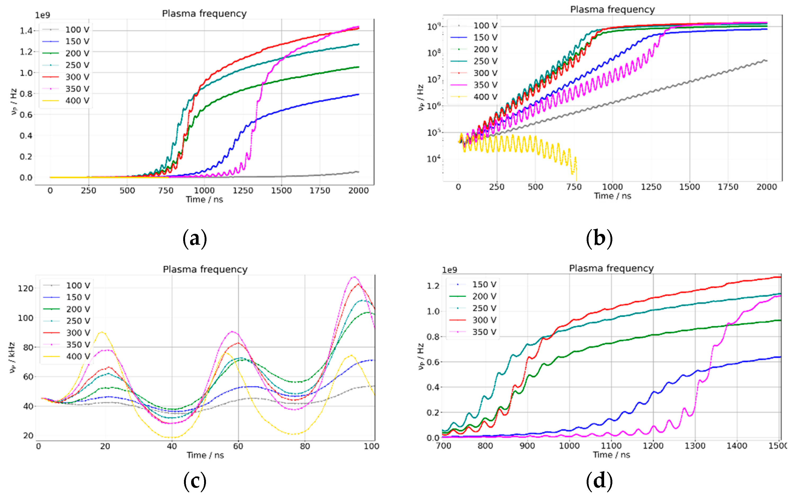
• considering that the plasma frequency was always ν_P < 2 × 10⁹ s⁻¹ during all simulation runs (see Section 3.5), the condition ν_P ∆t < 0.1 was always satisfied;
• considering that the minimum value of the Debye length was about 200 μm (see Section 3.3), the condition ∆z < λ_D was always satisfied;
• the particles were not able to travel a distance greater than ∆z during a time step; the speed required to do so is v = ∆z/∆t = 6.67 × 10⁶ m s⁻¹, which for an electron requires a kinetic energy of about 126 keV, much higher than the electron energy in the EEDF tails (see Section 3.7).

Certain boundary conditions were used by the Poisson solver for the electric potential calculation; the grounded electrode positioned at z = 20 mm was considered at a fixed potential of zero volts, while the potential at the biased electrode positioned at z = 0 mm was considered equal to the value of the RF amplitude at the given simulation time. The electrons and ions were removed from the discharge when they reached one of the electrodes (z equal to 0 or 20 mm), while if they reached one of the electrode borders (x or y equal to 0 or 250 mm) they were made to re-enter on the opposite side. The emission of secondary electrons from the electrodes was not included in the model.

The simulation model included elastic, excitation, and ionization collisions for electrons, and elastic and charge exchange collisions for ions, as shown in

Table 3. Collision processes considered in the simulation.

Collision Type	First Particle	Second Particle	Ref.
Elastic	Electron	Ar atom	[20]
Excitation	Electron	Ar atom	[20]
Ionization	Electron	Ar atom	[20]
Elastic	Ar+ ion	Ar atom	[21]
Charge exchange	Ar+ ion	Ar atom	[21]

. The Ar atoms were considered at rest for the electron–atom collisions, while for collisions between an ion and an atom both were considered moving and the collision was simulated inside the center of mass frame of reference (COMFOR). More details of the collision processes are given in Appendix A.

The simulations required between four and five hours to be completed, run on a PC equipped with an octacore CPU (AMD Ryzen 7 4800 H) using a single core only at a clock frequency of 4.2 GHz for the numerical computation cycles, while more cores were used to manage the software GUI and the runtime plots.

2.3. Calculated Plasma Parameters

The time evolution of various physical quantities was considered during the simulation runs, i.e.: electron density n_e, electron mean energy <E_e>, Debye length λ_D and number N_D, and plasma frequency ν_P. The electron density and the electron mean energy were simulated directly by the CCPLA software during the simulation runs, and the other three quantities were calculated as described in Appendix B. The spatial distribution of the electric potential along the direction normal to the electrodes (z axis) was also monitored, and selected samples are reported in Section 3.6. The electron energy distribution function (EEDF) was monitored, and samples acquired at different simulation times are reported in Section 3.7.

3. Results

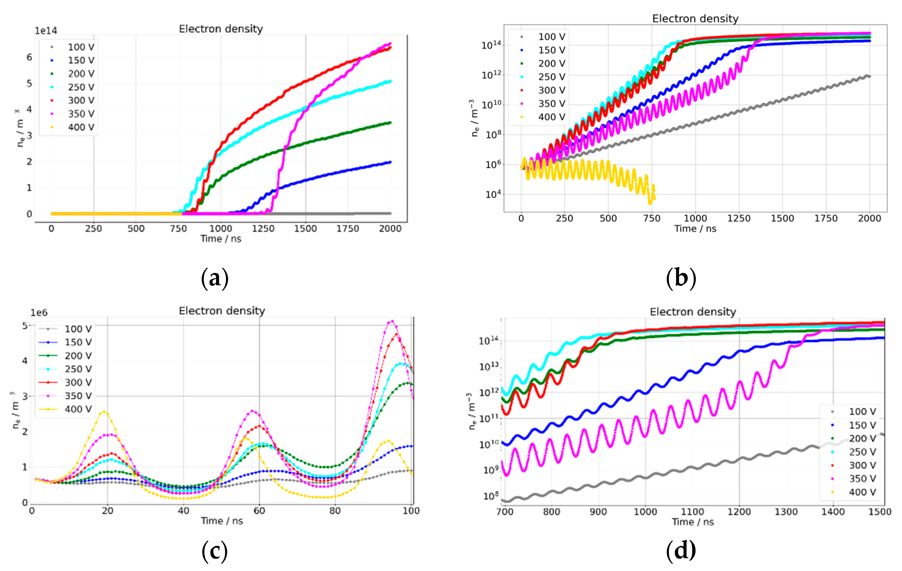
3.1. Electron Density

The time evolution of the electron density, for electric bias peak values between 100 and 400 V, is shown in Figure 1, using (a) linear and (b) semilogarthmic scales. Zoomed graphs of (c) the first 100 ns in linear scale and (d) the 700–1500 ns range in semilogarithmic scale are also provided. For bias voltage values in the 150–350 V range, a quite abrupt change between two different regimes was observed, first up to about 750–1250 ns, depending on the bias voltage, and a second after about 1–1.5 μs, with a transition region between the two regimes. For the 100 V peak bias value there was no transition, and the first regime was observed up to 2 μs of simulated time. For the 400 V peak bias, contrastingly, the mean value of electron density decreased with time, and after about 750 ns it dropped to zero, meaning that no more electrons were present in the simulated discharge.

In the first regime, for the 100–350 V peak bias voltages, the electron density was too low to be visible in the linear plot of Figure 1a, but the semilogarithmic plots of Figure 1b,d show an oscillating behavior, while the time average (ideal line in the middle between the maxima and minima) followed an approximately linear behavior in the semilogarthmic scale, thus evidencing an exponential increase with time. The slope of this mean value in the semilogarithmic plot increased for voltage values from 100 to 250 V, then decreased for the 300 and 350 V values, as seen in Figure 1b,d. Moreover, the semilogarithmic plot related to the 350 V peak bias shows a deviation from linearity at about 750 ns. The oscillation amplitude appeared constant with time in the semilogarithmic scale, which means that the ratio between the adjacent maxima and minima remained approximately constant. Figure 1c shows a zoom of the first 100 ns in linear scale, evidencing more clearly the oscillating behavior. An increase in amplitude with time was observed for all signals except for the 400 V peak bias voltage, for which a slow decrease of the electron density oscillation amplitude was observed with time.

In the second regime, after about 1 μs of simulated time for the 300 V peak bias voltage, a linear increase of the electron density with time is clearly visible in Figure 1a, appearing as an almost flat line in the semilogarithmic scales of Figure 1b,d. Moreover, the oscillation of electron density with time appears much less intense, compared with the first region. The time required for the transition between the two regimes reduced as the peak bias voltage increased from 150 to 250 V, then the transition time increased for 300 V and 350 V. For the 100 V value there was no transition up to the maximum simulated time, and for 400 V the simulation ended during the first regime. In the second regime, from 150 to 350 V the slope of the electron density linear increase rose with the peak bias voltage, as seen in Figure 1a.

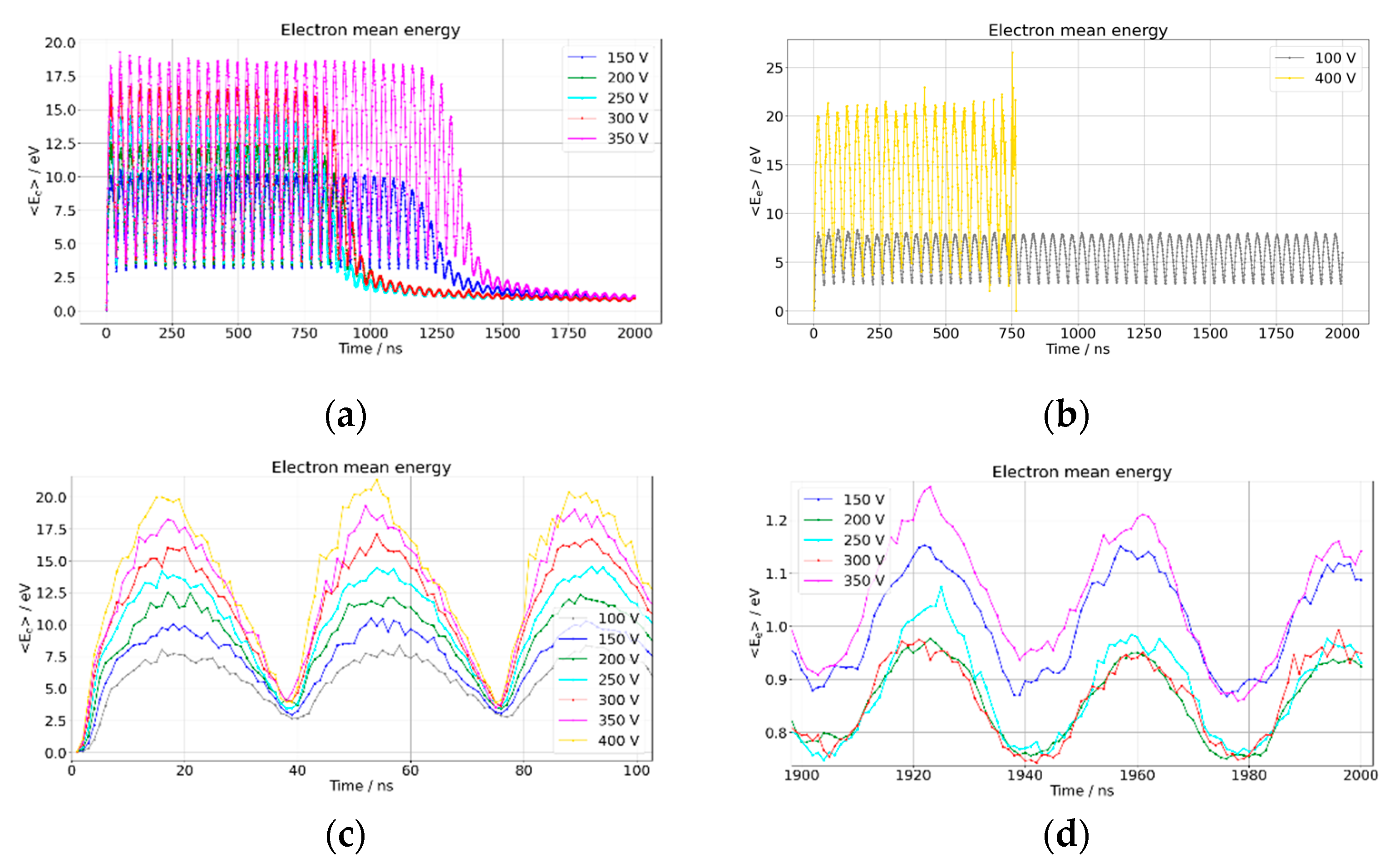
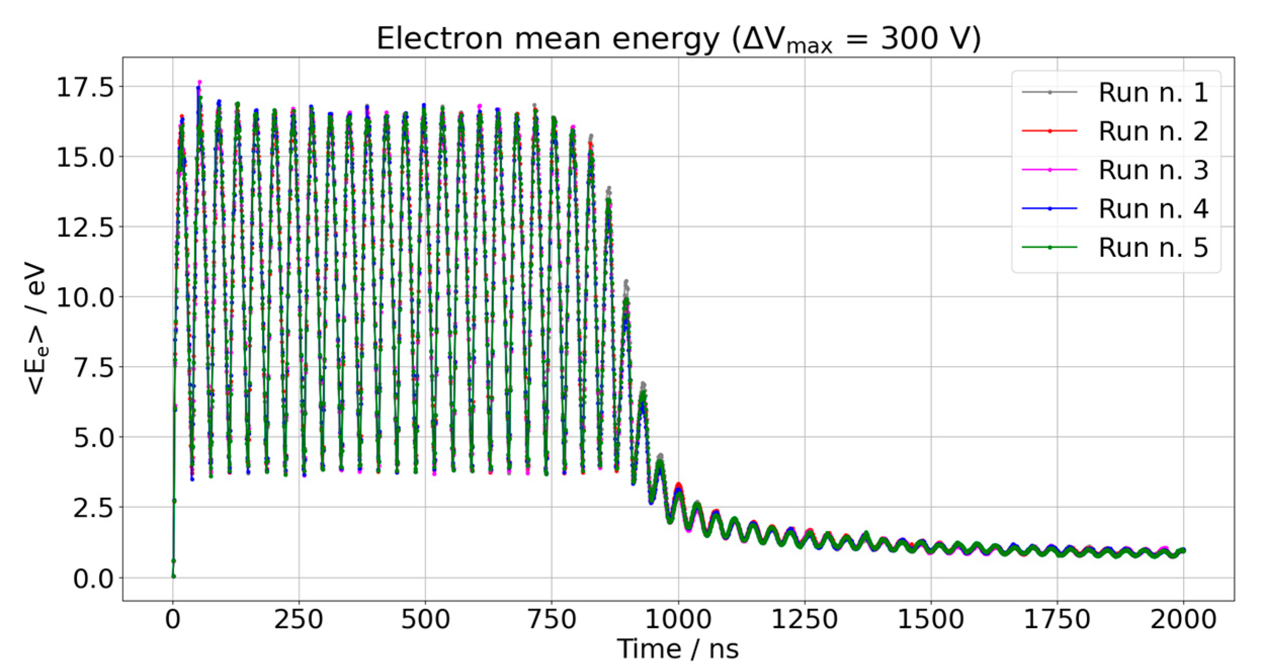
3.2. Electron Mean Energy

The mean energy of the electrons is shown as a function of time in Figure 2, for peak voltages (a) in range 150–350 V, and (b) 100, 400 V. In this case, similarly to the electron density, a dramatic change of behavior was observed separating two regimes, for peak bias voltages in range 150–350 V, while for bias voltages of 100 and 400 V the first regime only was observed. In the first regime, a strongly oscillating behavior of the electron mean energy was apparent, with an approximately constant amplitude increasing with the peak bias voltage, as seen in Figure 2a,c. In the second regime the mean electron energy started to fall, in terms of both the oscillation amplitude and the mean value, eventually reaching a finale state in which the oscillation ranged between 0.7 and 1.3 V depending on the peak bias voltage; as seen in Figure 2d, reporting the last 100 ns of simulated time. The time required for the transition between the two regimes reduced as the peak bias voltage increased from 150 to 250 V, but then increased for 300 and 350 V, consistent with observations for the electron density.

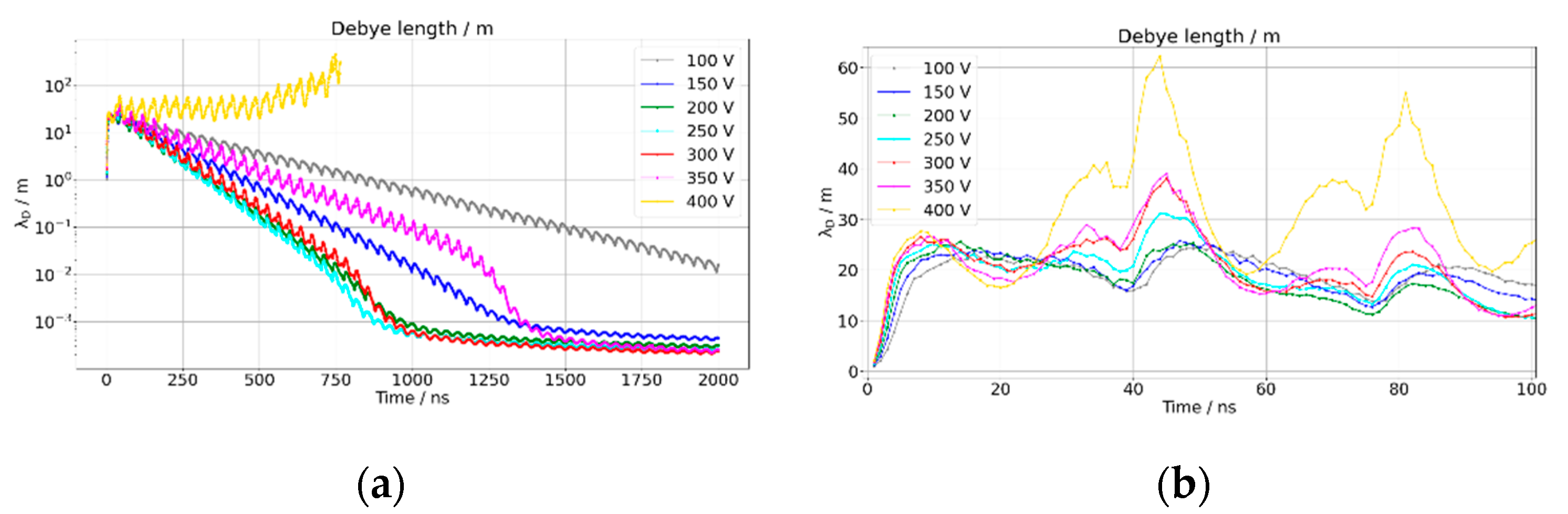
3.3. Debye Length

Figure 3a shows the time evolution of the Debye length (calculated from the electron density and mean energy by means of Equation (A3)) during the simulation for peak bias voltages in the range 100–400 V, in a semilogarithmic scale. Figure 3b shows a zoom of the time region up to 100 ns in a linear scale. The semilogarithmic plot shows a separation between two regimes, as already observed for the plasma density and the electron mean energy, for all the peak bias voltages except 100 and 400 V. In the first regime, an exponential decrease of λ_D with time (appearing as a linear decrease in the semilogarithmic plot) was observed, modulated by an oscillating behavior. This is to be expected, as the electron mean energy in this region of simulation time was oscillating around a constant value, while the electron density showed an exponential increase; λ_D is proportional to the square root of their ratio (Equation (A3)). The zoom on the first 100 ns shows the oscillating behavior, the amplitude of which increased with the peak bias voltage. However, this increase was much more intense from 350 to 400 V, where we observe a doubling of the Debye length peak value.

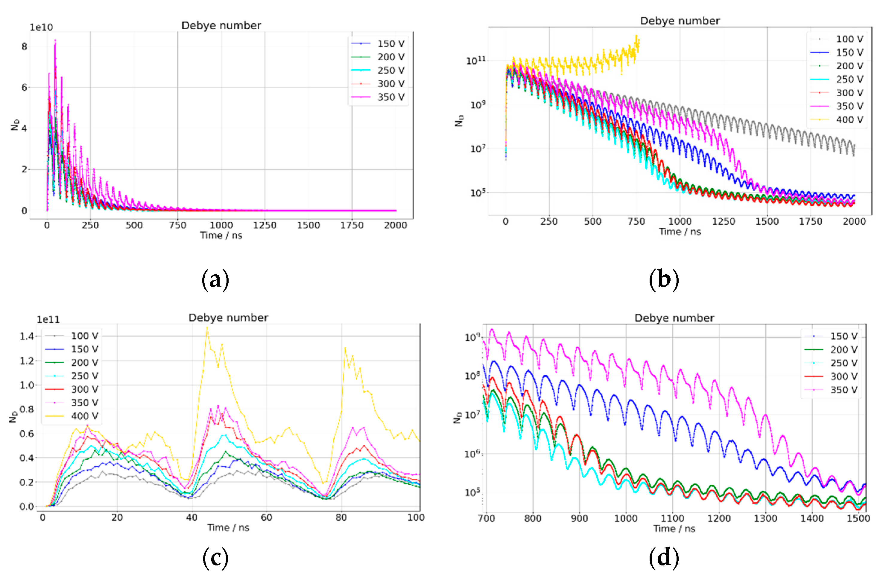
3.4. Debye Number

The time evolution of the Debye number N_D, which was calculated from the electron density and mean energy by means of Equation (A4), is shown in Figure 3 using (a) linear and (b) semilogarithmic scales. Zoomed graphs are also provided of (c) the first 100 ns in linear scale and (d) the 700–1500 ns range in semilogarithmic scale. The Debye number is commonly defined as the mean number of electrons comprised in a sphere having a radius equal to the Debye length, and values of N_D much greater than unity are usually associated with strong collective behavior of the electrons [22]. It is interesting to observe that, in the situation under consideration, the N_D value was already quite high (N_D = 10⁶) at the beginning of the simulation, then increased by several orders of magnitude during the first half of the RF cycle, as seen in Figure 4b,c. This can be explained by the fact that the mathematical expression of N_D (Equation (A4)), depends strongly on the electron energy, which increased considerably during the first half of the RF cycle, as shown in Figure 2, and depends much less on the electron density. After this initial rise, except at the 400 V peak bias voltage, the N_D value oscillated around an exponentially decreasing mean value (appearing as decreasing linear behavior in the semilogarithmic scale), with a change of slope in the region between 750 nm and 1 μs.

3.5. Plasma Frequency

The evolution of the plasma frequency ν_P (calculated from the electron density and mean energy by means of Equation (A5)) with the simulated time is shown in Figure 5 in (a) linear and (b) semilogarithmic scales. Zoomed graphs in semilogarithmic scale of (c) the first 100 ns in linear scale, and (d) the 700–1500 ns window (for peak bias voltages in range 150–350 V only) are also shown. The presence of two regimes is clearly visible, especially in graphs of Figure 5a,d, as well as the change of the time required for the onset of the second regime. In fact, increasing the peak bias voltage from 150 to 250 V, the regime transition shifted to shorter times, but when increasing further to 300 and 350 V, it began to shift to longer times. The first 100 ns of simulated time showed that for peak bias voltages in range 100–350 V, the amplitude of the oscillation increased with time, while for 400 V an opposite behavior was observed.

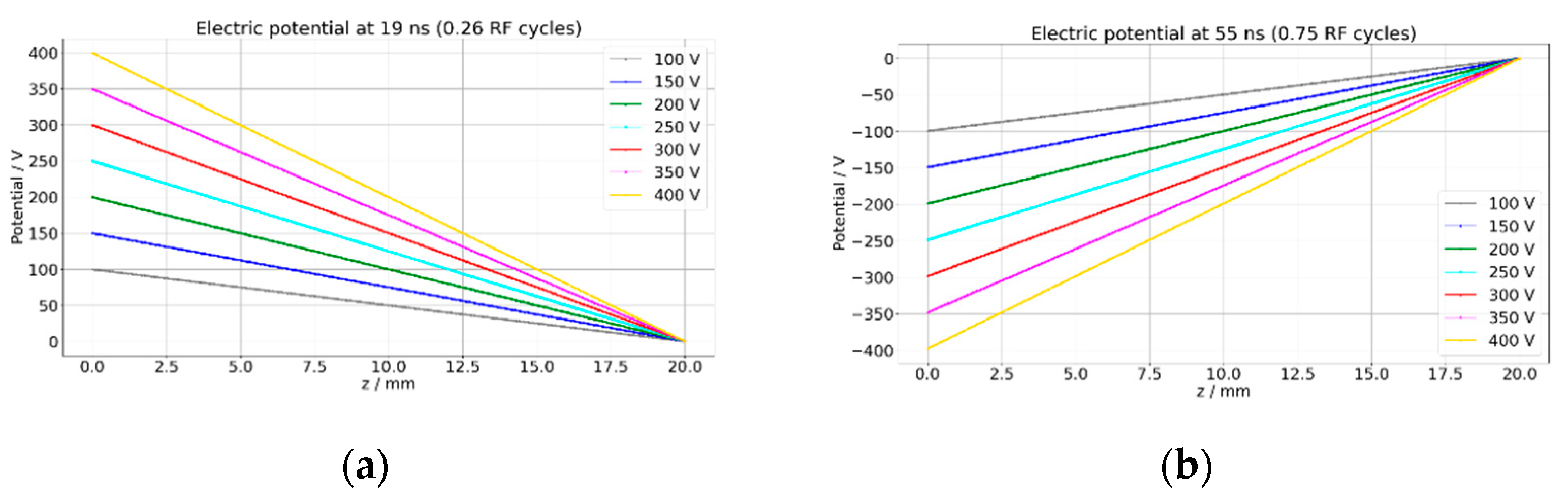
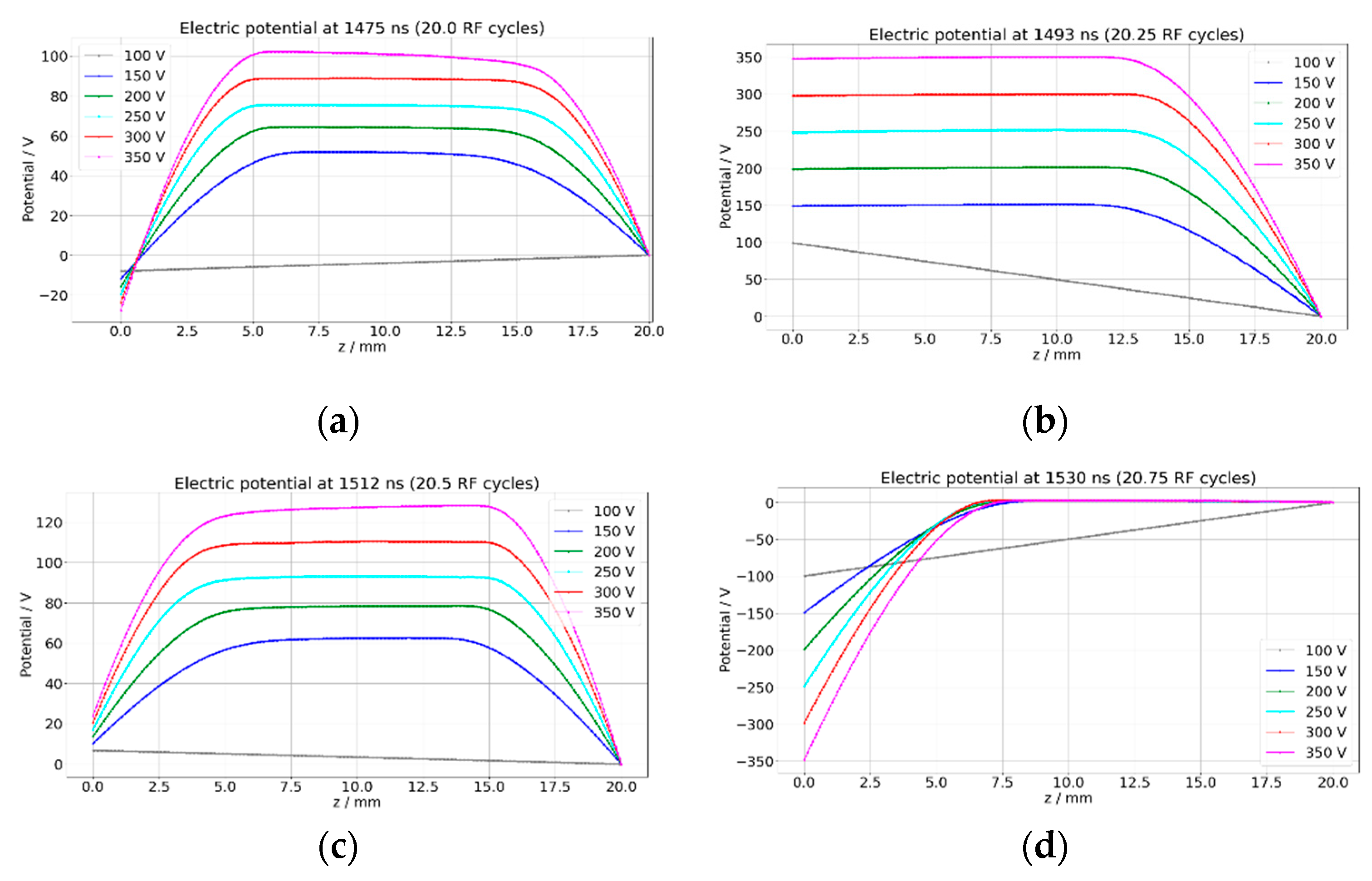
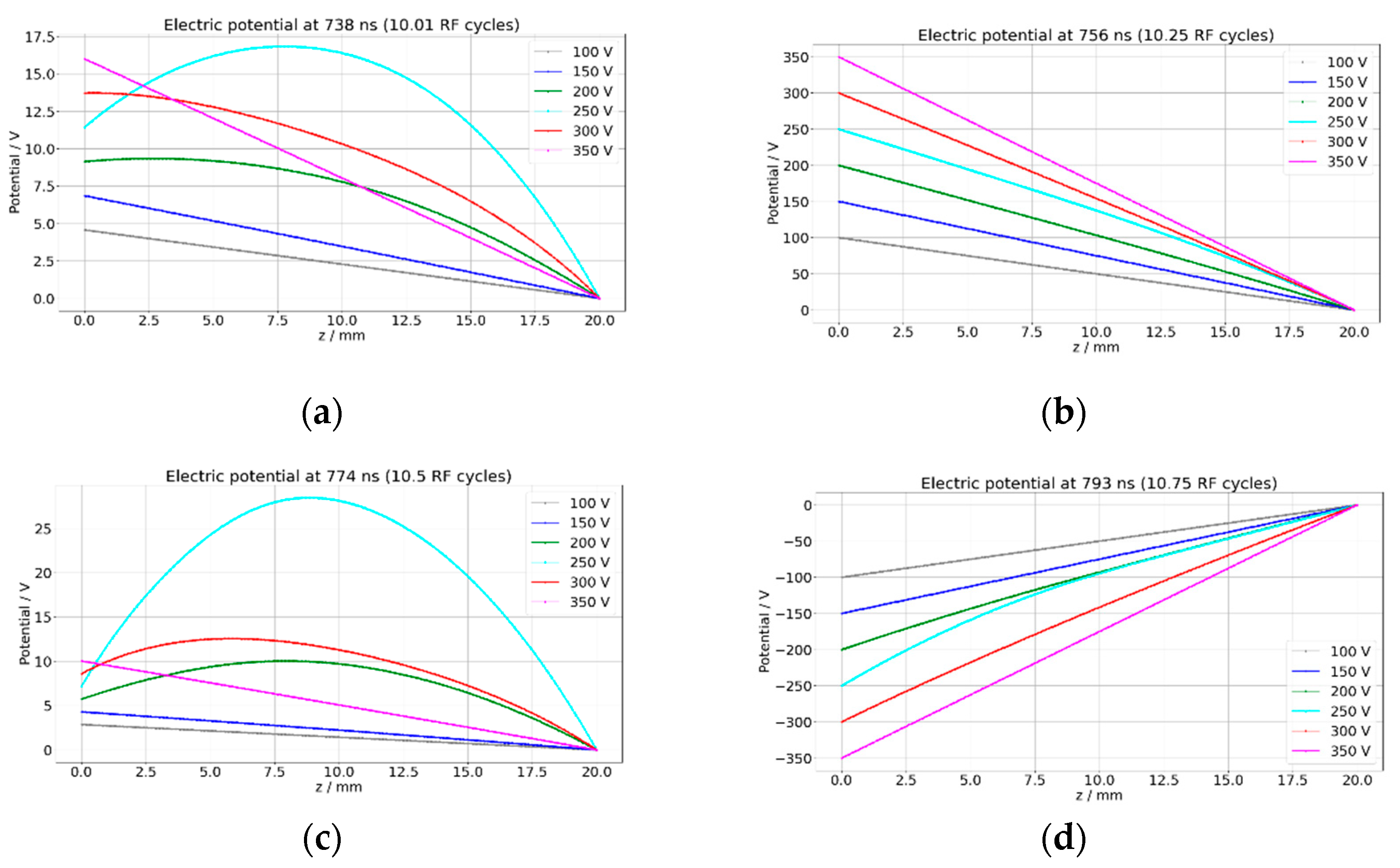
3.6. Spatial Distribution of the Electric Potential

The spatial distributions of the bias voltage calculated at different simulation times are shown in Figure 6, Figure 7 and Figure 8. Each plot shows the electric potential as a function of the z coordinate, which is the distance from the biased electrode along the normal direction, for the different values of the peak bias voltage. The grounded electrode was located at z = 20 mm and had a fixed potential of 0 V. Since the PIC method was implemented in one dimension only, the charge density, the electric potential, and the electric field were considered equal for all points sharing the same value of the z coordinate, i.e., the planar surfaces parallel to the electrodes.

Figure 6 shows the bias voltage calculated at ¼ and ¾ of the first RF cycle, when the electric bias on the polarized electrode reached maximum positive and maximum negative values, respectively. The absolute value of the voltage decreased from the biased electrode to the grounded one (z = 0 and z = 20 mm, respectively) with a constant slope, revealing a uniform electric field in the plasma volume. This result unsurprisingly shows that at the beginning of the simulation the charged particle density was too low to provide an effect on the electric field distribution, which was essentially dominated by the external bias.

Figure 7 shows the bias voltage calculated at the beginning, at ¼, at ½, and at ¾ of the 10th RF cycle, corresponding to the time window between 738 and 793 ns. For peak bias voltages of 100, 150, and 350 V, the potential changed linearly with z, showing a uniform electric field. Instead, for 200, 250 and 300 V, a bending of the voltage slope was clearly apparent, especially at the beginning and at ½ of the RF cycle (738 and 774 ns), much more pronounced for a peak bias of 250 V, showing that the charge density started to provide a contribution to the electric field of intensity comparable to the one of the external field. It is interesting to compare these results with the plots in Figure 1b,d, since the peak voltage values for which the bending is visible were those where, at the same of simulated time, the transition between the two regimes of plasma density increase had already begun to take place.

Figure 8 shows the bias voltage calculated at the beginning, at ¼, at ½, and at ¾ of the 20th RF cycle, corresponding to the time window between 1475 and 1530 ns. In this case, a bending of the voltage distribution was clearly observed for all values of peak bias voltage between 150 and 350 V, but not 100 V. If we compare again this result with the plots in Figure 1b,d, we can observe that in this time window the electron density time evolution had completed the transition from the exponential to the linear regime for all peak values except 100 V (not including 400 V, for which the time evolution had already stopped).

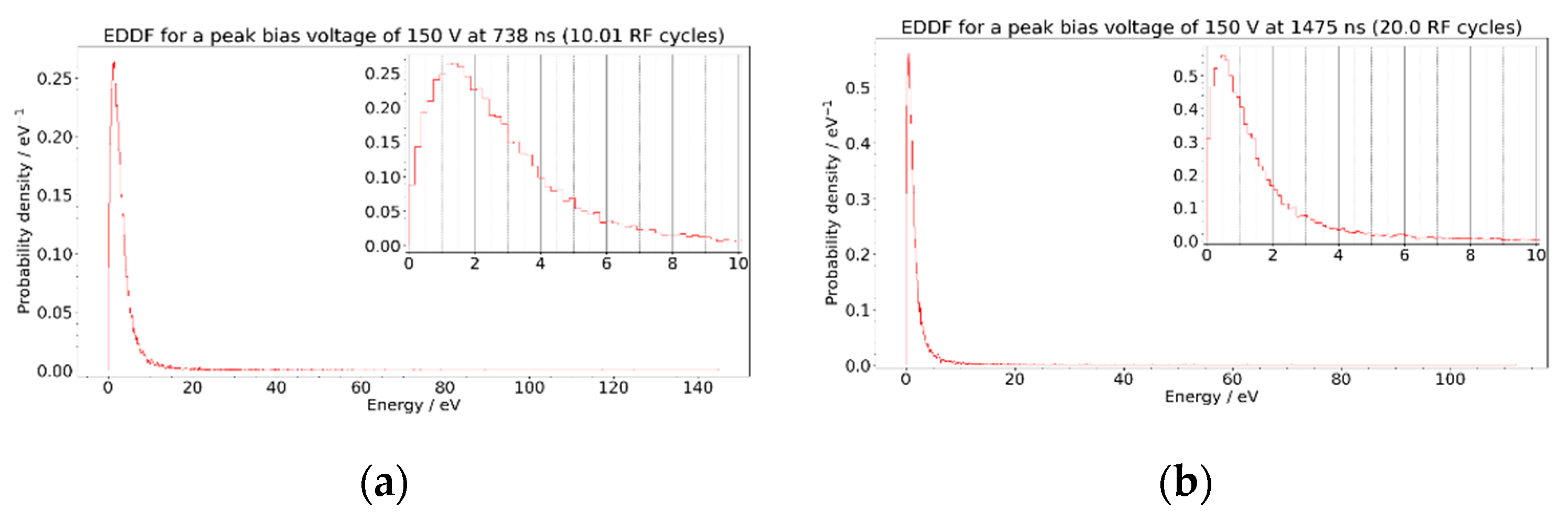
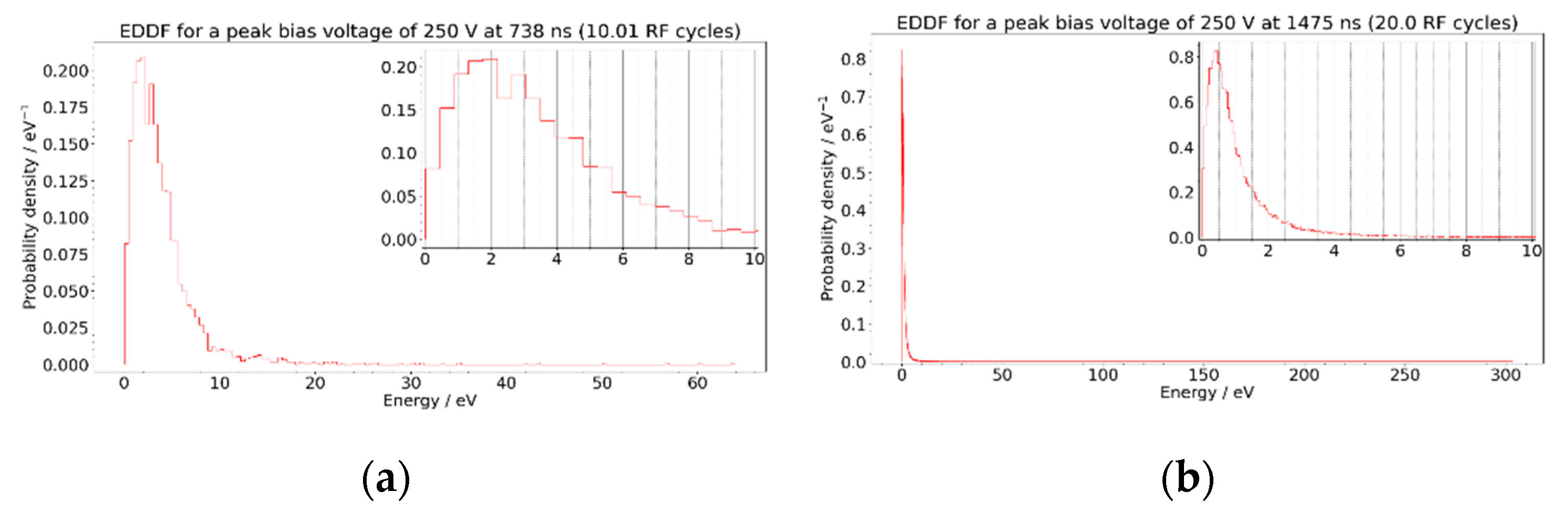
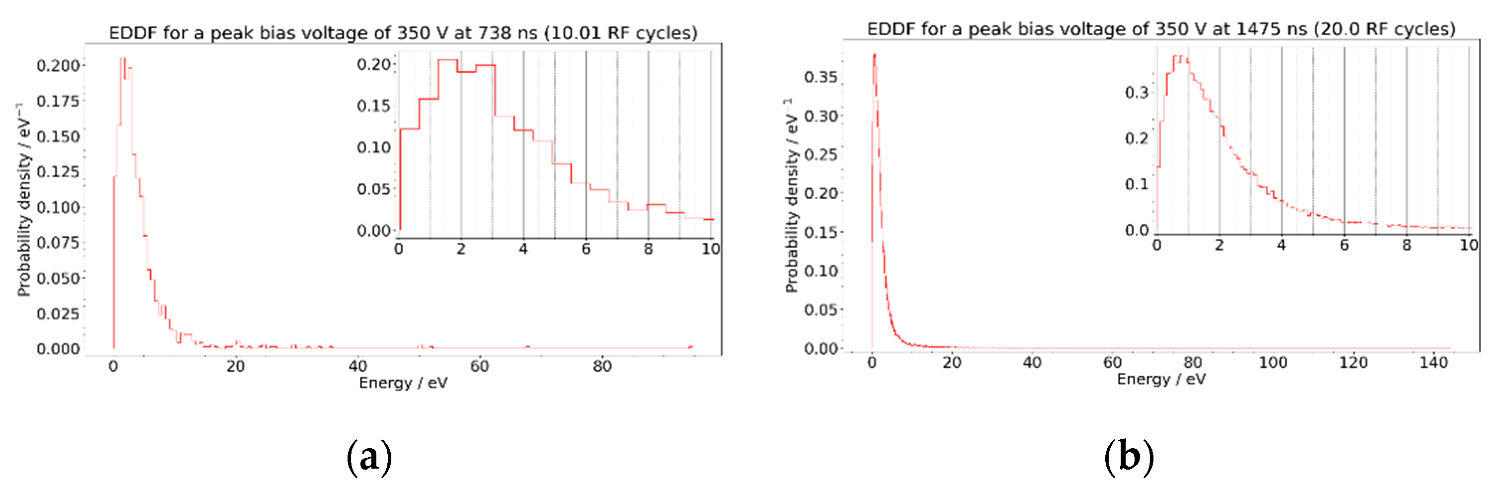
3.7. Electron Energy Distribution Functions

Figure 9, Figure 10 and Figure 11 show EEDFs evaluated at the beginning of the 10th and the 20th RF cycles, for peak bias voltages of 150, 200, and 250 V respectively, with an inset containing a zoom of the 0–10 eV region, added in order to make the peak position more readable. Figure 9 shows that, for a peak bias voltage of 150 V, there is a small change in the EEDF from the 10th to the 20th RF cycle, with a shift of the peak position towards a lower energy. A more pronounced change is visible in Figure 10, for a peak bias voltage of 250 V: although the peak moves at lower energy, we can observe an increase of the high-energy tail, with an increase of the maximum electron energy. Figure 11, related to a peak bias voltage of 350 V, shows a less peaked shape of the EEDFs and, again, a shift of the peak towards lower energy from the 10th to the 20th RF cycle, together with an increase of the high-energy tail.

3.8. Variability of the Simulation Results

The discharge simulation for the peak voltage of 300 V was repeated 5 times to estimate the variation of the results within different runs with the same parameters. The plots of the electron density time evolution for the different simulation runs are shown in Figure 12 in linear (a) and semilogarthmic (b) scale, while the mean electron energy plots are shown in Figure 13. The variation shown by the graphs is clearly much lower than the one obtained in simulation runs when the bias peak value was varied (Figure 1a,b and Figure 2a).

4. Discussion

The main goal of this work is to give a contribution to the understanding of the processes involved in the ignition mechanism of low pressure RF-CCP discharges. The most evident result obtained by these simulations is the presence, during the first discharge microsecond in the chosen discharge conditions, of a transition between two regimes, characterized by different behaviors of the plasma parameters with time. While the electron density changes from an exponential increase to a linear one (both of them modulated by oscillations), the electron mean energy changes from a strongly oscillating behavior around a constant mean value, with an amplitude depending on the peak voltage bias, to an oscillation with much lower amplitude and mean value, which is similar for all the investigated peak bias voltages.

The other plasma parameters, such as Debye length, Debye number, and plasma frequency [23], reflect these behaviors, since they are calculated starting from the electron density and mean energy, as described in Appendix B. It is interesting to note that the Debye number rises to values greater than 10¹⁰ already during the first half RF cycle, but later it reduces to much lower values, especially after the transition to the second regime, which however are still greater than 10⁴. Since high values of the Debye number are usually considered associated with a collective behavior of charged particles [22], the simulation results suggest that, based on this parameter only, the charges should show a collective behavior starting from the very beginning. On the other hand, during the first RF cycle, the spatial distribution of the bias voltage does not show any sign of bending, revealing the absence of a significative self-consistent electric field, which appears with the transition between the two regimes only, as seen in Figure 6, Figure 7 and Figure 8.

At the beginning of the simulation, the plasma frequency ν_P is in the range 40–120 kHz, about two orders of magnitude lower then the RF frequency ν_RF= 13.56 MHz, so the electrons should not be able to provide a quick enough response to the variation of the external bias [23]. According to the results shown in Figure 5b, the transition between the two regimes is always associated with values of the plasma frequency of the order of 100 MHz, about ten times ν_RF. These results suggest that the plasma frequency has a role in driving the transition between the two regimes observed. In fact, as the plasma frequency rises, the difference in the behavior of electrons and ions becomes more important, since the latter have a much higher mass, that strongly limits their mobility. The transition between the two regimes seems to reflect the onset of a charge accumulation, which is associated with the development of an internal electric field, as seen in Figure 6, Figure 7 and Figure 8. The strong reduction of the electron mean energy in the second regime could be explained considering that a considerable fraction of the energy, that in the first regime is accumulated in the electron kinetic energy, is transferred in the internal electric field developed by the charge separation.

The formation of a self-consistent electric field is observed during the 10th RF cycle, for the 200, 250 and 300 V RF amplitudes, by the bending of the voltage spatial distributions shown in Figure 7. For these values of the peak bias voltage, the transition between the two regimes happens between 800 and 900 ns, as is visible in Figure 1b,d, so the deformation of the potential distribution seems to be somehow predictive of the transition. The presence of a non uniform electric field can be associated with the development of a spatial charge, which is typically a result of the difference between the behavior of ions and electrons in the discharge [19,22]. In fact, due their higher mass, ions are much less able to follow the electric field variation, compared to electrons, and this difference leads to the accumulation of positive charges in the central region of the discharge. As the electron and ion density rise, the intensity of the electric field produced by this charge accumulation increases, eventually becoming comparable to the external one, thus producing a deformation of the potential spatial distribution.

The time required for the transition between the two regimes shows an interesting behavior, since it reduces as the peak bias voltage ∆V_max is risen from 100 to 250 V, but it increases when a further rise of ∆V_max to 300 and 350 V is applied, as is clearly visible in Figure 1a. Moreover, at 400 V no increase is observed at all and, after a few RF cycles, the simulation shows a decrease of the electron density towards zero. The same consideration applies to the slope of the electron density rise in the semilogarithmic plots of Figure 1b,d. This behavior may seem inconsistent, since, in the first regime, the amplitude of the mean electron energy oscillations increases considerably with the peak bias voltage, reaching a value as high as 20 eV for 400 V. Since the efficiency of the electron-impact ionization processes of Ar increases with the electron energy up to about 100 eV [20], one could expect the higher values of the mean electron energy to be always associated with a more rapid increase of the electron density.

A possible explanation of this behavior could be related to the time required for the electrons to move between the electrodes. In fact, a free electron produced in the discharge can contribute to the ionization processes while it is accelerated toward the electrode that, at that time, has the higher electric potential. During an half RF period, it is always accelerated toward the same electrode, since the electric field is changing in intensity, but not in direction. Obviously, a stronger electric field produces a higher electron speed, increasing the ionization efficiency (at least up to energies of about 100 eV). However, if the electron becomes too fast, it may reach the electrode before the electric field direction changes, being removed from the discharge. Instead, if the electric field inversion happens before the electron has been absorbed, it starts to be accelerated in the opposite direction, and may not be removed from the discharge, continuing to contribute to the ionization processes. For these reasons, an excessive electron energy, and consequently speed, could increase the the probability that an electron is absorbed before the inversion of the electric field takes place. As an example, considering the peak bias voltage of 350 V, the electron mean energy averaged over the first half RF cycle (1–37 ns) is 11.9 eV, which gives a time to move between the two electrodes of about 9.8 ns, which is about 26% of an half RF cycle (τ_RF/2 = 37 ns). Since a certain fraction of the electrons has an energy higher than the mean value, as can be seen in the EEDF reported in Figure 9, Figure 10 and Figure 11, there is a considerable number of them that has a high probability of being absorbed by the electrodes.

The previous considerations could explain why, in the second regime observed, the the slope of the linear electron density always rises with the peak bias voltage, as seen in Figure 1a, for 300 V and 350 V also. In fact, after the transition between the two regimes has been completed, the amplitude and mean value of the <E_e> oscillations drop dramatically, as seen in Figure 2a,d. Considering again a 350 V peak bias voltage, the value of <E_e> averaged over the last simulated half RF cycle (1954–1991 ns) is 1 eV, corresponding to a time required to move between the electrodes of 33.7 ns, about 91% of an half RF cycle. It is possible to presume that, in these conditions, the number of electrons that are removed from the discharge by electrode absorption is much lower compared to the situation of the first regime.

As an additional consideration, the onset of a charge separation is usually associated with the formation of sheath structures near the electrodes, and the electric potential distribution shown in Figure 8 seems to confirm the sheaths presence, with the formation of potential barriers at both the electrodes. These may prevent the electrons with energy lower than a certain threshold from reaching the electrodes, thus avoiding their absorption. Since this kind of structure is not present in the potential distribution during the first regime (Figure 6 and Figure 7), it could be considered as an additional mechanism increasing the lifetime of electrons in the discharge during the second regime.

5. Conclusions

Within the limits of the model used, the simulation of the first 2 μs of a low pressure (66.6 Pa) Ar RF-CCP discharge with peak bias voltages in range 100–400 V showed the presence of two regimes, characterized by an exponential and linear increase of the electron density with time, respectively. The behavior of the electron mean energy changes also considerably between the two regimes: while in the first one it shows oscillations with peak values that reach 20 eV for 400 V peak bias voltage, in the second regime the oscillation are strongly reduced in both amplitude and mean value, which becomes of the order of 1 eV. The time required for the transition between the two regimes is reduced with the peak bias voltage rise up to 250 V, but increasing it further to 300 and 350 V produces the opposite effect, and for 400 V there is no transition at all.

References

- Chabert, P.; Tsankov, T.V.; Czarnetzki, U. Foundations of capacitive and inductive radio-frequency discharges. Plasma Sources Sci. Technol. 2021, 30, 024001. [Google Scholar] [CrossRef]
- Ostrikov, K.; Xu, S.; Huang, S.Y.; Levchenko, I. Nanoscale surface and interface engineering: Why plasma-aided? Surf. Coat. Tech. 2008, 202, 5314–5318. [Google Scholar] [CrossRef]
- Marchack, N.; Buzi, L.; Farmer, D.B.; Miyazoe, H.; Papalia, J.M.; Yan, H.; Totir, G.; Engelmann, S.U. Plasma processing for advanced microelectronics beyond CMOS. J. Appl. Phys. 2021, 130, 080901. [Google Scholar] [CrossRef]
- Xiao, S.Q.; Xu, S.; Ostrikov, K. Low-temperature plasma processing for Si photovoltaics. Mat. Sci. Eng. R 2014, 78, 1–29. [Google Scholar] [CrossRef]
- Granqvist, C.G. Electrochromics for smart windows: Oxide-based thin films and devices. Thin Solid Film. 2014, 564, 1–38. [Google Scholar] [CrossRef]
- Hammer, T. Atmospheric Pressure Plasma Application for Pollution Control in Industrial Processes. Contrib. Plasma Phys. 2014, 54, 187–201. [Google Scholar] [CrossRef]
- Vasudev, M.C.; Anderson, K.D.; Bunning, T.J.; Tsukruk, V.V.; Naik, R.R. Exploration of Plasma-Enhanced Chemical Vapor Deposition as a Method for Thin-Film Fabrication with Biological Applications. ACS Appl. Mater. Interfaces 2013, 5, 3983–3994. [Google Scholar] [CrossRef]
- Weltmann, K.D.; von Woedtke, T. Plasma medicine-current state of research. Plasma Phys. Control. Fusion 2017, 59, 014031. [Google Scholar] [CrossRef]
- Cha, S.; Park, Y.-S. Plasma in dentistry. Clin. Plasma Med. 2014, 2, 4–10. [Google Scholar] [CrossRef]
- Wang, X.-Y.; Liu, J.-R.; Liu, Y.-X.; Donko, Z.; Zhang, Q.-Z.; Zhao, K.; Schulze, J.; Wang, Y.N. Comprehensive understanding of the ignition process of a pulsed capacitively coupled radio frequency discharge: The effect of power-off duration. Plasma Sources Sci. Technol. 2021, 30, 075011. [Google Scholar] [CrossRef]
- Ma, F.-F.; Zhang, Q.-Z.; Schulze, J.; Sun, J.-Y.; Wang, Y.-N. Temporal evolution of plasma characteristics in synchronized dual-level RF pulsed capacitively coupled discharge. Plasma Sources Sci. Technol. 2021, 30, 105018. [Google Scholar] [CrossRef]
- Su, Z.-X.; Shi, D.-H.; Liu, Y.-X.; Zhao, K.; Gao, F.; Wang, Y.-N. Radially-dependent ignition process of a pulsed capacitively coupled RF argon plasma over 300 mm-diameter electrodes: Multi-fold experimental diagnostics. Plasma Sources Sci. Technol. 2021, 30, 125013. [Google Scholar] [CrossRef]
- Darnon, M.; Cunge, G.; Braithwaite, N.J. Time-resolved ion flux, electron temperature and plasma density measurements in a pulsed Ar plasma using a capacitively coupled planar probe. Plasma Sources Sci. Technol. 2014, 23, 025002. [Google Scholar] [CrossRef]
- Denysenko, I.B.; von Wahl, E.; Mikikian, M.; Berndt, J.; Ivko, S.; Kersten, H.; Kovacevic, E.; Azarenkov, D.M.; Cunge, G.; Braithwaite, N.J. Plasma properties as function of time in Ar/C2H2 dust-forming plasma. J. Phys. D Appl. Phys. 2020, 53, 135203. [Google Scholar] [CrossRef]
- Schulze, J.; Derzsi, A.; Dittmann, K.; Hemke, T.; Meichsner, J.; Donko, Z. Ionization by Drift and Ambipolar Electric Fields in Electronegative Capacitive Radio Frequency Plasmas. Phys. Rev. Lett. 2011, 107, 275001. [Google Scholar] [CrossRef]
- Schmidt, N.; Schulze, J.; Schungel, E.; Czarnetzki, U. Effect of structured electrodes on heating and plasma uniformity in capacitive discharges. J. Phys. D Appl. Phys. 2013, 46, 505202. [Google Scholar] [CrossRef]
- Behounek, F.; Kletschka, J.A. Ionization of Air in an Air-conditioned Building. Nature 1938, 142, 956. [Google Scholar] [CrossRef]
- Suchanowski, A.; Wiszniewski, A. Changes in Ion Concentration in the Air during the Breathing Process of a Human Being. Pol. J. Environ. Stud. 1999, 8, 259–263. [Google Scholar]
- Donkó, Z.; Derzsi, A.; Máté Vass, M.; Horváth, B.; Wilczek, S.; Hartmann, B.; Hartmann, P. eduPIC: An introductory particle based code for radio-frequency plasma simulation. Plasma Sources Sci. Technol. 2021, 30, 095017. [Google Scholar] [CrossRef]
- Raju, G.G. Electron-atom Collision Cross Sections in Argon: An Analysis and Comments. IEEE Trans. Dielectr. Electr. Insul. 2004, 11, 649–673. [Google Scholar] [CrossRef]
- Bogaerts, A.; Van Straaten, M.; Gijbel, R. Monte Carlo simulation of an analytical glow discharge: Motion of electrons, ions and fast neutrals in the cathode dark space. Spectrochim. Acta 1995, 50B, 179–196. [Google Scholar] [CrossRef]
- Schumacher, U. Basics of Plasma Physics. In Lecture Notes in Physics-Plasma Physics; Dinklage, A., Klinger, T., Marx, G., Schweikhard, L., Eds.; Springer: Berlin/Heidelberg, Germany, 2005; pp. 3–20. [Google Scholar]
- Von Keudell, A.; Schulz-von der Gathen, V. Foundations of low-temperature plasma physics-an introduction. Plasma Sources Sci. Technol. 2017, 26, 113001. [Google Scholar] [CrossRef]
- Pysica 0.2.0. Available online: https://pypi.org/project/pysica (accessed on 15 August 2022).
- GNU General Public License. Available online: https://www.gnu.org/licenses/gpl-3.0.html (accessed on 14 August 2022).
- Peterson, P. F2PY: A tool for connecting Fortran and Python programs. Int. J. Comput. Sci. Eng. 2009, 4, 296–305. [Google Scholar] [CrossRef]
- The GNU Fortran Compiler. Available online: https://gcc.gnu.org/onlinedocs/gfortran (accessed on 14 August 2022).
- Birdsall, C.K. Particle-in-Cell Charged-Particle Simulations, Plus Monte Carlo Collisions With Neutral Atoms, PC-MCC. IEEE Trans. Sci. 1991, 19, 65–85. [Google Scholar]