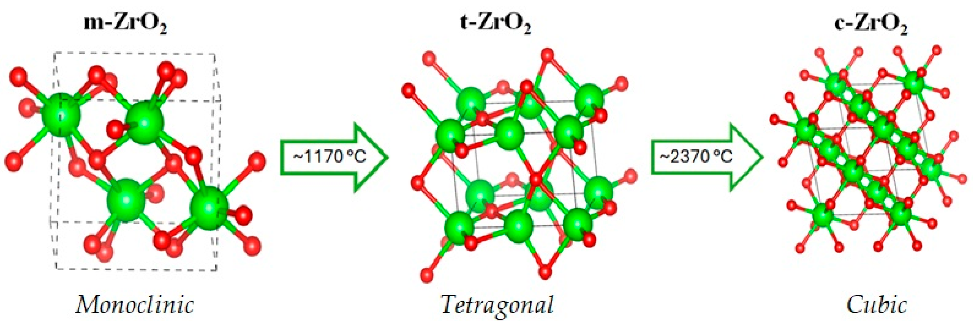
Figure 1.
The typical crystallographic structures of zirconium dioxide and the phase transition temperatures between them.
Figure 1.
The typical crystallographic structures of zirconium dioxide and the phase transition temperatures between them.
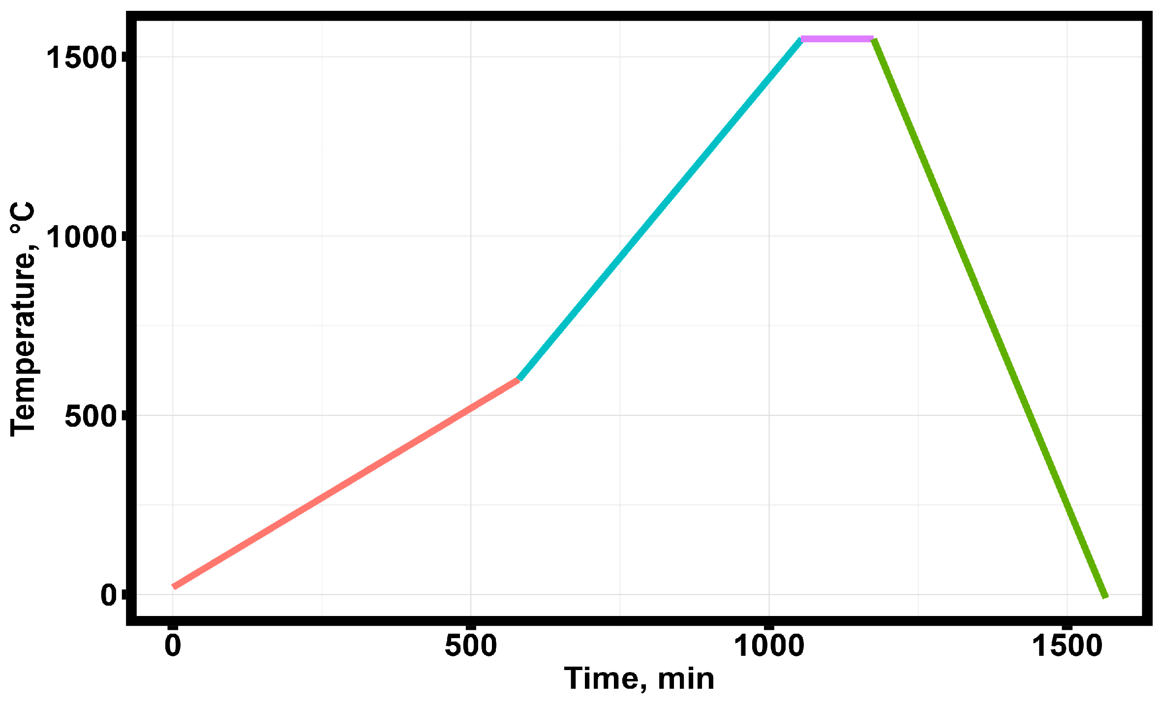
Figure 2.
Post-processing cycle of the printed samples.
Figure 2.
Post-processing cycle of the printed samples.
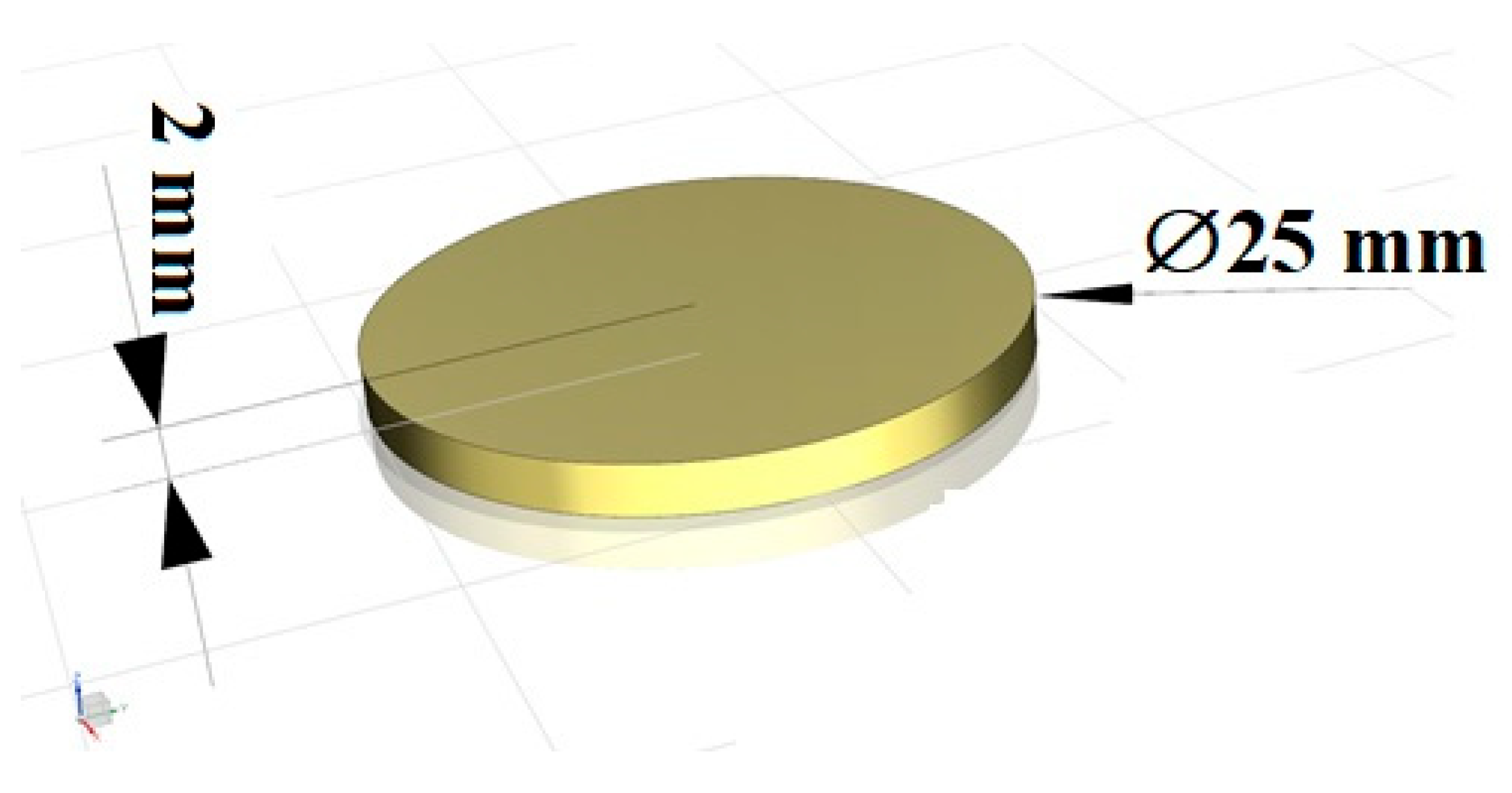
Figure 3.
Shape and dimensions of the blank produced by FDM printing technology from an extruded filament.
Figure 3.
Shape and dimensions of the blank produced by FDM printing technology from an extruded filament.
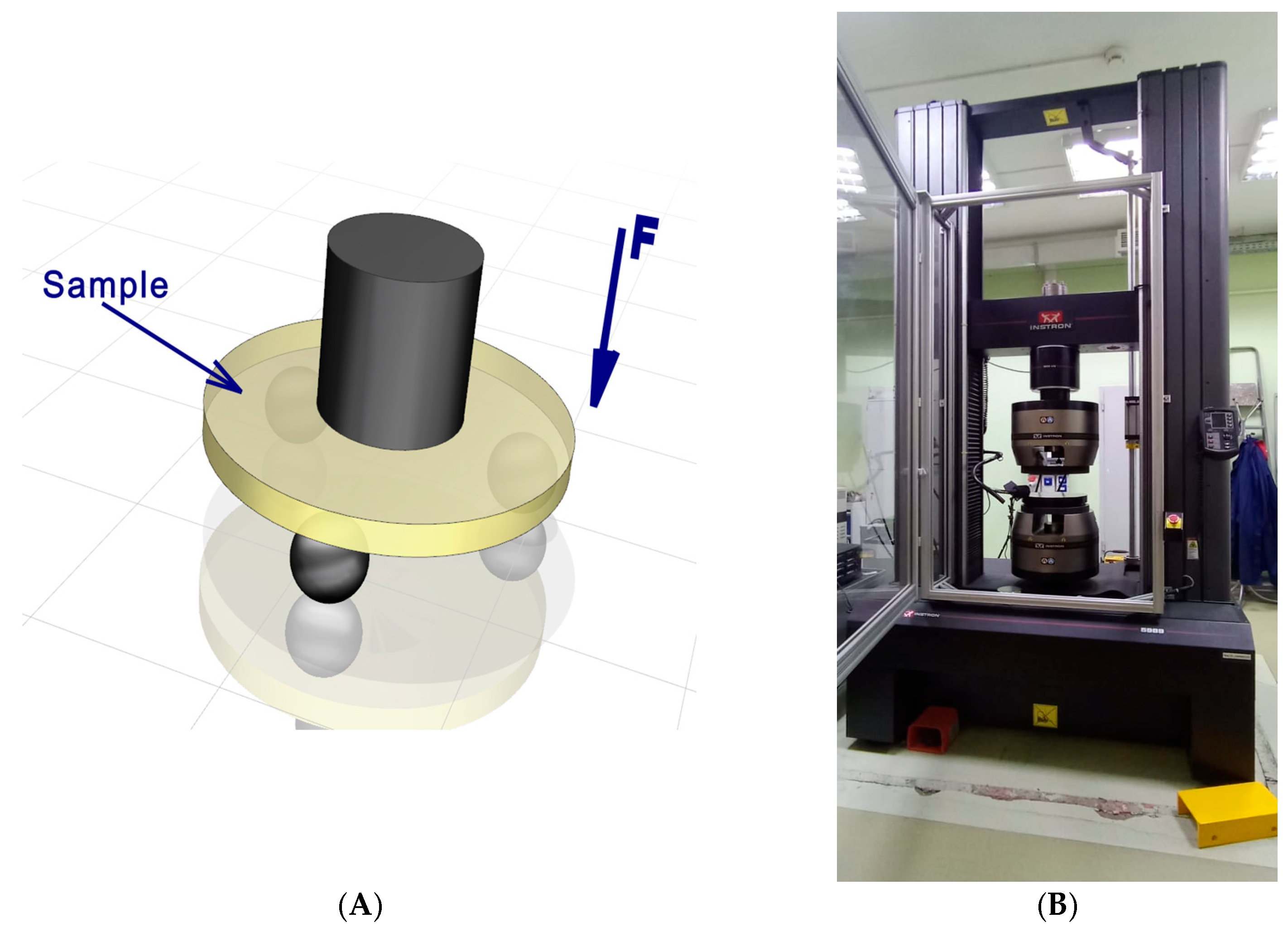
Figure 4.
(A) Schematic of the biaxial flexural test; (B) test equipment image.
Figure 4.
(A) Schematic of the biaxial flexural test; (B) test equipment image.
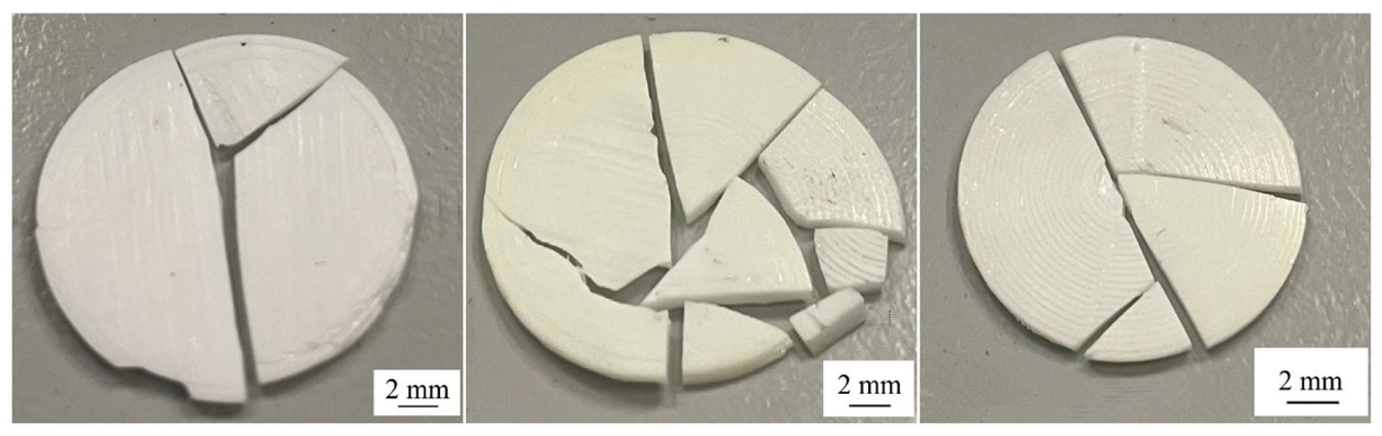
Figure 5.
Representative optical images of the sintered disks after biaxial testing.
Figure 5.
Representative optical images of the sintered disks after biaxial testing.
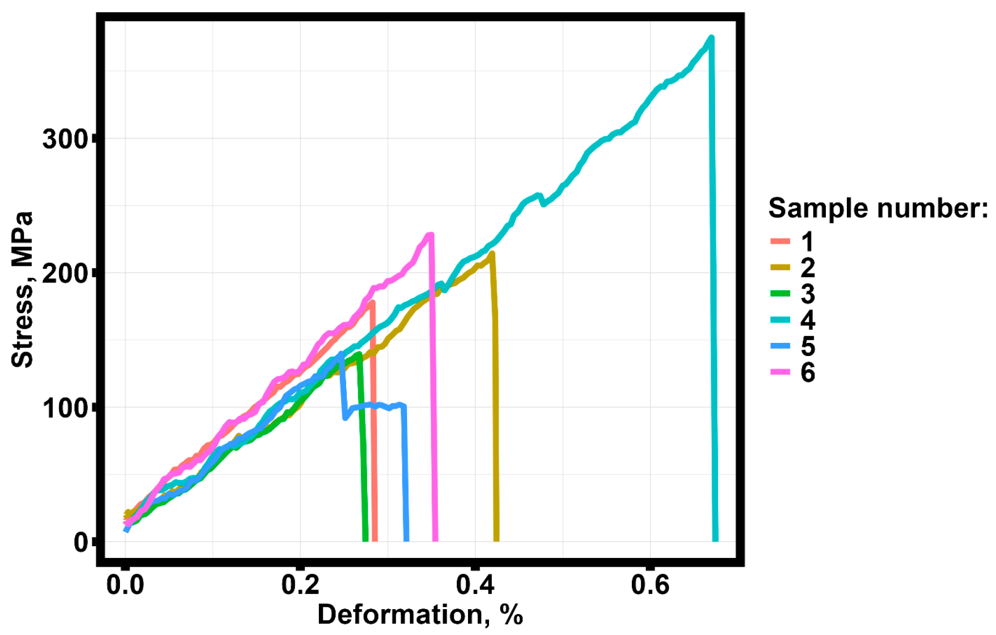
Figure 6.
Engineering stress–deformation diagram for the sintered samples obtained by the annealing of blanks produced by FDM printing technology with a filling layer thickness of 0.3 mm and a nozzle diameter of 0.6 mm.
Figure 6.
Engineering stress–deformation diagram for the sintered samples obtained by the annealing of blanks produced by FDM printing technology with a filling layer thickness of 0.3 mm and a nozzle diameter of 0.6 mm.
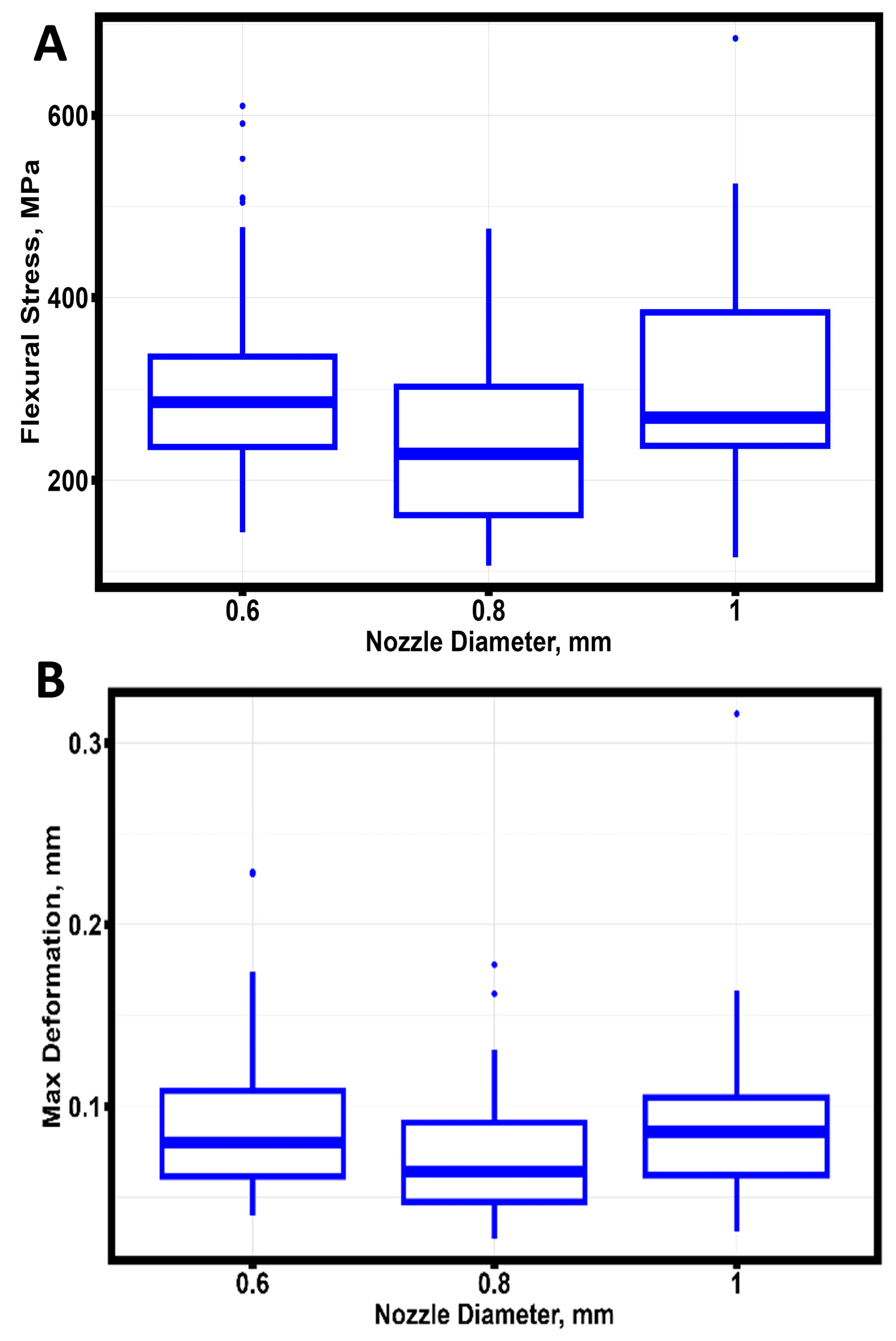
Figure 7.
The variation of the mechanical properties of the ceramic specimens in the biaxial test as a function of nozzle diameter. (A) Stress limit. (B) Deformation corresponding to the maximum force.
Figure 7.
The variation of the mechanical properties of the ceramic specimens in the biaxial test as a function of nozzle diameter. (A) Stress limit. (B) Deformation corresponding to the maximum force.
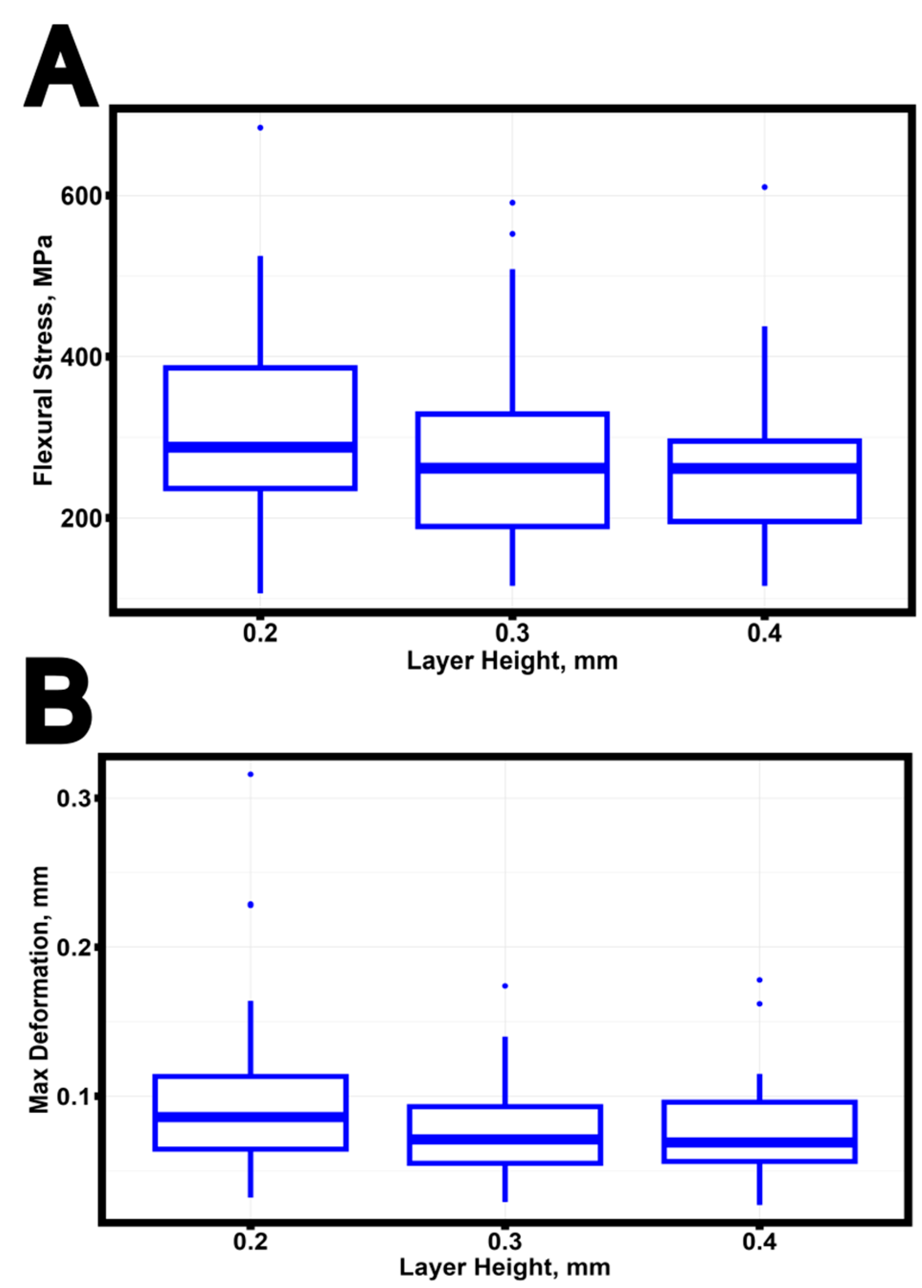
Figure 8.
The variation of the mechanical properties of the ceramic specimens in mechanical tests as a function of layer height in the FDM printing of the workpiece. (A) Stress limit. (B) Deformation corresponding to the maximum force.
Figure 8.
The variation of the mechanical properties of the ceramic specimens in mechanical tests as a function of layer height in the FDM printing of the workpiece. (A) Stress limit. (B) Deformation corresponding to the maximum force.
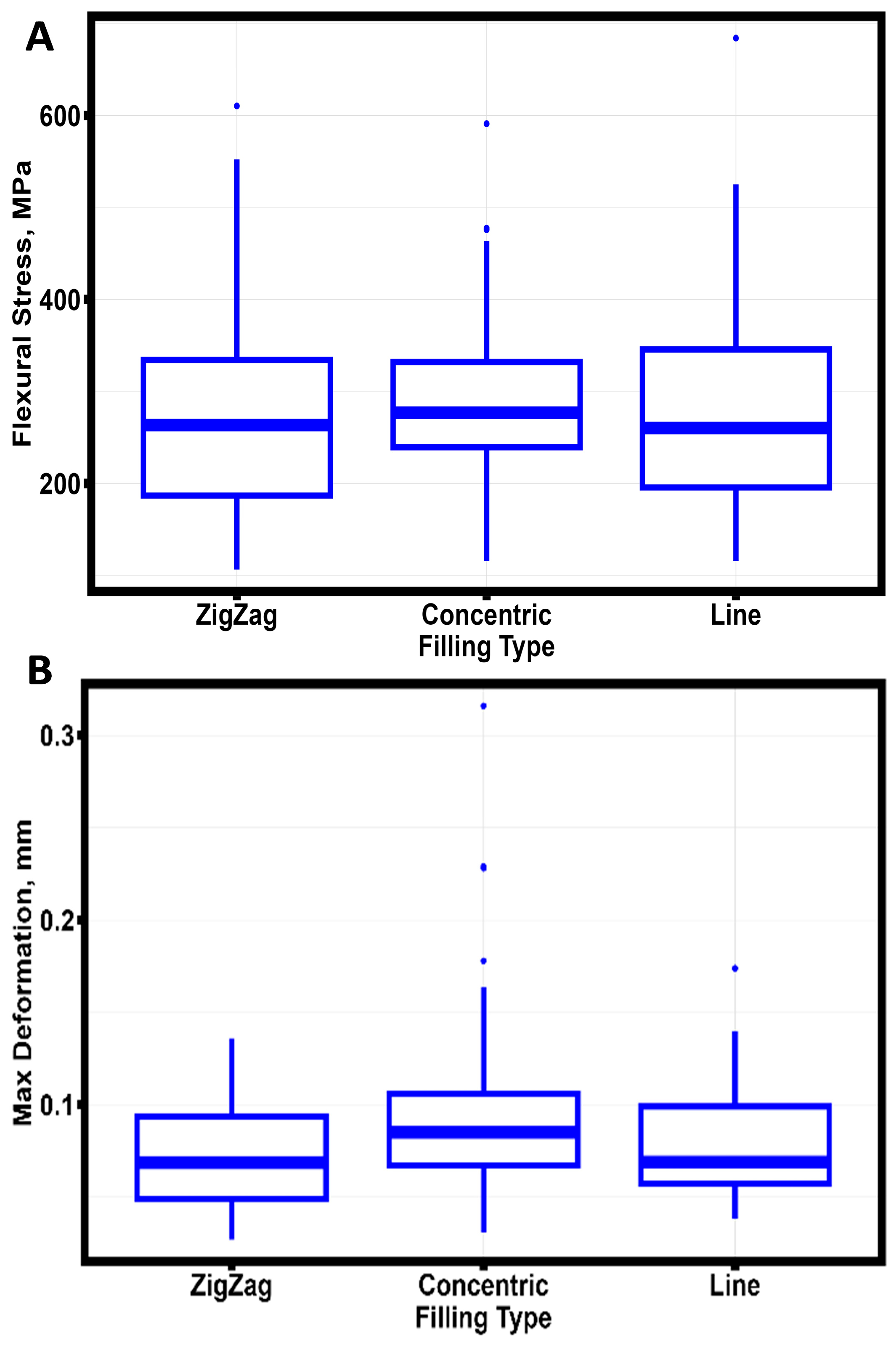
Figure 9.
The variation of the mechanical properties of ceramic specimens under biaxial loading depending on the type of filling during the FDM printing of the workpiece. (A) Stress limit. (B) Deformation corresponding to the maximum force.
Figure 9.
The variation of the mechanical properties of ceramic specimens under biaxial loading depending on the type of filling during the FDM printing of the workpiece. (A) Stress limit. (B) Deformation corresponding to the maximum force.
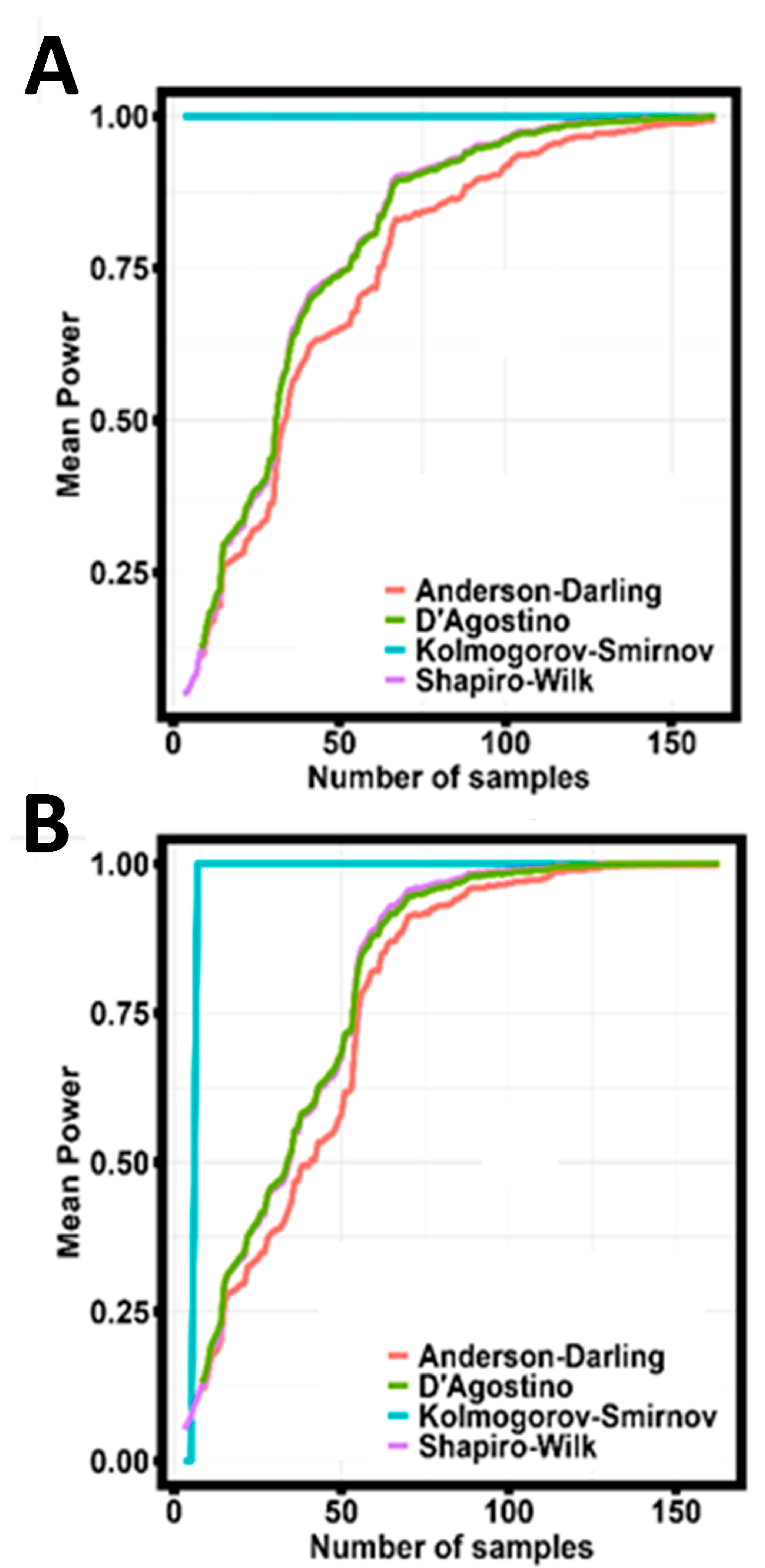
Figure 10.
The dependence of the average statistical power on the number of specimens tested. (A) Stress limit. (B) Strain corresponding to the maximum force.
Figure 10.
The dependence of the average statistical power on the number of specimens tested. (A) Stress limit. (B) Strain corresponding to the maximum force.
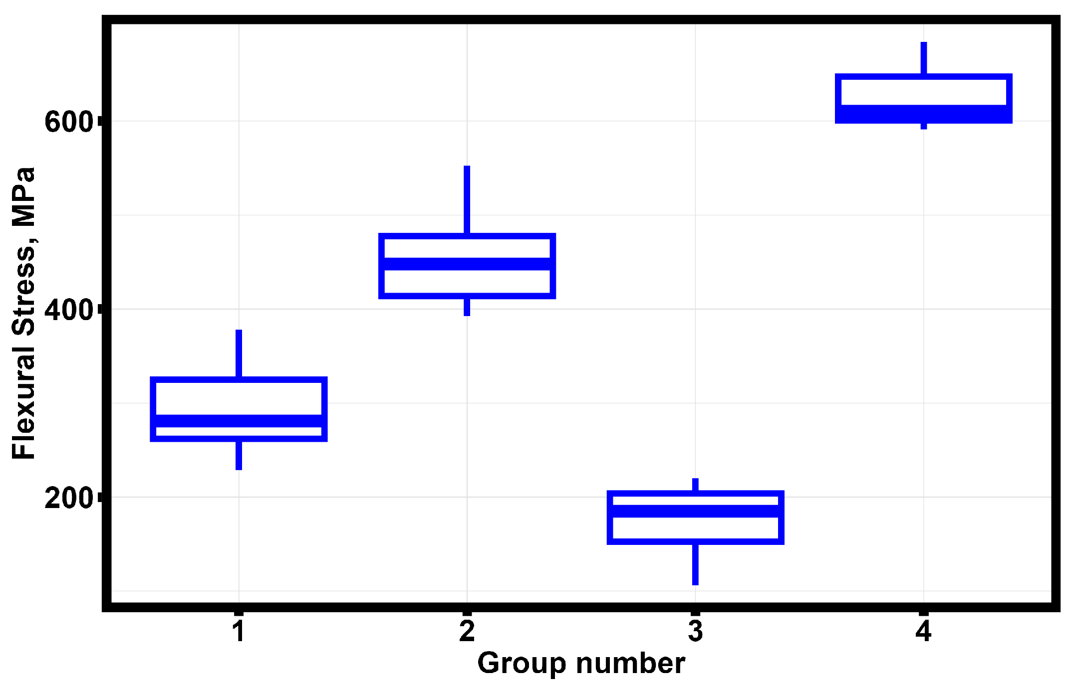
Figure 11.
The results of the stress classification of the zirconium oxide specimens subjected to flexural loading.
Figure 11.
The results of the stress classification of the zirconium oxide specimens subjected to flexural loading.
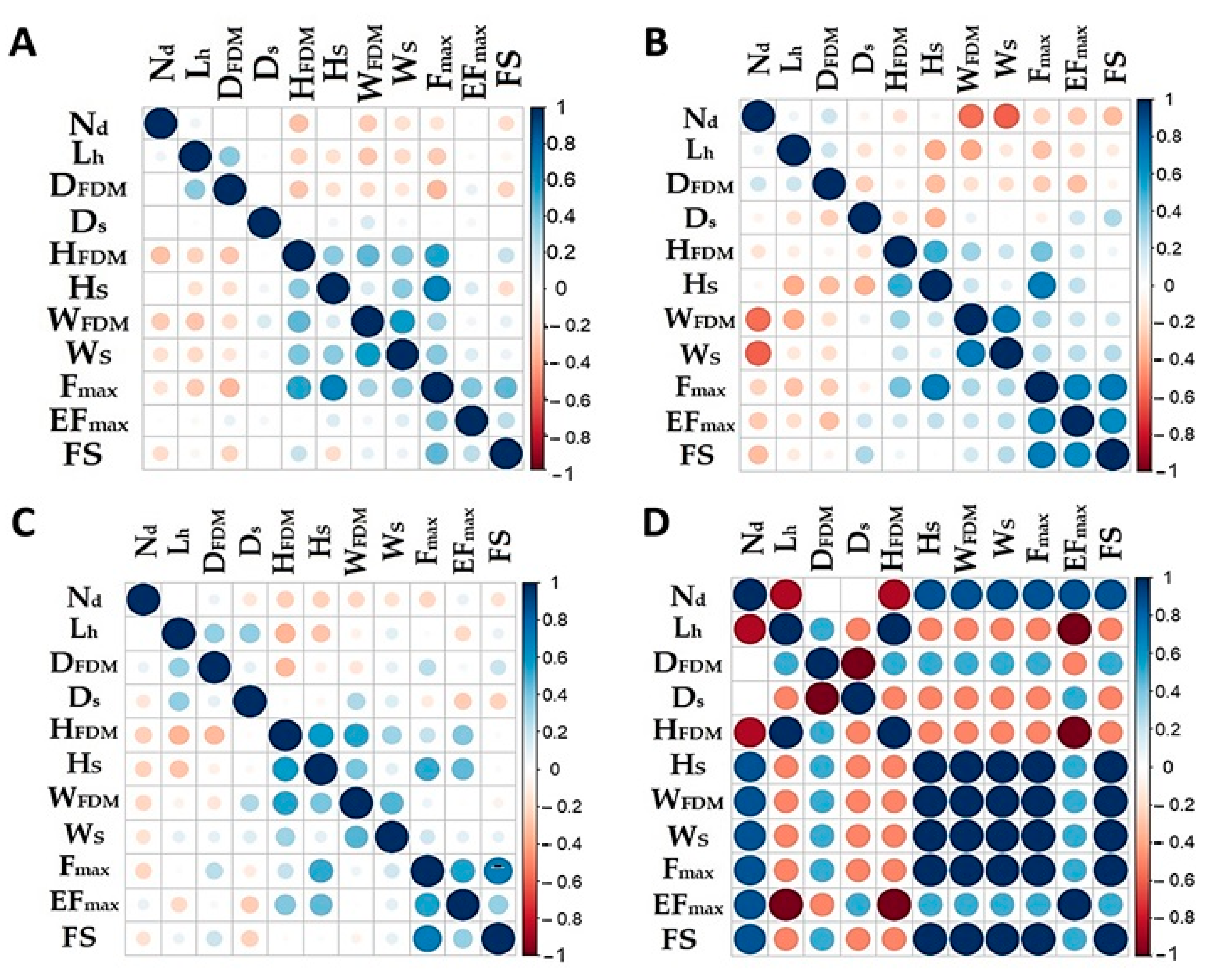
Figure 12.
Spearman correlation between the studied parameters. (A) Group 1; (B) group 2; (C) group 3; and (D) group 4. The interpretation of the abbreviations is provided in the Abbreviations list.
Figure 12.
Spearman correlation between the studied parameters. (A) Group 1; (B) group 2; (C) group 3; and (D) group 4. The interpretation of the abbreviations is provided in the Abbreviations list.
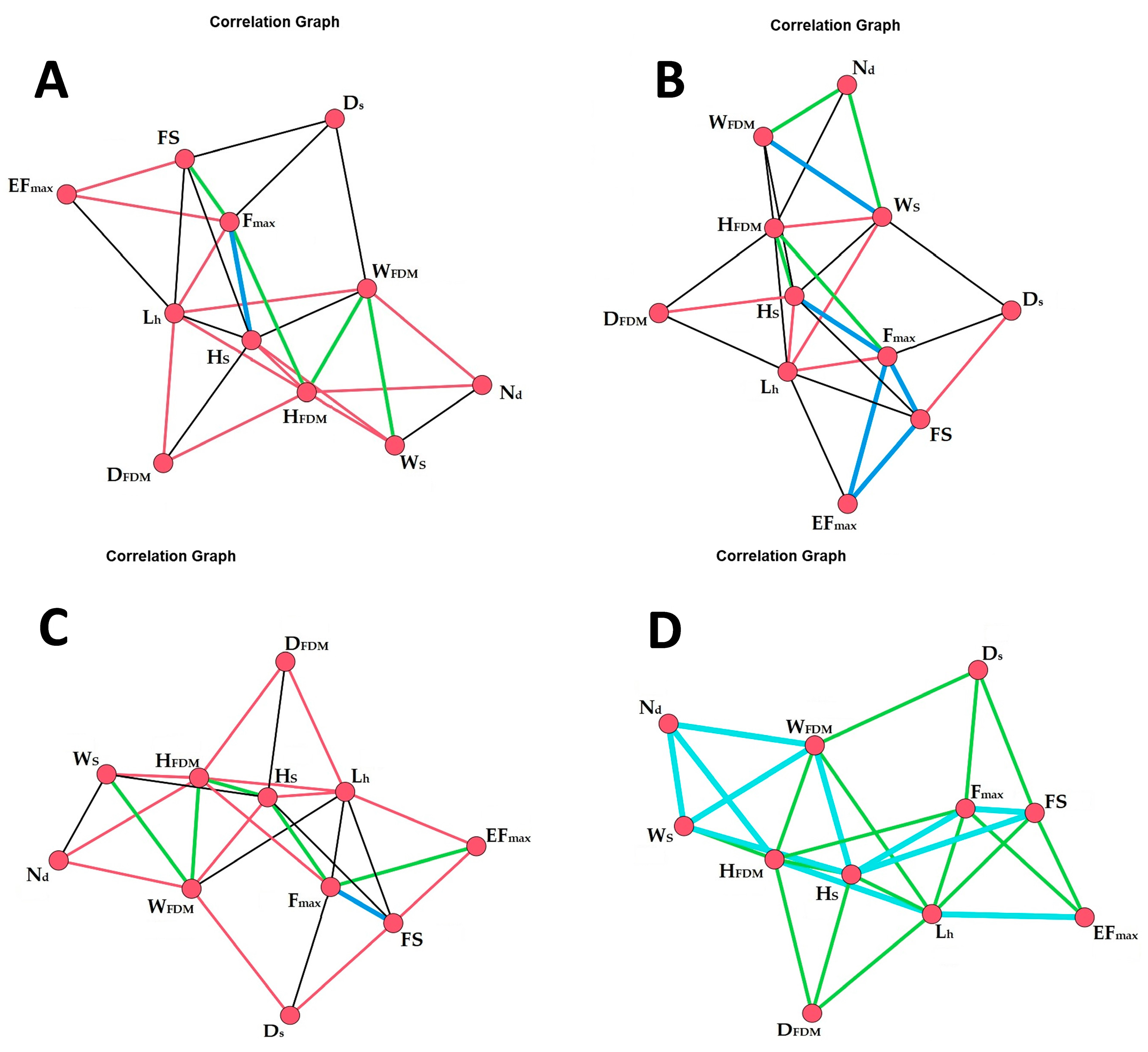
Figure 13.
Graph of the correlation between the analyzed variables for each of the four groups selected by means of hierarchical classification. (A) Sample group 1; (B) sample group 2; (C) sample group 3; and (D) sample group 4. The interpretation of the abbreviations is provided in the Abbreviations list.
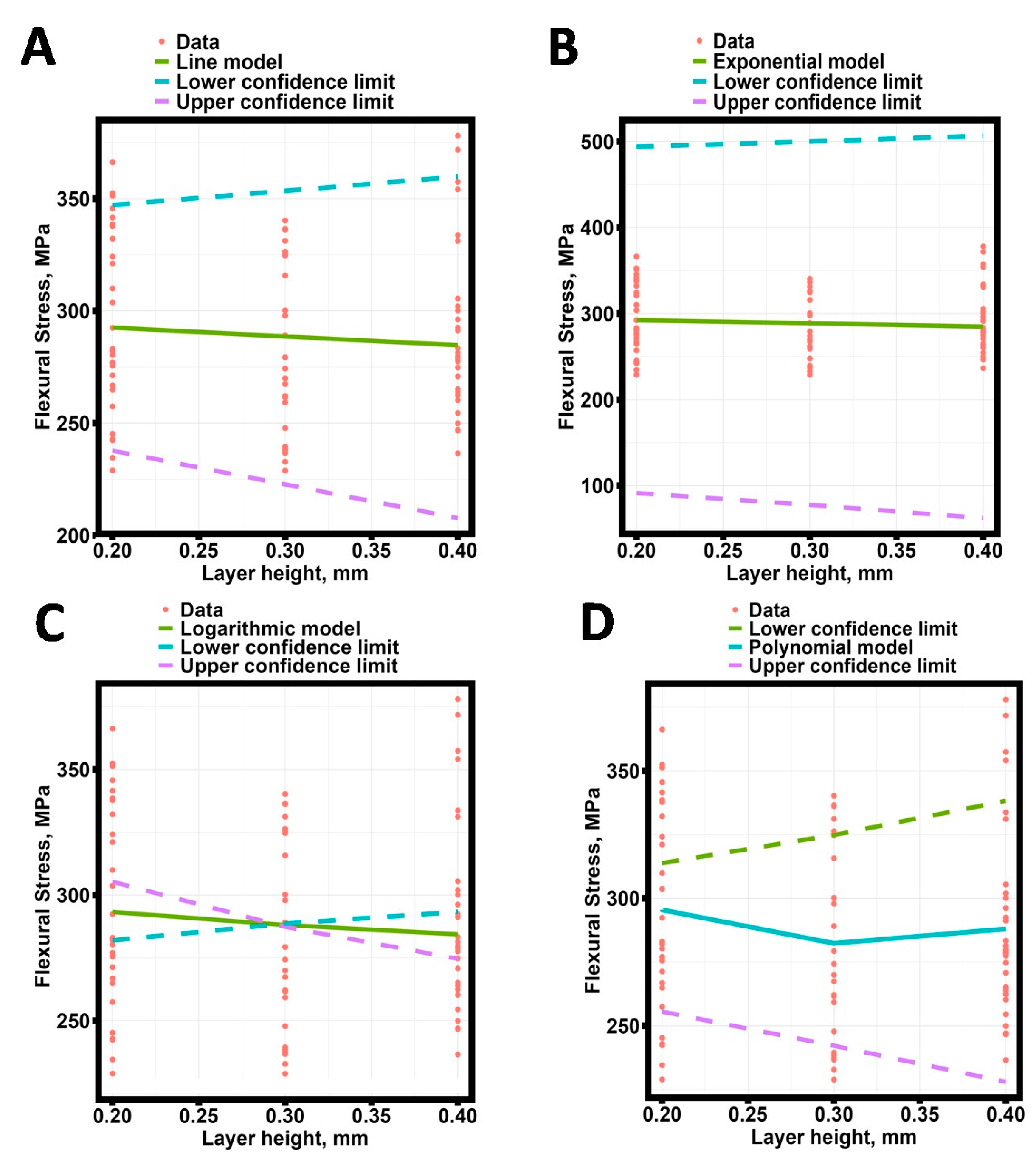
Figure 14.
The dependence of the flexural stress of the zirconium oxide ceramic samples in the biaxial test on the thickness of the filling layer of the workpiece for four robust regression models (first group). (A) Linear model; (B) exponential model; (C) logarithmic model; and (D) polynomial model.
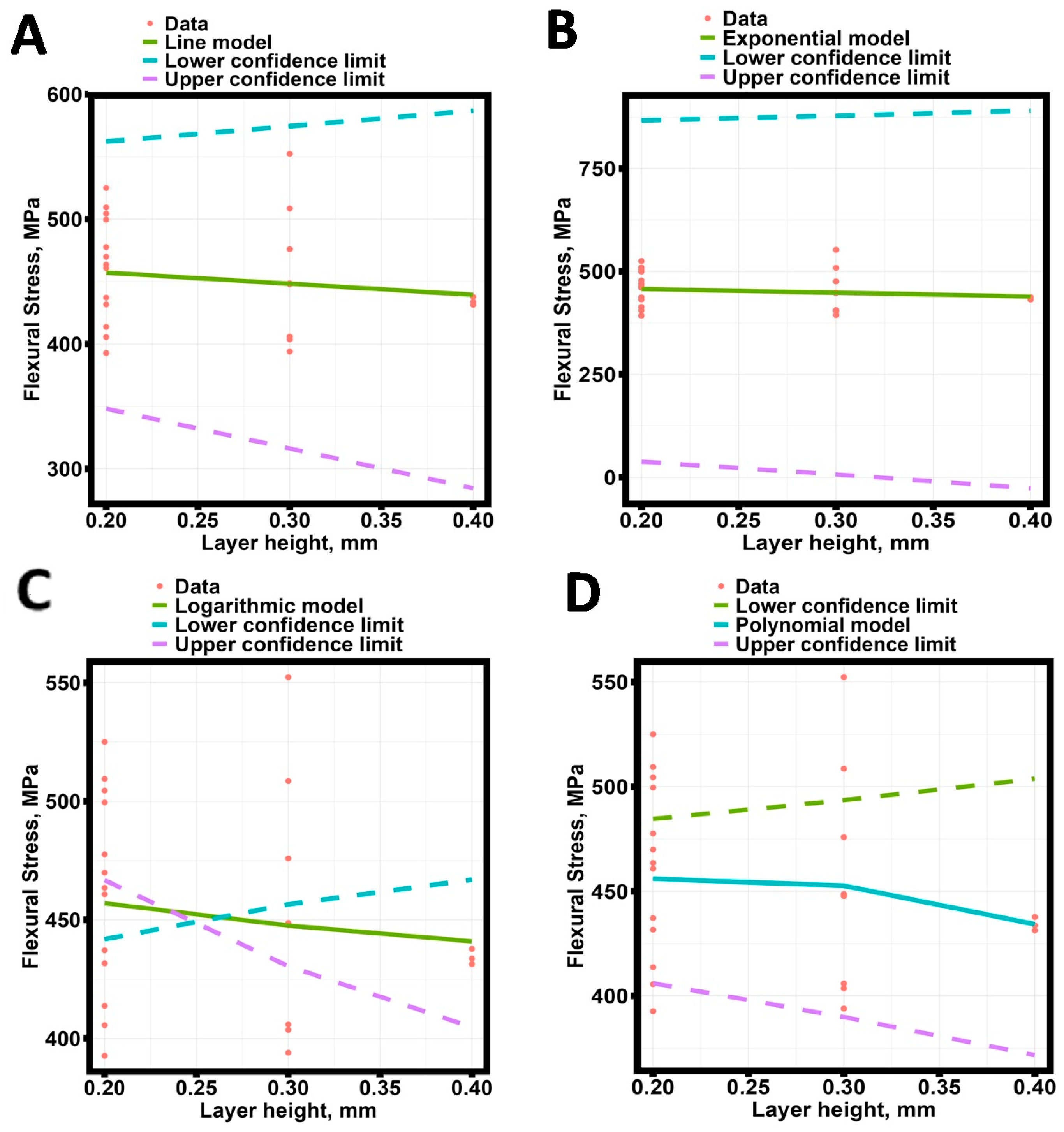
Figure 15.
The dependence of the ultimate stress of the zirconia samples in the biaxial test on the thickness of the filling layer of the workpiece for four robust regression models (second group). (A) Linear model; (B) exponential model; (C) logarithmic model; and (D) polynomial model.
Figure 15.
The dependence of the ultimate stress of the zirconia samples in the biaxial test on the thickness of the filling layer of the workpiece for four robust regression models (second group). (A) Linear model; (B) exponential model; (C) logarithmic model; and (D) polynomial model.
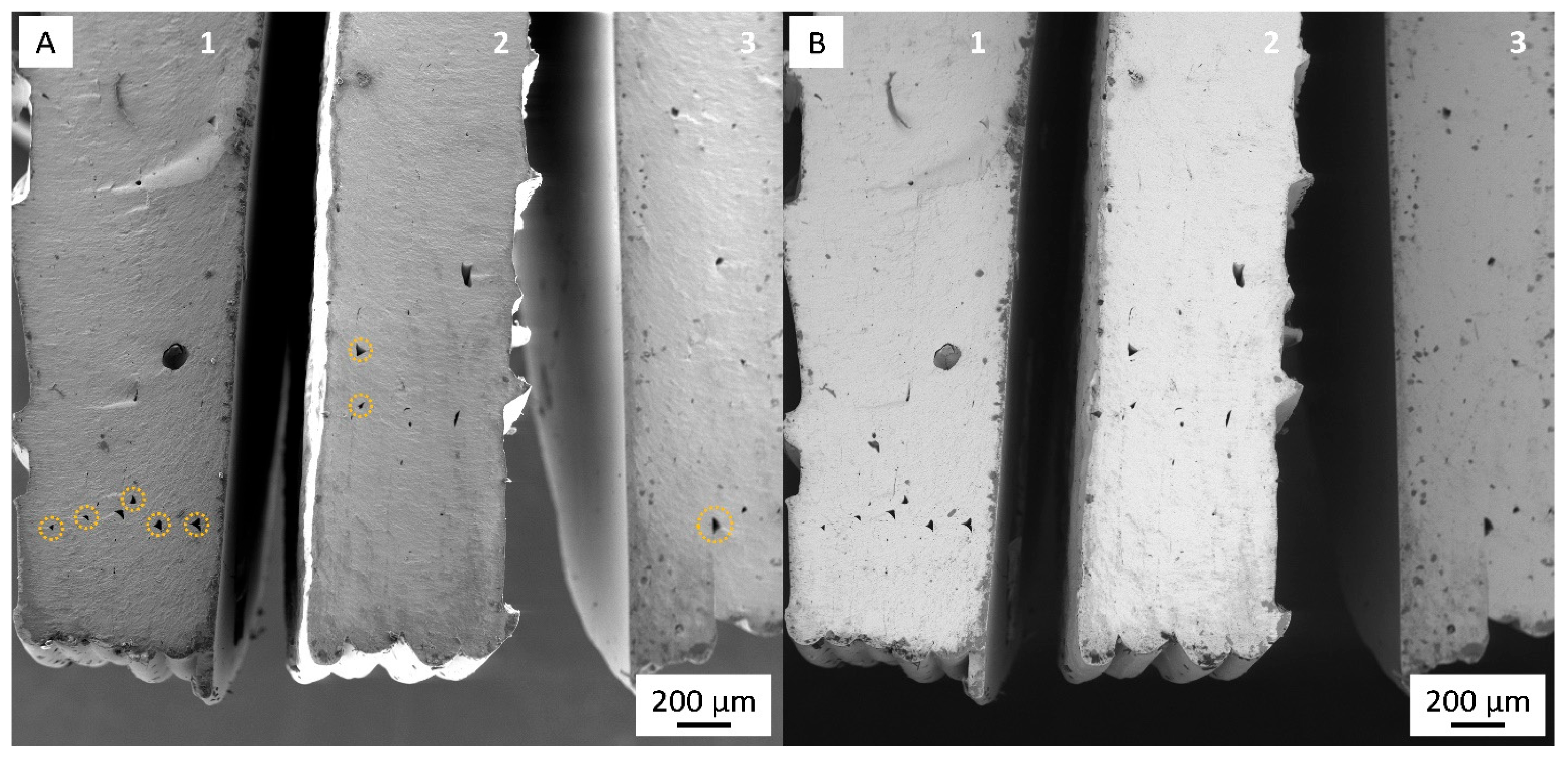
Figure 16.
The SEM micrographs of fractured surfaces in secondary electron (A) and backscattered electron (B) mode. Here, 1, 2, and 3 denote samples in groups 1, 2, and 4, respectively.
Figure 16.
The SEM micrographs of fractured surfaces in secondary electron (A) and backscattered electron (B) mode. Here, 1, 2, and 3 denote samples in groups 1, 2, and 4, respectively.
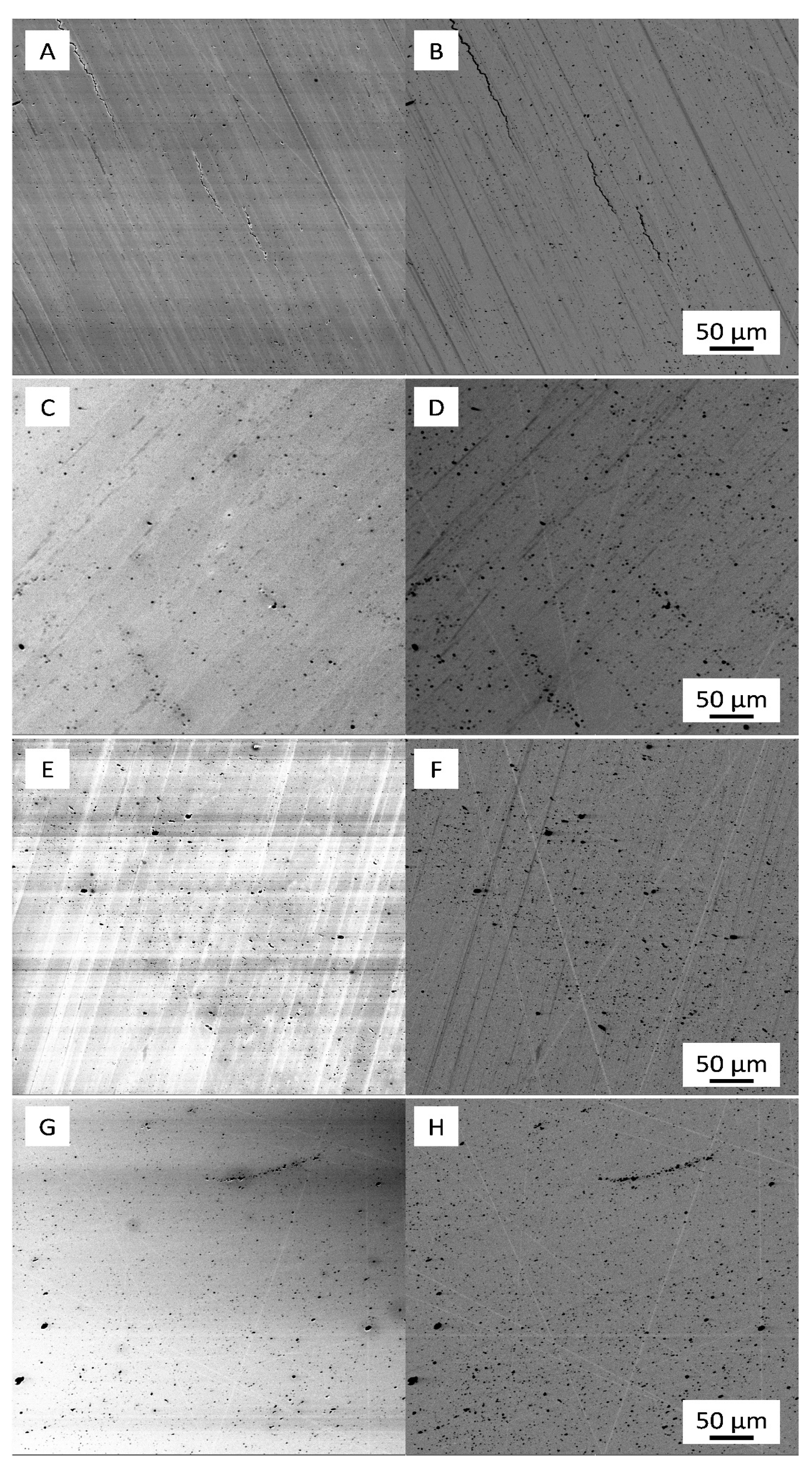
Figure 17.
The SEM images of the magnified fracture surface structure of samples belonging to groups 2 and 4 in secondary electron (left column) and backscattered electron (right column) mode.
Figure 17.
The SEM images of the magnified fracture surface structure of samples belonging to groups 2 and 4 in secondary electron (left column) and backscattered electron (right column) mode.
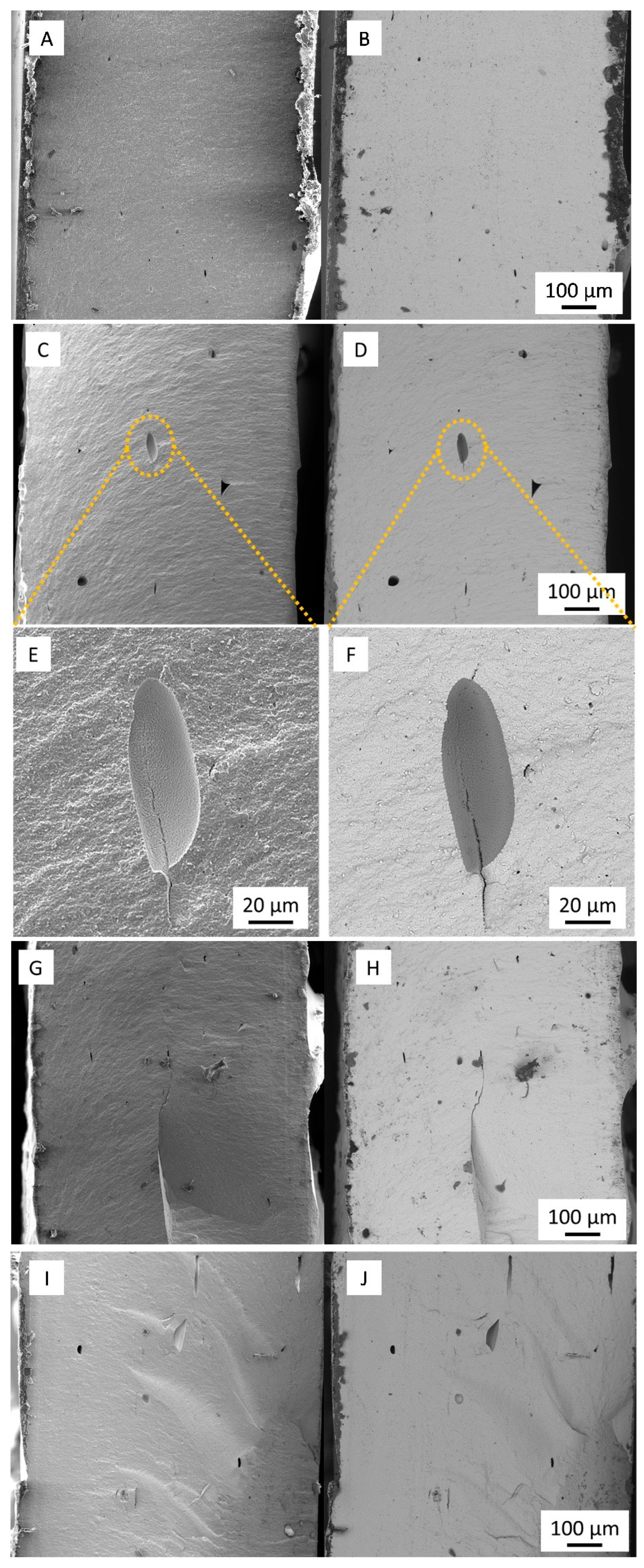
Figure 18.
The SEM image (A,B) of the surface of the zirconium oxide specimen included in the first group. SEM images of the surface of zirconium oxide samples subjected to the biaxial test. (C,D) Sample from 1; (E,F) sample from 2; and (G,H) sample from 3.
Figure 18.
The SEM image (A,B) of the surface of the zirconium oxide specimen included in the first group. SEM images of the surface of zirconium oxide samples subjected to the biaxial test. (C,D) Sample from 1; (E,F) sample from 2; and (G,H) sample from 3.
Figure 19.
Tomographic images of zirconium dioxide ceramic samples tested in the biaxial test. (A,B) Specimen of group 1; (C,D) specimen of group 3; (E,F) and (G,H) specimens of group 2 and 4, respectively.
Figure 19.
Tomographic images of zirconium dioxide ceramic samples tested in the biaxial test. (A,B) Specimen of group 1; (C,D) specimen of group 3; (E,F) and (G,H) specimens of group 2 and 4, respectively.
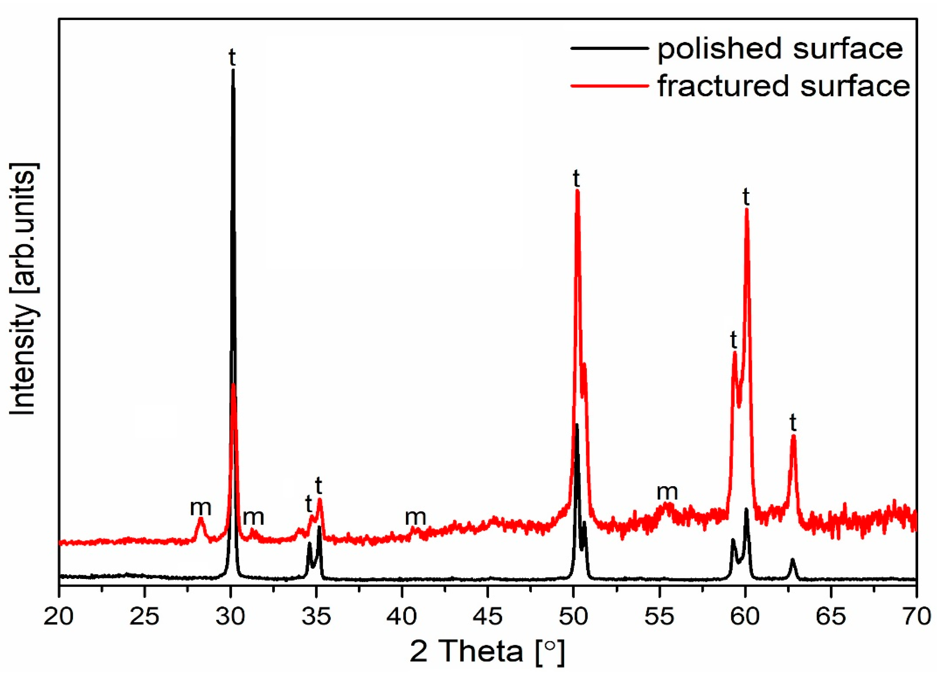
Figure 20.
The XRD analysis of sintered zirconia samples “t” and “m” denote tetragonal and monoclinic phases.
Figure 20.
The XRD analysis of sintered zirconia samples “t” and “m” denote tetragonal and monoclinic phases.
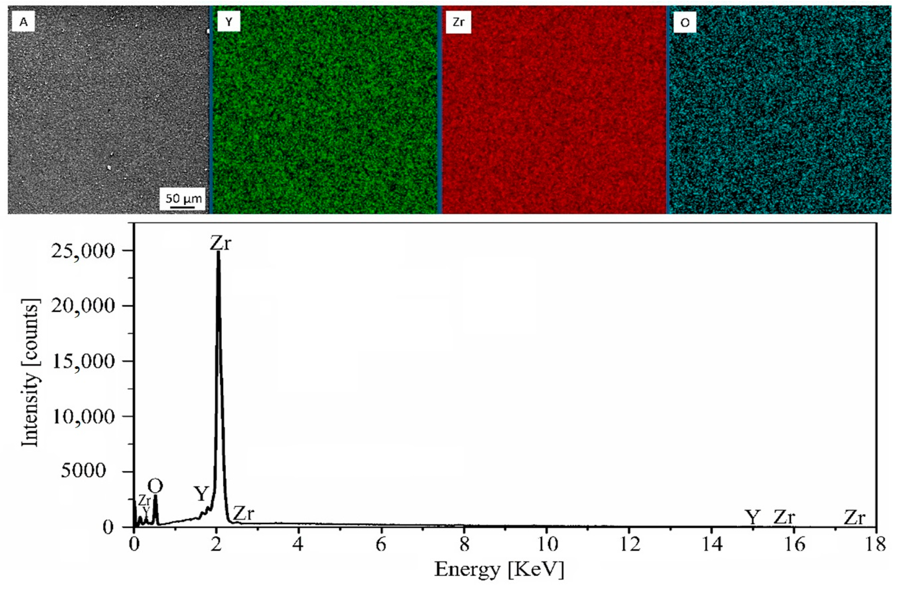
Figure 21.
SEM image (A), EDS distribution maps of yttrium (Y), zirconium (Zr), oxygen (O), and the EDS spectrum of sintered ceramic.
Figure 21.
SEM image (A), EDS distribution maps of yttrium (Y), zirconium (Zr), oxygen (O), and the EDS spectrum of sintered ceramic.
Table 1.
Baseline statistical values of the results of the mechanical tests *.
Table 1.
Baseline statistical values of the results of the mechanical tests *.
| Statistical Value | ND, mm | DFDM, mm | Ds, mm | HFDM, mm | Hs, mm | WFDM, g | Ws,
g | Fmax,
N | EFmax, mm | FS, MPa |
|---|
| Mean value | 0.6 | 24.984 | 19.816 | 1.292 | 1.090 | 1.837 | 1.542 | 211.412 | 0.089 | 309.625 |
| Standard deviation | 0.311 | 0.198 | 0.295 | 0.296 | 0.0988 | 0.094 | 143.202 | 0.040 | 108.422 |
| Median | 25.015 | 19.854 | 1.191 | 0.996 | 1.821 | 1.518 | 161.936 | 0.08 | 285.583 |
| Minimum value | 24.404 | 19.250 | 1.028 | 0.889 | 1.541 | 1.316 | 66.903 | 0.04 | 142.634 |
| Maximum value | 26.624 | 20.120 | 2.109 | 1.932 | 2.088 | 1.790 | 885.289 | 0.229 | 610.367 |
| First quartile | 24.895 | 19.704 | 1.148 | 0.929 | 1.786 | 1.495 | 130.367 | 0.061 | 236.462 |
| Third quartile | 25.107 | 19.969 | 1.278 | 1.045 | 1.865 | 1.576 | 224.757 | 0.109 | 335.545 |
| Mean value | 0.8 | 24.886 | 19.927 | 1.268 | 1.057 | 1.852 | 1.552 | 155.954 | 0.071 | 244.385 |
| Standard deviation | 0.517 | 0.126 | 0.199 | 0.155 | 0.193 | 0.154 | 88.700 | 0.032 | 92.880 |
| Median | 24.775 | 19.935 | 1.253 | 1.045 | 1.847 | 1.545 | 145.334 | 0.064 | 228.909 |
| Minimum value | 23.754 | 19.562 | 1.037 | 0.909 | 1.526 | 1.301 | 56.772 | 0.027 | 106.344 |
| Maximum value | 27.723 | 20.250 | 2.329 | 2.031 | 3.089 | 2.594 | 651.168 | 0.178 | 475.855 |
| First quartile | 24.676 | 19.871 | 1.1575 | 0.975 | 1.797 | 1.514 | 101.309 | 0.048 | 162.037 |
| Third quartile | 25.011 | 19.995 | 1.337 | 1.096 | 1.889 | 1.566 | 183.362 | 0.091 | 302.850 |
| Mean value | 1 | 25.013 | 19.768 | 1.152 | 0.985 | 1.757 | 1.484 | 166.095 | 0.092 | 301.299 |
| Standard deviation | 0.286 | 0.258 | 0.047 | 0.057 | 0.095 | 0.093 | 62.972 | 0.044 | 114.303 |
| Median | 25.052 | 19.802 | 1.147 | 0.986 | 1.765 | 1.498 | 146.226 | 0.086 | 268.356 |
| Minimum value | 24.226 | 19.207 | 1.085 | 0.851 | 1.391 | 1.028 | 55.977 | 0.031 | 115.530 |
| Maximum value | 26.060 | 20.301 | 1.385 | 1.113 | 1.883 | 1.602 | 365.734 | 0.316 | 684.096 |
| First quartile | 24.954 | 19.627 | 1.123 | 0.949 | 1.725 | 1.475 | 125.377 | 0.062 | 237.706 |
| Third quartile | 25.115 | 19.947 | 1.173 | 1.019 | 1.823 | 1.510 | 216.354 | 0.105 | 383.847 |
Table 2.
Baseline statistical values of the results of the flexural tests grouped by the fill layer thickness (H) parameter *.
Table 2.
Baseline statistical values of the results of the flexural tests grouped by the fill layer thickness (H) parameter *.
| Statistical Value | Lh, mm | DFDM, mm | Ds, mm | HFDM, mm | Hs, mm | WFDM,
g | Ws,
g | Fmax,
N | EFmax,
mm | FS,
MPa |
|---|
| Mean value | 0.2 | 24.865 | 19.834 | 1.332 | 1.128 | 1.858 | 1.556 | 230.198 | 0.097 | 314.318 |
| Standard deviation | 0.346 | 0.178 | 0.319 | 0.312 | 0.195 | 0.165 | 152.946 | 0.050 | 115.904 |
| Median | 24.890 | 19.907 | 1.215 | 1.018 | 1.832 | 1.514 | 182.610 | 0.086 | 287.691 |
| Minimum value | 24.336 | 19.25 | 1.098 | 0.851 | 1.526 | 1.301 | 66.903 | 0.032 | 106.344 |
| Maximum value | 26.624 | 20.083 | 2.329 | 2.031 | 3.089 | 2.594 | 885.289 | 0.316 | 684.096 |
| First quartile | 24.634 | 19.719 | 1.154 | 0.979 | 1.779 | 1.498 | 142.727 | 0.064 | 236.461 |
| Third quartile | 25.071 | 19.960 | 1.301 | 1.074 | 1.883 | 1.552 | 248.985 | 0.113 | 386.046 |
| Mean value | 0.3 | 24.966 | 19.816 | 1.185 | 1.006 | 1.797 | 1.508 | 155.724 | 0.078 | 275.248 |
| Standard deviation | 0.454 | 0.173 | 0.088 | 0.070 | 0.117 | 0.106 | 61.812 | 0.031 | 114.126 |
| Median | 24.967 | 19.842 | 1.160 | 1.010 | 1.823 | 1.529 | 142.661 | 0.071 | 261.569 |
| Minimum value | 24.226 | 19.344 | 1.028 | 0.886 | 1.3913 | 1.028 | 56.772 | 0.029 | 115.584 |
| Maximum value | 27.723 | 20.129 | 1.385 | 1.124 | 1.982 | 1.688 | 310.520 | 0.174 | 591.013 |
| First quartile | 24.772 | 19.720 | 1.131 | 0.944 | 1.763 | 1.491 | 111.105 | 0.055 | 189.251 |
| Third quartile | 25.086 | 19.942 | 1.250 | 1.054 | 1.861 | 1.569 | 188.934 | 0.093 | 328.750 |
| Mean value | 0.4 | 25.056 | 19.865 | 1.196 | 0.997 | 1.794 | 1.516 | 145.384 | 0.075 | 262.894 |
| Standard deviation | 0.344 | 0.264 | 0.125 | 0.081 | 0.072 | 0.057 | 47.865 | 0.030 | 88.724 |
| Median | 25.071 | 19.914 | 1.174 | 0.987 | 1.805 | 1.510 | 142.395 | 0.069 | 261.329 |
| Minimum value | 23.754 | 19.207 | 1.048 | 0.889 | 1.603 | 1.372 | 55.977 | 0.027 | 115.53 |
| Maximum value | 26.060 | 20.301 | 1.640 | 1.248 | 1.964 | 1.621 | 286.919 | 0.178 | 610.367 |
| First quartile | 24.962 | 19.764 | 1.119 | 0.935 | 1.741 | 1.487 | 112.454 | 0.056 | 195.486 |
| Third quartile | 25.203 | 20.061 | 1.201 | 1.022 | 1.844 | 1.564 | 169.968 | 0.096 | 295.246 |
Table 3.
Baseline statistical values of the results of the mechanical test results, grouped by the infill pattern *.
Table 3.
Baseline statistical values of the results of the mechanical test results, grouped by the infill pattern *.
| Statistical Value | Infill Pattern | DFDM, mm | Ds, mm | HFDM, mm | Hs, mm | WFDM, g | Ws, g | Fmax, N | EFmax, mm | FS, MPa |
|---|
| Mean value | ZigZag | 24.811 | 19.864 | 1.173 | 1.004 | 1.770 | 1.493 | 154.317 | 0.0724 | 278.568 |
| Standard deviation | 0.304 | 0.201 | 0.083 | 0.067 | 0.121 | 0.107 | 67.127 | 0.030 | 124.144 |
| Median | 24.851 | 19.897 | 1.175 | 0.994 | 1.793 | 1.514 | 144.254 | 0.069 | 263.479 |
| Minimum value | 23.754 | 19.267 | 1.037 | 0.900 | 1.391 | 1.028 | 56.772 | 0.027 | 106.344 |
| Maximum value | 25.388 | 20.130 | 1.385 | 1.177 | 1.995 | 1.688 | 310.520 | 0.136 | 610.367 |
| First quartile | 24.664 | 19.787 | 1.106 | 0.954 | 1.738 | 1.484 | 105.942 | 0.049 | 186.866 |
| Third quartile | 25.033 | 19.988 | 1.2403 | 1.035 | 1.835 | 1.554 | 197.121 | 0.094 | 334.310 |
| Mean value | Concentric | 25.043 | 19.808 | 1.304 | 1.096 | 1.821 | 1.528 | 203.715 | 0.096 | 289.917 |
| Standard deviation | 0.481 | 0.197 | 0.297 | 0.288 | 0.108 | 0.094 | 137.845 | 0.049 | 84.372 |
| Median | 25.0095 | 19.774 | 1.178 | 0.994 | 1.816 | 1.50105 | 169.909 | 0.085 | 276.963 |
| Minimum value | 24.436 | 19.250 | 1.028 | 0.851 | 1.603 | 1.301 | 55.977 | 0.031 | 115.530 |
| Maximum value | 27.723 | 20.301 | 2.109 | 1.932 | 2.088 | 1.79 | 885.289 | 0.316 | 591.013 |
| First quartile | 24.823 | 19.673 | 1.144 | 0.931 | 1.764 | 1.484 | 136.825 | 0.067 | 239.381 |
| Third quartile | 25.097 | 19.964 | 1.279 | 1.093 | 1.866 | 1.568 | 195.574 | 0.106 | 331.893 |
| Mean value | Linear | 24.997 | 19.852 | 1.230 | 1.027 | 1.856 | 1.558 | 171.822 | 0.080 | 285.250 |
| Standard deviation | 0.291 | 0.229 | 0.175 | 0.152 | 0.180 | 0.149 | 92.593 | 0.031 | 120.352 |
| Median | 25.050 | 19.918 | 1.189 | 1.003 | 1.836 | 1.542 | 143.127 | 0.069 | 260.233 |
| Minimum value | 24.343 | 19.207 | 1.089 | 0.886 | 1.716 | 1.470 | 71.489 | 0.038 | 115.584 |
| Maximum value | 26.060 | 20.250 | 2.329 | 2.031 | 3.089 | 2.594 | 651.168 | 0.174 | 684.096 |
| First quartile | 24.910 | 19.804 | 1.148 | 0.979 | 1.797 | 1.510 | 113.473 | 0.057 | 195.646 |
| Third quartile | 25.142 | 19.987 | 1.305 | 1.046 | 1.872 | 1.565 | 205.697 | 0.099 | 345.652 |
Table 4.
The evaluation of the closest theoretical type of the flexural stress distribution of the zirconium oxide specimens tested.
Table 4.
The evaluation of the closest theoretical type of the flexural stress distribution of the zirconium oxide specimens tested.
| Criterion | Distribution Type |
|---|
| Normal | Lognormal | Logistical | Gamma | Weybull | Exponential | Gumbel | Cauchy |
|---|
| Akaike | 1994.148 | 1969.620 | 1990.064 | 1970.721 | 1986.989 | 2170.777 | 1969.973 | 2029.095 |
| Bayesian | 2000.335 | 1975.807 | 1996.252 | 1976.909 | 1993.177 | 2173.871 | 1976.160 | 2035.283 |
Table 5.
The evaluation of the closest theoretical type of strain distribution corresponding to the maximum force of the zirconium oxide ceramic specimens tested.
Table 5.
The evaluation of the closest theoretical type of strain distribution corresponding to the maximum force of the zirconium oxide ceramic specimens tested.
| Criterion | Distribution Type |
|---|
| Normal | Lognormal | Logistical | Gamma | Weybull | Exponential | Gumbel | Cauchy |
|---|
| Akaike | −585.945 | −651.194 | −614.515 | −641.083 | −611.167 | −479.935 | −647.446 | −584.931 |
| Bayesian | −579.757 | −645.006 | −608.327 | −634.896 | −604.980 | −476.841 | −641.258 | −578.743 |
Table 6.
The results of testing the data for conformity to the normal distribution law using the Kolmogorov–Smirnov test *.
Table 6.
The results of testing the data for conformity to the normal distribution law using the Kolmogorov–Smirnov test *.
| Kolmogorov–Smirnov Statistic | DFDM, mm | Ds, mm | HFDM, mm | Hs, mm | WFDM, g | Ws, g | Fmax, N | ε, mm | σF, MPa |
|---|
| D | 1.000 | 1.000 | 0.848 | 0.803 | 0.928 | 0.891 | 1.000 | 0.511 | 1.000 |
| p-value | <0.000001 | <0.000001 | <0.000001 | <0.000001 | <0.000001 | <0.000001 | <0.000001 | <0.000001 | <0.000001 |
Table 7.
The results of applying the Kruskal–Wallis and Dunn’s criteria to evaluate statistically significant differences in the flexural stress of specimens whose blanks were manufactured using nozzles of different diameters.
Table 7.
The results of applying the Kruskal–Wallis and Dunn’s criteria to evaluate statistically significant differences in the flexural stress of specimens whose blanks were manufactured using nozzles of different diameters.
| Nozzle Diameters | 0.6 (p-Value) | 0.8 (p-Value) |
|---|
| 0.8 (p-value) | 0.001 | — |
| 1 (p-value) | 0.289 | 0.008 |
| Kruskal–Wallis (p-value) | 0.010 |
Table 8.
The results of applying the Kruskal–Wallis criterion and Dunn’s criterion to evaluate statistically significant differences in the flexural stress of specimens whose blanks were manufactured with different layer thicknesses.
Table 8.
The results of applying the Kruskal–Wallis criterion and Dunn’s criterion to evaluate statistically significant differences in the flexural stress of specimens whose blanks were manufactured with different layer thicknesses.
| Layer Height | 0.2 (p-Value) | 0.3 (p-Value) |
|---|
| 0.3 (p-value) | 0.018 | — |
| 0.4 (p-value) | 0.006 | 0.361 |
| Kruskal–Wallis (p-value) | 0.030 |
Table 9.
The results of applying the Kruskal–Wallis criterion and Dunn’s criterion to evaluate statistically significant differences in the flexural stress of specimens whose blanks were manufactured with different types of filling.
Table 9.
The results of applying the Kruskal–Wallis criterion and Dunn’s criterion to evaluate statistically significant differences in the flexural stress of specimens whose blanks were manufactured with different types of filling.
| Filling Type | ZigZag (p-Value) | Concentric (p-Value) |
|---|
| Concentric (p-value) | 0.084 | — |
| Linear (p-value) | 0.312 | 0.186 |
| Kruskal–Wallis (p-value) | 0.370 |
Table 10.
A comparison of the tensile strength of zirconium oxide ceramic specimens subjected to biaxial loading in the groups obtained from the hierarchical classification results.
Table 10.
A comparison of the tensile strength of zirconium oxide ceramic specimens subjected to biaxial loading in the groups obtained from the hierarchical classification results.
| Group Number | 1 (p-Value) | 2 (p-Value) | 3 (p-Value) |
|---|
| 2 (p-value) | 0.000 | — | — |
| 3 (p-value) | 0.000 | 0.000 | — |
| 4 (p-value) | 0.007 | 0.314 | 0.000 |
| Kruskal–Wallis (p-value) | 0 |
Table 11.
The centralization of the graph of statistically significant correlation for the samples belonging to the first group *.
Table 11.
The centralization of the graph of statistically significant correlation for the samples belonging to the first group *.
| Parameters Analyzed | Group 1 |
|---|
| Degree Centrality, Equation (1) | Closeness Centrality, Equation (2) | Betweenness Centrality, Equation (3) |
|---|
| Lh | 7 | 0.769 | 6.744 |
| HFDM | 7 | 0.769 | 6.762 |
| HS | 7 | 0.769 | 5.720 |
| WFDM | 6 | 0.714 | 5.637 |
| Fmax | 6 | 0.714 | 4.018 |
| FS | 5 | 0.625 | 1.917 |
| WS | 4 | 0.588 | 0.476 |
| ND | 3 | 0.526 | 0.000 |
| DFDM | 3 | 0.556 | 0.000 |
| DS | 3 | 0.556 | 0.726 |
| EFmax | 3 | 0.526 | 0.000 |
| Centralization | 0.256 | 0.148 | 0.094 |
Table 12.
A comparison of regression relationships by Akaike’s criterion for the different groups of samples.
Table 12.
A comparison of regression relationships by Akaike’s criterion for the different groups of samples.
| Dependence Type | Group 1 | Group 2 | Group 3 | Group 4 |
|---|
| Linear | 857.785 | 265.939 | 506.130 | 34.179 |
| Exponential | 857.813 | 265.921 | 506.034 | 34.368 |
| Logarithmic | 857.670 | 266.002 | 506.419 | 33.439 |
| Polynomial | 858.388 | 267.736 | 504.587 | −158.421 |
Table 13.
Robust regression equations describing the dependence of the flexural stress on fill layer thickness in the FDM printing of blanks.
Table 13.
Robust regression equations describing the dependence of the flexural stress on fill layer thickness in the FDM printing of blanks.
| Group Number | Robust Regression Equation | Standard Deviation |
|---|
| Group 1 | | 42.96 |
| Group 2 | | 62.79 |
| Group 3 | | 36.75 |
| Group 4 | | 0 |
Table 14.
The average content of the components in the samples of each of the four groups.
Table 14.
The average content of the components in the samples of each of the four groups.
| | Sample
Number | Average Content of Constituents, wt.% 1 |
|---|
| Zr | O | Y |
|---|
| Group 1 | 1 | 62.89 | 29.68 | 7.43 |
| 2 | 63.09 | 30.52 | 6.39 |
| 3 | 62.57 | 30.42 | 7.01 |
| Group 2 | 1 | 63.96 | 30.12 | 5.92 |
| 2 | 62.73 | 30.06 | 7.21 |
| 3 | 62.12 | 30.98 | 6.9 |
| Group 3 | 1 | 63.69 | 29.69 | 6.62 |
| 2 | 62.72 | 30.82 | 6.46 |
| 3 | 62.28 | 29.47 | 8.25 |
| Group 4 | 1 | 63.79 | 29.78 | 6.43 |
| 2 | 63.51 | 29.26 | 7.23 |
| 3 | 62.98 | 30.43 | 6.59 |

 ,
, 

