Abstract
This study proposes an automated, visual–geometric fusion method for measuring pupillary height (PH) and interpupillary distance (PD), aiming to replace manual measurements while balancing accuracy, efficiency, and cost accessibility. To this end, a two-layer Ensemble of Regression Tree (ERT) is used to coarsely localize facial landmarks and the pupil center, which is then refined via direction-aware ray casting and edge-side-stratified RANSAC followed by least-squares fitting; in parallel, an RC-BlendMask instance-segmentation module extracts the lowest rim point of the spectacle lens. Head pose and lens-plane depth are estimated with the Perspective-n-Point (PnP) algorithm to enable pixel-to-millimeter calibration and pose gating, thereby achieving 3D quantification of PH/PD under a single-camera setup. In a comparative study with 30 participants against the Zeiss i.Terminal2, the proposed method achieved mean absolute errors of 1.13 mm (PD), 0.73 mm (PH-L), and 0.89 mm (PH-R); Pearson correlation coefficients were r = 0.944 (PD), 0.964 (PH-L), and 0.916 (PH-R), and Bland–Altman 95% limits of agreement were −2.00 to 2.70 mm (PD), −0.84 to 1.76 mm (PH-L), and −1.85 to 1.79 mm (PH-R). Lens segmentation performance reached a Precision of 97.5% and a Recall of 93.8%, supporting robust PH extraction. Overall, the proposed approach delivers measurement agreement comparable to high-end commercial devices on low-cost hardware, satisfies ANSI Z80.1/ISO 21987 clinical tolerances for decentration and prism error, and is suitable for both in-store dispensing and tele-dispensing scenarios.
1. Introduction
As the global usage of eyewear continues to grow, the demand for comfort and customization is likewise on the rise [1]. During the process of selecting lenses and frames, in addition to measuring refractive errors (e.g., myopia and astigmatism) and dispensing, two geometric parameters are critical: interpupillary distance (PD) and pupillary height (PH) [2]. PD is the horizontal distance between the centers of the left and right pupils, and it is used to align the optical centers of the lenses with the visual axes. PH is defined for each eye as the vertical distance from the pupil center (as seen through the lens) to the lowest point of the corresponding spectacle lens rim; this value determines how the optical center or segment height is positioned within the frame. Accurate PD and PH are required to avoid unwanted prism and to ensure comfortable binocular vision. Misalignment can lead to visual discomfort, blur, dizziness, or asthenopia and may reduce tolerance to prolonged wear [3,4]. In current optical dispensing practice, pupillary height (also called fitting height or segment height) is obtained by capturing a calibrated frontal view of the wearer, locating the pupil center for each eye, and measuring its vertical offset relative to the lower rim of the corresponding spectacle lens or a marked fitting cross. Commercial systems such as the Zeiss i.Terminal2 perform this automatically using calibrated imaging, but the required hardware is expensive and typically used in controlled lighting.
Currently, PD is often measured in optical shops or hospitals using pupillometers or PD rulers. However, the accuracy of these methods depends heavily on the operator’s skill, making it prone to errors that may result in prism effects [5]. Although advanced digital positioning devices, such as Zeiss’s i.Terminal2, utilize 3D facial recognition to improve measurement accuracy, their high cost has limited their widespread adoption [6]. To address this challenge, this paper proposes an intelligent pupil height and distance measurement system based on deep learning. The system captures frontal facial images using a camera, employs an ensemble regression tree (ERT) in tandem with the improved instance segmentation algorithm RC-BlendMask for pupil center localization and then computes the three-dimensional coordinates needed to output PD and PH automatically from a single captured frontal image. On our workstation, the full pipeline runs in under one second per frame. The system captures a single frontal image of the wearer, automatically localizes facial landmarks and the pupil centers, segments the spectacle lens rims, and then computes pupillary distance (PD) and pupillary height (PH) without manual ruler alignment. This reduces dependence on operator skill and minimizes manual measurement steps. Because the pipeline runs in under one second per frame on a consumer-grade camera/computer setup and does not rely on specialized multi-camera hardware such as the i.Terminal2, it is suitable for low-cost deployment in routine dispensing. Quantitatively, the mean absolute differences versus i.Terminal2 were 1.13 mm (PD), 0.73 mm (PH-L), and 0.89 mm (PH-R), which fall within commonly cited clinical tolerances for centration and prism (ANSI Z80.1/ISO 21987). These results indicate that clinically acceptable PH/PD measurements can be obtained with commodity hardware and minimal manual intervention.
The evolution of PD and PH measurement methods has undergone several stages. Early approaches relied on straightforward manual tools like PD rulers, which, although simple to operate, were vulnerable to issues such as parallax error—especially when dealing with eye position abnormalities (e.g., strabismus) [7]. To improve accuracy, Xu Guangdi introduced a line-of-sight distance measurement method, which measures along the patient’s actual visual axis rather than relying on external facial landmarks, thereby reducing parallax-related error in cases such as strabismus [8]. The maturation of optical and electronic measurement technologies led to more sophisticated instruments such as handheld pupilometers (e.g., HRK-7000A, Topcon PD-8, Nidek PD Meter II) [9]. Zeiss’s i.Terminal2 system further advanced measurement precision by combining high-resolution cameras and advanced image processing, though it remains cost-prohibitive for broader adoption in many optical shops.
With rapid developments in the internet and computer vision, researchers have explored measuring PD and PH via software applications that utilize image processing and machine learning. For instance, Zheng et al. [10] designed a mobile application that employs an OpenCV-built classifier to locate facial features and calculate PD by comparing pupil positions against a reference object. Other studies have similarly leveraged machine learning to improve pupil detection accuracy, indicating a growing trend toward data-driven methods [11]. Traditional image processing techniques—such as those from Kumar et al. [12] and Gu et al. [13]—often rely on color features, thresholding, and contour tracking to locate the pupil. Although these methods can achieve high-speed detection in certain conditions, they are susceptible to noise, variations in lighting, and occlusion by eyelids, which may reduce accuracy or robustness. More recent works employing convolutional neural networks (CNNs), such as those by Lin et al. [14], Li et al. [15], and Sun et al. [16], demonstrate improved precision and robustness in non-ideal settings. More recently, several studies have begun to fuse low-cost imaging, deep neural inference, and explicit 3D head/eye geometry to achieve fully contactless ocular and facial biometry. Barry and Wang showed that pupil size can be robustly quantified from standard RGB smartphone cameras across different skin tones and iris contrasts by learning a far-red–guided pupil segmentation and calibration pipeline, indicating that accurate pupillometry does not strictly require dedicated ophthalmic hardware [17] Shen et al. combined per-eye keypoint detection with a time-of-flight depth camera and a geometric head–eye model to recover 3D gaze direction in real time, illustrating how learning-based feature localization and 3D reconstruction can be integrated for biometric gaze estimation [18] Ben Barak-Dror et al. used short-wave infrared imaging together with learned pupil/eyelid modeling to perform rapid, contactless pupillometry and gaze estimation even with closed eyelids, highlighting clinical potential in non-cooperative or critical-care scenarios [19]. Qammaz and Argyros presented an occlusion-tolerant pipeline that regresses 3D head pose and gaze direction from a single RGB view using a lightweight deep model, targeting real-time performance without multi-camera rigs [20,21,22]. These recent works reinforce the trend toward low-cost, vision-based, calibration-aware ocular measurements, and motivate our goal: a single-camera system that estimates pupillary distance (PD) and pupillary height (PH) with accuracy comparable to specialized commercial devices while satisfying clinical tolerances. Recent work in facial landmark localization has moved beyond classical cascaded regressors, using dense 3D face modeling for large-pose alignment (e.g., 3DDFA) [23], multi-stage CNN refinement with global facial context (e.g., Deep Alignment Network) [24], and loss functions such as Wing and Adaptive Wing loss that emphasize small localization errors to improve robustness under occlusion and pose variation [25]. High-capacity boundary-aware and stacked-hourglass architectures have pushed performance on both 2D and 3D alignment benchmarks, especially under challenging illumination and expression conditions [26]. These advances form the technical background of our work: we target the same need for reliable ocular landmarks under real-world head pose and eyelid occlusion, but with a lightweight two-layer regression-tree cascade rather than a heavy multi-stage heatmap network so that the system can run on a single consumer camera in a retail dispensing setting [27].
Building on prior work in computer vision–based optical measurement, this study makes the following contributions:
- (1)
- Automated PD/PH measurement from a single RGB image.
We develop an end-to-end system that captures a single frontal image of the wearer, localizes facial landmarks, estimates the pupil centers, segments the spectacle lenses, and computes interpupillary distance (PD) and pupillary height (PH) in physical units. The workflow is shown in Figure 1. The system is designed to run on commodity hardware without multi-camera rigs.
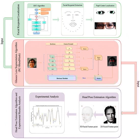
Figure 1.
Research technical route illustrating the overall methodology of the study, including data acquisition, preprocessing, model training, and evaluation stages. Consent has been sought from the parties to place the photos to avoid unnecessary copyright.
- (2)
- Two-layer ERT landmarking with pupil-center refinement.
We train a two-layer Ensemble of Regression Trees (ERT) for facial keypoint localization and coarse pupil-center seeding. We then refine the pupil centers using direction-aware ray casting, edge-side–stratified RANSAC, and final least-squares circle fitting. This reduces sensitivity to eyelid occlusion and improves localization stability under non-ideal gaze/illumination.
- (3)
- Spectacle lens segmentation via RC-BlendMask.
We introduce RC-BlendMask, an enhanced instance-segmentation model that fuses BlendMask with RCF-style edge features to suppress boundary diffusion and recover clean lens rims. Precise spectacle lens rim segmentation is required to identify the lowest point on each lens, which is used in the definition of pupillary height (PH is the vertical distance from the pupil center to the lowest point of the corresponding spectacle lens rim). Without reliable rim extraction, PH cannot be computed consistently.
- (4)
- Head-pose gating and 3D pixel-to-mm calibration.
We estimate head pose with a PnP-based solver from 2D facial landmarks, recover Euler angles (yaw/pitch/roll), and reject frames whose pose exceeds predefined thresholds. We also use the recovered pose and camera intrinsics to perform pixel–millimeter conversion on the lens plane, enabling 3D-aware PD/PH estimation from a monocular camera.
- (5)
- Quantitative robustness and agreement analysis.
We evaluate the system on 30 participants against a commercial device (Zeiss i.Terminal2). Robustness is quantified using multiple statistical measures: mean absolute error (MAE) and root-mean-squared error (RMSE), Pearson correlation, Bland–Altman bias and 95% limits of agreement (LOA), and repeatability metrics (within-subject SD, repeatability coefficient). The mean absolute differences versus i.Terminal2 were 1.13 mm for PD, 0.73 mm for left PH, and 0.89 mm for right PH, all within commonly cited ANSI Z80.1/ISO 21987 tolerances on decentration and unwanted prism. We also report segmentation quality (Precision, Recall, F1, IoU) for RC-BlendMask and head-pose MAE (yaw/pitch/roll) on public pose datasets.
- (6)
- Practical deployment perspective.
Because our pipeline uses a single off-the-shelf camera and standard compute, rather than proprietary multi-camera hardware, it has the potential to lower measurement cost while maintaining clinically acceptable agreement with an established commercial reference.
Recent work in optical metrology and computational optics has shown that deep learning can augment physically motivated imaging pipelines, for example by suppressing stray light in wide-field astronomical imaging or learning to emulate ghost reflections in optical systems [17,18]. Our results extend this vision–geometry fusion trend to ophthalmic dispensing, targeting contactless PH/PD measurement suitable for routine retail and tele-optometry use.
This paper is structured as follows: Section 2 details the materials and methods employed, including the ensemble regression trees for facial keypoint localization, the RC-BlendMask algorithm for lens segmentation, and the PNP-based head pose estimation technique. Section 3 presents experimental results and discussion, showcasing comparative analyses against the Zeiss i.Terminal2 device, evaluating error sources, and demonstrating the system’s robustness. Finally, Section 4 concludes by summarizing the primary findings, highlighting the system’s practical relevance, and discussing potential avenues for further refinement of both the algorithms and the overall measurement strategy.
2. Materials and Methods
2.1. System Pipeline and Facial Keypoint Localization (ERT)
As shown in Figure 2, the end-to-end pipeline consists of frontal face acquisition, initial pupil and facial landmark localization using an ERT model, PnP-based head pose evaluation and pose-based rejection, refinement of pupil centers via direction-constrained ray casting and edge-stratified RANSAC, RC-BlendMask-based lens contour extraction and lowest rim point detection, and finally metric conversion using camera intrinsics and lens plane depth to output interpupillary distance (PD) and pupillary height (PH) in millimeters.
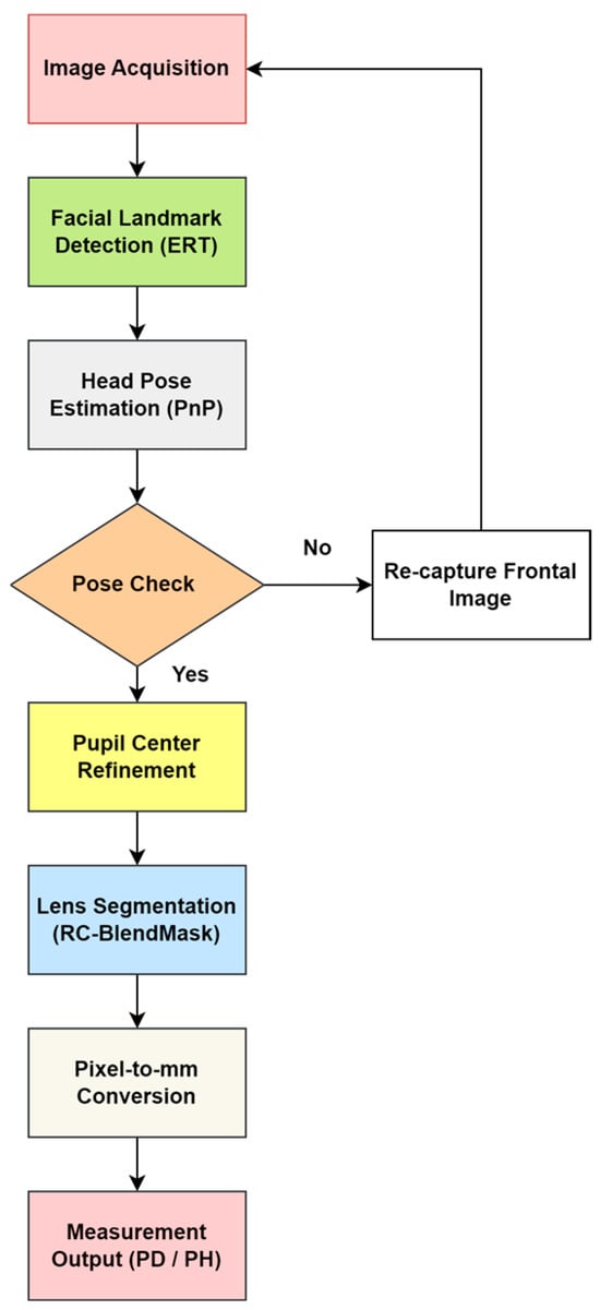
Figure 2.
Overall workflow of the proposed automatic measurement system.
This subsection gives a high-level overview of the full pipeline. The detailed algorithms and parameter settings are described in Section 2.1.1, Section 2.1.2, Section 2.1.3, Section 2.1.4, Section 2.1.5, Section 2.2, Section 2.3, Section 2.4. The workflow (Figure 2) is as follows.
- (1)
- A frontal facial image is captured while the subject is wearing spectacles.
- (2)
- The system detects facial keypoints and segments the spectacle lens region (facial keypoint localization, Section 2.1.1 and Section 2.1.2; lens segmentation with RC-BlendMask, Section 2.3.
- (3)
- The system estimates head pose and extracts the Euler angles. If the angles fall within predefined thresholds, the image is accepted; if not, the subject is asked to provide a new frontal image (head-pose estimation, Section 2.4.
- (4)
- The pupil centers are then localized using the improved pupil-center module (Section 2.3).
- (5)
- The three-dimensional coordinates of each pupil center and the lowest point of each lens rim are computed.
- (6)
- Finally, the system automatically computes interpupillary distance (PD, the distance between the left and right pupil centers) and pupillary height (PH, the vertical distance from each pupil center to the lowest point of the corresponding spectacle lens rim) and reports the results. (measurement algorithm, Section 2.4).
In summary, the deep learning–based measurement program operates in a loop: capture a frontal face image, detect facial landmarks, segment the lenses, check head pose, and only proceed if the pose is acceptable. After that, it refines the pupil center locations, recovers the 3D coordinates of the pupil centers and the lowest lens points, and automatically outputs PD and PH. The technical roadmap is shown in Figure 3.
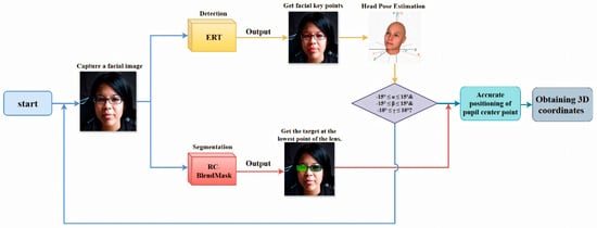
Figure 3.
Intelligent detection procedure flowchart showing the sequential steps from image input, facial detection, and keypoint extraction, to measurement calculation and results output. Consent has been sought from the parties to place the photos to avoid unnecessary copyright issues.
2.1.1. Facial Key Point Localization
In this work, “facial keypoints” are 2D anatomical landmarks on the face, including the inner and outer eye corners, eyelid margins, nose tip, mouth corners, and jawline contour. We follow standard 68-point (300W) and 98-point (WFLW) landmark definitions, in which each face is annotated with a consistent set of reference locations for both eyes, the nose, the mouth, and the facial outline (see Figure 4). These coordinates are used in our pipeline to (i) crop and normalize the eye region, (ii) obtain an initial estimate of the pupil center, and (iii) provide 2D–3D correspondences for Perspective-n-Point (PnP) head pose estimation. Accurate keypoint localization is therefore essential for reliable PD and PH measurement.
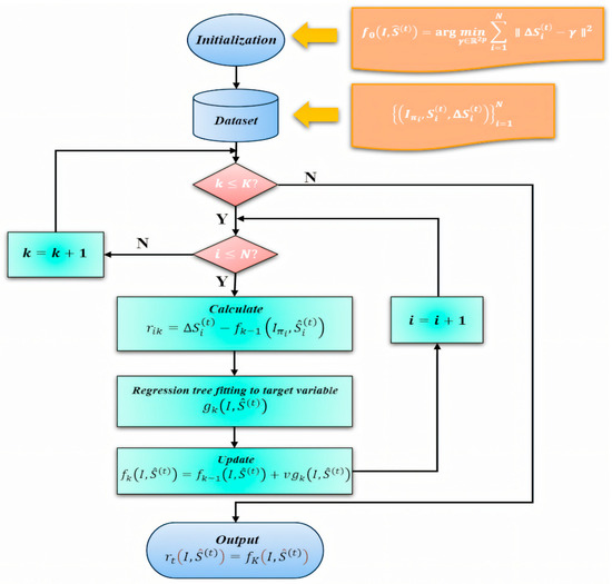
Figure 4.
Training workflow of the ERT-based facial landmark module. The diagram illustrates data preprocessing and initialization, computation of residuals , regression tree fitting under a gradient-boosting framework, the model update with learning rate , and validation. Note that this figure describes the ERT module only; other components (e.g., RC-BlendMask for lens segmentation and PnP-based head-pose estimation) are trained separately.
We adopt an Ensemble of Regression Trees (ERT)–based landmark regressor that predicts facial keypoints directly from image intensities. Building on the classical ERT framework of Kazemi and Sullivan [28], we train a two-layer regression cascade and fine-tune its key parameters with special emphasis on the periocular region. The first layer provides a coarse but stable initialization of the global facial shape. The second layer refines local structure around the eyes to improve pupil seeding and downstream head-pose estimation. This two-layer strategy improves generalization under variations in lighting, facial expression, and moderate head pose, and increases eye-region precision, which is critical for subsequent pupil-center localization.
In our implementation, each stage of the cascade incrementally corrects the current landmark estimate, and the regressor is optimized to minimize squared error. We also adjust shrinkage, tree depth, and oversampling of perturbed initial shapes to balance accuracy and robustness for real-time use.
2.1.2. ERT Algorithm
The ERT algorithm provides high-precision and robust facial keypoint localization. It performs reliably even under challenging conditions such as changes in lighting, facial expression, and head pose. It is also easy to tune, and it can tolerate missing labels in the training data, which makes it suitable for large-scale and real-time applications.
In this study, we train an ensemble of regression trees using a gradient boosting framework that minimizes the sum of squared error. To further improve performance, we introduce a two-layer regression structure. The first layer provides a stable coarse estimate, and the second layer refines it. This hierarchical design improves generalization and makes the model more adaptable and efficient in difficult cases.
In the first stage of training, the algorithm utilizes a dataset , where represents the input images, and corresponds to the coordinates of the facial key points. A cascading regression scheme is employed, in which each regressor builds upon the predictions of its predecessors. Specifically, the updated key point predictions at iteration t + 1 are given by (1). where represents the regressor at the t-th iteration. The difference between the true key points and the predicted values is expressed as (2).
This cascading approach organizes the dataset into triplets , enabling the iterative training of a sequence of regression models , which progressively refine the predictions.
The second stage of the model involves training each regression function using a gradient boosting tree algorithm. The loss function is formulated as (3).
where the term represents the gradient. To prevent overfitting and improve the model’s stability, a learning parameter (with ) is introduced. This process facilitates the optimization of the regression functions within the cascade, as illustrated by the diagram depicting the training progression for each .
This process facilitates the optimization of the regression functions within the cascade. Figure 4 summarizes the training workflow of the ERT-based facial landmark module (rather than the entire pipeline), including residual computation , regression-tree fitting within the gradient-boosting scheme, and the learning-rate–controlled update , followed by validation.
By integrating these two layers of regression, the proposed approach enhances the model’s precision and adaptability, enabling it to address the complexities inherent in facial key point localization tasks.
2.1.3. Dataset Collection and Preprocessing
The 300W dataset is a widely adopted benchmark for 68-point facial landmark alignment. It unifies images from LFPW, AFW, HELEN, XM2VTS, and IBUG under a single annotation protocol and comprises 3148 training and 689 test images [29]. Standard evaluation typically reports results on the Common, Challenging, and Full subsets using normalized mean error (NME, normalized by inter-ocular distance, IOD), the area under the cumulative error distribution at 0.08 (AUC@0.08), and failure rate at NME > 0.10. By contrast, WFLW contains 10,000 in-the-wild images annotated with 98 landmarks and is explicitly curated to probe robustness under difficult conditions such as large pose, occlusion, expression, illumination, and blur; attribute-specific test splits are provided and the dataset has become a standard reference in recent studies [30]. Both corpora are extensively used to investigate 2D/3D alignment and loss-function design [31,32].
To assess performance under both canonical and stress-test regimes, we adopt a dual-dataset protocol: training on 300W and evaluating on WFLW. Because the two corpora employ different landmark definitions (68 vs. 98), all primary results follow each dataset’s native protocol to ensure fairness. For cross-dataset generalization, we either attach a lightweight prediction head that maps shared features to the target landmark set or restrict evaluation to the overlapping landmark subset so as to avoid confounds introduced by differing annotation schemas. In all cases, we clearly separate in-domain from cross-domain results.
Images in 300W exhibit heterogeneous resolutions and aspect ratios, which can hinder stable minibatch learning and introduce scale bias. We therefore standardize inputs through a compact preprocessing pipeline. First, a robust face detector (e.g., RetinaFace or MTCNN) produces a bounding box that is expanded by 20–30% to retain contextual regions (e.g., hairline and jawline) beneficial for alignment. Second, an optional in-plane similarity normalization aligns the eye corners horizontally using a coarse initializer, reducing roll variance and tightening the landmark distribution. Third, the crop is resized to 500 × 500 pixels with aspect-ratio preservation via letterboxing: letting , the image is resized to and centrally padded to 500 × 500. Landmark coordinates are transformed by the same similarity (scale plus translation), i.e., , where encodes the padding offsets. Bilinear interpolation is used for resampling with anti-aliasing enabled during downsampling to suppress high-frequency artifacts, and inputs are photometrically standardized (per-channel mean/std or per-image normalization) to stabilize optimization. The choice of 500 × 500 balances the need for sufficient spatial detail in peri-ocular and lip regions, GPU memory and throughput constraints that govern feasible batch sizes, and compatibility with multi-scale backbones or FPNs; in ablations, we hold feature-map strides fixed when changing input size to maintain comparable receptive-field coverage.
To improve generalization and emulate WFLW’s challenging attributes, we apply data augmentation that includes horizontal flips (with explicit left–right landmark index swapping), scale jitter (±10–20%), translation (±5–10% of crop size), rotation (up to ±30°), Gaussian blur/defocus, color jitter (brightness/contrast/saturation), and occlusion simulation (random erasing or cutout in peri-ocular regions). When visibility flags are available, occluded landmarks are masked in the loss; otherwise, robust objectives such as Wing or Adaptive Wing loss are employed to down-weight large residuals common under occlusion and extreme pose.
Because landmark orderings differ across datasets, we maintain an explicit index-mapping layer whenever features learned on one set are reused for another, thereby ensuring label consistency. Evaluation follows each dataset’s standard metrics: for 300 W, NME (IOD-normalized), AUC@0.08, and FR@0.10; for WFLW, NME is reported both overall and on attribute-specific splits (pose, expression, illumination, occlusion, blur, makeup). For reproducibility, we fix random seeds, record detector versions, and release the exact normalization pipeline and the left–right index-swap tables. Collectively, these steps convert heterogeneous in-the-wild images into a uniform, learning-friendly representation while preserving geometric fidelity, enabling high-precision facial alignment across both benchmarks.
2.1.4. Facial Key Point Model Training and Result Analysis
Using the previously introduced facial key-point localization pipeline based on an Ensemble of Regression Trees (ERT), we train the landmark regressor with a boosting-style cascade designed to achieve stable optimization and good generalization under in-the-wild variability. The training procedure consists of: (i) a clean train/validation/test split; (ii) geometry-preserving preprocessing and photometric normalization; (iii) targeted data augmentation (left–right flips with index swapping, scale/rotation/translation jitter, blur/illumination changes, and occlusion simulation); (iv) regularization via shrinkage and early stopping based on validation error; and (v) strict reproducibility, including fixed random seeds and recorded software/hyperparameter versions.
Table 1 lists the hyperparameters used and their roles. “Cascade depth” specifies the number of sequential stages at which the model predicts and applies shape refinements; we select the smallest depth that no longer yields a material improvement on validation error. “Tree depth” controls the complexity of each weak learner; a depth of four balances expressiveness and overfitting. “Number of trees per cascade level” determines how many weak learners are added at each stage; we increase this count until validation accuracy plateaus while monitoring runtime. “Oversampling amount” is the number of perturbed initial shapes synthesized per training image to diversify starting conditions and improve robustness to initialization. “Feature pool size” is the number of shape-indexed pixel features sampled when proposing candidate splits, trading split quality against training cost. The “regularization coefficient” is the shrinkage factor (learning rate) applied to each newly learned weak learner to damp updates and reduce variance. “Number of test splits” is the number of candidate feature–threshold tests evaluated per node, from which the best is chosen by reduction in squared error. All values in Table 1 were selected by running small grid searches/cross-validated sweeps on the training/validation split. For each parameter (e.g., cascade depth, tree depth, number of trees per stage), we increased complexity until the validation error stopped improving materially or the runtime became impractical. The final settings in Table 1 therefore reflect the best trade-off between accuracy, overfitting risk, and inference cost on our target hardware.

Table 1.
Training parameters.
Training was performed on a workstation equipped with an RTX 4070 GPU and an Intel i9-13900F CPU. The model was trained on the 300W training split and evaluated under the official test protocol; the resulting regressor was exported in .dat format for downstream use in pupil-center refinement and measurement.
Interpupillary distance (PD) is measured after two steps. First, the ERT cascade yields a robust coarse alignment that seeds a pupil-center refinement module combining direction-aware ray casting with edge-stratified RANSAC and a final circle-center estimate, returning the left and right pupil centers in pixel coordinates. Second, camera intrinsics and a PnP-based head-pose solution provide the depth and orientation of the lens plane, which we use to convert pixel distances to physical units on that plane; PD is then obtained as the metric distance between the two pupil centers on the lens plane. When full 3D coordinates are available, the resulting PD agrees with the in-plane computation under the planar lens assumption.
Validation follows two complementary procedures. First, for device agreement we compare our automatically computed PD and PH (left/right) against measurements from a commercial reference system (Zeiss i.Terminal2) in 30 participants. We report mean absolute error (MAE), root-mean-squared error (RMSE), Pearson correlation, and Bland–Altman bias with 95% limits of agreement (LOA) to quantify agreement and systematic bias. Second, for scale validation we place a calibrated 50 mm gauge in the spectacle plane, convert pixel distances to millimeters using our PnP-based depth/pose estimate and camera intrinsics, and compute absolute percentage error across repeated trials.
Together, these analyses confirm both geometric correctness (pixel-to-mm conversion) and clinical agreement with an industry device.
Finally, we use standard alignment metrics to report landmark accuracy. Normalized Mean Error (NME) is the average point-wise localization error normalized by a reference facial scale, typically the inter-ocular distance between outer eye corners. Failure Rate (FR at a given threshold) is the proportion of images whose NME exceeds a specified cutoff, such as 0.10. Area Under the Curve (AUC up to a cutoff) summarizes the cumulative error distribution over a practical accuracy range, such as up to 0.08, with higher values indicating better overall performance.
This experiment used a training machine with GPU 4070 cpui9-13900F. The training program was run to train the keypoint model on the training set of the 300W dataset, and detection experiments were conducted on the test set. After calculation, the model was saved in .dat format to the local drive for subsequent use and further testing and analysis of the results.
Following the 300W evaluation protocol, we report failure rate (FR) at NME > 0.10 and compute the area under the cumulative error distribution (AUC) up to NME = 0.08 (AUC@0.08), where NME is normalized by inter-ocular distance (IOD); these operating points are standard in face-alignment benchmarking and are adopted here (and for WFLW) to maintain comparability across datasets [29,31]. The specific experimental outcomes are listed in Table 2. The findings suggest that the model performs well on the 300W dataset, which can be attributed to the relatively straightforward nature of the dataset, enabling the model to identify keypoints more accurately and effectively. However, when applied to the WFLW dataset, the model’s performance shows some decline, particularly regarding the accuracy and failure rate of keypoint localization. This performance gap could be due to the greater complexity of the images and more pronounced variations in expressions and poses found in the WFLW dataset. Nevertheless, overall, the model’s accuracy demonstrates that it can fulfill the application requirements presented in this study.
Table 2.
Landmark localization accuracy of the facial keypoint model on the 300W and WFLW datasets. NME is the normalized mean error (normalized by inter-ocular distance for 300W/by the dataset protocol for WFLW), FR is the failure rate (%) at a fixed NME threshold, AUC is the area under the cumulative error curve up to the standard cutoff, and elapsed time is the per-image inference time in milliseconds. Lower NME/FR and higher AUC indicate better landmark localization performance.
For completeness, we define the facial landmark accuracy metrics used in Table 2.
Normalized Mean Error (NME) measures the average 2D landmark localization error normalized by a reference facial scale (here, the inter-ocular distance between the outer eye corners). Let be the predicted 2D location of landmark , the corresponding ground truth, and the chosen normalization distance. For an image with landmarks,
Failure Rate (FR) at threshold is the percentage of test images whose NME exceeds :
Area Under the Curve (AUC@α) summarizes the cumulative error distribution (CED) up to a practical cutoff . Let be the proportion of test images with NME . Then
Higher AUC and lower FR indicate better overall landmark localization performance.
2.1.5. Camera Calibration, Pixel–Millimeter Conversion, and Uncertainty Quantification
Intrinsic calibration. We performed off-line intrinsic calibration with a printed checkerboard/Charuco board (e.g., inner corners, square size 20 mm). Following Zhang’s method (OpenCV), we estimated the camera matrix and radial/tangential distortion from N views spanning multiple orientations and distances. The mean reprojection error over the calibration set was μrep px (median mrep px). During data collection, the camera was rigidly mounted; resolution and focus were held constant across sessions.
Metric scale at runtime. Measurements are reported in millimeters by mapping pixel coordinates to the spectacle/lens plane at depth . Let be a pixel coordinate and its camera-centric 3D point. With intrinsics ,
Thus, the mm-per-pixel factors on the plane are
We estimate as the depth of the lens plane using the head-pose solution (PnP) and the segmented lens rim; in our fixed capture geometry (camera standoff [D] mm), this yields a stable per-session scale. As a practical check, we imaged a 50 mm rigid gauge placed at the spectacle plane and computed the relative scale error () with mm); the observed discrepancy was εscale% on average across M trials.
Pixel-to-metric PH and PD. For points lying on (or projected to) the lens plane, a pixel displacement corresponds to (analogously for and ). Hence, with left/right pupil centers , ,
Pupillary height (PH) is taken as the in-plane vertical distance between a pupil center and the corresponding lowest lens point on the same side:
These are consistent with our 3D PnP formulation since both points are referenced to the same plane.
Uncertainty quantification. We report standard uncertainty via first-order error propagation. Let denote variables with covariance ; for any scalar measurement (PD or PH),
where aggregates: (i) landmark noise (pupil-center localization), (ii) lens-rim lowest-point localization, (iii) PnP depth/pose variability (within our gating thresholds), and (iv) calibration terms ( uncertainty). We estimated pixel-space standard deviations from repeated captures (R retakes per subject) as σpupil px and σrim px; PnP depth jitter was σZ mm at the fixed standoff. Substituting these into the Jacobians yields per-subject and , and we summarize cohort-level 95% coverage as (reported in Results). This analytic budget aligns with our Bland–Altman analysis and indicates that calibration/pose components contribute less than the image-space localization terms under our acquisition protocol.
Independent scale validation. To verify pixel–mm conversion empirically, we measured the apparent length of the 50 mm gauge placed at the spectacle plane over M trials and report the mean absolute percentage error (εscale%) and standard deviation (sdscale%). These values are within the centration/prism tolerances discussed in the clinical acceptability paragraph (ANSI Z80.1; ISO 21987).
2.2. Pupil Center Localization
The accuracy of pupil center localization is a critical factor influencing the precision of pupillary distance and pupillary height measurements in intelligent measurement systems. Since the three-dimensional coordinates of the pupil center are directly involved in calculating these parameters, any imprecision in its localization can significantly impact the final measurement results. Consequently, obtaining precise coordinates of the pupil center is of paramount importance.
Building on accurately identified facial key points, the system initially performs eye openness detection and preprocesses the eye region images. Using selected facial key points around the eyes, a rough estimation of the iris region is carried out to approximate the location of the pupil. Next, by incorporating information about the eye’s orientation, an edge detection method based on ray casting is employed to enhance the accuracy of iris boundary recognition.
Subsequently, an improved RANSAC algorithm is used to refine the iris boundary points detected via ray casting, further improving the estimation of these points and facilitating circle fitting. Finally, the likely center of the circle is derived using the least squares method, thus providing an accurate determination of the three-dimensional coordinates of the pupil center.
2.2.1. Pupil Center Localization Algorithm Research
In this paper, we first use facial key points in the partial eye area to roughly localize the iris region, as shown in Figure 5. The facial eye area contains a total of 12 feature points. The feature points for the left eye are numbered 37 to 42, and for the right eye, they are numbered 43 to 48. Feature points 38, 39, 41, and 42 of the left eye are located at four key positions along the eyelid edge, and similarly, feature points 44, 45, 47, and 48 of the right eye are also located at the corresponding eyelid edge. These feature points at the eyelid edge can be used to perform circle fitting, thereby roughly estimating the central position of the pupil. First, the ERT landmark detector provides 12 peri-ocular keypoints (37–42 for the left eye and 43–48 for the right eye), which outline the upper and lower eyelids. We take these eyelid landmarks and (i) construct a tight bounding box around them to isolate the eye region, and (ii) fit an ellipse to the eyelid contour using a least-squares fit. The center of this ellipse is used as a coarse pupil center . The ellipse axes also define the minimum and maximum search radii for subsequent refinement. This coarse estimate initializes both the ray-casting stage and the RANSAC-based circle fit, and it restricts the search to the biologically plausible iris area rather than the entire face.
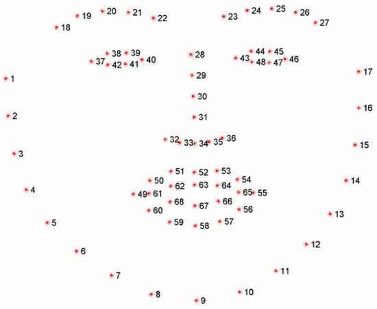
Figure 5.
Illustration of 68 facial keypoints defined in the 300W dataset, covering landmarks on eyebrows, eyes, nose, mouth, and facial contour for precise facial feature localization.
After the initial localization of the pupil center, the next step is to more accurately determine the iris edge. Since the image of the human iris region is often obscured by the upper and lower eyelids, direct edge detection methods may not be sufficient to accurately identify the true edge of the iris. Therefore, this paper employs edge detection technology based on the ray casting method, combined with the direction information of the human eye, to improve the accuracy of iris edge recognition.
The execution of the ray casting method involves determining the eye direction from the eye corner points. First, assume the coordinates of the inner and outer corners of the eye are , respectively. The rotation angle of the eye in the plane is determined based on the eye corner points:
Next, multiple rays are emitted outward from the estimated pupil center, and the rays stop when they encounter a significant gradient change (i.e., the iris edge). This process is completed by analyzing changes in image gray values, effectively distinguishing the true iris edge from the occlusion of the upper and lower eyelids. Assuming the coarse localization coordinates of the pupil center are, the rays are represented by the following Equation (13).
In the equation, represents the step size of the ray, which ranges between the minimum search radius and the maximum search radius , ensuring that the rays cover the entire area from the pupil center to the possible iris edge. The angle of the ray is adjusted based on , allowing the ray to vary within a certain range and cover the entire potential edge area of the iris. As shown in Figure 6, this method can extract more precise key points of the iris edge.
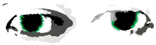
Figure 6.
Results of iris edge point extraction, demonstrating the successful detection of iris boundaries for subsequent pupil center localization.
After ray casting, we obtain a set of iris boundary candidates. We then apply an improved RANSAC circle fitting step to reject outliers caused by eyelid occlusion or specular reflections. In each RANSAC iteration, we randomly sample three boundary points under a side-balanced rule: one point from the left edge set, one from the right edge set, and one from all remaining edge points. This prevents all three points from coming from the same side of the iris, which would generate a degenerate circle.
From the three sampled points we compute a provisional circle (center , radius ). For every detected edge point we then compute its radial residual ; points with residual below a fixed threshold (2 pixels in our setup) are counted as inliers. We repeat this process for a fixed number of iterations (200 in our experiments) and keep the hypothesis with the highest inlier count. Finally, we refit a circle using all inliers of that best hypothesis via least-squares minimization. The center of this final circle is reported as the refined pupil center in pixel coordinates and is later lifted to 3D.
2.2.2. Pupil Center Localization Result Analysis
Through the optimization of the above steps, this study has not only improved the accuracy of pupil localization but also significantly enhanced the processing speed, effectively overcoming the impact of eyelid occlusion. As shown in Figure 7, it can be seen that the algorithm accurately locates the position of the pupil center.
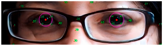
Figure 7.
Pupil center localization results. The result illustrates that the proposed pipeline (landmark-based coarse initialization → ray-casting iris edge extraction → RANSAC + least-squares circle fit) can recover a stable pupil center even with partial eyelid occlusion.
To further verify the accuracy of the pupil center localization algorithm, this paper uses the BioID dataset for experimental analysis. The dataset contains 1521 images from 23 test subjects, with each image having a resolution of 384 × 286 pixels. These images cover a variety of situations, including different facial expressions, diverse lighting conditions, and various head poses.
To quantitatively evaluate the accuracy of pupil center localization, this paper employs a normalized error metric [31], which is based on the maximum distance between the predicted position of the pupil center and the actual position. The calculation formula is (14).
where and represent the Euclidean distances between the predicted and actual positions of the left and right pupil centers, respectively, and is the actual distance between the left and right pupils, used to normalize the error. According to this standard, the smaller the value of , the higher the precision of pupil localization. In the most ideal case, indicates that the predicted pupil center positions almost perfectly coincide with the actual positions.
As shown in Table 3, on the BioID dataset the proposed method achieves 99.3% of test images with normalized error , 97.1% with , and 85.8% with . Here, is the distance between the predicted and ground-truth pupil centers, normalized by the true inter-pupillary distance. These results indicate that the method maintains high localization accuracy even under stricter error thresholds, despite variations in illumination, expression, and partial eyelid occlusion in BioID. Compared with prior eye-center localization methods—Laddi [32], which learns a supervised regression from image-gradient cues; Zhang [33], which targets gaze-gesture pipelines and relies on conventional eye-center heuristics; and Garg [34], which uses Snakuscule active contours and is sensitive to partial eyelid occlusion—our approach differs at three critical stages. First, we seed the coarse pupil center using a two-layer Ensemble of Regression Trees (ERT) for facial landmarks, which reduces drift before fine localization. Second, we extract iris-edge evidence via direction-aware ray casting guided by the inner/outer eye-corner orientation, improving robustness when the upper/lower eyelid occludes the rim. Third, we fit the circle with an edge-side–stratified RANSAC (one point from the left edge, one from the right edge, one random), which suppresses degenerate hypotheses and lowers the iterations needed for consensus, followed by least-squares refinement. Additionally, a PnP-based head-pose gate removes off-frontal frames before measurement, stabilizing errors across poses. Under the same BioID protocol and normalized mean error (NME) metric, these design choices yield higher accuracy than prior work—e ≤ 0.10: 97.1% vs. 92.2–93.6%, and e ≤ 0.05: 85.8% vs. 77.6–85.6% (Table 3)—indicating that the gains arise from the pipeline rather than more training or data.
Table 3.
Pupil center localization accuracy on the BioID dataset. Each column reports the percentage of test images in which the normalized pupil localization error e is below a given threshold. The error e is defined as the Euclidean distance between the predicted and ground-truth pupil centers, normalized by the true inter-pupillary distance. Higher percentages indicate better localization robustness under variations in illumination, expression, and partial eyelid occlusion.
2.3. Lens Segmentation
Pupil and eye-region detection are widely used across domains, including gaze-based human–computer interaction (HCI) and assistive interfaces [35,36], VR/AR eye-tracked foveated rendering [37,38,39,40], driver monitoring and drowsiness detection [41,42], clinical and critical-care quantitative pupillometry, biometric iris recognition, and cognitive workload or affective-state assessment [43,44,45,46]. However, studies that target pupillary height (PH) measurement remain relatively limited. In dispensing practice, PH for each eye is defined as the vertical distance from the pupil center (as seen through the lens) to the lowest point of the corresponding spectacle lens rim. Therefore, to compute PH, it is not sufficient to localize only the pupil center; the system must also accurately segment the spectacle lens and recover the precise coordinates of its lowest rim point. This requirement motivates the dedicated spectacle lens segmentation module described in this section. In 2020, Hao Chen et al. [47] introduced an advanced instance segmentation algorithm named BlendMask, which integrates concepts from Mask R-CNN and YOLACT while incorporating an innovative Blender module. This algorithm delivered cutting-edge results, achieving a peak accuracy of 41.3 AP. Its real-time variant, BlendMask RT, recorded an accuracy of 34.2 mAP with a processing speed of 25 FPS, both outperforming Mask R-CNN. BlendMask has a high processing speed and accuracy, especially performing well under complex backgrounds and diverse eyeglass styles, ensuring the precise localization of the lowest point of the lens, which helps to improve the accuracy of pupillary height measurement. Building upon BlendMask, we propose an RC-BlendMask lens-segmentation module that integrates RCF edge features into the backbone and refines the classification/box/mask losses. The model accurately segments the spectacle lens region and identifies the lowest rim point for PH estimation, whereas PD is computed from the 3D coordinates of the two pupil centers.
2.3.1. BlendMask Network Structure
BlendMask is a cutting-edge, single-stage method for dense instance segmentation that adeptly integrates top-down and bottom-up approaches [47]. Utilizing the innovative anchor-free detection model FCOS [48], the system adeptly extracts intricate low-level features and forecasts instance-level attention with precision by incorporating a novel bottom module. Drawing inspiration from the sophisticated fusion strategies employed in FCIS [49] and YOLACT [50], Hao Chen and other researchers designed the Blender module to more effectively fuse these two types of features.
The architecture of BlendMask consists of two main components: the detector module and the BlendMask module, each playing a critical role in the system’s performance. The BlendMask module is designed with three interconnected sections that work in harmony. The bottom module serves as the foundation, responsible for extracting low-level features and generating a base feature map. Complementing this, the top module is linked to the detector head and focuses on generating the top attention map, which is precisely aligned with the base feature map to ensure accurate feature representation. The blender module acts as the integrative core, seamlessly combining the base feature map with the attention map to maximize functionality and efficiency. This refined structure emphasizes the interconnected roles of the modules, contributing to the enhanced performance and effectiveness of the BlendMask system.
The FCOS detection framework, in conjunction with the multi-scale outputs provided by FPN for object recognition tasks (encompassing bounding box localization and classification scores), employs convolutional tower structures to generate spatial attention. The outputs of FPN are utilized not only for traditional object detection but also for creating spatial attention maps, mathematically represented as , where denotes the batch size, and corresponds to the dimensional embedding of pixel score maps. These maps depict 2D spatial features, typically set at 4 or 8 dimensions, capturing instance-level characteristics such as object shape and orientation. Spatial attention maps are sorted based on classification scores to select the top D proposals, which are subsequently integrated during the fusion process, producing P bounding box predictions and their associated attention metrics A. As shown in Equation (15).
The structure of the bottom module closely resembles that of FCIS and YOLACT, featuring an input dimension of , designed to process low-level feature information.
The extracted characteristics can originate from the backbone network’s low-tier features, the feature pyramid network’s shallow features, or a blend of both. By employing a sequence of decoding processes, which encompass convolution and upsampling operations, a score map, referred to as the base, is constructed. In the provided formula, N designates the batch size, while K signifies the quantity of base maps. H and W represent the input image’s dimensions—height and width, respectively. The output stride of the base map is denoted by s. The core objective of this module is to produce numerous masks for the image, which can then be merged to create an idealized mask. Within this study, the architecture for the bottom branch incorporates the DeepLabV3+ decoder framework, as illustrated in Figure 8. Given that the bottom branch is designed for forecasting global semantic information, alternative dense prediction modules could theoretically fulfill the role of the bottom branch’s structure.
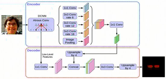
Figure 8.
Architecture of the DeepLabV3+ network used for semantic segmentation, showing the encoder–decoder structure, atrous spatial pyramid pooling (ASPP) module, and feature fusion strategy.
The Blender module serves as a pivotal part of the BlendMask framework, integrating position-sensitive attention to produce the final output. It accepts the base feature map B from the lower layer, the top-level attention A, and bounding box proposals P from the detection tower. Initially, the ROI pooling operator (ROIPooler) from Mask R-CNN extracts the region of interest (ROI) associated with each bounding box from the base feature map. The extracted ROI is then adjusted to a feature map of dimensions R × R. As shown in Equation (16).
Since the attention map has dimensions of M × M, which is smaller compared to R × R, it must be upsampled and interpolated to match the size R × R. Following this, the softmax function is applied to the enlarged attention map for normalization, yielding the attention weight map. The score map sd undergoes an element-wise multiplication with the corresponding feature map rd, followed by summing the resulting values across all channels to derive the final mask map md. As shown in Equation (17).
2.3.2. RC-BlendMask Algorithm
Edge diffusion is a phenomenon that arises during image segmentation with deep learning models such as BlendMask. It primarily occurs as a result of blurred boundaries, making it challenging to differentiate the foreground from the background at object edges. To compute pupil height, precise identification of the lowest points of the eyeglass lenses is essential. However, edge diffusion can introduce errors in determining these points, thereby compromising the precision of the calculated pupil height. To address this issue, this study introduces a novel neural network algorithm named RC-BlendMask, which incorporates the RCF (Richer Convolutional Features) edge detection network into the Backbone segment of the BlendMask framework. This enhancement is designed to improve edge feature representation in images, ensuring that such features receive more emphasis during the subsequent stages of feature extraction. The RC-BlendMask network structure is illustrated in Figure 9.
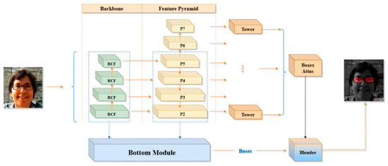
Figure 9.
Structure of the proposed RC-BlendMask network, integrating region-based convolutional features and mask prediction modules for accurate spectacle lens segmentation and pupil localization.
The RCF network (Richer Convolutional Features) is a deep learning model proposed in 2019 for edge detection. It enhances the accuracy of edge prediction by fully utilizing the features from different layers of Convolutional Neural Networks (CNNs). The network structure connects an edge detection sub-network after each convolutional layer, allowing it to capture multi-scale edge information from coarse to fine. By integrating these multi-layer features, RCF is able to output richer and more accurate edge details, improving the performance of edge detection. This method is particularly suitable for high-precision edge detection tasks in the fields of image processing and computer vision. A diagram of its network structure is shown in Figure 10.
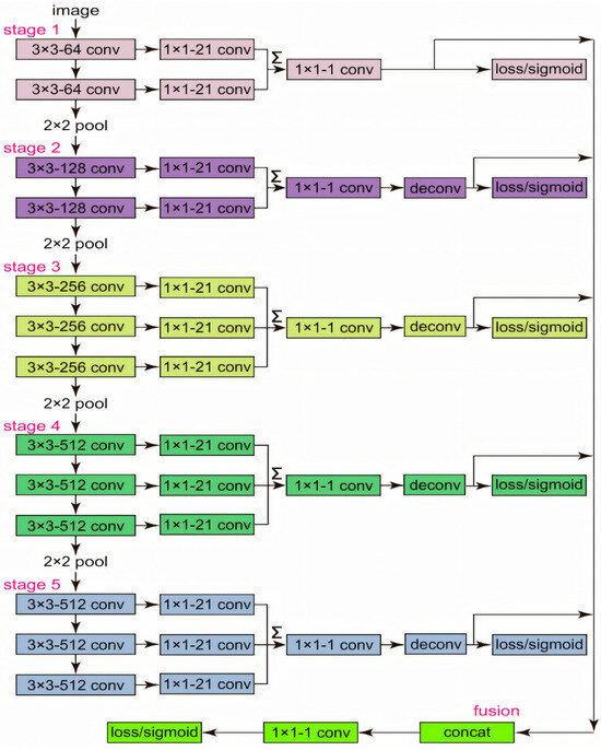
Figure 10.
Diagram of the RCF (Richer Convolutional Features) network, illustrating the multi-scale feature extraction layers and fusion mechanisms for boundary detection tasks.
The original BlendMask uses ResNet101 as its backbone, whereas the RC-BlendMask model incorporates the RCF network into the original BlendMask’s backbone for partial replacement. This integration introduces two possible forward propagation methods: The first method is that the image data passes through the RCF network before being transmitted to ResNet101. The second method is that the image data is processed by RCF and then undergoes a pixel-wise multiplication operation with the original image before continuing to be propagated through the subsequent network. The first method primarily transfers edge information, while the second method essentially enhances the edge information within the image, which is more effective in improving the quality of edge detection. Therefore, this study adopts the second forward propagation method to strengthen the representation of edge information in the image.
We evaluate pixel-level binary lens segmentation (foreground = any lens pixel) with logits thresholded at τ = 0.5 and micro-averaged over all test pixels. From the global confusion matrix (TP, FP, FN, TN), we compute Precision = TP/(TP + FP), Recall = TP/(TP + FN), F1 = 2·TP/(2·TP + FP + FN), IoU = TP/(TP + FP + FN); hence . 95% CIs: Wilson intervals for Precision/Recall/Specificity; bootstrap (image-level, 2000 resamples) for F1/IoU.
Loss Function Design
In this study, the original algorithm’s loss function has been enhanced, resulting in the development of a customized loss function tailored for instance segmentation tasks. This refined loss function is constructed by combining the localization outcomes from object detection with the mask’s segmentation results. As shown in Equation (18).
Among these, represents the classification loss, denotes the localization loss associated with bounding boxes, and corresponds to the segmentation loss for the mask. Parameters θ and α are employed to adjust the relative influence of these losses. In this study, both parameters are assigned a value of 1.
Eyeglass Lens Model Training
We created a manually annotated training set for spectacle lens segmentation. Using the LabelMe tool, annotators drew polygon masks around the left and right spectacle lenses in each image and marked the lens rim, including the lowest point of each lens edge. Each image produced a JSON file containing the pixel coordinates of these polygons.
To ensure consistency, annotators followed written guidelines defining: (i) where the lens boundary ends and the frame begins; (ii) how to handle reflections and glare on the lens surface; and (iii) how to identify the geometric “lowest point” of each lens rim, which is required for pupillary height (PH) computation.
For quality control, 10% of the images were double-labeled independently by a second annotator. We calculated the inter-annotator Intersection over Union (IoU) for the lens masks and reviewed any samples with large discrepancies. A senior annotator then adjudicated and produced the final mask for those cases. Examples of the labeled data and augmented samples are shown in Figure 10, Figure 11 and Figure 12.
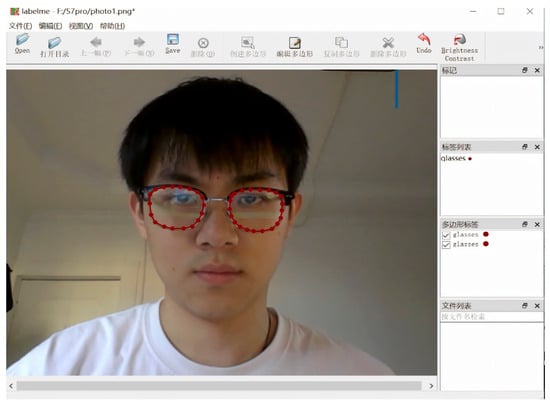
Figure 11.
Interface of the Labelme annotation tool used for manual labeling of spectacle lenses and facial keypoints, including polygonal segmentation and point annotation functions.
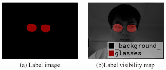
Figure 12.
Example of a visualized annotation image showing labeled spectacle lenses and facial landmarks used for training and evaluation.
This study employs data augmentation techniques to enhance the diversity of image samples, primarily through operations such as flipping and cropping, as illustrated in Figure 13. This approach serves two purposes: it boosts the quantity of experimental samples and mitigates the risk of overfitting.
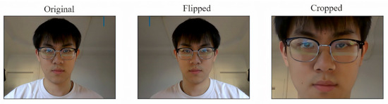
Figure 13.
Samples generated by data augmentation techniques such as rotation, scaling, flipping, and brightness adjustment to enhance the model’s generalization ability.
Figure 14 provides a consolidated view of RC-BlendMask training dynamics over roughly 0–250 k iterations, showing a tight coupling between the learning-rate schedule and the behavior of each loss component. In panel (a), the learning rate exhibits a brief warm-up to its target value, remains flat for the bulk of training, and then undergoes a pronounced step decay around 200 k steps before tapering to a small terminal value; this schedule sets the cadence for convergence observed elsewhere in the figure. The bottom-branch semantic/base loss in panel (b) declines monotonically from the outset—steeply in the early phase, then with diminishing returns around 120–160 k steps—and registers a small but clear additional decrease immediately after the step decay, indicating that global semantic and boundary cues continue to benefit from a lower step size. The classification head in panel (c) converges rapidly: the loss plunges during the first 30–50 k steps and remains near zero thereafter, with only a few narrow transients (e.g., near ~60 k and ~180 k) consistent with hard examples or short-lived batch composition shifts; following the decay, the curve becomes smoother and even closer to its floor. Localization in panel (d) improves more gradually and in a stepwise fashion, which is typical of box regression that refines once classification has stabilized; after the learning-rate drop at ~200 k, there is a noticeable secondary reduction and a lower terminal plateau, reflecting late-stage geometric refinement. The instance mask branch in panel (e) shows a steady, low-variance decline throughout training—from roughly the low-0.03s to well below 0.01—suggesting that segmentation quality tracks the maturing multi-scale features without signs of instability. Aggregating these components, panel (f) shows the total loss decreasing from about 0.64 to ~0.61, with fine-grained improvements through the middle of the run and a synchronized, modest dip at the decay point before flattening; the dark, smoothed trace stays well within the light variability band, and no prolonged oscillations or divergence are observed. Taken together, the figure reflects a well-tuned and stable optimization: the schedule change at ~200 k steps produces the expected coordinated improvements, the classification branch reaches near-floor values early, and the localization and mask branches continue to accrue gains into the late stage, yielding an overall training trajectory that is consistent, efficient, and convergent.
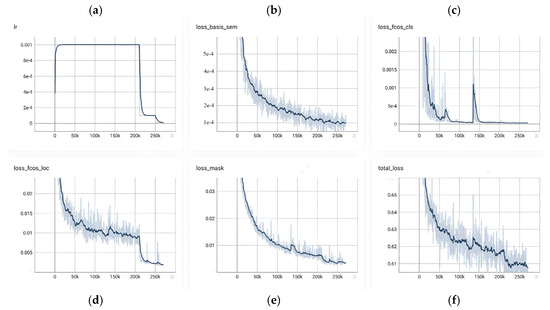
Figure 14.
Relationship between loss value and training epochs, illustrating the model’s convergence behavior and optimization process over time.
Analysis of the Segmentation Results for the Eyeglass Lens Model
The trained lens instance segmentation model effectively predicts the location and dimensions of eyeglass lenses in facial images and determines the coordinates of their lowest point. To visually illustrate the model’s detection outcomes, a selection of images was chosen for presentation. Figure 15 highlights the model’s remarkable ability to segment and identify the region occupied by the glasses accurately, successfully mitigating the negative effects induced by edge diffusion.
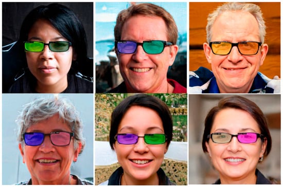
Figure 15.
Lens detection results using the proposed RC-BlendMask model, showing accurate segmentation of spectacle lens regions under various head poses and lighting conditions.
To further assess the algorithm’s capability to segment eyeglass lenses, a series of lens detection experiments were conducted. The segmentation performance of models trained using the original BlendMask and RC-BlendMask networks was evaluated on a custom dataset of over six hundred facial images featuring diverse eyeglasses. Four key evaluation metrics were employed: Precision , Recall , the F1 Score, and Intersection over Union (IOU). Precision P measures the ratio of accurately predicted positive instances to all instances predicted as positive, whereas Recall R quantifies the proportion of correctly identified positive instances relative to all actual positive instances. The definitions of Precision PP and Recall RR are as shown in Equations (19) and (20).
True Positives () and False Positives () represent the number of positive cases that are correctly and incorrectly identified, respectively. False Negatives () represent the number of negative cases that are misidentified as positive. The comprehensive evaluation metric for precision and recall, the F1 Score, is defined as follows (21).
To thoroughly assess the performance of the model algorithm, the Intersection over Union (IOU) metric was employed to evaluate the precision of the detection outcomes. Its definition is as follows (22).
As depicted in Table 4, the experimental outcomes reveal that our model has achieved an exceptionally high standard in precision, recall, and the composite evaluation metric, boasting figures of 97.5%, 93.8%, and 97.65%, respectively. Furthermore, the Intersection over Union (IoU) metric has soared to an impressive 96.56%, underscoring the model’s remarkable accuracy in target localization. This represents a substantial leap in performance over the pre-enhanced Blendmask algorithm, particularly in its capacity to segment eyeglass lenses. What’s more, the model exhibits a consistent level of excellence across a variety of eyeglass types and styles, demonstrating its commendable robustness even in the presence of complex backgrounds.
Table 4.
Comparison of Model Results Before and After Improvement.
To ensure metric consistency, we evaluate lens segmentation under a unified pixel-level protocol. We provide the global confusion matrix and 95% CIs for Precision/Recall/F1/IoU computed on the existing test set in Table 4. The corrected metrics satisfy , ensuring internal consistency; conclusions remain unchanged.
To avoid unfair cross-dataset comparisons, external SOTA results are shown for context only, quoted as reported on their native benchmarks. Our empirical internal baseline is BlendMask (OFF) vs. RC-BlendMask (ON), evaluated on the same held-out test split and thresholds. Additional toggles that would require re-training third-party models are out of scope for this submission.
Because our task (lens-rim segmentation → PH/PD) and acquisition protocol differ from standard benchmarks, re-training external SOTA for a fair comparison would require redistribution of consent-restricted facial data, which is not permitted. We therefore report one in-domain baseline (BlendMask vs. RC-BlendMask), provide training/inference specifics for reproducibility, and include published SOTA numbers strictly as context, not as direct competitors.
2.4. Head Pose Estimation
2.4.1. Head Pose Algorithm Design
Head pose is described by three Euler angles—yaw (left–right rotation), pitch (up–down rotation), and roll (in-plane tilt). We estimate these angles from a single RGB image using a standard Perspective-n-Point (PnP) pipeline:
- (1)
- Facial landmark detection. We first run the trained facial keypoint model (Section 2.1) to obtain 2D image coordinates of anatomically stable points such as eye corners, nose tip, and mouth corners.
- (2)
- 2D–3D correspondence. Each detected 2D keypoint is matched to a predefined 3D face template in canonical head coordinates (e.g., average 3D locations of left eye corner, right eye corner, nose tip, etc.). This gives us pairs {(Xi, Yi, Zi) ↔ (ui, vi)}.
- (3)
- PnP pose solve. Using the camera intrinsics (Section 2.1.5) and these 2D–3D correspondences, we solve the Perspective-n-Point (PnP) problem with OpenCV to estimate the rotation matrix R and translation vector t that align the 3D face model to the observed image.
- (4)
- Euler angle extraction and gating. The rotation matrix R is converted to yaw, pitch, and roll angles. These angles are then compared to predefined thresholds (e.g., |yaw| ≤ 15°, |pitch| ≤ 15°, |roll| ≤ 10°). Frames that exceed the limits are rejected and the subject is prompted to re-center. Only frames within tolerance are used for pupillary distance (PD) and pupillary height (PH) measurement.
This procedure ensures that PH/PD are only computed from near-frontal views, reducing geometric bias due to head tilt.
The orientation of the head in the input image plays a crucial role in determining pupil positioning and locating the lowest point of the eyeglass lenses, which significantly influences the precision of pupillary distance measurements. In the context of computer vision, an object’s pose describes its alignment and spatial positioning relative to the camera. This alignment can change either by adjusting the object’s position or altering the camera’s angle in relation to the object. In three-dimensional geometry, an object’s rotation is typically expressed using three Euler angles: α for the yaw angle, β for the roll angle, and γ for the pitch angle of the head orientation, as illustrated in Figure 16.
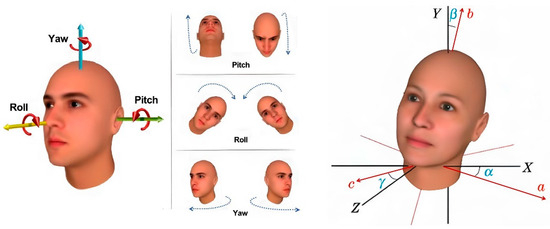
Figure 16.
Definition of head Euler angles (yaw, pitch, and roll) used to describe three-dimensional head orientation in the head pose estimation process.
To precisely determine the head pose in relation to the camera, we have developed an algorithm that adheres to the methodology outlined in Figure 17. This methodology commences with the deployment of a facial keypoint detection model, which has been meticulously trained using the aforementioned ensemble of regression trees. The objective is to pinpoint and extract the precise coordinates of key facial features, including the eyes, nose, mouth, and additional facial landmarks.
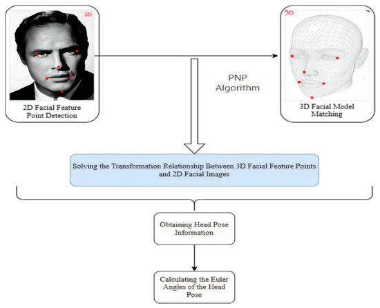
Figure 17.
Flowchart of the head pose estimation algorithm, showing the steps from facial landmark detection to PnP-based 3D head orientation calculation.
Following the extraction of facial features, these landmarks are then correlated with a pre-defined 3D facial model to establish a precise one-to-one correspondence between the 3D facial feature points and the 2D facial image. This critical step is accomplished by addressing the 3D to 2D mapping challenge, specifically leveraging the Perspective-n-Point (PNP) algorithm as implemented in the OpenCV library. The deployment of the PNP algorithm facilitates the reconstruction of the 3D scene’s structural information from a 2D image, thereby furnishing the essential geometric correlations required for accurate head pose estimation [50].
By leveraging this transformational association, critical details about the head orientation can be extracted. Ultimately, through the application of the rotation matrix, the Euler angles defining the head’s spatial alignment are determined. This step signifies the completion of the process for estimating the head pose relative to the camera.
2.4.2. Display of Head Pose Estimation Results
Subsequently, a curated selection of 15 images showcasing various angles was utilized, and the carefully trained head pose estimation model was applied. The algorithm’s predicted head poses were then compared to their true orientations. The results from the experiments demonstrate that, in most cases, the model can accurately identify whether the head is tilted and determine the degree of tilt. A visual illustration of this head pose estimation process is provided in Figure 18.
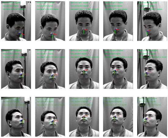
Figure 18.
Head pose estimation results visualized on test images, demonstrating the estimated 3D head orientation vectors overlaid on the detected facial regions.
In order to assess the precision of our head pose estimation algorithm, we conducted rigorous testing on the 300W-LP and AFLW2000 datasets. These datasets are pivotal in the domain of head pose estimation, offering a substantial collection of annotated images that capture a multitude of head poses across a spectrum of angles. They furnish an extensive array of data suitable for both training and evaluation purposes. The datasets are instrumental in gauging the model’s efficacy under a variety of angles and lighting scenarios. By subjecting the model to tests on both datasets, we can effectively ascertain the algorithm’s accuracy and robustness. For each image in these datasets, we compared the predicted yaw, pitch, and roll angles from our PnP-based solver to the annotated ground-truth pose angles provided by the dataset. The mean absolute error (MAE), defined in Equation (23), was computed in degrees for each axis. The values reported in Table 5 are exactly these MAE values (lower is better), which quantify how closely our estimated head pose matches the labeled head pose.
Table 5.
Test Results on Different Datasets.
In this paper, the Mean Absolute Error (MAE) is defined as follows: Given a set of trained facial images A and their corresponding head pose labels B, and the head poses predicted by the algorithm as C, the MAE is defined as (23).
As delineated in Table 5, our head pose estimation algorithm has demonstrated remarkable accuracy, with the Mean Absolute Error (MAE) for the Yaw, Pitch, and Roll axes on both datasets attaining commendably low error rates. The performance on the 300W-LP dataset notably surpassed that of the AFLW2000 dataset. This disparity may stem from the fact that the 300W-LP dataset encompasses a broader range of high-quality annotated images, which facilitates more effective learning and generalization of head pose estimation by the model. In summary, the precision delivered by this head pose estimation algorithm aligns with the stringent accuracy benchmarks of our system.
After acquiring information on the head pose, a series of evaluations were performed to assess how varying head tilt angles affect the precision of pupil distance and height measurements. To guarantee reliable results from these evaluations, specific threshold standards were established. In particular, when the head tilt angle falls within the ranges of −15° ≤ α ≤ 15°, −15° ≤ β ≤ 15°, and −10° ≤ γ ≤ 10°, the measurements are deemed accurate and fall within an acceptable margin of error. If the angles exceed these thresholds, the results are considered unreliable. By applying these criteria, measurements are taken only when the head pose meets the defined standards, thus enhancing the accuracy and dependability of the data while reducing errors caused by head tilt. This approach improves the reliability of the overall measurement outcomes.
2.4.3. Pupil Height and Pupil Distance Measurement Algorithm
After pupil center localization and lens segmentation, we obtain 3D coordinates (in millimeters) for three key points:
- –
- the left pupil center;
- –
- the right pupil center;
- –
- the lowest point on each spectacle lens rim.
These physical coordinates are recovered by (i) fitting the iris boundary with our ray-casting + RANSAC + least-squares circle procedure (Section 2.2) to get each pupil center in pixel space, (ii) segmenting the spectacle lens rim with RC-BlendMask and extracting its lowest point, and (iii) converting pixel coordinates to millimeters on the lens plane using the calibrated camera intrinsics and PnP-based pose (Section 2.1.5).
Pupillary distance (PD) is then defined as the 3D Euclidean distance between the left and right pupil centers. This is given in Equation (24) and is reported in millimeters.
Pupillary height (PH) is defined for each eye as the vertical distance from the pupil center to the lowest point of the corresponding spectacle lens rim. Operationally, PH is computed in the lens plane by measuring the in-plane offset between the pupil center and the lowest rim point on the same side; this is given in Equation (25). PH is also reported in millimeters.
These definitions match dispensing practice, where PD is used to align lens optical centers horizontally, and PH (sometimes called fitting or segment height) is used to position the lens vertically within the frame.
Through the use of facial key points to localize the eye region, an enhanced RANSAC procedure is applied to extract reliable iris edge points. The iris contour is then fitted using a least-squares circle model, and the circle center is taken as the pupil center. This yields the 3D coordinates of the left pupil center and the right pupil center . The interpupillary distance (PD) is computed in 3D as the Euclidean distance between these two centers, as shown in Equation (24).
Using the RC-BlendMask segmentation module, the system also extracts the rim of each spectacle lens and determines the lowest point on each lens edge, with coordinates . In dispensing practice, pupillary height (PH) for each eye is defined as the vertical distance from the pupil center (as seen through the lens) to the lowest point of the corresponding spectacle lens rim. Because PH is measured in the lens plane, only the in-plane offset is required. The resulting PH is obtained using Equation (25).
In summary, the research on this algorithm provides a comprehensive and solid technical foundation for the high-precision measurement of pupillary distance and pupillary height. The proposed algorithms have demonstrated outstanding performance and reliability in practical applications, laying the groundwork for the further development of intelligent measurement systems.
2.4.4. Statistical Analysis
We assessed agreement and reliability for pupillary distance (PD) and pupillary height (PH-L, PH-R) as follows.
Bland–Altman analysis. We computed the mean difference (bias) and 95% limits of agreement (LOA) as
where are paired differences and their SD. We report 95% CIs for the bias and LOA using the Bland–Altman method and inspected proportional bias by regressing on the pairwise mean (lope with 95% CI). In presence of heteroscedasticity, we also examined analyses on the log scale (ratio LOA).
Concordance and intraclass correlation. We report Lin’s CCC with 95% CIs, and ICC with 95% CIs per Shrout & Fleiss/McGraw & Wong conventions. For inter-operator agreement we used ICC(2, 1) (two-way random effects, absolute agreement, single measurement). For test–retest we used ICC(3, 1) (two-way mixed effects, absolute agreement), following reporting guidelines.
Error summaries. We computed mean absolute error (MAE) and root mean squared error (RMSE) relative to the reference device:
Repeatability. For repeated measurements, we estimated the within-subject SD , the repeatability coefficient , and CV% . We report test–retest (same operator, two sessions) and inter-operator (two operators, same session) repeatability separately.
Uncertainty and CIs. Normality was assessed by visual inspection (Q–Q plots) and Shapiro–Wilk tests; when doubtful or sample size was modest, BCa bootstrap (1000 resamples) was used for CIs of CCC/ICC and LOA. All metrics are reported for PD, PH-L, and PH-R.
3. Results
Following the synthesis of the aforementioned research, we conducted a detection and comparative experiment on the intelligent measurement system, which incorporates the algorithm designed for the precise measurement of pupillary height and distance. The i. Terminal2 device (Carl Zeiss AG, Guangzhou, China), recognized for its high-precision measurement capabilities, was employed as a benchmark to assess the performance of our intelligent system. The results of the experiment underscored the system’s superior accuracy and practicality.
To evaluate measurement accuracy, we collected data from 30 adult volunteers. Recruitment was done by convenience sampling at a single site; no pediatric subjects were included. We did not attempt to enforce demographic balance, so this group should not be interpreted as statistically representative of the general population. Each subject was imaged while wearing their own spectacles (with different frame geometries and coatings). Images were acquired with a fixed consumer camera mounted approximately 30 cm from eye level. During acquisition, each subject sat in front of a fixed consumer camera at approximately 30 cm under a consistent indoor lighting setup to reduce glare and strong reflections on the spectacle lenses. No head restraint was used. The system automatically estimated head pose (yaw, pitch, roll) from facial landmarks using a PnP-based solver. Frames in which any Euler angle exceeded predefined thresholds (approximately ±15° yaw/roll and ±10° pitch) were rejected and a new frontal frame was captured. In other words, instead of forcing strict fixation, we allowed natural behavior and simply discarded off-angle frames. This pose-gating procedure is the same mechanism used later in the measurement pipeline.
In addition to utilizing our intelligent measurement system, the Zeiss i.Terminal2, renowned for its precision, was employed to measure pupillary distance and height. The measurements obtained from the i.Terminal2 served as the benchmark for assessing the accuracy of our system. This comparative analysis allowed us to precisely evaluate and analyze the discrepancies between our intelligent measurement system and the industry’s high-precision standards, thereby ensuring the reliability and efficacy of the methods described in this paper for practical use. Such a rigorous comparative analysis is essential for the ongoing refinement and enhancement of the intelligent measurement system. Some measurement data are shown in Table 6.
Table 6.
Pupillary height and pupillary distance measurement results (unit: mm).
To graphically illustrate the discrepancies between the outcomes of the two measurement methodologies, the data are plotted for all subjects as shown in Figure 19. The findings from the proposed intelligent measurement system closely align with those of the i.Terminal2, underscoring the high precision of the system’s measurements. We then performed a quantitative agreement analysis between the two methods. For each metric—interpupillary distance (PD), left pupillary height (PH-L), and right pupillary height (PH-R)—we computed the mean difference between the two systems, the corresponding standard deviation, the 95% Bland–Altman limits of agreement, and the maximum absolute difference across the 30 participants. These results are summarized in Table 7. Overall, the average measurements from both systems are largely congruent, with the proposed system giving slightly higher values on average, and the observed dispersion (standard deviation) and 95% limits of agreement remaining within clinically acceptable tolerances.
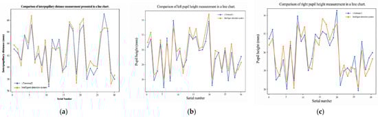
Figure 19.
Comparison between the proposed method and a commercial i.Terminal2 device in measuring pupillary distance (PD) and pupil height (PH), highlighting measurement accuracy and consistency: (a) Interpupillary distance (IPD) measurement comparison for 30 subjects. (b) Left pupil height measurement comparison. (c) Right pupil height measurement comparison.
Table 7.
Summary of agreement between the proposed system and the commercial reference device (Zeiss i.Terminal2) for interpupillary distance (PD) and pupillary height (PH-L, PH-R). For each metric we report: the mean value measured by each method (in mm), the mean difference between methods, the standard deviation (SD) of that difference, and the maximum absolute difference observed across 30 participants. Lower mean difference and SD indicate closer agreement.
The mean difference and standard deviation between the two methods are both less than 1.5 mm, which is considered an acceptable margin of error. The highest deviation in pupillary distance measurement was observed in the 16th experimental group, potentially due to anomalies during the image capture process. Nevertheless, this error remains within an acceptable range. This finding reaffirms the proximity of the results between the two measurement methods.
Employing the measurement data from the i.Terminal2 as the benchmark, we conducted a consistency analysis experiment on our visual intelligent measurement system. The experiment commenced with a correlation assessment to determine the linear relationship between the results derived from both measurement methods. The calculated data revealed a Pearson correlation coefficient of 0.944 for pupillary distance, 0.964 for the left pupillary height, and 0.916 for the right pupillary height. These figures all indicate a robust positive correlation. This finding suggests a highly linear relationship between the measurement outcomes of the visual intelligent measurement system and the i.Terminal2, thereby offering substantial statistical validation for the reliability of its measurement results.
A Bland–Altman analysis was performed to evaluate the concordance between the two measurement techniques. This approach adeptly exposes the extent of measurement discrepancies and any systematic bias by graphing the disparity between the two methods’ results against their mean values. The data presented in Figure 19a discloses that the 95% confidence interval for pupillary distance extends from −2.00 mm to 2.70 mm. This indicates that 95% of the measurement discrepancies fall within this range, suggesting a high degree of concordance between the two measurement techniques. Furthermore, as illustrated in Figure 19b,c, the 95% confidence interval for the left pupillary height is between −0.84 mm and 1.76 mm, while for the right pupillary height, it spans from −1.85 mm to 1.79 mm. These findings underscore the significant consistency in pupillary height measurements between our visual intelligent measurement system and the i.Terminal2.
Visual inspection of the graph indicates that the majority of measurement differences are tightly clustered around the mean difference line, with no discernible systematic bias or trend variation associated with the magnitude of the measurement values. This observation further substantiates the visual intelligent measurement system’s strengths in terms of consistency and reliability.
Determining the relative error is a pivotal analytical technique for assessing the precision of measurement data, as it quantifies the proportion of each measurement deviation in relation to a reference value—the i.Terminal2 measurement outcomes, in this case. In our experiment, we computed the relative errors for both the pupillary distance and height measurements. Figure 20a demonstrates that the intelligent measurement system attained an average relative error of 1.81% in pupillary distance measurements. Regarding pupillary height, as depicted in Figure 20b,c, the average relative error was 2.51% for the left eye and 2.96% for the right eye. In absolute terms, our mean absolute differences versus i.Terminal2 were 0.73 mm (PH-L), 0.89 mm (PH-R), and 1.13 mm (PD) (Table 7). Standards for mounted lenses indicate ±1.0 mm tolerance for segment/fitting-cross vertical location (per lens) and limits on unwanted prism of ≤0.67Δ horizontal and ≤0.33Δ vertical, with an additional requirement that the prism reference point (PRP) not deviate by more than 1.0 mm from its specified position (ANSI Z80.1; see also ISO 21987) [51,52]. By Prentice’s rule (Δ = F·c, with c in cm), a 0.5 mm monocular centration error (0.05 cm) in a ±3.00 D lens induces ~0.15Δ, and ~0.30Δ at ±6.00 D, both within the above tolerances [53]. Interpreting our PD difference (1.13 mm) as ~0.56 mm per eye when symmetrically distributed, the implied unwanted prism at typical powers remains within tolerance. Therefore, the observed PH and PD discrepancies are clinically acceptable under standard centration and prism criteria, while we note that higher-powered prescriptions reduce the decentration margin (per Prentice’s rule). Outliers (PD in groups 16 and 29; PH-L in groups 12 and 22) were analyzed for capture artifacts (lighting/gaze/pose) and remain within the 95% Bland–Altman limits (Figure 20), At the same time, the relative error of this method is controlled between 3% and 4% (Figure 21).
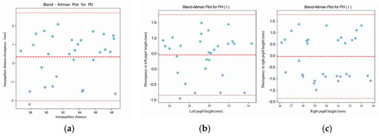
Figure 20.
Bland–Altman analysis results evaluating the agreement between the proposed method and the reference device for PD and PH measurements: (a) Interpupillary distance (IPD) analysis. (b) Left pupil height (PH-L) analysis. (c) Right pupil height (PH-R) analysis.
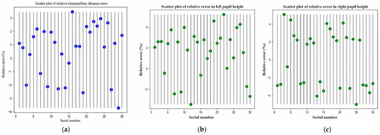
Figure 21.
Relative error analysis of the proposed method compared to the reference de-vice, showing error distribution and statistical indicators: (a) Interpupillary distance (IPD) relative error for 30 subjects. (b) Left pupil height (PH-L) relative error. (c) Right pupil height (PH-R) relative error.
Upon conducting an exhaustive analysis of the experimental data, our visual intelligent measurement system has exhibited commendable precision, underscoring its substantial practical utility in the realm of pupillary height and distance measurement. Future research endeavors should concentrate on refining the algorithms and measurement protocols of the intelligent system. This optimization aims to curtail measurement errors and bolster its precision and dependability across diverse scenarios. The experimental outcomes affirm that this intelligent detection system has attained a high caliber of precision and practicality.
4. Discussion
This work presents a vision-based system for the automatic measurement of pupillary height (PH) and pupillary distance (PD) that integrates a two-layer Ensemble of Regression Tree (ERT) for robust landmarking, direction-aware ray casting guided by eye-corner orientation to recover informative iris edges under eyelid occlusion, an edge-side-stratified RANSAC followed by least-squares circle fitting for sub-pixel pupil-center refinement, and a PnP-based head-pose gate to exclude off-frontal frames prior to measurement. Relative to representative eye-center localization baselines (gradient-driven supervised regression, gaze-pipeline heuristics, and Snakuscule active contours), the proposed pipeline differs at three critical stages—coarse seeding, edge evidence gathering, and hypothesis sampling—and produces higher accuracy on BioID under the same NME protocol (e ≤ 0.10: 97.1% vs. 92.2–93.6%; e ≤ 0.05: 85.8% vs. 77.6–85.6%; Table 3), indicating that the gains arise from algorithmic design rather than additional training alone.
In this study, robustness refers to (i) stability of the automatic measurements across subjects and repeated captures, (ii) tolerance to moderate variation in head pose and illumination, and (iii) agreement with an external clinical reference. We quantify robustness using Bland–Altman bias and 95% limits of agreement, Pearson correlation, mean absolute error and RMSE against i.Terminal2, as well as cross-dataset landmark accuracy on 300W and WFLW, which include challenging pose, blur, occlusion, and lighting conditions. Importantly, the observed errors are clinically contextualized. The average relative error was 2.51% for the left eye and 2.96% for the right eye. In absolute terms, mean absolute differences versus i.Terminal2 were 0.73 mm (PH-L), 0.89 mm (PH-R), and 1.13 mm (PD) (Table 7). Tolerances commonly applied to mounted lenses specify ±1.0 mm for segment/fitting—cross vertical location per lens and limits on unwanted prism of approximately were ≤0.67Δ (horizontal) and ≤0.33Δ (vertical) at the prism reference point (ANSI Z80.1; ISO 21987). By Prentice’s rule (Δ = F·c, c in cm), a 0.5 mm monocular centration error (0.05 cm) in a ±3.00 D lens induces ~0.15Δ and ~0.30Δ at ±6.00 D—within those limits. Interpreting our PD difference (1.13 mm) as ~0.56 mm per eye when symmetrically distributed, the implied unwanted prism at typical powers remains within tolerance. Therefore, the PH and PD discrepancies observed here are consistent with clinical acceptability under standard centration and prism criteria, although higher-powered prescriptions naturally reduce the decentration margin. Outliers (PD in groups 16 and 29; PH-L in groups 12 and 22) remained within the 95% Bland–Altman limits (Figure 19) and were traceable to capture artifacts.
The dominant sources of error were (i) suboptimal illumination (noise, overexposure, or flare) that degrades iris–sclera and rim contrast and weakens edge evidence for the ray-casting stage and (ii) residual pose or fixation deviations (slight head tilt or gaze offset) that can bias monocular centration despite pose gating. Retakes with improved lighting and explicit fixation cues reduced the tails of the error distribution without materially changing the mean.
We also recognize potential bias and generalizability limitations. Public landmark datasets used (e.g., 300W, WFLW, BioID) offer pose/expression diversity but lack explicit skin-tone labels and likely under-represent darker skin tones and low-contrast irides, which may affect pupil/iris edge detection and lens-rim segmentation in low-luminance conditions. To mitigate this, future work will expand data collection across Fitzpatrick skin-tone groups and eyewear styles, apply targeted photometric augmentation (luminance/contrast/color jitter) tailored to low-contrast irides, and include external validation on demographically diverse cohorts. Regarding age, the system was not validated in children and is not claimed for pediatric fitting. Pediatric PD varies with age, and cooperation is challenging; planned adaptations include animated fixation targets, short-burst multi-frame capture with temporal stabilization, higher-resolution eye crops for small faces, and pose-gated retakes, with performance reported and stratified by age. Although the pipeline was designed to mitigate glare and contrast loss (via photometric augmentation, edge-aware rim extraction, and pose gating), all quantitative comparisons with the i.Terminal2 were performed under controlled indoor lighting. Therefore, robustness to challenging real-world illumination (e.g., strong reflections, backlighting, outdoor lighting) has not yet been fully validated and remains part of future work.
Practically, the proposed pipeline achieves accuracy comparable to a high-end commercial device while operating with a single camera and commodity compute, enabling a camera-only workflow on commodity hardware that may reduce equipment cost and streamline in-store or tele-optometry capture. Pose gating offers an operational safeguard by prompting retakes when Euler angles exceed thresholds. Remaining limitations include dataset demography and pediatric validation, residual sensitivity to lighting and partial occlusion, and the need for stronger shape/edge priors at the rim–skin interface. Future work will explore transformer/self-attention backbones and graph-enhanced shape priors to further suppress edge diffusion, super-resolution and uncertainty-aware circle fitting to stabilize the pupil center under occlusion, and binocular/multi-camera capture with automated, periodic calibration and on-line illumination normalization to improve robustness across environments. Finally, we plan to release a demographically annotated validation set and report stratified metrics (skin tone, age band, eyewear type) to enable transparent assessment of fairness and generalizability.
While the proposed system achieves clinically acceptable agreement with a high-end commercial device using only a single off-the-shelf camera, several limitations remain. First, performance still depends on illumination quality: glare on the spectacle lens, strong reflections, or underexposure can weaken iris–sclera contrast and degrade RC-BlendMask rim extraction, increasing PH/PD variability. Second, although we apply pose gating via PnP and Euler-angle thresholds, residual head tilt or off-axis gaze can bias monocular centration, and the need to discard off-frontal frames may reduce first-pass capture efficiency in realistic retail environments. Third, our validation cohort (30 participants) did not explicitly stratify for skin tone, iris pigmentation, eyewear style, or pediatric patients; as a result, generalizability to darker irides, highly reflective coatings, or uncooperative children has not yet been established. Finally, we have not exhaustively characterized extreme prescriptions (very high diopters or strong wraparound frames), where decentration tolerances tighten.
Future work will expand the demographic and optical diversity of the dataset, incorporate illumination normalization and glare suppression into the capture pipeline, and explore lightweight multi-view or binocular capture to further stabilize depth and rim geometry without significantly increasing system cost. We will also investigate pediatric-specific protocols (shorter capture windows, animated fixation targets) and report stratified performance metrics for fairness and clinical applicability.
Author Contributions
Conceptualization, S.H. and Z.Y.; methodology, S.H.; software, S.H.; validation, S.H.; formal analysis, S.H.; investigation, S.H. and Z.Y.; resources, H.X.; data curation, S.H.; writing—original draft preparation, S.H.; writing—review and editing, H.X.; visualization, S.H.; supervision, H.X.; project administration, H.X.; funding acquisition, H.X. All authors have read and agreed to the published version of the manuscript.
Funding
This research received no external funding.
Data Availability Statement
All data can be supplied by contract correspondent author, e-mail: parallelunivers@163.com.
Conflicts of Interest
The authors declare no conflicts of interest.
Abbreviations
The following abbreviations are used in this manuscript.
| Abbrev. | Definition |
| 2D | Two-Dimensional |
| 3D | Three-Dimensional |
| 300W | 300 Faces in-the-Wild (dataset) |
| 300W-LP | 300W Large-Pose (dataset extension) |
| AABB | Axis-Aligned Bounding Box |
| AFLW2000 | Annotated Facial Landmarks in the Wild (2000 images) |
| AP | Average Precision |
| AUC | Area Under the Curve |
| ASPP | Atrous Spatial Pyramid Pooling |
| BioID | BioID Face Database |
| CNN | Convolutional Neural Network |
| CPU | Central Processing Unit |
| DeepLabV3+ | DeepLab Version 3 Plus |
| DL | Deep Learning |
| ERT | Ensemble of Regression Trees |
| FCIS | Fully Convolutional Instance-aware Semantic Segmentation |
| FCOS | Fully Convolutional One-Stage (object detector) |
| FPN | Feature Pyramid Network |
| FPS | Frames Per Second |
| FR | Failure Rate (samples exceeding the NME threshold) |
| GPU | Graphics Processing Unit |
| IoU | Intersection over Union |
| IPD | Interpupillary Distance (synonym of PD) |
| MAE | Mean Absolute Error |
| mAP | mean Average Precision |
| NME | Normalized Mean Error |
| OBB | Oriented Bounding Box |
| OpenCV | Open Source Computer Vision Library |
| PD | Pupillary Distance |
| PH | Pupillary Height |
| PnP | Perspective-n-Point (also written PNP) |
| RANSAC | Random Sample Consensus |
| RC-BlendMask | BlendMask enhanced with RCF edge features |
| RCF | Richer Convolutional Features |
| ROI | Region of Interest |
| ROIPooler | Region of Interest Pooling operator |
| RT | Real-Time (suffix used in model names) |
| WFLW | Wider Facial Landmarks in the Wild (dataset) |
References
- Tian, H.; Guan, T.; Cai, M.; Yang, H. Evaluation Model of VDT Visual Comfort Based on Pupil Diameter. Laser Optoelectron. Prog. 2020, 57, 300–306. [Google Scholar] [CrossRef]
- Murray, N.P.; Hunfalvay, M.; Bolte, T. The reliability, validity, and normative data of interpupillary distance and pupil diameter using eye-tracking technology. Transl. Vis. Sci. Technol. 2017, 6, 2. [Google Scholar] [CrossRef]
- Du, Y.; Liu, K.; Ju, Y.; Wang, H. A Comfort Analysis of AR Glasses on Physical Load During Long-Term Wearing. Ergonomics 2022, 66, 21–23. [Google Scholar] [CrossRef]
- Benhaim-Sitbon, L.; Lev, M.; Polat, U. Binocular fusion disorders impair basic visual processing. Sci. Rep. 2022, 12, 12564. [Google Scholar] [CrossRef]
- Schmitz, S.; Krummenauer, F.; Henn, S.; Dick, H.B. Comparison of three different technologies for pupil diameter measurement. Graefe’s Arch. Clin. Exp. Ophthalmol. 2003, 241, 472–477. [Google Scholar] [CrossRef] [PubMed]
- Henley, K.; Kier, P.; McKee, A. Accuracy and Precision of Fitting Measurements with the Zeiss I. Terminal 2. Master’s Thesis, Northeastern State University, Tahlequah, OK, USA, 2016. [Google Scholar]
- Jung, Y.R.; Byoung, S.C. A Comparative Analysis of Interpupillary Distance Measurement Techniques Evaluation in Modern Times: From Rulers to Apps. Clin. Optom. 2024, 16, 309–316. [Google Scholar] [CrossRef] [PubMed]
- Zheng, R.; Xu, G.; Tang, X.; Zhai, L.; Tan, D. Analysis and Comparison of Line of Sight Distance Measurement with Pupillary Distance. Chin. J. Sch. Health 2007, 1, 79. (In Chinese) [Google Scholar]
- Wang, Y. The Positive Significance of Replacing the Pupillary Distance Ruler with a Pupillometer. China Metrol. 2004, 10, 58. (In Chinese) [Google Scholar] [CrossRef]
- Zheng, Y.; Wu, Z.; Zheng, F.; Huang, Z. Design and Implementation of a Pupillary Distance Measurement APP. Comput. Era 2020, 11, 70–74. (In Chinese) [Google Scholar] [CrossRef]
- Vera-Olmos, F.J.; Pardo, E.; Melero, H.; Malpica, N. DeepEye: Deep convolutional network for pupil detection in real environments. Integr. Comput.-Aided Eng. 2019, 26, 85–95. [Google Scholar] [CrossRef]
- Kumar, R.T.; Raja, S.K.; Ramakrishnan, A.G. Eye Detection Using Color Cues and Projection Functions. In Proceedings of the 2002 International Conference on Image Processing, Rochester, NY, USA, 22–25 September 2002; Volume 3, pp. 337–340. [Google Scholar]
- Gu, K.K.; Dong, Y.F.; Zhou, Z.; Liu, M.; Chen, S.; Fu, W.W. Real-time pupil detection based on contour tracking. Curr. Trends Comput. Sci. Mech. Autom. 2017, 2, 31–40. [Google Scholar]
- Lin, S.; Lu, Q.; Wang, S.; Han, P.; Li, J.; Xu, K. Pupil Localization in Non-Ideal Conditions Based on Dilated Full Convolutional Network. Laser J. 2021, 42, 33–38. (In Chinese) [Google Scholar] [CrossRef]
- Li, Y.; Ding, H.; Zhang, L.; Zhao, C.; Zhang, S.; Wang, A. Pupil Diopter Detection Approach Based on Improved YOLOv3. Infrared Technol. 2022, 44, 702–708. (In Chinese) [Google Scholar]
- Sun, Y.; Liu, W.; Jiang, M. Pupil Localization Algorithm Based on Attention Mechanism and Dilated Convolution. Electron. Meas. Technol. 2023, 46, 126–132. (In Chinese) [Google Scholar] [CrossRef]
- Barry, C.; Wang, E. Racially Fair Pupillometry Measurements for RGB Smartphone Cameras Using the Far Red Spectrum. Sci. Rep. 2023, 13, 13841. [Google Scholar] [CrossRef]
- Shen, K.; Li, Y.; Guo, Z.; Gao, J.; Wu, Y. Model-Based 3D Gaze Estimation Using a TOF Camera. Sensors 2024, 24, 1070. [Google Scholar] [CrossRef]
- Ben Barak-Dror, O.; Hadad, B.; Barhum, H.; Haggiag, D.; Tepper, M.; Gannot, I.; Nir, Y. Touchless Short-Wave Infrared Imaging for Dynamic Rapid Pupillometry and Gaze Estimation in Closed Eyes. Commun. Med. 2024, 4, 157. [Google Scholar] [CrossRef]
- Qammaz, A.; Argyros, A.A. A Unified Approach for Occlusion Tolerant 3D Facial Pose Capture and Gaze Estimation Using MocapNETs. In Proceedings of the IEEE/CVF International Conference on Computer Vision Workshops (ICCVW 2023), Paris, France, 2–6 October 2023; IEEE: Piscataway, NJ, USA; pp. 3178–3187. [Google Scholar]
- Chen, M.; Zhao, Y.; Yang, W.; Qian, J.; Li, S.; Zheng, Y.; Ma, J.; Wang, S.; Chen, J.; Wei, J. A Model for Suppressing Stray Light in Astronomical Images Based on Deep Learning. Sci. Rep. 2024, 14, 27521. [Google Scholar] [CrossRef]
- Clermont, L.; Adam, G. Using Deep Learning for Effective Simulation of Ghost Reflections. Results Opt. 2024, 15, 100643. [Google Scholar] [CrossRef]
- Zhu, X.; Lei, Z.; Liu, X.; Shi, H.; Li, S.Z. Face Alignment Across Large Poses: A 3D Solution. In Proceedings of the IEEE Conference on Computer Vision and Pattern Recognition (CVPR), Las Vegas, NV, USA, 27–30 June 2016; pp. 146–155. [Google Scholar]
- Kowalski, M.; Naruniec, J.; Trzcinski, T. Deep Alignment Network: A Convolutional Neural Network for Robust Face Alignment. In Proceedings of the IEEE Conference on Computer Vision and Pattern Recognition Workshops (CVPRW), Honolulu, HI, USA, 21–26 July 2017; pp. 2034–2043. [Google Scholar]
- Feng, Z.-H.; Kittler, J.; Christmas, W.; Handa, A.; Jourabloo, A. Wing Loss for Robust Facial Landmark Localisation with Convolutional Neural Networks. In Proceedings of the IEEE Conference on Computer Vision and Pattern Recognition (CVPR), Salt Lake City, UT, USA, 18–23 June 2018; pp. 2235–2245. [Google Scholar]
- Wang, X.; Bo, L.; Li, F. Adaptive Wing Loss for Robust Face Alignment via Heatmap Regression. In Proceedings of the IEEE/CVF International Conference on Computer Vision (ICCV), Seoul, Republic of Korea, 27 October–2 November 2019; pp. 6971–6981. [Google Scholar]
- Bulat, A.; Tzimiropoulos, G. How Far Are We from Solving the 2D & 3D Face Alignment Problem? (and a Dataset of 230,000 3D Facial Landmarks). In Proceedings of the IEEE International Conference on Computer Vision (ICCV), Venice, Italy, 22–29 October 2017; pp. 1021–1030. [Google Scholar]
- Kazemi, V.; Sullivan, J. One Millisecond Face Alignment with an Ensemble of Regression Trees. In Proceedings of the IEEE Conference on Computer Vision and Pattern Recognition (CVPR), Columbus, OH, USA, 23–28 June 2014; pp. 1867–1874. [Google Scholar]
- Sagonas, C.; Antonakos, E.; Tzimiropoulos, G.; Zafeiriou, S.; Pantic, M. 300 Faces in-the-Wild Challenge: Database and Results. Image Vis. Comput. 2016, 47, 3–18. [Google Scholar] [CrossRef]
- Wu, W.; Qian, C.; Yang, S.; Wang, Q.; Cai, Y.; Zhou, Q. Look at Boundary: A Boundary-Aware Face Alignment Algorithm. In Proceedings of the IEEE Conference on Computer Vision and Pattern Recognition (CVPR), Salt Lake City, UT, USA, 18–23 June 2018; pp. 2129–2138. [Google Scholar]
- Cai, H.; Liu, B.; Zhang, J.; Chen, S.; Liu, H. Visual Focus of Attention Estimation Using Eye Center Localization. IEEE Syst. J. 2017, 11, 1320–1325. [Google Scholar] [CrossRef]
- Laddi, A.; Prakash, N.R. An Augmented Image Gradients Based Supervised Regression Technique for Iris Center Localization. Multimed. Tools Appl. 2016, 76, 7129–7139. [Google Scholar] [CrossRef]
- Zhang, Z.; Smith, M.L.; Smith, L.N.; Farooq, A. Eye Center Localization and Gaze Gesture Recognition for Human–Computer Interaction. J. Opt. Soc. Am. A 2016, 33, 314–325. [Google Scholar] [CrossRef]
- Garg, S.; Tripathi, A.; Cutrell, E. Accurate Eye Center Localization Using Snakuscule. In Proceedings of the IEEE Winter Conference on Applications of Computer Vision, Lake Placid, NY, USA, 7–9 March 2016; IEEE: Piscataway, NJ, USA; pp. 1–8. [Google Scholar]
- Chen, A.; Liu, W.; Zhang, R.; Lei, J.; Li, L.; Fang, Y. Real-Time Human–Computer Interaction Using Eye Gazes. Manuf. Lett. 2023, 37, 74–77. [Google Scholar] [CrossRef]
- Dondi, P.; Porta, M. Gaze-Based Human–Computer Interaction for Museums and Exhibitions: Technologies, Applications and Future Perspectives. Electronics 2023, 12, 3064. [Google Scholar] [CrossRef]
- Adhanom, I.B.; MacNeilage, P.; Folmer, E. Eye Tracking in Virtual Reality: A Broad Review of Applications and Challenges. Virtual Real. 2023, 27, 1481–1505. [Google Scholar] [CrossRef] [PubMed]
- Kim, J.; Kim, J.; Jung, M.; Kwon, T.; Kim, K.K. Individualized Foveated Rendering with Eye-Tracking Head-Mounted Display. Virtual Real. 2024, 28, 25. [Google Scholar] [CrossRef]
- Al-Quraishi, M.S.; Ali, S.S.A.; Al-Qurishi, M.; Tang, T.B.; Elferik, S. Technologies for Detecting and Monitoring Drivers’ States: A Systematic Review. Heliyon 2024, 10, e39592. [Google Scholar] [CrossRef]
- Florez, R.; Palomino-Quispe, F.; Alvarez, A.B.; Coaquira-Castillo, R.J.; Herrera-Levano, J.C. A Real-Time Embedded System for Driver Drowsiness Detection Based on Visual Analysis of the Eyes and Mouth Using Convolutional Neural Network and Mouth Aspect Ratio. Sensors 2024, 24, 6261. [Google Scholar] [CrossRef]
- Ali, A.M.S.; Gul, W.; Sen, J.; Hewitt, S.-J.; Olubajo, F.; McMahon, C. Evaluating the Utility of Quantitative Pupillometry in a Neuro-Critical Care Setting for Monitoring Intracranial Pressure: A Prospective Cohort Study. Clin. Neurol. Neurosurg. 2024, 239, 108215. [Google Scholar] [CrossRef]
- Vrettou, C.S.; Tzerefos, C.; Tzoufi, M.; Lappa, E.; Giannopoulos, C.; Gavrielatou, E. The Role of Automated Infrared Pupillometry in Traumatic Brain Injury. J. Clin. Med. 2024, 13, 614. [Google Scholar] [CrossRef]
- Chen, W.; Tang, M.; Jin, Y.; Chen, L.; Lin, J.; Yang, X. Automated ultrasonographic pupillary assessment: A New Neuro-Ophthalmological Assessment Tool. J. Int. Med. Res. 2024, 52, 3000605241299927. [Google Scholar] [CrossRef]
- Nguyen, K.; Proença, H.; Alonso-Fernandez, F. Deep Learning for Iris Recognition: A Survey. ACM Comput. Surv. 2024, 56, 1–35. [Google Scholar] [CrossRef]
- Ma, X.; Monfared, R.; Grant, R.; Goh, Y.M. Determining Cognitive Workload Using Physiological Measurements: Pupillometry and Heart-Rate Variability. Sensors 2024, 24, 2010. [Google Scholar] [CrossRef] [PubMed]
- Alshanskaia, E.I.; Portnova, G.V.; Liaukovich, K.; Martynova, O.V. Pupillometry and Autonomic Nervous System Responses to Cognitive Load and False Feedback: An Unsupervised Machine Learning Approach. Front. Neurosci. 2024, 18, 1445697. [Google Scholar] [CrossRef] [PubMed]
- Chen, H.; Sun, K.; Tian, Z.; Shen, C.; Huang, Y.; Yan, Y. BlendMask: Top-Down Meets Bottom-Up for Instance Segmentation. In Proceedings of the IEEE/CVF Conference on Computer Vision and Pattern Recognition (CVPR), Seattle, WA, USA, 13–19 June 2020; pp. 8573–8581. [Google Scholar]
- Truong, L.N.H.; Clay, E.; Mora, O.E.; Cheng, W.; Singh, M.; Jia, X. Rotated mask region-based convolutional neural network detection for parking space management system. Transp. Res. Rec. 2023, 2677, 1564–1581. [Google Scholar] [CrossRef]
- Tian, Z.; Shen, C.; Chen, H.; He, T. FCOS: Fully Convolutional One-Stage Object Detection. In Proceedings of the IEEE/CVF International Conference on Computer Vision (ICCV), Seoul, Republic of Korea, 27 October–2 November 2019; pp. 9627–9636. [Google Scholar]
- Li, Y.; Qi, H.; Dai, J.; Ji, X.; Wei, Y. Fully Convolutional Instance-Aware Semantic Segmentation. In Proceedings of the IEEE Conference on Computer Vision and Pattern Recognition (CVPR), Honolulu, HI, USA, 21–26 July 2017; pp. 2359–2367. [Google Scholar]
- ANSI Z80.1-2020; Quick Reference Guide—Prescription Ophthalmic Lenses. The Vision Council: Alexandria, VA, USA, 2020.
- ISO 21987:2017; Ophthalmic Optics—Mounted Spectacle Lenses. 2nd ed. ISO: Geneva, Switzerland, 2017.
- Kaur, K.; Gurnani, B. Prisms. In StatPearls; StatPearls Publishing: Treasure Island, FL, USA, 2023. [Google Scholar]


Disclaimer/Publisher’s Note: The statements, opinions and data contained in all publications are solely those of the individual author(s) and contributor(s) and not of MDPI and/or the editor(s). MDPI and/or the editor(s) disclaim responsibility for any injury to people or property resulting from any ideas, methods, instructions or products referred to in the content. |
© 2025 by the authors. Published by MDPI on behalf of the International Institute of Knowledge Innovation and Invention. Licensee MDPI, Basel, Switzerland. This article is an open access article distributed under the terms and conditions of the Creative Commons Attribution (CC BY) license (https://creativecommons.org/licenses/by/4.0/).