A Tri-Level Distributionally Robust Defender–Attacker–Defender Model for Grid Resilience Enhancement Under Repair Time Uncertainty

Abstract

Extreme damage poses a serious challenge to the safe operation of power grids. Optimizing the allocation of defense resources to improve the grid’s disaster resistance capabilities is the main concern of the power system. In this paper, a distributed robust optimal defense resource allocation method based on the defender–attacker–defender model is proposed to improve the disaster resilience of power grids. This method takes into account the uncertainty of restoration time due to different damage intensities and improves the efficiency of restoration resource scheduling in the restoration process. Meanwhile, a set covering-column and constraint generation (SC-C&CG) algorithm is proposed for the case that the mixed integer model does not satisfy the Karush–Kuhn–Tucker (KKT) condition. A case study based on the IEEE 24-bus system is conducted, and the results verify that the proposed method can minimize the system dumping load under the uncertainty of the maintenance time involved.

1. Introduction

A number of low-probability, high-impact events, such as extreme disasters, episodic failures, and deliberate attacks, are threatening the stable operation of power systems. In 2012, Hurricane Sandy damaged the distribution system in New York State, USA, and more than eight million customers suffered power outages [1]. The Ukrainian power grid was deliberately attacked in 2015, leaving a large number of residents without power for several hours [2]. Heavy rains in Zhengzhou, China, in 2021 disrupted more than 500 power lines and knocked out power to more than 400 neighborhoods [3]. Enhancing the resilience of distribution systems to extreme events has received widespread attention.

The ability of the power system to withstand extreme events and quickly restore power is referred to as resilience [4]. Resilience is defined primarily through vulnerability and recoverability. Vulnerability refers to the loss of power system load shedding suffering disruptive events, while recoverability refers to the repair speed at which the power system returns to normal operation after disruption [5]. These involve two periods: pre-disaster protection and post-disaster restoration. In general, measures for pre-disaster protection include reinforcing transmission lines [6], reinforcing nodes [7], deploying distributed generators [8], etc. Post-disaster restoration measures include repairing lines and nodes [9], reconfiguring topology [10], dispatching mobile emergency generators (MEG) [11], and more.

For confined power networks like ships, a centralized emergency control strategy is proposed to manage disturbances in multi-terminal Voltage–Source–Converter (VSC)-based power systems [12]. In [13], strategies to enhance power system resilience against high-impact low-probability (HILP) events are reviewed, focusing on safeguarding systems with high renewable penetration.

Existing models set the impact of extreme disasters on system components only in terms of whether or not the system components are damaged. Previous studies have only classified components into two states: normal operation and damaged. However, in practice, different disaster intensities can cause different levels of damage to components, and the repair time required for damaged components to return to normal operation varies. Ref. [14] discusses the problem of defense resource allocation regarding the uncertainty in the number of failed components, but less consideration is given to uncertainty in the repair phase. Ref. [15] considers the uncertainty in the number of failed components and the uncertainty in the damage intensity, but only optimizes the deployment of mobile emergency power without considering other defense measures. This suggests that there is a research gap regarding the enhancement of power system resilience in terms of considering the uncertainty in the repair time.

Stochastic programming (SP) [16] and robust optimization (RO) [17] are the two main approaches used to address the uncertainty. The SP assumes that the uncertain variables follow a specific probability distribution and are solved based on the expected value of all possible scenarios. In contrast, the RO constructs box or polyhedral ambiguity sets to limit the range of variation of the parameters and seeks the best solution in the worst-case scenario. However, both SP and RO have limitations [18]. SP requires precise probability distributions for uncertain parameters, which often rely on a large amount of valid historical data [19]. RO aims to cope with solutions in low-probability, high-impact scenarios, but the solutions obtained by considering only extreme scenarios are too conservative [20]. In contrast, distributed robust optimization (DRO) avoids being overly conservative while ensuring the robustness of the solution. It requires only partial probabilistic information about uncertain parameters to construct moment-based or distance-based ambiguity sets and generates decisions based on the worst probability distributions in these ambiguity sets, thus reducing the potential risks associated with uncertainty and providing better solutions. Recent advances in deep learning also offer alternative resilience solutions. Ref. [21] pioneered a decentralized Deep Q-Network for attack-response coordination, while [22] embedded physical constraints in PPO algorithms for partial observability scenarios. However, these methods require large historical samples for reliable policy convergence, whereas Wasserstein-based DRO operates with partial distribution information.

The defender–attacker–defender (DAD) model simulates the interaction between the defending and attacking sides and ultimately obtains better defense resource deployment strategies [23]. It takes into account (i) defense decisions: the development of optimal resource allocation strategies to minimize load-shedding losses and defense costs; (ii) attack behavior: the identification of the combination of critical components that can cause the greatest load-shedding losses to the system; and (iii) recovery behavior: the rapid restoration of the system after components have been taken out of service through the scheduling of maintenance team (MT) and emergency power supply. The model essentially contains only the game decisions of two intelligences, the defender and the attacker, so the tri-level model is mainly transformed into a two-stage model structure for the solution process, which contains a master problem and a sub-problem. Ref. [24] solves the inner max–min model using an implicit enumeration algorithm after transforming it into max–max using strong duality theory. This reduces the size of the traversal solution method by exploiting the properties of 0–1 variables. In [25], the two-stage model is solved by the Benders decomposition method, which approximates the optimal solution step by step through the cutting plane. Ref. [23] proposes a column and constraint generation (C&CG) method to solve the DAD model, which effectively reduces the number of solution iterations by continuously generating new variables and constraints for the master problem.

However, with the continuous enrichment of disaster resilience enhancement methods and the increasing complexity of the scale of the resource dispatch problem, there are some non-convex cases in the DAD model that are unable to satisfy the KKT condition and cannot be solved by using the dual solution for the inner max–min model. The tri-level structure induces triple-exponential complexity in the worst case, aligning with interdiction problems which exhibit structural similarities to several NP-hard combinatorial optimization problems. In [26], with the help of the special characteristics of the DAD model, the objective functions of the main problem and the subproblem are relaxed and shifted to the maximization of the number of defense components and the number of damaged components, respectively. Then, the super valid inequalities (SVIs) are incorporated into the subproblem, which forces the attacker to find at least one unbroken component to destroy within the available budget. Each iteration produces a different inequality than the previous one while constantly updating the best solutions. As a result, due to the limitations of the attack budget and the number of candidate component sets, the subproblem eventually becomes infeasible because it cannot satisfy all the inequalities added to the model. The ensemble coverage algorithm then ends with the optimal attack solution and feeds it back to the main problem [27]. Ref. [5] follows the subproblem-solving method of [26] and improves the main problem-solving efficiency by using the Benders decomposition method. However, Ref. [28] proved that the solution efficiency of C&CG is better than that of the Bender decomposition method, which implies that there still exists a faster method for solving mixed-integer models that do not satisfy the KKT condition.

Table 1. Comparison of key features in resilience enhancement models.

Reference	Uncertainty	Model	Solution
[6]	line break	RO	C&CG
[7]	line break	RO	NCCG
[8]	line break	SP	C&CG
[9]	line break	RO	greedy searching algorithm
[14]	the number of failed componets	RO	C&CG
[15]	damage intensity	SP	C&CG
[16]	wind power	DRO	C&CG
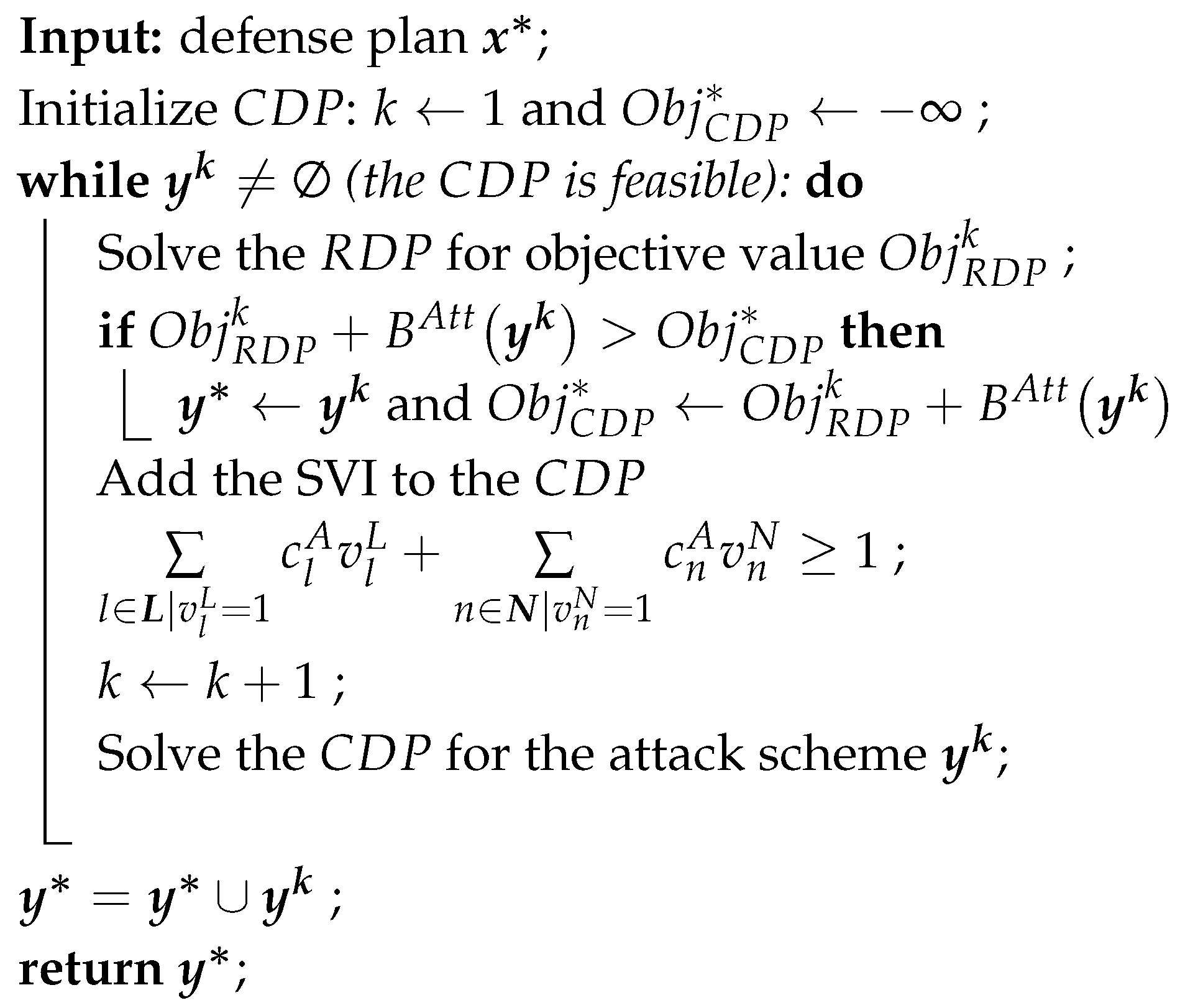
[25]	wind power photovoltaic power	DRO	Benders decomposition

compares the key features of resilience enhancement models in different literature.

To improve the resilience of the system to withstand extreme damage, this paper proposes a defense resource allocation method based on a tri-level defender–attacker–defender model. This method can deploy defense resources to protect critical components before the grid suffers damage, to mitigate grid losses, and enhance resilience. Meanwhile, a distributionally robust optimization model is proposed to mitigate the uncertainty of repair time due to different damage intensities. The main contributions of this paper are summarized as follows:

$\left(1\right)$ A tri-level DAD optimization model is developed to consider the restoration process of the grid, so as to obtain the optimal deployment strategy of defense resources and enhance the system resilience.

$\left(2\right)$ A distributionally robust optimization (DRO) model is proposed to provide a robust solution to the resource allocation problem by considering the impact of repair time uncertainty on the return of the system to normal operation.

$\left(3\right)$ An algorithm combining the set covering method and column and constraint generation is developed to quickly solve the mixed integer model, and the optimal resource allocation plan is obtained by using the iterative relationship between the master problem and the subproblems.

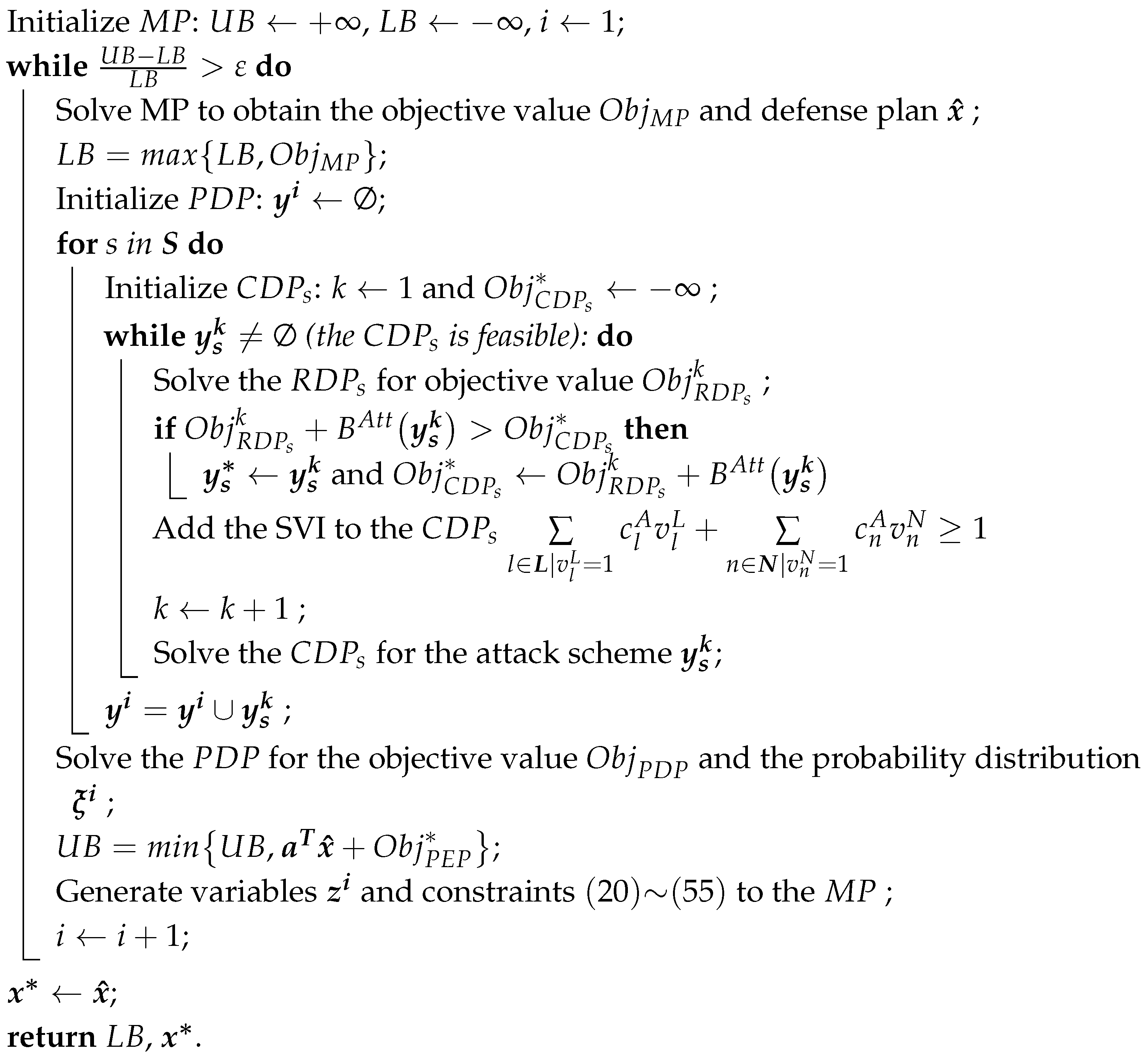
The rest of this paper is organized as follows. Section 2 describes the proposed TDR-DAD model in detail. Section 3 presents the SC-C&CG solution method. In order to verify the validity of the proposed model and solution method, Section 4 shows the case study and the corresponding results. Finally, Section 5 summarizes the work of this paper and future perspectives.

2. Problem Formulation

2.1. Overall System Framework

Uncertainty in the damage intensity is modelled using a Wasserstein distance-based DRO to strike a balance between robustness and conservativeness. The proposed resilience enhancement model adopts a tri-level DAD framework to address coordinated decision-making under extreme contingencies. This Stackelberg game-theoretic structure comprises three interdependent decision layers: (1) pre-event defense resource allocation, (2) worst-case attack identification, and (3) post-attack emergency recovery. The distinctive strength of the DAD framework lies in its ability to simultaneously optimize proactive hardening measures and reactive recovery strategies against extreme events.

In the first stage, defensive resources are pre-allocated to reinforce critical transmission lines and nodes, while MEGs and MTs are strategically positioned to ensure redundancy. The subsequent attacker layer solves the bilevel optimization problem to identify the most disruptive attack strategy that maximizes grid damage, considering both line outages and generator incapacitation. The final defender stage implements emergency response actions, where available MEGs and MTs are dispatched for rapid power supply restoration and repair crews are optimally routed to mitigate cascading failures and restore normal operations.

Notably, the recovery phase is specifically designed for contingency scenarios derived from the identified worst-case attack strategies. This formulation generates two critical outputs: (1) a robust allocation plan for reinforcing the deployment of resources, MEGs, and MTs and (2) a methodological framework guiding emergency repair operations. While the model prioritizes preventive defense strategies through min–max optimization, it intentionally excludes real-time repair scheduling from the decision variables to maintain computational tractability.

2.2. Uncertainty Modelling

Repair time is used to model the uncertainty in representing damage intensity. The greater the damage intensity, the longer the repair time. An ambiguity set is constructed to address the inherent uncertainty by using the Wasserstein distance metric. This approach enables the incorporation of all possible probability distributions while requiring only partial information about the underlying distribution. The proposed methodology determines the optimal reinforcement strategy by considering the worst-case probability distribution within the constructed ambiguity set, rather than relying on a predetermined distribution. This novel approach yields a more robust and realistic reinforcement strategy that is particularly suitable for power system applications.

Given two probability distributions $P_1$ and $P_2$, the Wasserstein distance is defined as the minimum transport cost to move $P_1$ to $P_2$ with minimum transport cost, with a general norm $∥·∥$. The formulation of the ambiguity set model is briefly described as follows.

$$\begin{array}{cc}\hfill d_W\left({\mathbb{P}}_1,{\mathbb{P}}_2\right)& =\underset{\mathbb{P}\in \mathcal{P}\left({\mathbb{P}}_1,{\mathbb{P}}_2\right)}{inf}{\mathbb{E}}_{\mathbb{P}}\left[∥{\tilde{\mathit{\xi }}}_{\mathbf{1}}-{\tilde{\mathit{\xi }}}_{\mathbf{2}}∥\right]\hfill \end{array}$$

(1)

$$\begin{array}{cc}\hfill \theta (N,\beta )& =S\sqrt{{\displaystyle \frac{2}{N}}ln{\displaystyle \frac{1}{1-\beta }}}\hfill \end{array}$$

(2)

S is the maximum Wasserstein distance between any pair of distributions in $\Gamma$. N is the number of historical data. $\beta$ is the confidence level for the distribution information. For any ${\tilde{\xi }}_1\sim {\mathbb{P}}_1$, ${\tilde{\xi }}_2\sim {\mathbb{P}}_1$, there is the cost of moving a Dirac point mass from ${\tilde{\xi }}_1$ to ${\tilde{\xi }}_2$, equal to $∥{\tilde{\xi }}_1-{\tilde{\xi }}_2∥$. $\mathcal{P}\left({\mathbb{P}}_1,{\mathbb{P}}_2\right)$ represents the set which contains all candidate joint contingency distributions. The distributionally robust ambiguity set $\Gamma \left(\theta \right)$, constructed to hedge against the uncertainty of disaster intensity, is defined as a Wasserstein ball encapsulating all probability distributions $\mathbb{P}$ within a prescribed radius $\theta \ge 0$ from an empirical reference distribution $\widehat{\mathbb{P}}$ (e.g., the empirical distribution derived from historical data). Mathematically,

$$\begin{array}{cc}\hfill & \Gamma \left(\theta \right)=\left\{\mathbb{P}\in \mathcal{P}\left({\mathbb{R}}^K\right)\left|\begin{array}{c}\left(\tilde{\mathit{\xi }}\right)\sim \mathbb{P}\hfill \\ d_W\left(\mathbb{P},\widehat{\mathbb{P}}\right)\le \theta \hfill \\ {\displaystyle \sum _{s\in S}}\mathit{\xi }=1\hfill \\ 0\le \mathit{\xi }\le 1\hfill \end{array}\right.\right\}\hfill \end{array}$$

(3)

The first term represents $\xi$ obeying a $\mathbb{P}$ distribution, the second term represents the true distribution being restricted to the Wasserstein radius $\theta$ of the empirical distribution, and the third and fourth terms represent $\xi$ being a positive distribution with a total probability of 1. $\theta$ controls the conservativeness of the model by regulating the deviation from the empirical distribution. The construction of ambiguity sets plays a key role in the development of system resilience enhancement scenarios. It covers all possible distributions of the repair time and finds the worst-case distribution from them to ensure that the defense scheme is effective in safeguarding the power supply when the system is damaged. This setup not only enhances the robustness of the system in the face of extreme disasters and deliberate attacks but also avoids the conservativeness of the scenarios developed by considering only the worst-case scenarios. Therefore, constructing an appropriate ambiguity set is crucial to resolving the uncertainty of the model parameters.

2.3. Objective Function

The proposed tri-level optimization framework aims to address the strategic inner dependencies between proactive grid hardening, adversarial attack selection, and adaptive recovery operations. Central to this formulation is a nested objective function that rigorously encodes the sequential decision-making logic of the DAD paradigm: defensive investments precede attack realization, which in turn governs post-event recovery efficacy. This structure ensures resilience planning which simultaneously optimizes preventive measures against worst-case disruptions while maintaining cost-effectiveness.

The objective function is structured hierarchically to reflect three critical operational dimensions: (1) Preventive Cost Minimization: Front-loaded investments in infrastructure hardening and mobile resource deployment; (2) Adversarial Risk Maximization: Explicitly quantifying the benefits of the attacker compromising critical components; and (3) Operational Resilience Maximization: Adaptive load shedding minimization under compromised grid conditions.

$$\begin{array}{c}\hfill \underset{\mathit{x}}{min}\left\{\begin{array}{c}{C}^{Def}+\\ \underset{{\mathbb{P}}_{RT}\in {\mathbf{\Gamma }}_{RT}}{max}\left[\underset{\mathit{y}}{max}\left(\begin{array}{c}{B}^{Att}+\\ \underset{\mathit{z}}{min}{L}^{Ls}+C^{Ope}\end{array}\right)\right]\end{array}\right\}\end{array}$$

(4)

where $\mathit{x}$, $\mathit{y}$, and $\mathit{z}$ are the decision variables for the three levels of optimization, respectively. ${\Gamma }_{AS}$ and ${\Gamma }_{RT}$ represent the distribution ambiguity sets for the number of attack resources and repair time, respectively, and $P_{AS}$ and $P_{RT}$ are the corresponding probability distributions. $C^{Def}$ is the defense resource cost. $B^{Att}$ is the benefit to the attacker from damaging the grid. $L^{Ls}$ and $C^{Ope}$ are the load-shedding loss and operation cost of the damaged grid.

2.3.1. First Layer Optimization

The objective function of the first level is to minimize the cost of defense, and the pertinent objective function and decision variables are as in Equations (5) and (6).

$$\begin{array}{cc}\hfill C^{Def}& =\sum _{l\in \mathit{L}}{c}_l^D{y}_l^L+\sum _{n\in \mathit{N}}{c}_n^D{y}_n^N\hfill \end{array}$$

(5)

$$\begin{array}{cc}\hfill \mathit{x}& =\left(y_l^L,y_n^N,w_{nn,0}^r,m_{nn,0}^k\right)\hfill \end{array}$$

(6)

where $\mathit{L}$ and $\mathit{N}$ are the set of lines and buses. $c_l^D$ and $c_n^D$ represent the cost required to defend the line l and node n, respectively. $y_l^L$ and $y_n^N$ are binary variables, equal to 1 for protecting the line l or the node n and 0 otherwise. $m_{nn,0}^k$ represents the initial deployment location of the MEG k, and $w_{nn,0}^r$ denotes the location of the MT r. It is worth noting that this will create discrete feasible regions, leading to non-convexity in the strategy space.

2.3.2. Second Layer Optimization

The objective of the second layer of the optimization model is to find the most destructive attack scenario in the constructed set of distributional ambiguities. The specific objective function and decision variables are elaborated in Equations (7) and (8).

$$\begin{array}{cc}\hfill B^{Att}& =\sum _{l\in \mathit{L}}{\omega }_l^A{v}_l^L+\sum _{n\in \mathit{N}}{\omega }_n^A{v}_n^N\hfill \end{array}$$

(7)

$$\begin{array}{cc}\hfill \mathit{y}& =\left(v_l^L,v_n^N\right)\hfill \end{array}$$

(8)

where ${\omega }_l^A$ and ${\omega }_n^A$ represent the destruction priority, the value of which is determined by the actual importance of each node or line. $v_l^L$ and $v_n^N$ are binary variables, equal to 1 for attacking the line l or the node n and 0 otherwise.

2.3.3. Third Layer Optimization

The purpose of the third layer is to minimize the total load-shedding loss caused by the damage before the grid returns to normal operation, following the determination of the defense scheme and damage strategy in the first two layers, respectively. Equations (9)–(11) show the details of the objective function and decision variables.

$$\begin{array}{cc}\hfill L^{Ls}& =\sum _{n\in \mathit{N}}\sum _{t\in \mathit{T}}{c}_n^{LS}{p}_{n,t}^{LS}\hfill \end{array}$$

(9)

$$\begin{array}{c}\hfill \begin{array}{cc}\hfill C^{Ope}& =\sum _{r\in R}\sum _{t\in \mathit{T}}\sum _{n,m\in N}{c}_r^{MT}{w}_{nm,t}^r\hfill \\ \hfill & +\sum _{k\in K}\sum _{t\in \mathit{T}}\sum _{n\in N}{c}_k^{MEG}{m}_{nn,t}^k\hfill \end{array}\end{array}$$

(10)

$$\begin{array}{cc}\hfill \mathit{z}& =\left(\begin{array}{c}{\alpha }_l^L,{\alpha }_n^N,{\beta }_{l,t}^L,{\beta }_{n,t}^N,\hfill \\ w_{nm,t}^r,w_{nn,t}^r,m_{nn,t}^k,p_{n,t}^{MEG},\hfill \\ p_{l,t}^L,p_{n,t}^G,p_{n,t}^{LS},{\delta }_{n,t}\hfill \end{array}\right)\hfill \end{array}$$

(11)

where $\mathit{T}$ is the time set. $c_n^{LS}$ represents the coefficient of the load-shedding loss. $c_r^{MT}$ and $c_k^{MEG}$ are the operation costs of the MT and MEG. $p_{n,t}^{LS}$ is the load shedding after the restoration phase. ${\alpha }_l^L$, ${\alpha }_n^N$, ${\beta }_{l,t}^L$, ${\beta }_{n,t}^N$, $w_{nm,t}^r$, $w_{nn,t}^r$, and $m_{n,t}^k$ are binary variables. ${\alpha }_l^L$ and ${\alpha }_n^N$ are equal to 0, indicating that the line l or node n is disconnected during the sabotage operation, and 1 otherwise. ${\beta }_{l,t}^L$ and ${\beta }_{n,t}^N$ are equal to 1, meaning that the line l or node n is reactivated at time t. $w_{nm,t}^r$ and $w_{nn,t}^r$ are the trajectories of the repair team recorded with the matrix. When it stops at the damaged components (equal to 1), it can be considered to repair the component. $m_{n,t}^k$ equals 1 denotes that MEG is powering node n at time t. $p_{n,t}^{MEG}$ and $p_{n,t}^G$ are the generated power of MEG and generator at node n at time t. $p_{l,t}^L$ is the power flow on line l at time t. $p_{n,t}^{LS}$ represents the load shedding at node n at time t. ${\delta }_{n,t}$ denotes the phase angle at node n at time t.

By integrating these components through a min–max–min operator sequence, the model captures the inherent asymmetry among defensive preparedness, attack, and restoration actions. The mathematical nesting ensures defensive strategies are evaluated against their effectiveness in limiting both direct attack impacts and subsequent restoration challenges, thereby aligning theoretical robustness with practical grid operational requirements.

2.4. Constraints

The constraint structure must systematically bridge expected hardening measures, disruption scenarios, and recovery countermeasures while explicitly addressing the inherent uncertainty: attack intensity constraints (as reflected in the time to repair components). The uncertainties propagate in both directions in the decision hierarchy—pre-event defenses change the attacker’s decision space, while post-event maintenance scheduling influences the formulation of defenses. To realize this interdependence, we construct constraints through three mutually recursive levels: (1) pre-disaster defense resource allocation under budget constraints, (2) adversarial attack selection considering limited attack resources and attack benefits, and (3) post-disaster restoration coordination integrating grid current balancing, MEG scheduling, and MT scheduling. It is worth noting that in constructing the constraints of the model, the big-M method is used to linearize the possible nonlinear terms, where M denotes a large constant.

2.4.1. First-Layer Constraints

The deployment of protection resources is an important part of system resilience enhancement, and by hardening some of the lines and nodes, the impact of extreme disasters and deliberate attacks can be effectively resisted. Specific constraints on the deployment of the defense resources are detailed below:

$$\sum _{l\in \mathit{L}}{c}_l^D{y}_l^L+\sum _{n\in \mathit{N}}{c}_n^D{y}_n^N\le B_D$$

(12)

$$\begin{array}{cc}\hfill & \sum _{r\in R}\sum _{n\in N}{w}_{nn,0}^r\le R\hfill \end{array}$$

(13)

$$\begin{array}{cc}\hfill & \sum _{k\in K}\sum _{n\in N}{m}_{nn,0}^k\le K\hfill \end{array}$$

(14)

$$\begin{array}{cc}\hfill & y_l^L\in \left\{0,1\right\},\forall l\in \mathit{L}\hfill \end{array}$$

(15)

$$\begin{array}{cc}\hfill & y_n^N\in \left\{0,1\right\},\forall n\in \mathit{N}\hfill \end{array}$$

(16)

$B_D$ is the defense resource budget. R and K are the number of MTs and MEGs. Constraint (12) represents the budgetary constraints on the investment of total defense resources. Constraints (13) and (14) limit the initial number of MT and MEG deployments.

2.4.2. Section-Layer Constraints

The second layer involves identifying the optimal disruption strategies under different attack resource scenarios for the attacker. Disrupting some of the lines and nodes in the grid can cause maximum load shedding during grid operation. The specific constraints are as follows:

$$\sum _{l\in \mathit{L}}{c}_l^A{v}_l^L+\sum _{n\in \mathit{N}}{c}_n^A{v}_n^N\le B_A$$

(17)

$$\begin{array}{cc}\hfill & v_l^L\in \left\{0,1\right\},\forall l\in \mathit{L}\hfill \end{array}$$

(18)

$$\begin{array}{cc}\hfill & v_n^N\in \left\{0,1\right\},\forall n\in \mathit{N}\hfill \end{array}$$

(19)

$B_A$ is the attack resource budget. Constraint (17) means that the maximum number of destroyed components cannot exceed the attack budget.

2.4.3. Third-Layer Constraints

The third layer focuses on constraints on the dispatch of restorative resources and the generation power regulation. Constraints (20)–(55) provide a full breakdown of the model construction.

$\left(1\right)$ Component state constraints:

$$\begin{array}{cc}\hfill & v_l^L\left(y_l^L-1\right)+1={\alpha }_l^L,\forall l\in \mathit{L}\hfill \end{array}$$

(20)

$$\begin{array}{cc}\hfill & v_n^N\left(y_n^N-1\right)+1={\alpha }_n^N,\forall n\in \mathit{N}\hfill \end{array}$$

(21)

$$\begin{array}{cc}\hfill & {\alpha }_l^L\le 1-{\beta }_{l,t}^L,\forall l\in \mathit{L},t\in \mathit{T}\hfill \end{array}$$

(22)

$$\begin{array}{cc}\hfill & {\alpha }_n^N\le 1-{\beta }_{n,t}^N,\forall n\in \mathit{N},t\in \mathit{T}\hfill \end{array}$$

(23)

$$\begin{array}{cc}\hfill & {\beta }_{l,1}^L=0,\forall l\in \mathit{L}\hfill \end{array}$$

(24)

$$\begin{array}{cc}\hfill & {\beta }_{n,1}^N=0,\forall n\in \mathit{N}\hfill \end{array}$$

(25)

Constraints (20) and (21) represent the state of the line or node. Constraints (22) and (23) indicate whether the damaged components are repaired at time t. Constraints (24) and (25) emphasize that the disconnected nodes and lines will not be repaired until the next time.

$\left(2\right)$ MT dispatching constraints:

$$\begin{array}{cc}\hfill & \sum _{nm\in {\mathit{L}}_{+}^{\mathit{r}}}{w}_{nm,t+1}^r-\sum _{nm\in L_{-}^r}{w}_{nm,t}^r=0,\forall t\in \mathit{T},\forall r\in \mathit{R}\hfill \end{array}$$

(26)

$$\begin{array}{cc}\hfill & \sum _{nm\in {\mathit{L}}_{+}^{\mathit{r}}}{w}_{nm,1}^r-w_{nm,0}^r=0,\forall nm\in \mathit{L},\forall r\in \mathit{R}\hfill \end{array}$$

(27)

$$\begin{array}{cc}\hfill & w_{nm,T}^r-\sum _{nm\in L_{-}^r}{w}_{nm,T}^r=0,\forall nm\in \mathit{L}\hfill \end{array}$$

(28)

$$\begin{array}{c}\hfill \begin{array}{cc}\hfill & \sum _{s=1}^t{w}_{nm,s}^r\le M\left(1-\left(w_{nm,t+1}^r-w_{nm,t}^r\right)\right),\hfill \\ \hfill & \forall nm\in \mathit{L},\forall t\in \mathit{T},\forall r\in \mathit{R}\hfill \end{array}\end{array}$$

(29)

$$\begin{array}{c}\hfill \begin{array}{cc}\hfill & \sum _{s=1}^t{w}_{nn,s}^r\le M\left(1-\left(w_{nn,t+1}^r-w_{nn,t}^r\right)\right),\hfill \\ \hfill & \forall n\in \mathit{N},\forall t\in \mathit{T},\forall r\in \mathit{R}\hfill \end{array}\end{array}$$

(30)

$$\begin{array}{cc}\hfill & \sum _{s\in \mathit{R}|s=r}\sum _{t\in \mathit{T}}{w}_{nm,t}^s\le M\left(1-w_{nm,t}^r\right),\forall nm\in \mathit{L},\forall r\in \mathit{R}\hfill \end{array}$$

(31)

$$\begin{array}{cc}\hfill & \sum _{s\in \mathit{R}|s=r}\sum _{t\in \mathit{T}}{w}_{nn,t}^s\le M\left(1-w_{nn,t}^r\right),\forall n\in \mathit{N},\forall r\in \mathit{R}\hfill \end{array}$$

(32)

$$\begin{array}{cc}\hfill & \sum _{r\in \mathit{R}}{w}_{nm,t}^r\le 1,\forall nm\in \mathit{L},\forall t\in \mathit{T}\hfill \end{array}$$

(33)

$$\begin{array}{cc}\hfill & \sum _{r\in \mathit{R}}{w}_{nn,t}^r\le 1,\forall n\in \mathit{N},\forall t\in \mathit{T}\hfill \end{array}$$

(34)

$$\begin{array}{cc}\hfill & \sum _{nm\in \mathit{L}}{w}_{nm,t}^r+\sum _{n\in \mathit{N}}{w}_{nn,t}^r=1,\forall r\in \mathit{R},\forall t\in \mathit{T}\hfill \end{array}$$

(35)

$$\begin{array}{cc}\hfill & \sum _{r\in \mathit{R}}\sum _{t\in \mathit{T}}{w}_{nm,t}^r\ge \left(1-{\alpha }_l^L\right)r{t}_l^L,\forall nm\in \mathit{L}\hfill \end{array}$$

(36)

$$\begin{array}{cc}\hfill & \sum _{t\in \mathit{T}}{w}_{nm,t}^r\ge T{r}_l^{L,r},\forall nm\in \mathit{L},\forall rin\mathit{R}\hfill \end{array}$$

(37)

$$\begin{array}{cc}\hfill & \sum _{r\in \mathit{R}}\sum _{t\in \mathit{T}}{w}_{nn,t}^r\ge \left(1-{\alpha }_n^N\right)r{t}_n^N,\forall n\in \mathit{N}\hfill \end{array}$$

(38)

$$\begin{array}{cc}\hfill & {\beta }_{l,t}^L\le {\displaystyle \frac{{\displaystyle \sum _{r\in R}}{\displaystyle \sum _{s=1}^{t-1}}{w}_{nm,s}^r}{\left(1-{\alpha }_l^L\right)r{t}_l^L}},\forall l\in \mathit{L}\hfill \end{array}$$

(39)

$$\begin{array}{cc}\hfill & {\beta }_{n,t}^N\le {\displaystyle \frac{{\displaystyle \sum _{r\in R}}{\displaystyle \sum _{s=1}^{t-1}}{w}_{nn,s}^r}{\left(1-{\alpha }_n^N\right)r{t}_n^N}},\forall n\in \mathit{N}\hfill \end{array}$$

(40)

Since the matrix facilitates the recording of trajectories, $nm$ is used instead of the line l with start point n and end point m. R is the MT set. ${\mathit{L}}_{+}$ and ${\mathit{L}}_{-}$ represent the set of routes for each MT and MEG, which are derived from the Dijkstra algorithm. $T{r}_l^{L,r}$ is the travel time on line l for MT r. M in constraints (29)–(55) denotes a good constant. Constraints (26)–(28) indicate trip coherence, i.e., the MTs can only drive into the adjacent roadway at the next moment. Constraints (29) and (30) show that maintenance tasks cannot be interrupted. Constraints (31) and (32) show that once an MT starts work, it must be completed before the next component is repaired. Constraints (33)–(35) limits repairs to one team per destroyed component and one component per team per repair. Constraints (36)–(38) represent the amount of time the MT has to work to ensure that the component is returned to normal, while $r{t}_l^L$ and $r{t}_n^N$ represent the amount of time required to repair the damaged component. Constraints (39) and (40) denote the time required to bring the component back to normal. The product of binary variables $w_{nn,s}^r$, $w_{nm,s}^r$, ${\alpha }_l^L$ and ${\alpha }_n^N$ introduce nonlinear, non-convex terms.

$\left(3\right)$ MEG operating constraints:

$$\begin{array}{cc}\hfill & \sum _{nm\in {\mathit{L}}_{+}^{\mathit{k}}}{m}_{nm,t+1}^k-\sum _{nm\in L_{-}^k}{m}_{nm,t}^k=0,\forall t\in \mathit{T},\forall k\in \mathit{K}\hfill \end{array}$$

(41)

$$\begin{array}{cc}\hfill & \sum _{nm\in {\mathit{L}}_{+}^{\mathit{k}}}{m}_{nm,1}^k-m_{nm,0}^k=0,\forall nm\in \mathit{L},\forall k\in \mathit{K}\hfill \end{array}$$

(42)

$$\begin{array}{cc}\hfill & m_{nm,T}^k-\sum _{nm\in L_{-}^k}{m}_{nm,T}^k=0,\forall nm\in \mathit{L}\hfill \end{array}$$

(43)

$$\begin{array}{cc}\hfill & \sum _{k\in \mathit{K}}{m}_{nm,t}^k\le 1,\forall nm\in \mathit{L},\forall t\in \mathit{T}\hfill \end{array}$$

(44)

$$\begin{array}{cc}\hfill & \sum _{k\in \mathit{K}}{m}_{nn,t}^k\le 1,\forall n\in \mathit{N},\forall t\in \mathit{T}\hfill \end{array}$$

(45)

$$\begin{array}{cc}\hfill & \sum _{nm\in \mathit{L}}{m}_{nm,t}^k+\sum _{n\in \mathit{N}}{m}_{nn,t}^k=1,\forall k\in \mathit{K},\forall t\in \mathit{T}\hfill \end{array}$$

(46)

$$\begin{array}{cc}\hfill & \sum _{t\in \mathit{T}}{m}_{nm,t}^k\ge T{r}_l^{L,k},\forall nm\in \mathit{L},\forall k\in \mathit{K}\hfill \end{array}$$

(47)

$$\begin{array}{c}\hfill \begin{array}{cc}\hfill & \sum _{s=1}^t{m}_{nn,s}^k\le M\left(1-\left(m_{nn,t+1}^k-m_{nn,t}^k\right)\right),\hfill \\ \hfill & \forall n\in \mathit{N},\forall t\in \mathit{T},\forall k\in \mathit{K}\hfill \end{array}\end{array}$$

(48)

$$\begin{array}{cc}\hfill & 0\le p_{n,t}^{MEG}\le \sum _{k\in \mathit{K}}{m}_{nn,t}^k{P}^{MEG},\forall n\in \mathit{N}\hfill \end{array}$$

(49)

K is the set of MEGs. Constraints (41)–(43) indicate trip coherence, i.e., the MEG can only drive into the adjacent roadway at the next moment. Constraints (44)–(46) specify a maximum of one MEG per bus. Constraint (47) emphasizes the journey dispatch time of the MEGs. $T{r}_l^{L,k}$ is the travel time on line l for MEG k. Constraint (48) shows that the power supply to the MEG cannot be interrupted unless component maintenance is completed. Constraint (49) limits the power generated by the MEG at node n.

$\left(4\right)$ Power balance constraints:

$$\begin{array}{c}\hfill \begin{array}{cc}\hfill & -\sum _{l\in \mathit{L}|o\left(l\right)=n}{p}_{l,t}^L+\sum _{l\in \mathit{L}|d\left(l\right)=n}{p}_{l,t}^L+p_{n,t}^{MEG}+p_{n,t}^G\hfill \\ \hfill & +p_{n,t}^{LS}=P_n^D,\forall n\in \mathit{N},\forall t\in \mathit{T}\hfill \end{array}\end{array}$$

(50)

$$\begin{array}{c}\hfill \begin{array}{cc}\hfill & -{\overline{P}}_l^L\left({\alpha }_l^L+{\beta }_{l,t}^L\right)\le p_{l,t}^L\hfill \\ \hfill & \le {\overline{P}}_l^L\left({\alpha }_l^L+{\beta }_{l,t}^L\right),\forall l\in \mathit{L},\forall t\in \mathit{T}\hfill \end{array}\end{array}$$

(51)

$$\begin{array}{c}\hfill \begin{array}{cc}\hfill & -{\overline{P}}_l^L\left({\alpha }_{o\left(l\right)}^N+{\beta }_{o\left(l\right),t}^N\right)\le p_{l,t}^L\hfill \\ \hfill & \le {\overline{P}}_l^L\left({\alpha }_{o\left(l\right)}^N+{\beta }_{o\left(l\right),t}^N\right),\forall l\in \mathit{L},\forall t\in \mathit{T}\hfill \end{array}\end{array}$$

(52)

$$\begin{array}{c}\hfill \begin{array}{cc}\hfill & -{\overline{P}}_l^L\left({\alpha }_{d\left(l\right)}^N+{\beta }_{d\left(l\right),t}^N\right)\le p_{l,t}^L\hfill \\ \hfill & \le {\overline{P}}_l^L\left({\alpha }_{d\left(l\right)}^N+{\beta }_{d\left(l\right),t}^N\right),\forall l\in \mathit{L},\forall t\in \mathit{T}\hfill \end{array}\end{array}$$

(53)

$$\begin{array}{cc}\hfill & 0\le p_{n,t}^G\le P_n^G\hfill \end{array}$$

(54)

$$\begin{array}{cc}\hfill & p_{l,t}^L{x}_l=\left({\alpha }_l^L+{\beta }_{l,t}^L\right)\left({\delta }_{o\left(l\right),t}-{\delta }_{d\left(l\right),t}\right),\forall l\in \mathit{L},\forall t\in \mathit{T}\hfill \end{array}$$

(55)

Constraint (50) ensures the power inflow and outflow balance at each bus n. $P_n^D$ denotes the load demand at bus n. Constraints (51)–(53) show the upper and lower limits associated with line and node states. Constraint (54) limits the power generation at bus n. Constraint (55) calculates the power flow on the transmission lines. The multiplicative term $\left({\alpha }_l^L+{\beta }_{l,t}^L\right)\left({\delta }_{o\left(l\right),t}-{\delta }_{d\left(l\right),t}\right)$ is bilinear, creating non-convexity.

3. Solution Method

The DAD model fundamentally captures the strategic interaction between two adversarial agents, the defender and the attacker. To resolve the computational complexity inherent in this nested structure, we employ a customized SC-C&CG algorithm that transforms the tri-level optimization model into a two-layer model containing the master problem (MP) and the subproblem (SP). In the MP, the defender determines the optimal allocation plan of defense resources based on the combination of attack strategies input from the SP, while the MP generates the lower bound of the proposed model. In the SP, the interaction between the attacker and the defender is modeled by a two-stage optimization problem in which the attacker decides the attack scheme that maximizes the grid load shedding, while the defender minimizes the load shedding by dispatching the restoration resource. The optimal attack solution obtained by the attacker among all the scenarios constitutes the attack strategy combinations. The two constructed problems are solved iteratively to narrow the gap between the two boundaries until satisfying predefined convergence criteria. The mathematical architecture of this decomposition framework will be elaborated subsequently.

3.1. Reformulation of the TDR-DAD Model

To simplify the exposition, the TDR-DAD model proposed in this paper is compactly represented in matrix form as follows.

$$\begin{array}{cc}\hfill & \underset{\mathit{x}}{min}\left\{{\mathit{a}}^{\mathit{T}}\mathit{x}+\underset{{\mathbb{P}}_{RT}\in {\mathbf{\Gamma }}_{RT}}{max}\left[\underset{\mathit{y}}{max}\left({\mathit{b}}^{\mathit{T}}\mathit{y}+\underset{\mathit{z}}{min}{\mathit{c}}^{\mathit{T}}\mathit{z}\right)\right]\right\}\hfill \end{array}$$

(56)

$$\begin{array}{c}\hfill \begin{array}{cc}\hfill & \mathrm{s}.\mathrm{t}.\mathit{Ax}+\mathit{By}+\mathit{Cz}\le \mathit{d},\mathit{Ex}\le \mathit{f},\mathit{Gy}\le \mathit{h},\hfill \\ \hfill & \mathit{Iz}\le \mathit{j},\mathit{K}{\mathbb{P}}_{RT}\le \mathit{l}\hfill \end{array}\end{array}$$

(57)

where $\mathit{a}$, $\mathit{b}$, and $\mathit{c}$ are the coefficient vector. $\mathit{A}$, $\mathit{B}$, $\mathit{C}$, $\mathit{E}$, $\mathit{G}$, $\mathit{I}$, $\mathit{K}$ are the coefficient matrices, and $\mathit{d}$, $\mathit{f}$, $\mathit{h}$, $\mathit{j}$, $\mathit{l}$ are the right-hand-side parameter vector of the proposed model. The first constraint set includes Constraints (20)∼(25), the second constraint set includes Equations (12)–(16), and Equations (17)–(19) represent the third constraint set. The fourth constraint set includes Equations (29)–(55). Equations (1) and (3) specify the fifth constraint.

3.2. Master Problem

A two-layer min–min MP can be obtained by fixing the probability distribution of the repair time and the attacker’s damage schemes in the original model, as shown in constraints (59) and (60). The defense resource allocation plan obtained by solving the MP will be used as input to the subproblem. Since the MP only considers a subset of all possible damage schemes of the attacker, it is a relaxed problem compared to the original problem and provides a lower bound value for the model.

$$\begin{array}{cc}\hfill & \underset{\mathit{x}}{min}\left({\mathit{a}}^{\mathit{T}}\mathit{x}+\alpha \right)\hfill \end{array}$$

(58)

$$\begin{array}{cc}\hfill \mathrm{s}.\mathrm{t}.& \alpha \ge E_{{\widehat{\mathbb{P}}}_{RT}^i}\left[{\mathit{b}}^{\mathit{T}}{\widehat{\mathit{y}}}^{\mathit{i}}+{\mathit{c}}^{\mathit{T}}{\mathit{z}}^{\mathit{i}}\right]\hfill \end{array}$$

(59)

$$\begin{array}{cc}\hfill & \mathit{Ax}+\mathit{B}{\widehat{\mathit{y}}}^{\mathit{i}}+{\mathit{Cz}}^{\mathit{l}}\le \mathit{d},\mathit{Ex}\le \mathit{f},{\mathit{Iz}}^{\mathit{l}}\le \mathit{j}\hfill \end{array}$$

(60)

${\widehat{\mathbb{P}}}_{RT}^i$ is the probability distribution of the repair time and $\widehat{y}$ represents the attack scenario. Both are determined from the SP. i represents the number of current iterations. As SP feeds the new repair time probability distribution ${\widehat{\mathbb{P}}}_{RT}^i$ and damage schemes ${\widehat{y}}^i$ into the MP, the MP will generate new decision variables $z^i$ and new constraints (20)–(55).

3.3. Subproblem

The SP can be constructed as a tri-level max–max–min formulation including the grid destruction behavior of the attacker and the repair resource scheduling behavior of the defender under various possible damage intensity scenarios, as shown in Constraints (61) and (62). The SP provides an upper bound for the model since it only considers a subset of all possible defense plans. Solving the SP can obtain the probability distributions of the uncertain parameters and the optimal damage scheme, which can then be fed back to the MP.

$$\begin{array}{cc}\hfill & \underset{{\mathbb{P}}_{RT}\in {\mathbf{\Gamma }}_{RT}}{max}\left[\underset{\mathit{y}}{max}\left({\mathit{b}}^{\mathit{T}}\mathit{y}+\underset{\mathit{z}}{min}{\mathit{c}}^{\mathit{T}}\mathit{z}\right)\right]\hfill \end{array}$$

(61)

$$\begin{array}{c}\hfill \begin{array}{cc}\hfill \mathrm{s}.\mathrm{t}.& \mathit{A}\widehat{\mathit{x}}+\mathit{By}+\mathit{Cz}\le \mathit{d},\mathit{Gy}\le \mathit{h},\hfill \\ \hfill & \mathit{Iz}\le \mathit{j},\mathit{K}{\mathbb{P}}_{RT}\le \mathit{l}\hfill \end{array}\end{array}$$

(62)

Since the proposed model is a complex mixed-integer optimization problem and can not satisfy the KKT condition, the max–min terms in the SP cannot be transformed into a single-level max optimization model through the strong duality theory. The SP is relaxed to a multi-scenario probability distribution combinatorial problem (PDP). It contains the component damage planning problem (CDP) and the repair resource dispatching problem (RDP) under different repair time scenarios and is efficiently solved by an improved ensemble covering algorithm. These problems are defined by the corresponding decision variables and are subject to the relevant constraints in the SP. The detailed model formulation and solution method are given below.

3.3.1. Probability Distribution Combination Problem (PDP)

The objective of PDP is to maximize the expected loss, which requires finding the worst probability distribution within the ambiguity set to effectively deal with the uncertainty of the repair time.

$$\begin{array}{cc}\hfill & \underset{{\mathbb{P}}_{RT}\in {\mathbf{\Gamma }}_{RT}}{max}{E}_{{\mathbb{P}}_{RT}}\left[{\mathit{b}}^{\mathit{T}}{\mathit{y}}^{*}+{\mathit{c}}^{\mathit{T}}{\mathit{z}}^{*}\right]\hfill \end{array}$$

(63)

$$\begin{array}{cc}\hfill & \mathrm{s}.\mathrm{t}.\mathit{K}{\mathbb{P}}_{\mathrm{RT}}\le \mathit{l}\hfill \end{array}$$

(64)

3.3.2. Component Damage Planning Problem (CDP)

CDP is defined as the problem of maximizing the number of components destroyed. It is more advantageous for the attacker to destroy unprotected components than to destroy all protected components, so weights are assigned to components preferentially.

$$\begin{array}{c}\hfill \begin{array}{cc}\hfill \underset{\mathit{y}}{max}& \left(L+N+1\right)\left(\sum _{l\in \mathit{L}|y_l^L=0}{\omega }_l^A{v}_l^L+\sum _{n\in \mathit{N}|y_n^N=0}{\omega }_n^A{v}_n^N\right)\hfill \\ \hfill & +\left(\sum _{l\in \mathit{L}|y_l^L=1}{\omega }_l^A{v}_l^L+\sum _{n\in \mathit{N}|y_n^N=1}{\omega }_n^A{v}_n^N\right)\hfill \end{array}\end{array}$$

(65)

$$\begin{array}{cc}\hfill & \mathrm{s}.\mathrm{t}.\mathit{Gy}\le \mathit{h}\hfill \end{array}$$

(66)

3.3.3. Repair Resource Dispatching Problem (RDP)

RDP is defined as the problem of minimizing grid load-shedding losses. Given the defense plan and the attack scheme, the defender minimizes the total load-shedding loss by dispatching restoration resources to return the grid to normal operation as soon as possible.

$$\begin{array}{cc}\hfill & \underset{\mathit{z}}{min}{\mathit{c}}^{\mathit{T}}\mathit{z}\hfill \end{array}$$

(67)

$$\begin{array}{cc}\hfill & \mathrm{s}.\mathrm{t}.\mathit{A}\widehat{\mathit{x}}+\mathit{B}\widehat{\mathit{y}}+\mathit{Cz}\le \mathit{d},\mathit{Iz}\le \mathit{j}\hfill \end{array}$$

(68)

3.3.4. Improved Set Covering Algorithm

The goal of the subproblem is to obtain the combination of the attacker’s damage strategies and the upper bound of the model. At each iteration, the CDP adds a constraint known as the SVI to find at least one unattacked component to narrow the feasible region and keeps updating the solution until the problem becomes infeasible and the algorithm terminates. The implementation steps of the algorithm are shown in Algorithm 1.

Algorithm 1: Improved set covering algorithm

As the number of candidate components increases, the number of possible combinations of attacked components also grows exponentially, leading to an increase in computational complexity. To address this problem, various different centroid metrics have been used in the literature to generate different sets of attack candidate components [29]. Aggregated hierarchical clustering techniques are used to generate sets representing a variety of different components, thus reducing the size of the problem. Due to space limitations, the load centrality is used to rank the nodes and select the highest ranked $25\%$ nodes for the experiments. The result has been verified in [5].

3.4. SC-C&CG Algorithm

The proposed tri-level model is decomposed into MP and SP and is solved iteratively using a customized SC-C&CG algorithm. The MP optimizes the defense plan using a combination of attack strategies imported from the SP and generates the lower bound ($LB$) on the model. The SP calculates the maximum load-shedding loss for all repair time scenarios and obtains the corresponding attack strategies. These attack strategies obtained for all scenarios constitute an attack strategy portfolio, which is added to the set of attack strategy portfolios if the model does not reach convergence. Then, it finds the worst probability distribution over the range of the ambiguity sets and calculates the expected load-shedding loss, which constitutes the upper bound ($UB$) of the model. The LB is non-decreasing, while UB is non-increasing, narrowing the gap until coverage. As shown in Algorithm 2. Since the attack and defense budgets are limited, the optimal solution is obtained by iteratively generating a new set of variables and constraints and solving the updated master problem, where eventually both the upper and lower bounds converge. $\epsilon$ is the given limit on the ratio of convergence, indicating the stopping criterion of the algorithm.

Algorithm 2: SC-C&CG algorithm

4. Case Study

To evaluate the effectiveness of the proposed tri-level distribution robust optimization model and the SC-C&CG algorithm, a case study is conducted on the modified IEEE 24-bus [30] test systems, which are mainly based on the topology of the distributed distribution network of these two systems operating as a mesh. Due to the broad range of the transmission network, the total simulation time is set to 14 days, with a unit time of 1 day. The maintenance time scenarios are set to [1, 2, 3, 4] days with the corresponding probability distributions of [0.40, 0.30, 0.20, 0.10] depending on the damage intensity. Experience distribution is obtained from historical data and can be adjusted according to different regional conditions. The power network structure used in this study is rigorously tested based on the Matpower software to ensure the authenticity of the results. The model is developed in MATLAB R2021b using the YALMIP toolbox and solved using the commercial solver GUROBI. Computational simulations are performed on a laptop equipped with an Intel Core i7-9750H CPU and 16 GB of RAM.

4.1. Experimental Setting

The power is uniformly set at kW. For the defender, the unit cost of protection of a line is USD 900/km, and the cost of protection of each line is obtained by multiplying its length by the unit cost. The cost of defending the bus is USD 100,000. For the attacker, the destruction priority of the line and bus is set to 1 and 2, respectively. The cost of breaking the line and the bus is USD 10,000 and USD 20,000, respectively. The cost of defending the line and bus is USD 15,000. The cost per unit of time for the load-shedding loss is USD 100/kW. The fuel cost of the MEG is USD 200/day. The defense budget is set to USD 30,000. The attack budget is set to USD 50,000. The destruction priority of the bus and the line is set to 2 and 1, respectively. The system is equipped with two 100 kW MEGs and two MTs. The MEG can only supply power to the buses in which they are located and cannot support the demands of the entire system through grid integration. Each bus has enough fuel to keep the MEG running until the system is repaired.

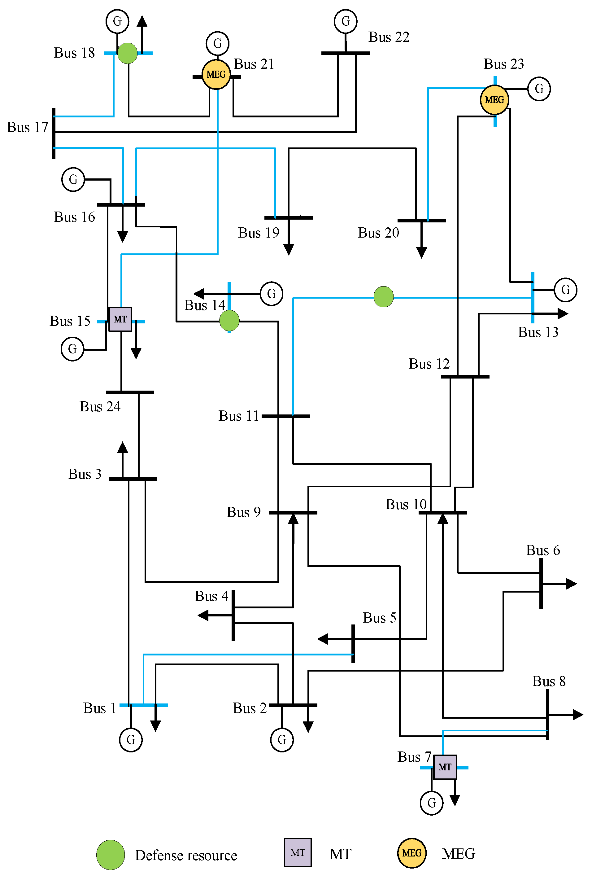
The modified 24-bus system consists of 11 generation buses, 17 load buses, and 34 lines. The system voltage is set to 10 kV to match the MEG dispatch, and the topology is shown in Figure 1. The top 25% of candidate nodes and line sets after screening by load centrality are marked in red.

4.2. Computational Results

The results calculated in the IEEE 24-bus system are shown in Figure 1, where the protection scheme includes line 11–13 and buses 14 and 18. The MEG is pre-deployed at buses 21 and 23, and the MT is pre-deployed at buses 7 and 15.

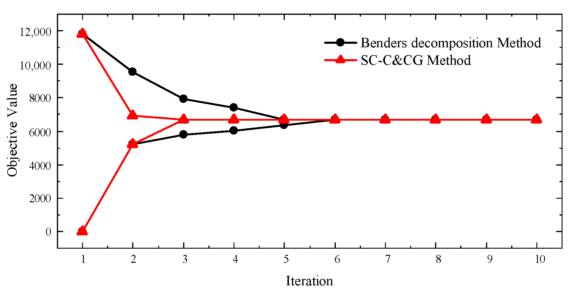
The model yielded results after only three iterations within 1462 s, and the convergence of the upper and lower bounds of the model is shown in Figure 2. The number of iterations using the Benders decomposition method is much greater than that of the proposed method, and the time required is 3274 s. The worst probability distribution in the constructed distribution ambiguity set is obtained as [0.4067, 0.3022, 0.1978, 0.0933].

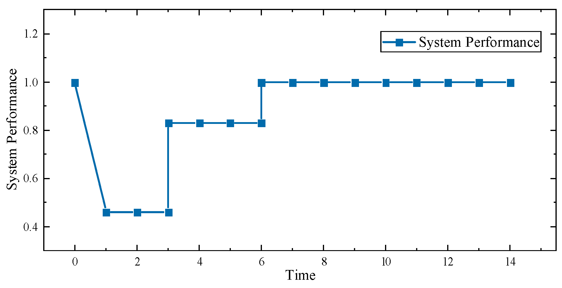
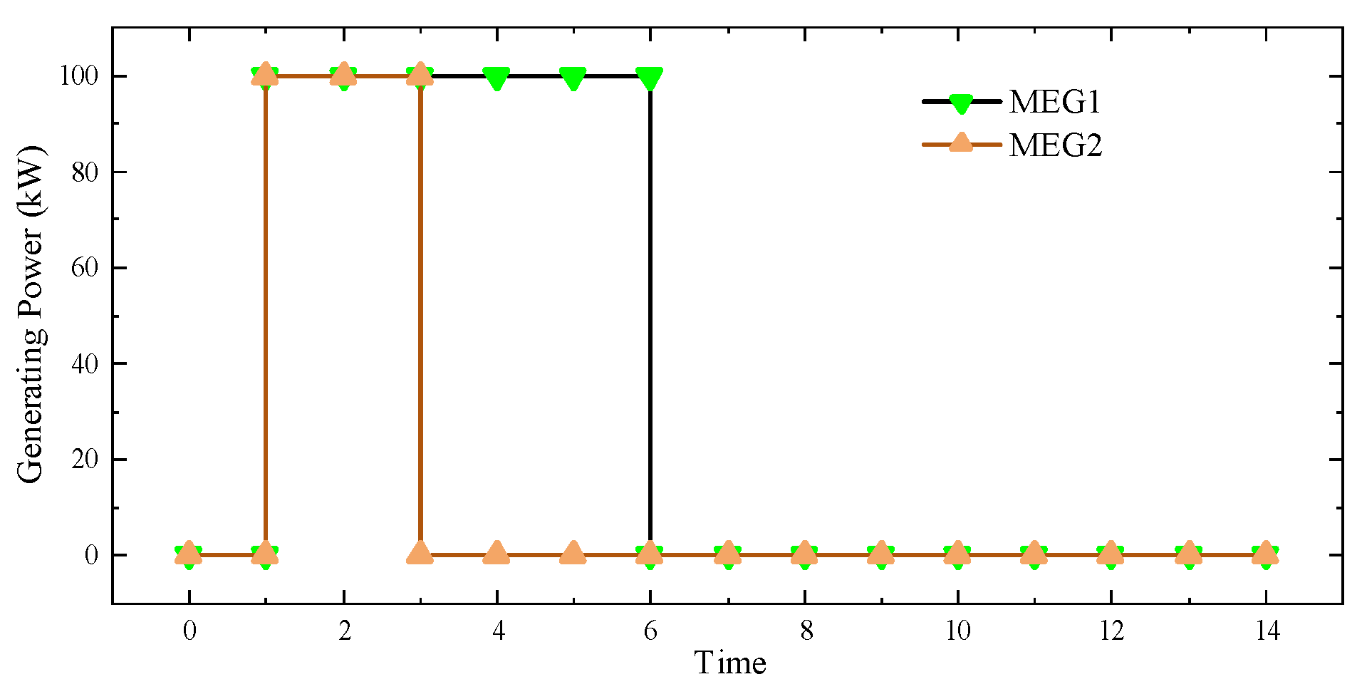
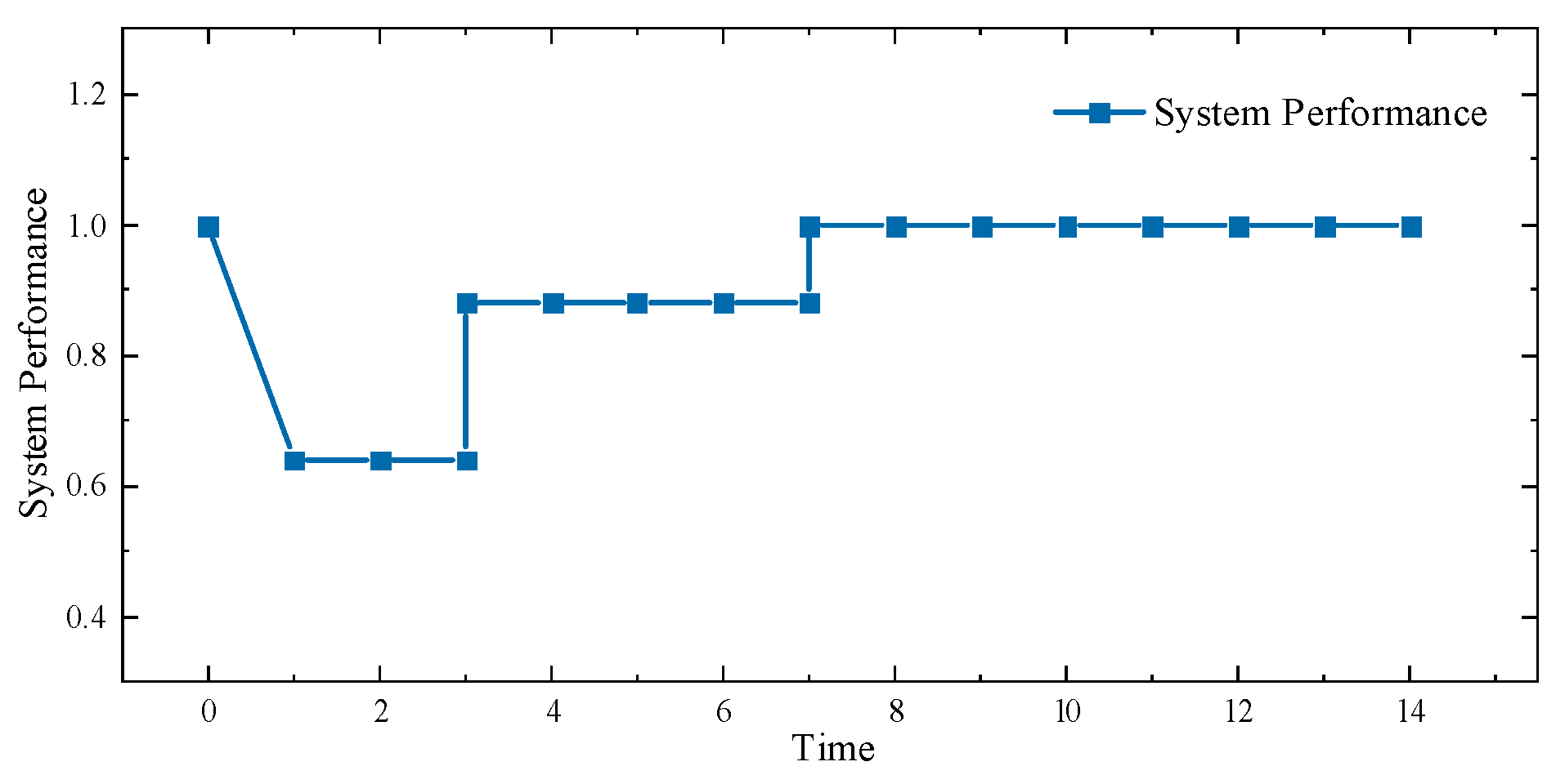
Figure 3 and Figure 4 show the status of the system during the two-day repair period. As shown in the figures, the system immediately began power adjustments and dispatched repair teams after the damage occurred. At time point 1, both MEGs began generating power, and MEG 2 stopped its emergency power supply on the third day, while MEG 1 continued to operate until the sixth day, at which point the entire system returned to normal. This is because MT takes one day to schedule damaged nodes and two days to repair them.

4.3. Comparison of Uncertainty Modeling Methods

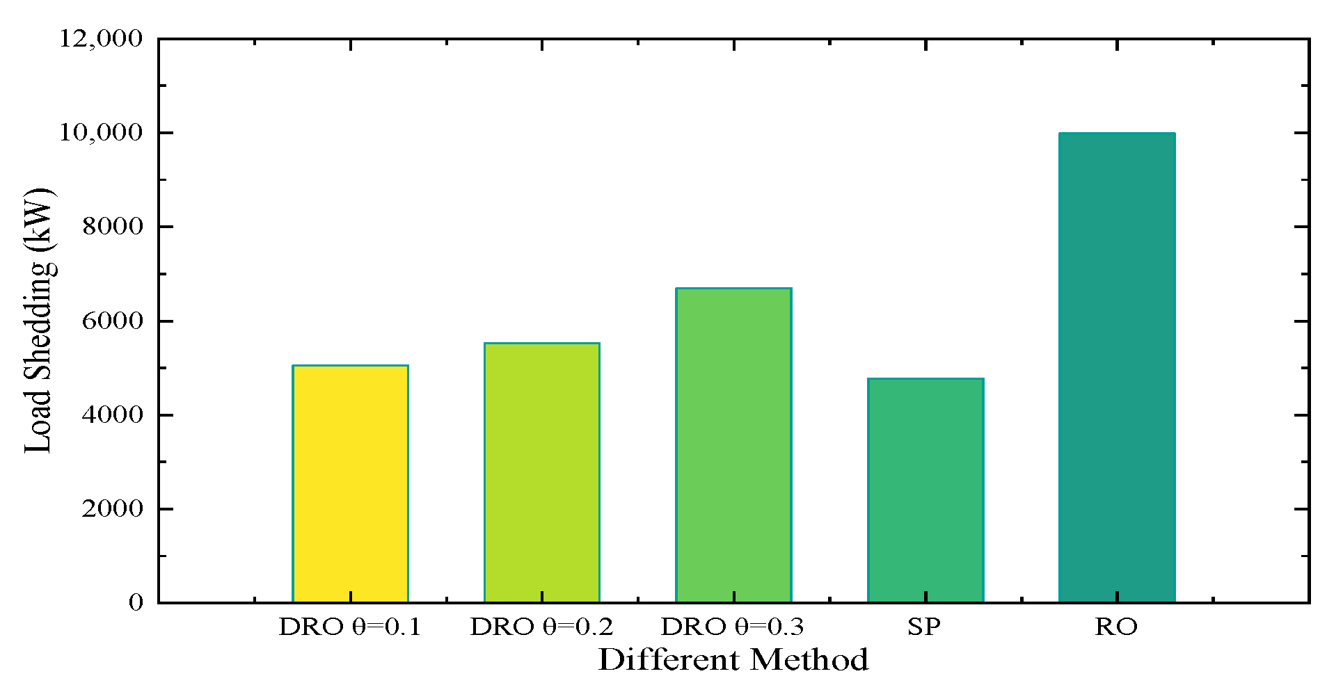
This section evaluates the utility of various methods for addressing repair time uncertainty. The main uncertainty modeling methods are SP, RO, and DRO. Given the repair time scenarios [1, 2, 3, 4] and the empirical distributions [0.4, 0.3, 0.2, 0.1], experimental comparisons are made in the case of the same defense and attack budget, and the results under the different methods are shown in Figure 5.

This figure clearly shows that RO yields the largest load-shedding loss because it considers all possible scenarios, resulting in an overly conservative solution. SP has the smallest load-shedding loss because the method solves only for a specific distribution. The value of DRO then shows a balanced solution that avoids being overly conservative and also avoids being overly dependent on the exact distribution of the information. This is because the DRO method makes full use of historical data to build the ambiguity set of distributions based on the empirical distribution, thus covering a wider range of distributions. This extension enhances the robustness of the solution. The robustness can also change as the radius of the Wasserstein sphere changes, which demonstrates the flexibility of the DRO method.

4.4. Comparison of the Number of Different Scheduling Resources

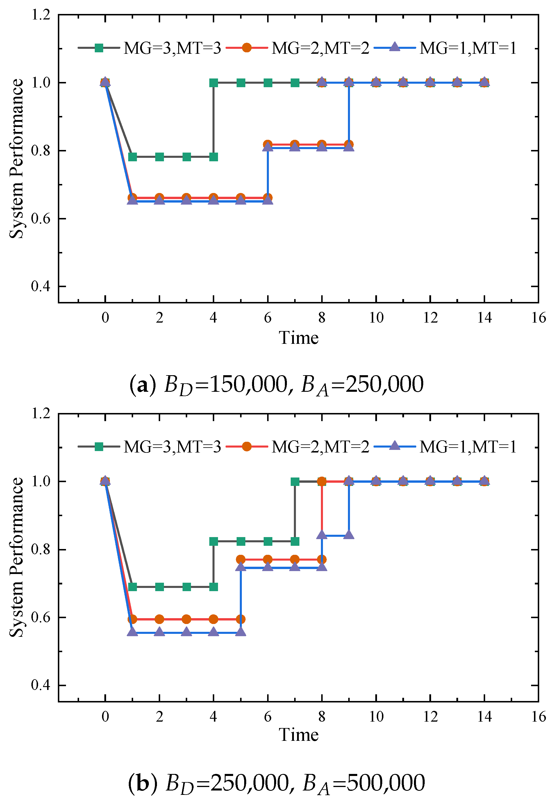
This section explores the impact of changes in the number of recovery resources on the system recovery process under different attack and defense budgets. Recovery resources are mainly the MEGs and MTs working in the recovery process. The purpose of this analysis is to investigate the effect of different numbers of recovery resources on the system recovery speed to ensure the consistency of the results. The budgets of defense and attack are set as [(150,000, 250,000), (250,000, 500,000)], and the combinations of MEGs and MTs are set as [(1,1), (2,2), (3,3)]. Multiple experiments are conducted based on the setup scenario, as shown in Figure 6.

This figure shows the recovery speed of the system for different scenarios. In the initial phase, the system suffers damage, and the load satisfaction rate decreases. Then, the defender starts dispatching MEGs and MTs until the whole system fully recovers. Obviously, using multiple MEGs and MTs can speed up the recovery process because multiple MTs can run in parallel, thus allowing the system to return to normal operation faster. From this figure, it can be seen that the greater the number of MEGs, the less the system performance degrades after damage. The higher the number of recovery resources, the faster the system returns to normal operation.

4.5. Effect Verification of the 118-Bus System

To assess the scalability of large-scale systems, the IEEE 118-bus system is used for validation. This larger system includes 118 buses, 186 transmission lines, 54 generation buses, and 99 load buses, providing a realistic scale for resilience studies. We set the same attack budget and defense budget, and conducted the test with a repair time of two days.

The changes in the load satisfaction rate of the power grid are shown in Figure 7. It can be seen that under the same budget, as the scale of the power grid increases, the impact of damage to the power grid decreases, but the larger mobility space also leads to longer recovery times.

5. Conclusions

In order to address the challenges posed by the uncertainty of damage intensity during grid resilience enhancement under extreme damage scenarios, a TDR-DAD model is proposed in this study. This model optimizes defense resource allocation, enhances maintenance resource scheduling, and generates distributional ambiguity sets using the Wasserstein distance to capture the probability distribution uncertainty of maintenance time. The main conclusions drawn from this study are that (1) the model can effectively handle the uncertainty of maintenance time when optimizing defense resource allocation, leading to a more resilient defense plan. The distributional ambiguity set based on Wasserstein distance does not require accurate and controllable information from historical data, but instead considers the main distribution information, thereby improving the robustness and accuracy of the model. (2) Compared with SO and RO, the DRO model realizes the balance of system economy and robustness, which verifies its effectiveness and superiority. In addition, the SC-C&CG algorithm significantly improves the computational efficiency while ensuring accuracy. The optimization results show that the more maintenance resources are invested, the more robust the system is. Furthermore, we recognize that the absence of a specific number of sabotage resources affects the formulation of defense costs and the optimization of defense schemes, which is a limitation of the current analysis. This limitation is due to the challenges posed by the asymmetry of attack and defense information. With the optimization of the uncertainty methodology and the availability of more data, future research will integrate these limitations, provide a more comprehensive analysis, and further validate the scheduling results. In the future, the challenges of integration with existing energy management systems (EMSs) and SCADA infrastructure will be a focus of research. In addition, studies will integrate climate projection models to optimize reinforcement strategies in the face of rising HILP event frequencies and develop dynamic ambiguity sets that evolve with climate-induced distribution shifts in repair times.