Author Contributions
Conceptualization, J.d.l.C.S., J.J.G.-A. and J.Y.R.-M.; data curation, G.O.-T., S.E.G.-C., H.M.B.-A., M.R.-M. and M.A.L.-O.; formal analysis, J.J.G.-A., J.Y.R.-M., J.P.-R. and O.A.V.-L.; investigation, M.A.Z.-G., F.D.J.S.-V., H.M.B.-A. and M.A.L.-O.; methodology, J.d.l.C.S., J.J.G.-A., M.A.Z.-G., J.P.-R. and O.A.V.-L.; software, S.E.G.-C. and M.R.-M.; validation, G.O.-T.; writing—original draft, J.J.G.-A.; writing—review and editing, J.Y.R.-M., G.O.-T., F.D.J.S.-V., S.E.G.-C., H.M.B.-A. and M.A.L.-O. All authors have read and agreed to the published version of the manuscript.
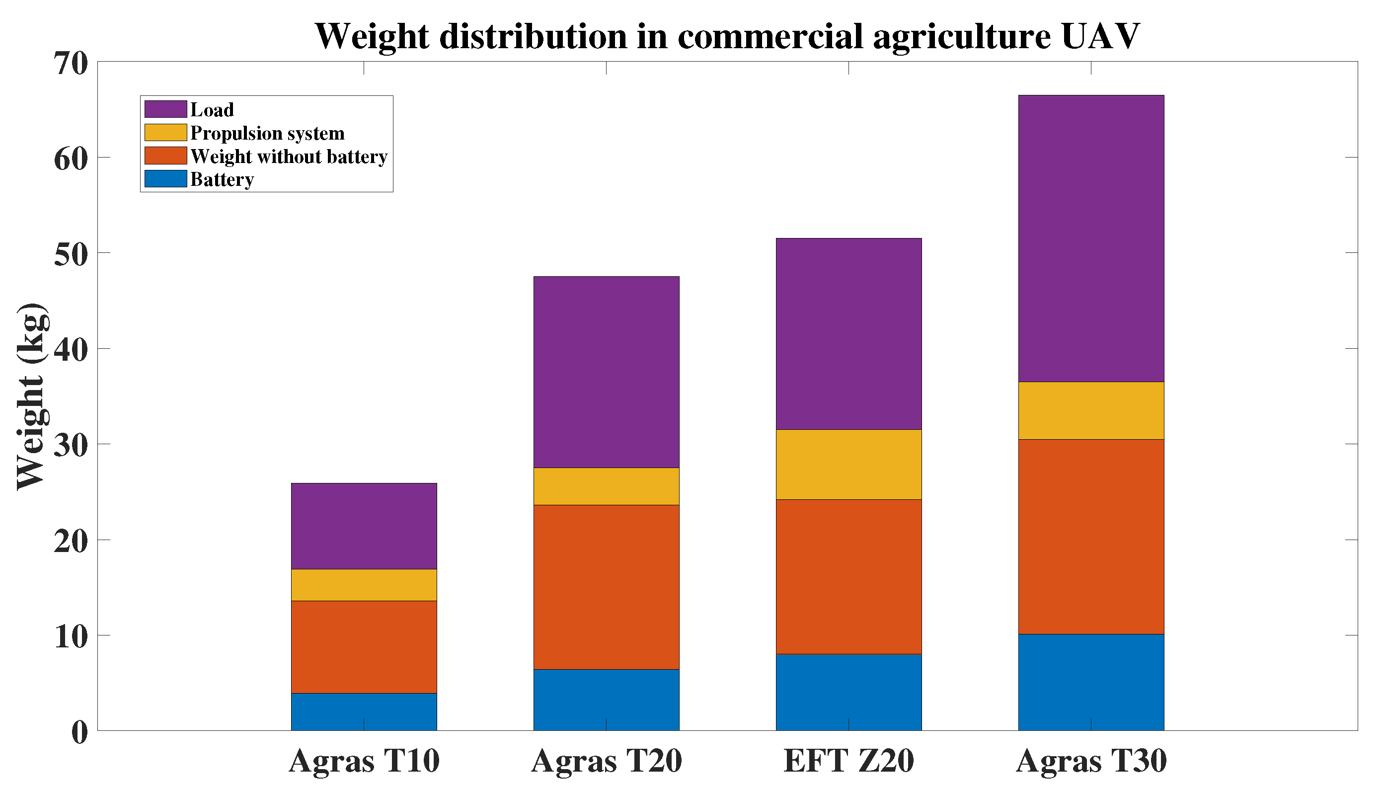
Figure 1.
Mass distribution in commercial agriculture UAVs.
Figure 1.
Mass distribution in commercial agriculture UAVs.
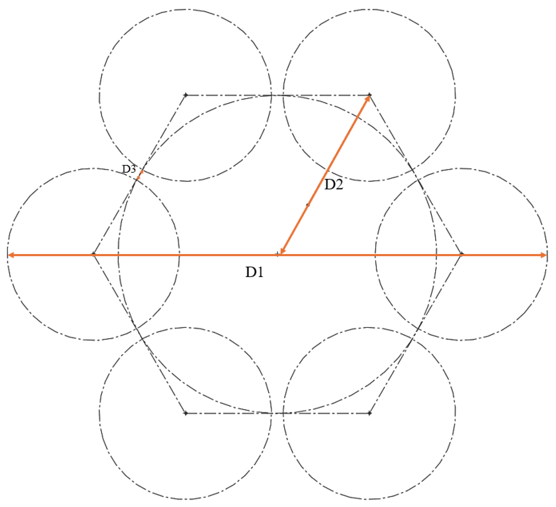
Figure 2.
Propeller and overall skeleton size characterization.
Figure 2.
Propeller and overall skeleton size characterization.
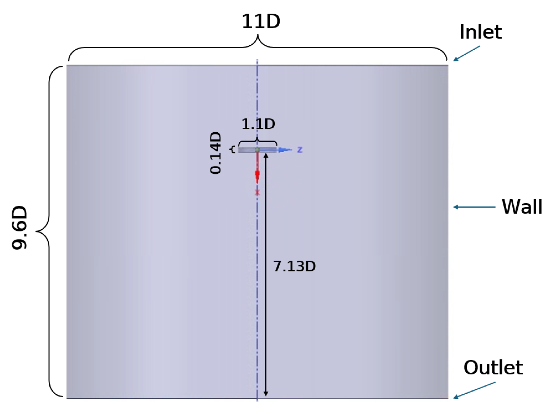
Figure 3.
Geometric characteristics of CFD domain.
Figure 3.
Geometric characteristics of CFD domain.
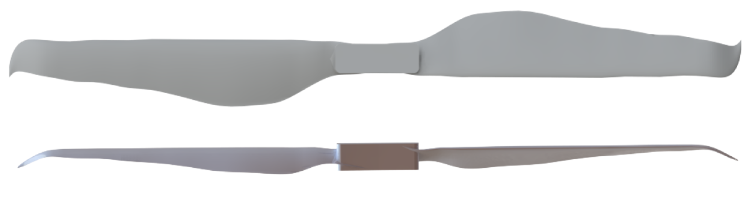
Figure 4.
Three-dimensional CAD design of 31.2 × 10.2 carbon fiber propeller.
Figure 4.
Three-dimensional CAD design of 31.2 × 10.2 carbon fiber propeller.
Figure 5.
Thrust–speed curve for the range of interest from CFD analysis.
Figure 5.
Thrust–speed curve for the range of interest from CFD analysis.
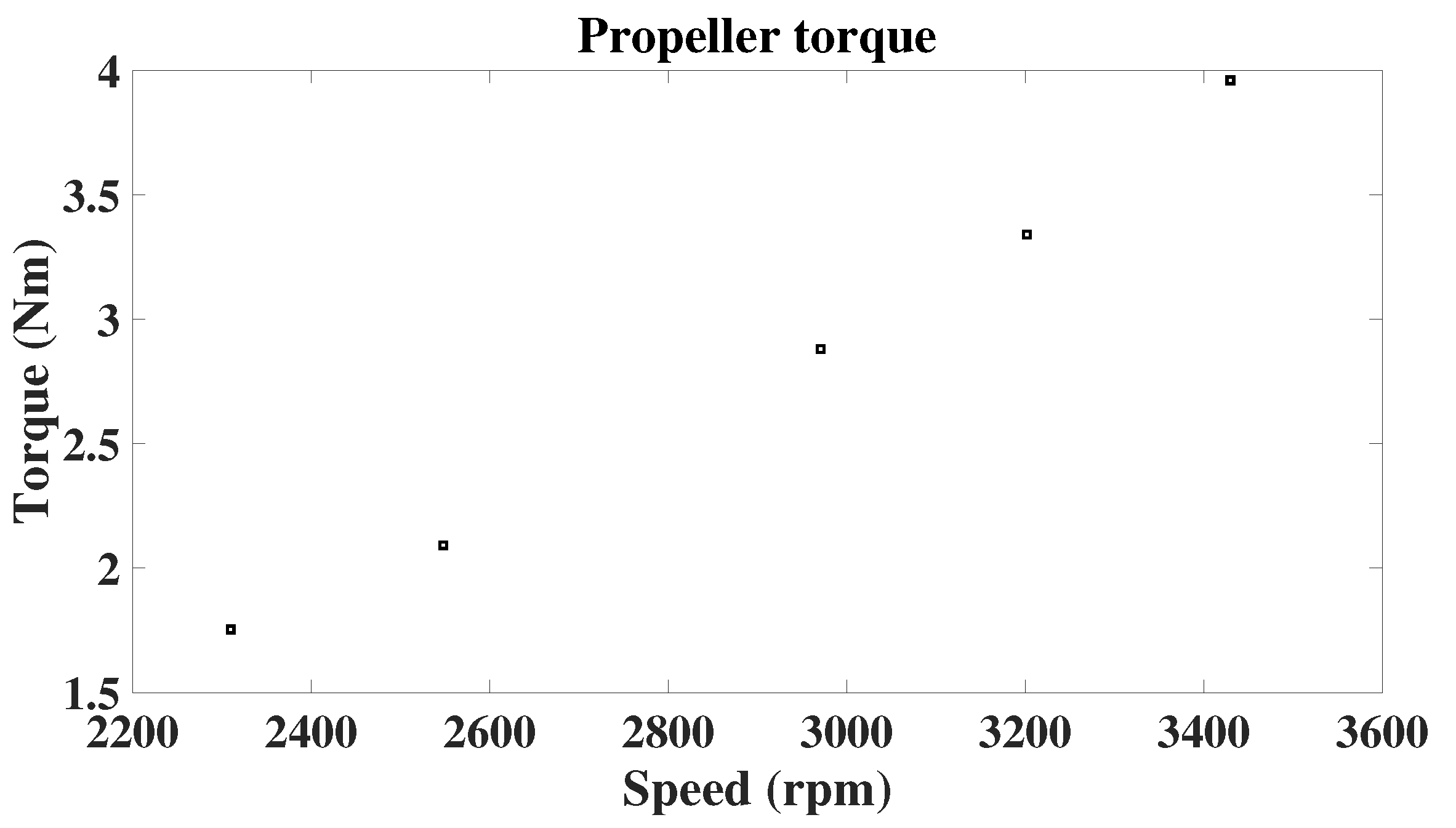
Figure 6.
Torque–speed curve for the range of interest from CFD analysis.
Figure 6.
Torque–speed curve for the range of interest from CFD analysis.
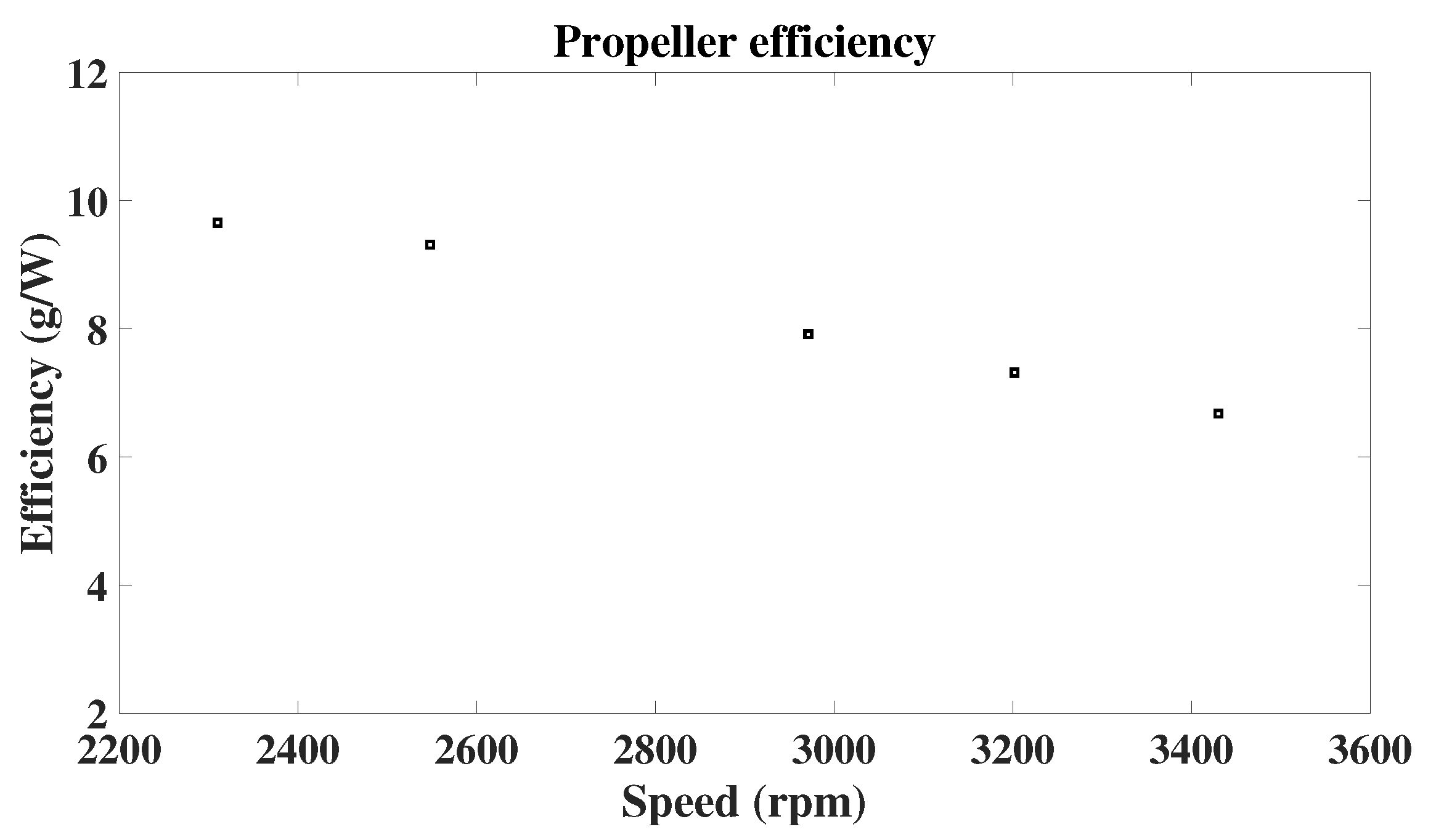
Figure 7.
Efficiency–speed curve for the range of interest from CFD analysis.
Figure 7.
Efficiency–speed curve for the range of interest from CFD analysis.
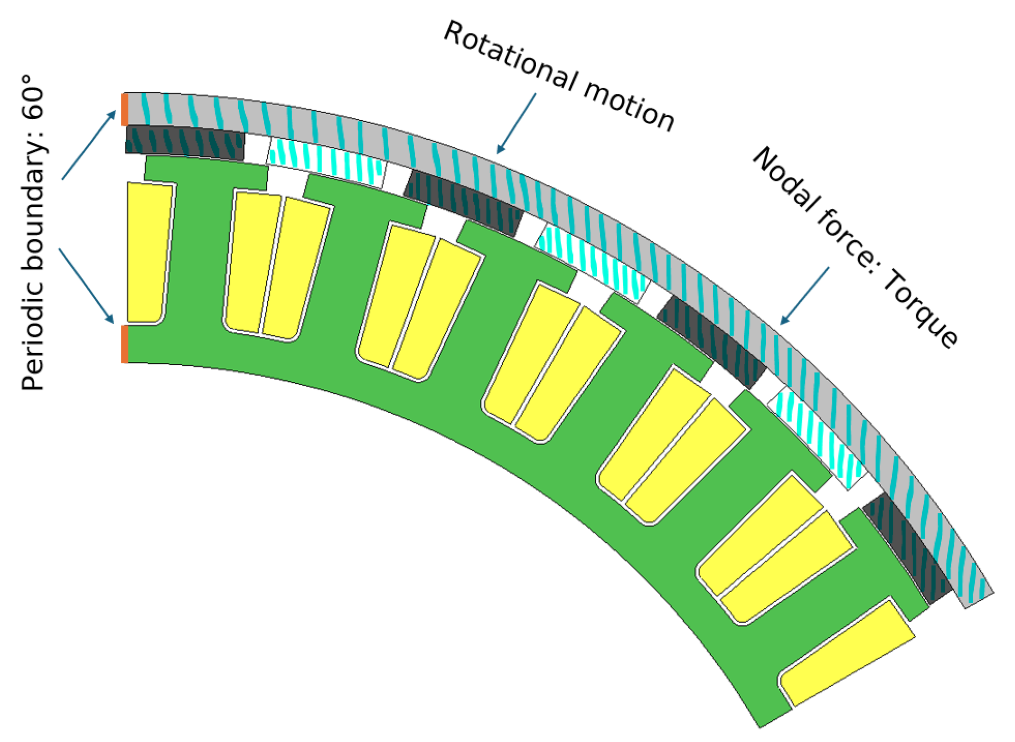
Figure 8.
Boundary conditions: electric motor simulation.
Figure 8.
Boundary conditions: electric motor simulation.
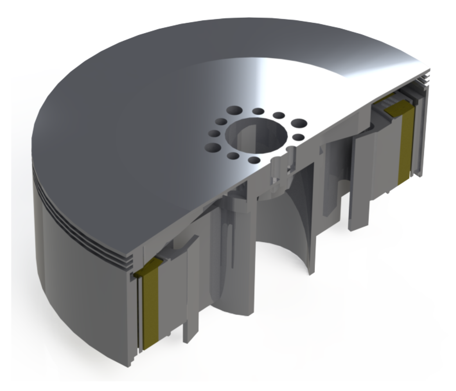
Figure 9.
Three-dimensional CAD U12II motor design.
Figure 9.
Three-dimensional CAD U12II motor design.
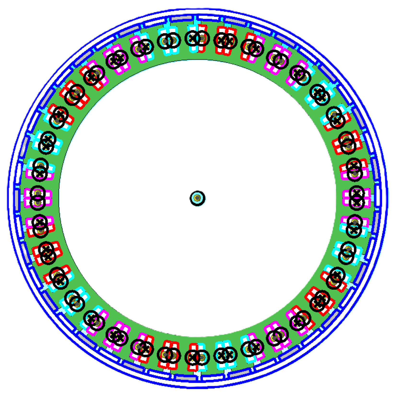
Figure 10.
U12II winding configuration.
Figure 10.
U12II winding configuration.
Figure 11.
Cogging torque in the U12II motor with 2548 rpm.
Figure 11.
Cogging torque in the U12II motor with 2548 rpm.
Figure 12.
Copper resistance evolution regarding source frequency.
Figure 12.
Copper resistance evolution regarding source frequency.
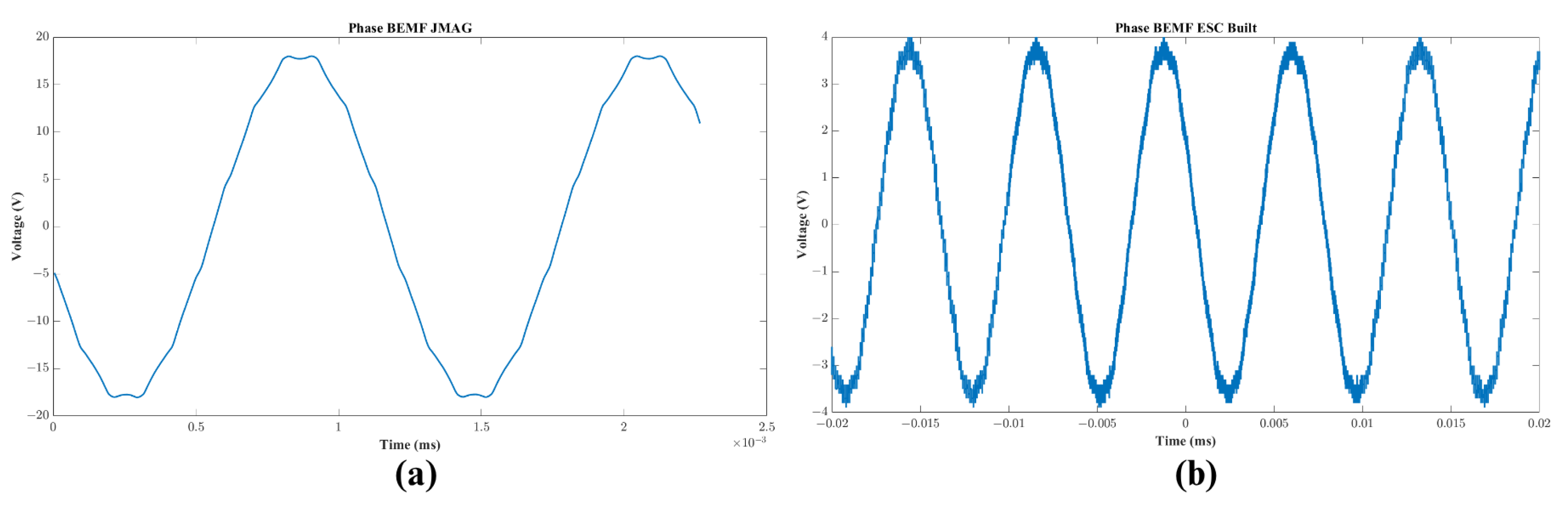
Figure 13.
BEMF: (a) JMAG simulation, (b) measured using a designed ESC with trapezoidal commutation.
Figure 13.
BEMF: (a) JMAG simulation, (b) measured using a designed ESC with trapezoidal commutation.
Figure 14.
Six-step trapezoidal commutation for a three-phase motor with delta termination.
Figure 14.
Six-step trapezoidal commutation for a three-phase motor with delta termination.
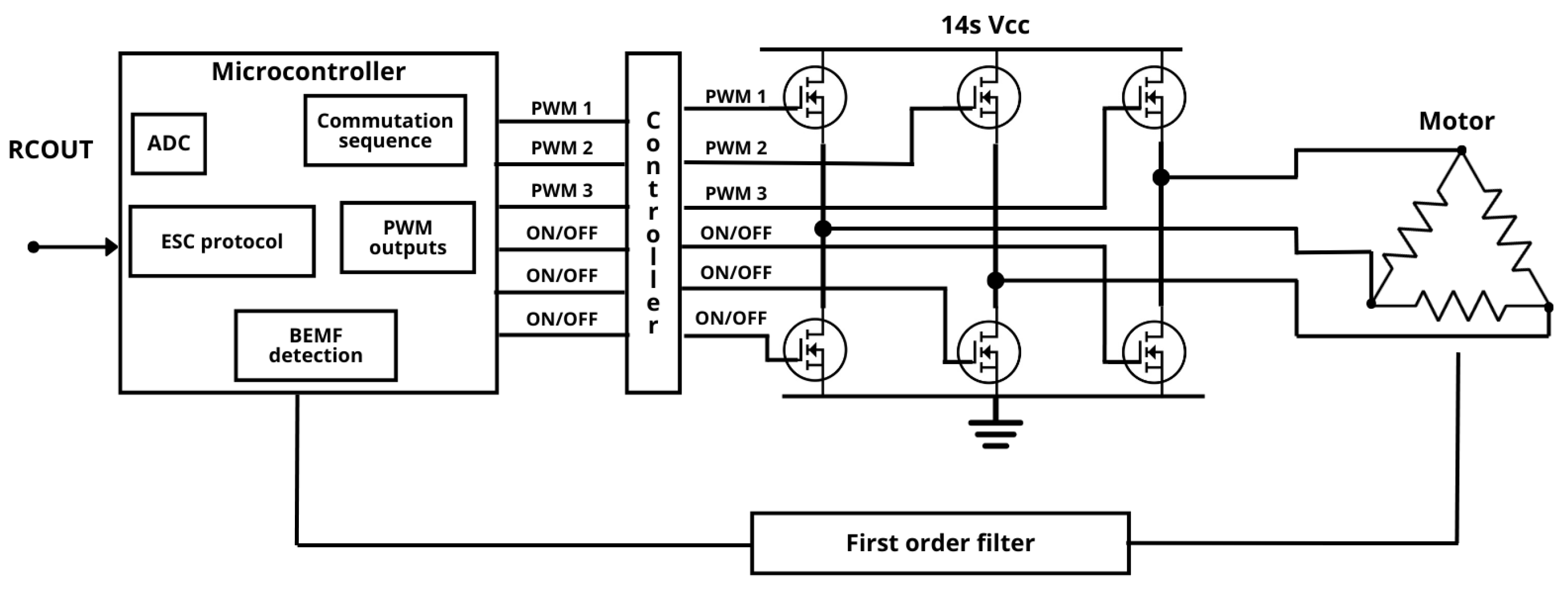
Figure 15.
Electronic speed controller for a three-phase electric motor with delta connection using trapezoidal commutation.
Figure 15.
Electronic speed controller for a three-phase electric motor with delta connection using trapezoidal commutation.
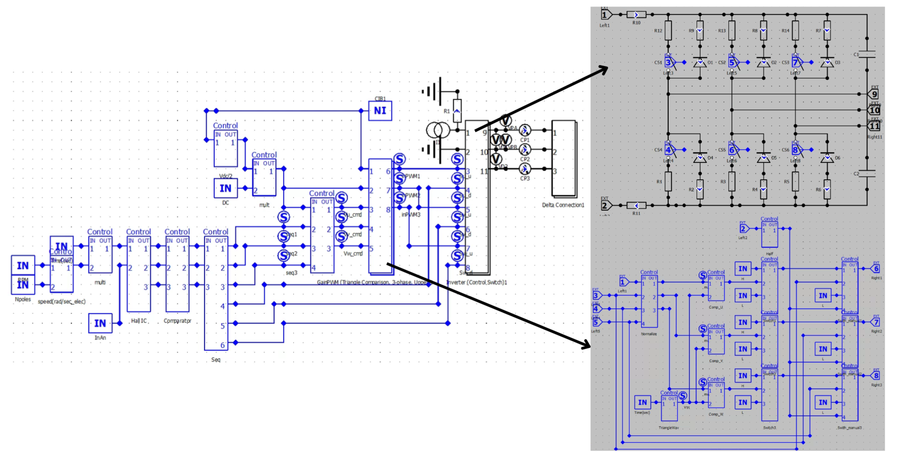
Figure 16.
JMAG circuit for trapezoidal commutation and motor delta connection.
Figure 16.
JMAG circuit for trapezoidal commutation and motor delta connection.
Figure 17.
Magnetic flux density and flux lines for 60% throttle.
Figure 17.
Magnetic flux density and flux lines for 60% throttle.
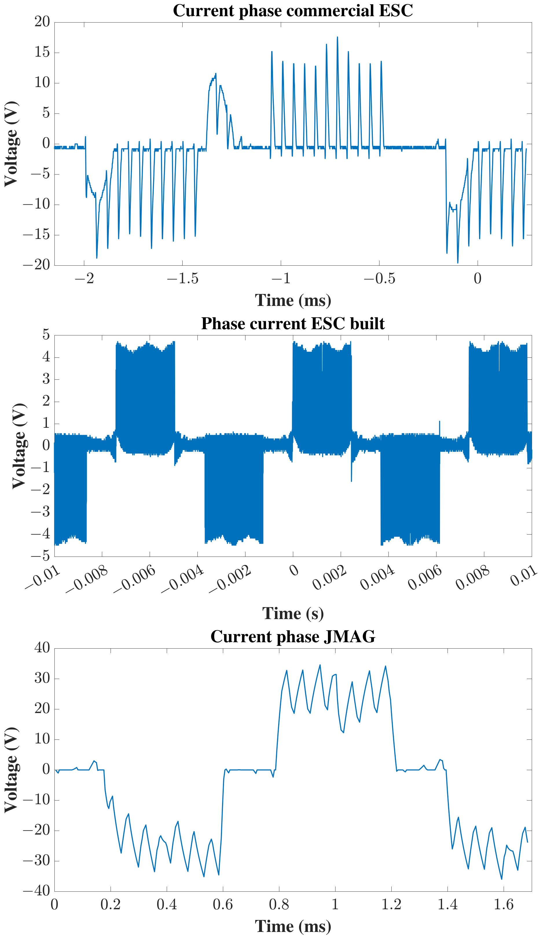
Figure 18.
Phase current qualitative comparison: (top) commercial ESC, (middle) designed ESC, (bottom) JMAG.
Figure 18.
Phase current qualitative comparison: (top) commercial ESC, (middle) designed ESC, (bottom) JMAG.
Figure 19.
Line voltages qualitative comparison: (top) commercial ESC, (middle) designed ESC, (bottom) JMAG.
Figure 19.
Line voltages qualitative comparison: (top) commercial ESC, (middle) designed ESC, (bottom) JMAG.
Figure 20.
Driving signals for 70% throttle from JMAG. (a) Phase currents from JMAG. (b) Line voltages from JMAG.
Figure 20.
Driving signals for 70% throttle from JMAG. (a) Phase currents from JMAG. (b) Line voltages from JMAG.
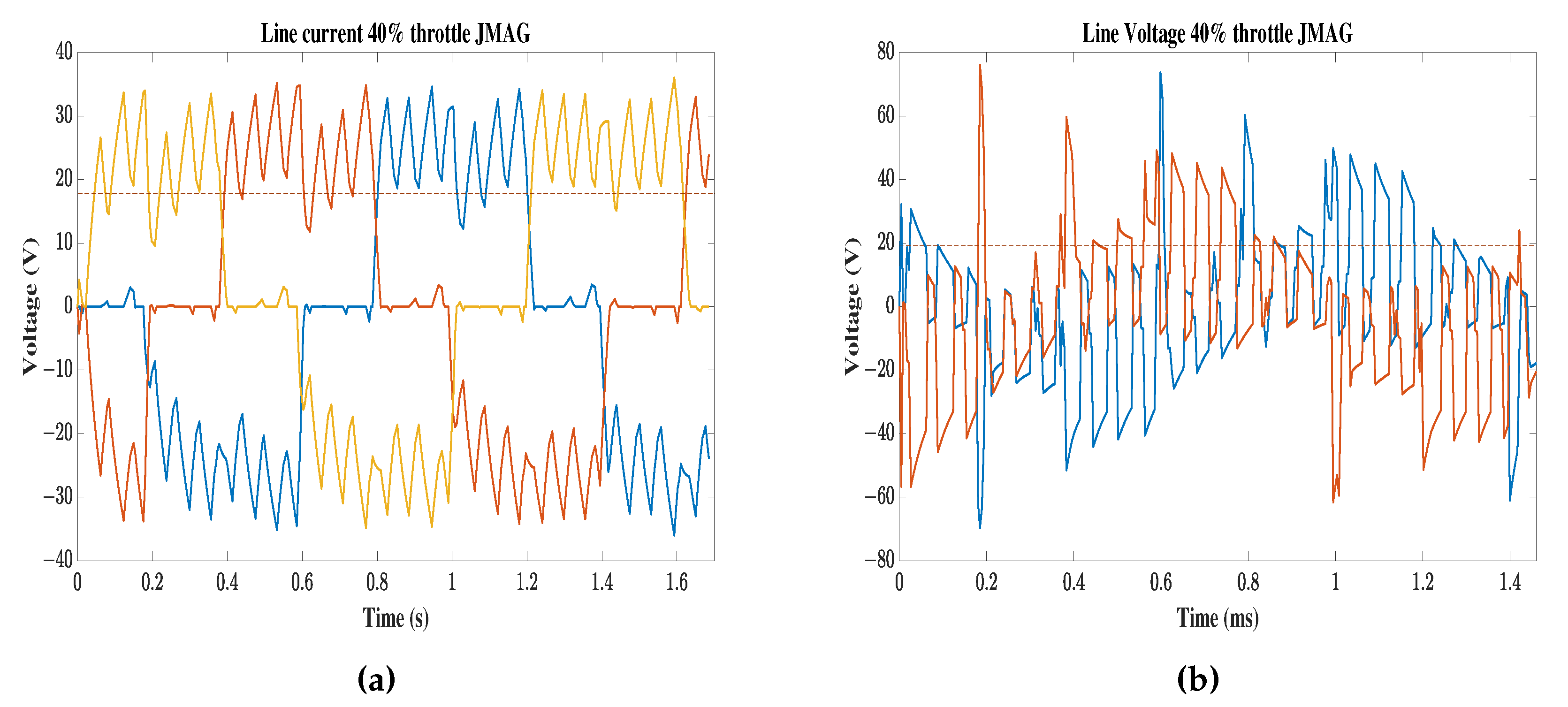
Figure 21.
Driving signals for 40% throttle from JMAG. (a) Phase currents from JMAG. (b) Line voltages from JMAG.
Figure 21.
Driving signals for 40% throttle from JMAG. (a) Phase currents from JMAG. (b) Line voltages from JMAG.
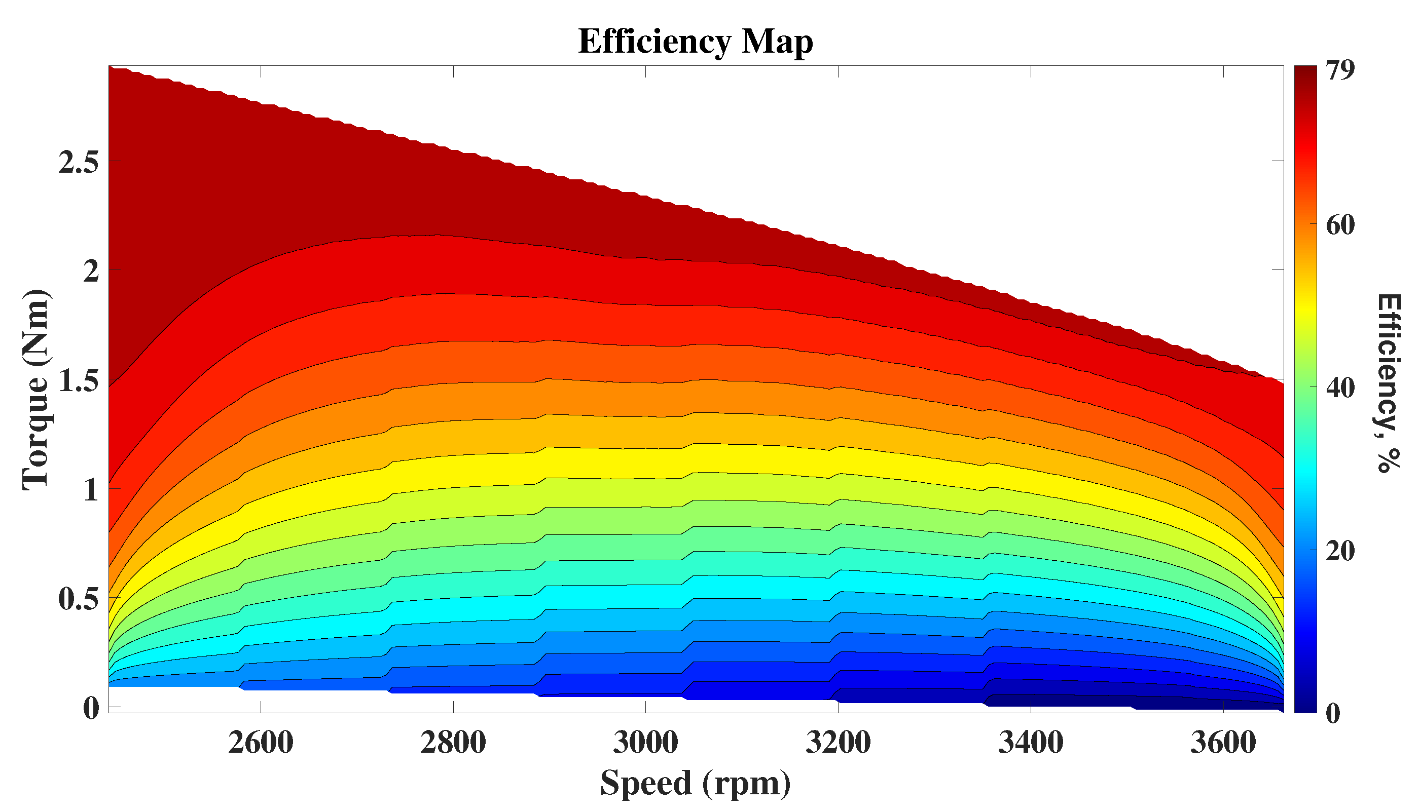
Figure 22.
Reduced motor efficiency map obtained for the expected velocity range.
Figure 22.
Reduced motor efficiency map obtained for the expected velocity range.
Figure 23.
Total losses for the expected velocity range.
Figure 23.
Total losses for the expected velocity range.
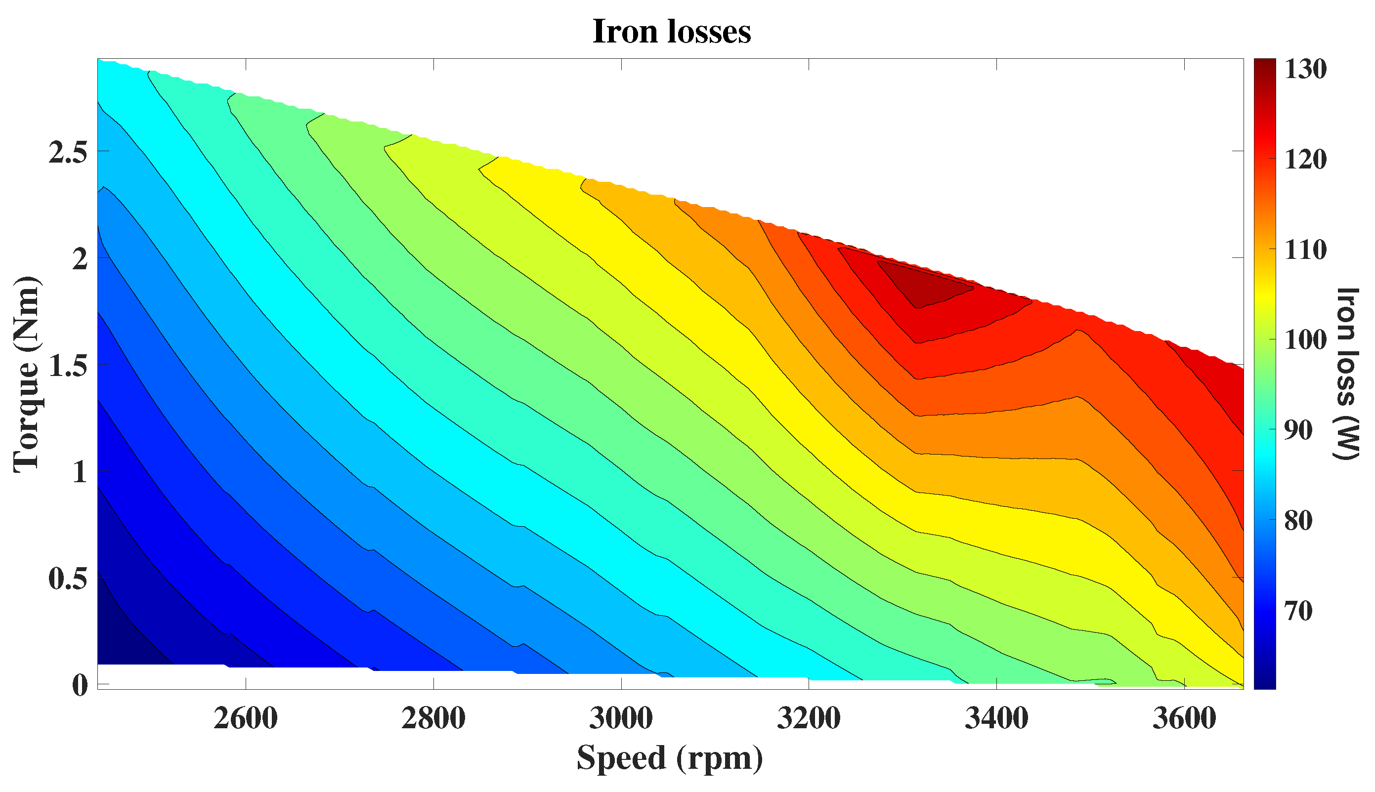
Figure 24.
Iron losses for the expected velocity range.
Figure 24.
Iron losses for the expected velocity range.
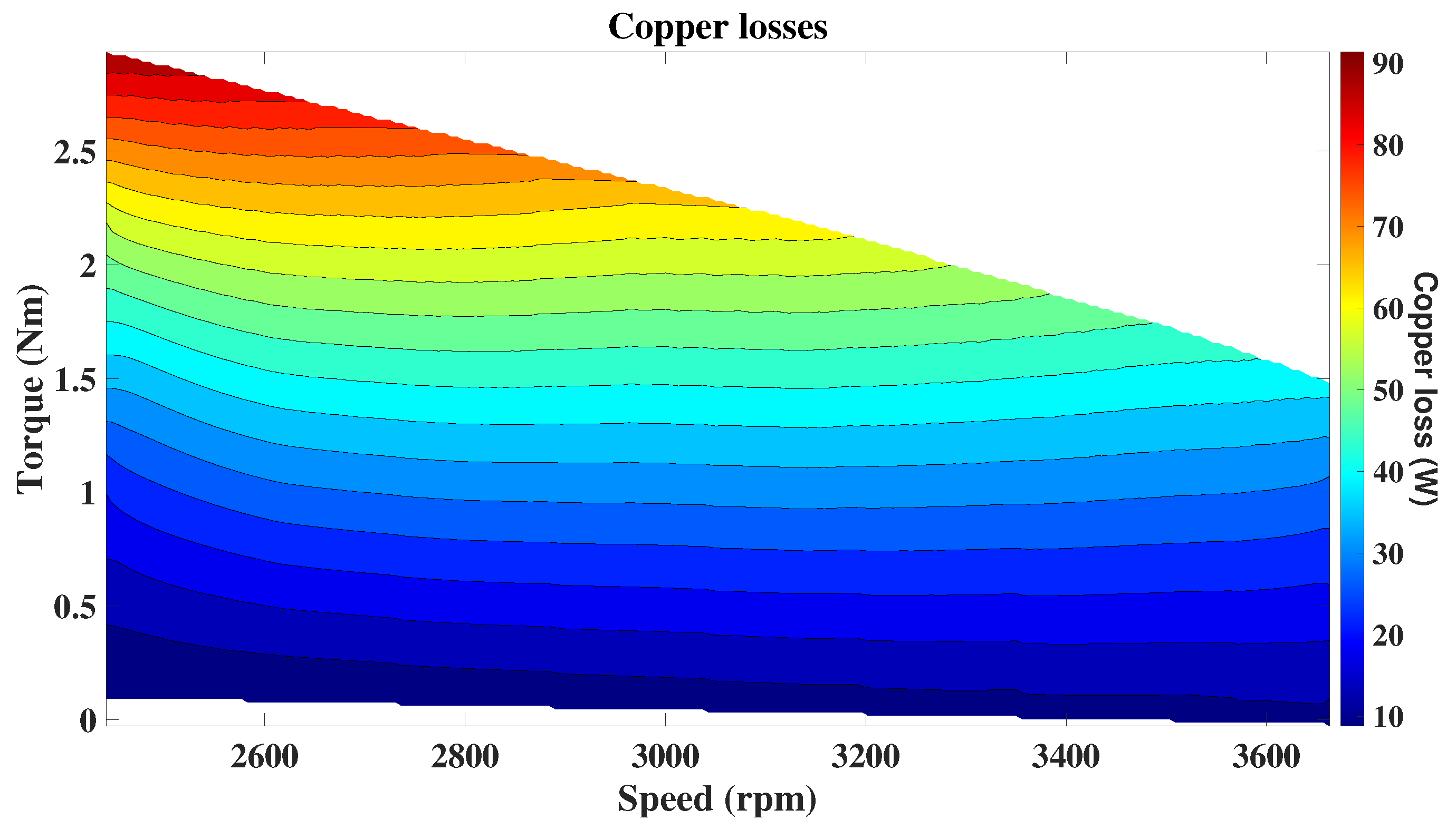
Figure 25.
Copper losses for the expected velocity range.
Figure 25.
Copper losses for the expected velocity range.
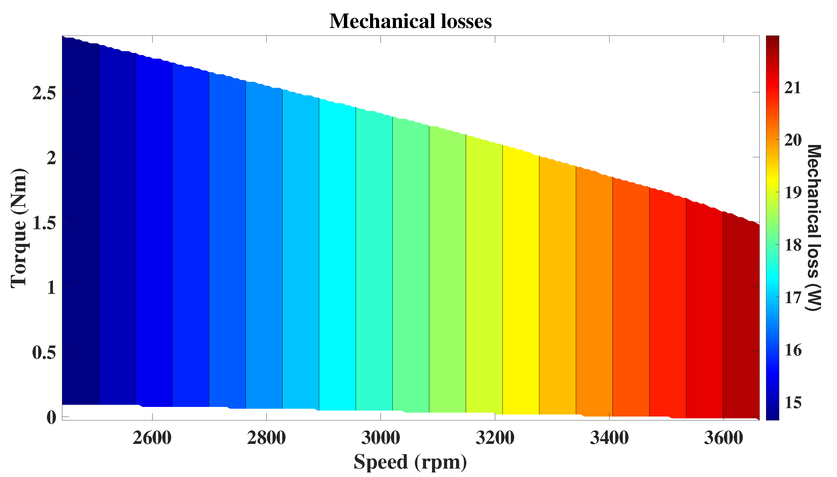
Figure 26.
Mechanical losses for the expected velocity range.
Figure 26.
Mechanical losses for the expected velocity range.
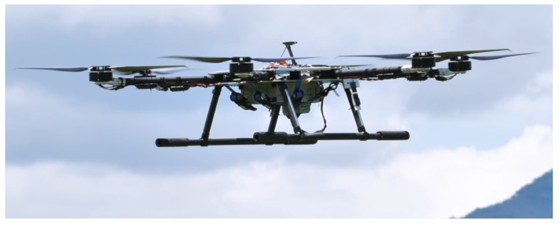
Figure 27.
Propulsion system implementation in a 30 kg large-sized hexarotor.
Figure 27.
Propulsion system implementation in a 30 kg large-sized hexarotor.
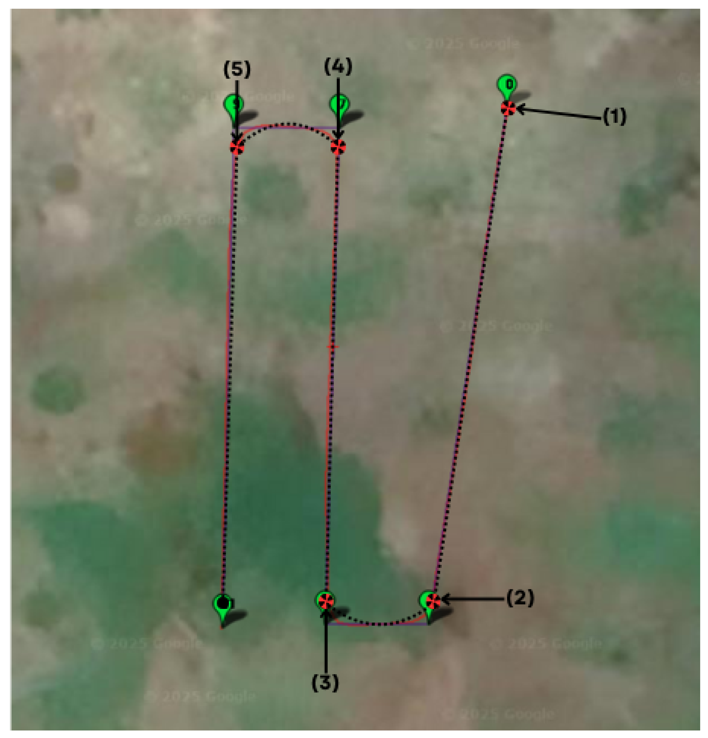
Figure 28.
Trajectory for autonomous flight mode emulating an agriculture application.
Figure 28.
Trajectory for autonomous flight mode emulating an agriculture application.
Figure 29.
Power consumption evolution throughout the imposed trajectory.
Figure 29.
Power consumption evolution throughout the imposed trajectory.
Figure 30.
Evolution of the battery current in the defined trajectory.
Figure 30.
Evolution of the battery current in the defined trajectory.
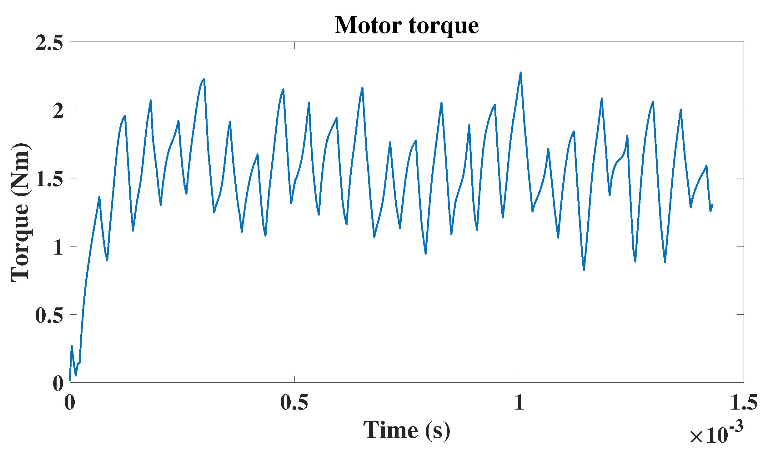
Figure 31.
Motor torque from JMAG corresponding to take-off.
Figure 31.
Motor torque from JMAG corresponding to take-off.
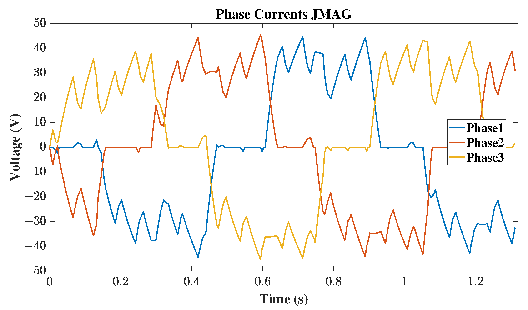
Figure 32.
Three-phase currents from JMAG corresponding to take-off state.
Figure 32.
Three-phase currents from JMAG corresponding to take-off state.
Figure 33.
Motor torque from JMAG corresponding to point four conditions.
Figure 33.
Motor torque from JMAG corresponding to point four conditions.
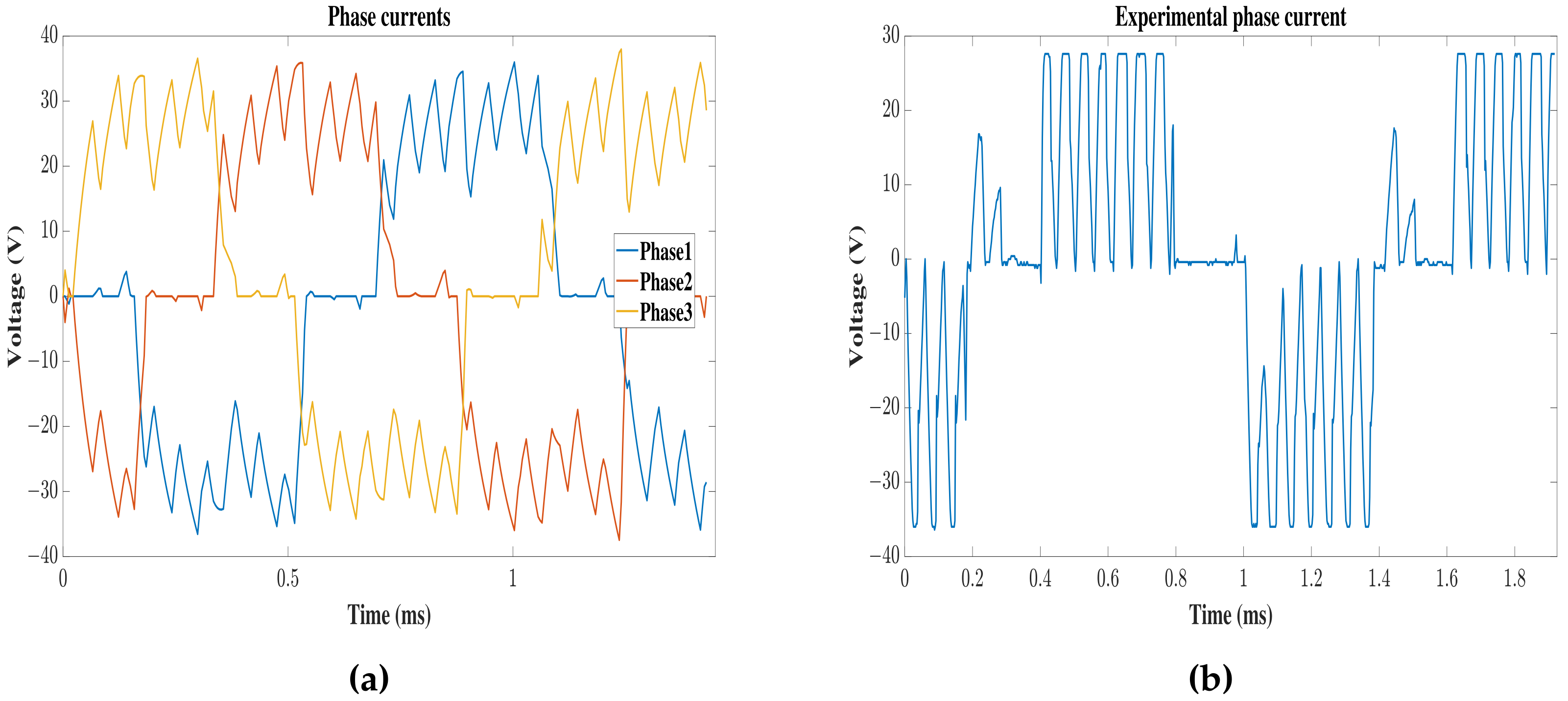
Figure 34.
Motor phase currents for point four in the defined trajectory. (a) Three-phase currents obtained from JMAG. (b) Phase current measured in the static thrust test.
Figure 34.
Motor phase currents for point four in the defined trajectory. (a) Three-phase currents obtained from JMAG. (b) Phase current measured in the static thrust test.
Figure 35.
Motor line voltages for point four in the defined trajectory. (a) Two voltage lines from JMAG. (b) Experimental line voltage measured.
Figure 35.
Motor line voltages for point four in the defined trajectory. (a) Two voltage lines from JMAG. (b) Experimental line voltage measured.
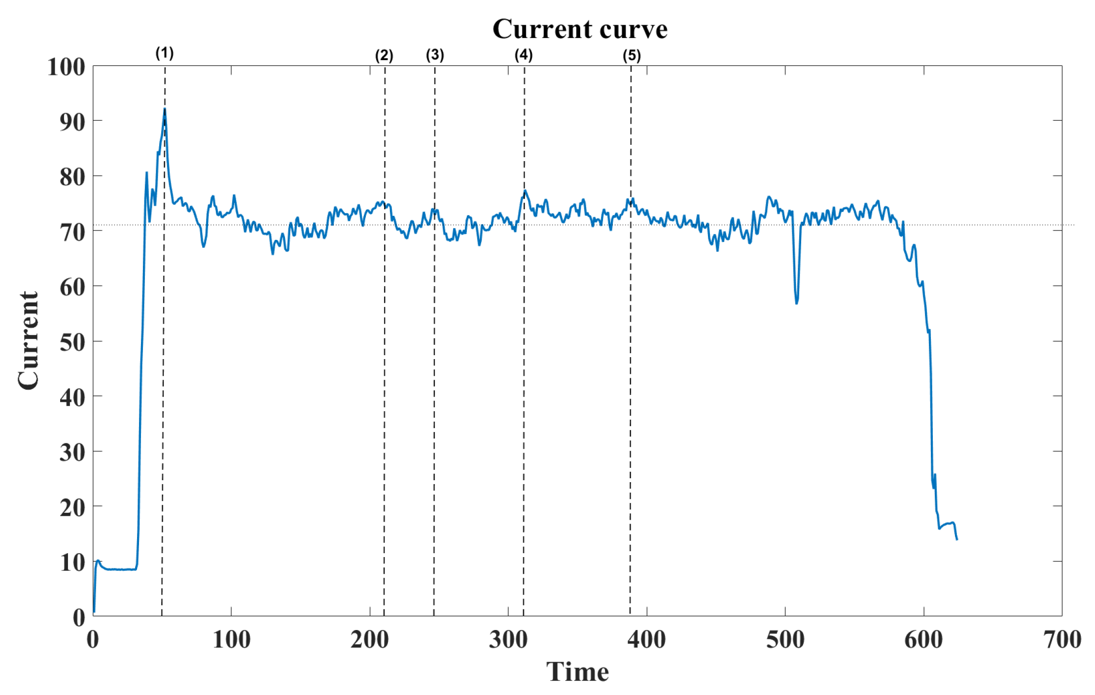
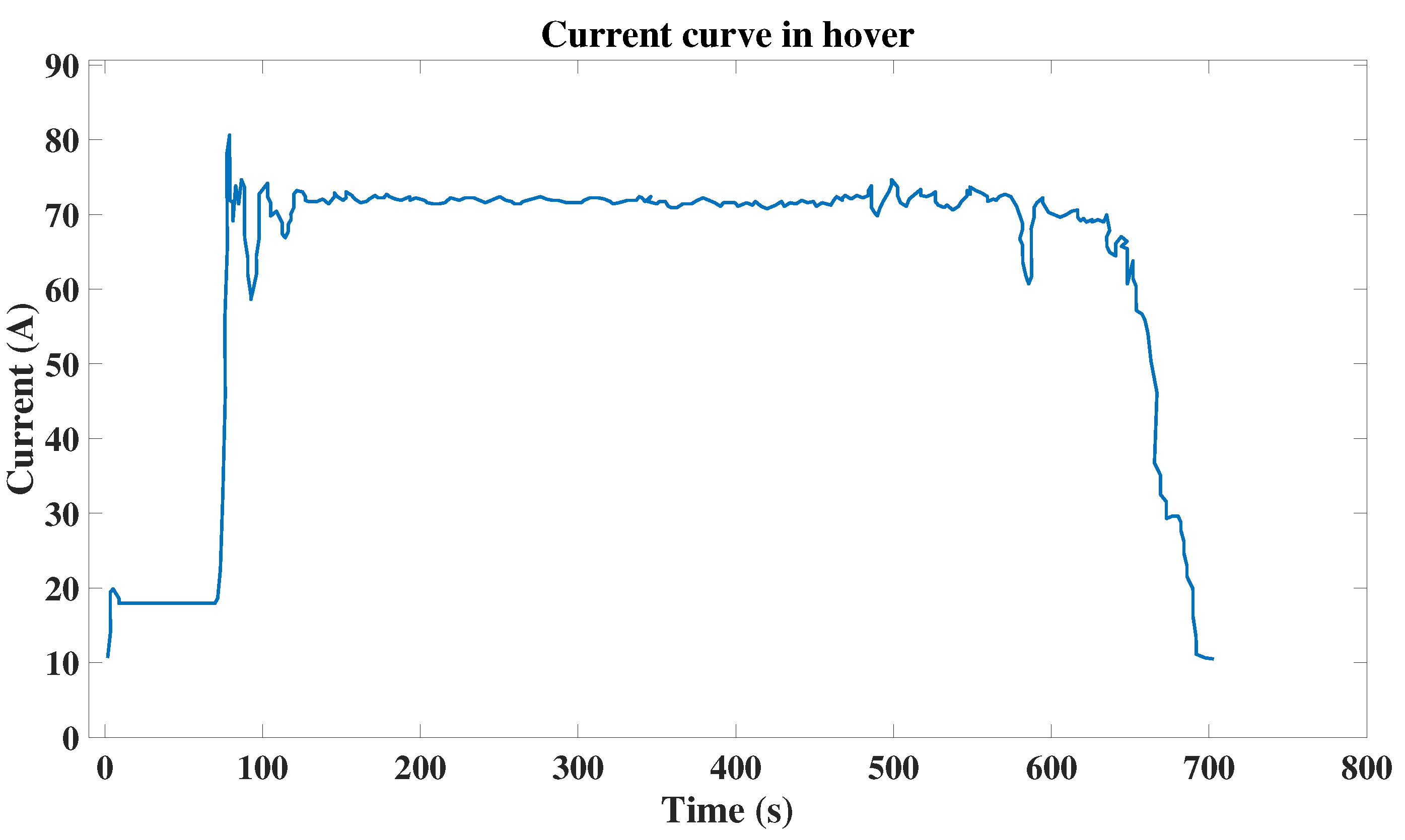
Figure 36.
Current curve for hover test.
Figure 36.
Current curve for hover test.
Table 1.
Basic UAV design requirements for agriculture applications.
Table 1.
Basic UAV design requirements for agriculture applications.
| Design Requirements |
|---|
|
Propeller
|
Motor
|
Battery
|
Structure
|
|---|
| Diameter | KV | Energy density | Take-off weight |
| Pitch | Power | Weight | Maximum dimensions |
| Efficiency | Weight | C-rate | Thrust–weight ratio |
| - | Efficiency | Cells | Weight distribution |
| - | Nominal voltage | - | - |
| Overall efficiency | - | - |
Table 2.
Propeller sizing variables [
2].
Table 2.
Propeller sizing variables [
2].
| Parameter | Value | Unit |
|---|
| 1.225 | kg/m3 |
| 98.1 | N |
| 3200 | rpm |
| 0.1054 | - |
| 2 | - |
| 0.3462 | - |
Table 3.
Boundary conditions for propeller analysis using CFD.
Table 3.
Boundary conditions for propeller analysis using CFD.
| Region | Boundary Condition | Turbulence |
|---|
| Inlet | Pressure inlet | 0.1% turbulence intensity |
| Outlet | Pressure outlet | 0.1% turbulence intensity |
| Static wall | No-slip | - |
| Propeller | No-slip | - |
Table 4.
Thrust and torque validation: numerical and manufacturer data.
Table 4.
Thrust and torque validation: numerical and manufacturer data.
| Error Using Turbulence Model |
|---|
|
RPM
|
Thrust
|
Torque
|
|---|
| 2548 | 4.99% | 10.1% |
| 2971 | 4.69% | 6.7% |
| 3202 | 6.32% | 4.4% |
Table 5.
Motor parameters.
Table 5.
Motor parameters.
| Parameter | Value | Unit |
|---|
| Velocity constant | 120 | rpm/V |
| Motor dimensions | 106.8 × 47.6 | mm |
| Weight | 778 | grams |
| Internal resistance | 22 | mOhm |
| Magnetic configuration | 36N42P | - |
| Nominal voltage | 58.8 | V |
| Iddle current | 1.5 | A |
Table 6.
Motor materials.
Table 6.
Motor materials.
| Parameter | Value |
|---|
| Core | 50CS600H |
| Magnets | Arc N42UH |
| Conductor | Copper |
| Armature | Aluminum |
| Lamination factor | 95% |
Table 7.
Winding characteristics.
Table 7.
Winding characteristics.
| Characteristic | Value |
|---|
| Winding | concentrated |
| Gauge | 23 awg |
| Stator slots | 36 |
| Rotor poles | 42 |
| Phase windings | 12 |
| Pole winding | 0.2857 |
| Pole pitch | 0.85 |
| Conductor threads | 6 |
| Slot conductor turns | 4 |
| Slot fill factor | 33% |
| Termination | Delta |
Table 8.
Typical KV for two different drone applications.
Table 8.
Typical KV for two different drone applications.
| Agriculture Drone | KV | Camera Drone | KV |
|---|
| Agras T10 | 84 | Mavic mini 2 | 2917 |
| Agras T20 | 75 | Mavic 2 pro | 1040 |
| Agras T30 | 77 | Phantom 4 | 800 |
| EFT Z20 | 95 | Inspire 1 pro | 420 |
Table 9.
Circuit parameters for a 60% throttle capacity.
Table 9.
Circuit parameters for a 60% throttle capacity.
| Parameter | Value | Unit |
|---|
| Angular velocity | 3106 | rpm |
| Initial position | 7.18 | degree |
| Modulation ratio | 0.6 | - |
| Nominal voltage | 60.1 | V |
| Inverter bus current | 29 | A |
| Phase inductance | 2.205 × 10⁻⁵ | H |
| Phase resistance | 0.03615 | ohm |
| Inverte branch resistance | 0.5 | ohm |
| PWM’s carrier frequency | 17 | kHz |
| Commutation sequence | u-v-w | - |
Table 10.
Quantitative comparison: JMAG and experimental driving signals for a 70% trottle.
Table 10.
Quantitative comparison: JMAG and experimental driving signals for a 70% trottle.
| Variable | JMAG | Experimental | Error |
|---|
| Phase current | 26.33 A | 26 A | 1.2% |
| Line voltage | 33.12 V | 32 V | 3.5% |
Table 11.
Quantitative comparison: JMAG and experimental driving signals for 40% throttle.
Table 11.
Quantitative comparison: JMAG and experimental driving signals for 40% throttle.
| Variable | JMAG | Experimental | Error |
|---|
| Phase current | 18.707 A | 18.8 A | 0.49% |
| Line voltage | 23.08 V | 22.1 V | 4.43% |
Table 12.
Flight conditions.
Table 12.
Flight conditions.
| Parameter | Value |
|---|
| Take-off weight | 30 kg |
| GPS mode | Auto |
| Maximum altitude | 5 m |
| Flight time | 1.1 min |
Table 13.
Motor–propeller conditions and results for take-off in the specified trajectory.
Table 13.
Motor–propeller conditions and results for take-off in the specified trajectory.
| | Propeller | Motor |
|---|
|
Parameter
|
Simulation
|
Experimental
|
|---|
| Speed | 2735 rpm | 2735 rpm | 2735 rpm |
| Thrust | 60.015 N | - | - |
| Torque | 2.3794 Nm | 2.36 Nm | 2.28 Nm |
| Phase current RMS | - | 24.96 A | 24.2 A |
| Bus current | - | 12.5 A | 12.5 A |
| Mechanical power | 638.67 W | 675.9 W | 653 W |
| Efficiency | 8.97 g/W | 76% | - |
| Overall efficiency | 6.817 g/W | - |
Table 14.
Motor–propeller conditions and results for point four in the specified trajectory.
Table 14.
Motor–propeller conditions and results for point four in the specified trajectory.
| | Propeller | Motor |
|---|
|
Parameter
|
Simulation
|
Experimental
|
|---|
| Speed | 2548 rpm | 2548 rpm | 2548 rpm |
| Thrust | 51.26 N | - | - |
| Torque | 2.092 Nm | 1.95 Nm | 1.93 Nm |
| Phase current RMS | - | 22.6 A | 21.4 A |
| Bus current | - | 11.2 A | 11.2 A |
| Mechanical power | 542.71 W | 520.29 W | 514.9 W |
| Efficiency | 9.31 g/W | 76% | - |
| Overall efficiency | 7.075 g/W | - |
Table 15.
Comparative analysis of large-sized multi-rotors.
Table 15.
Comparative analysis of large-sized multi-rotors.
| Parameter | Proposed Drone | Agras T10 | Agras T20 | Coaxial Drone [26] |
|---|
| Take-off weight | 30 kg | 24.8 kg | 32 kg | 20 kg |
| Motor KV | 120 rpm/V | 84 rpm/V | 48 rpm/V | 330 rpm/V |
| Max motor power | 4560 W | 2500 W | 4000 W | 1425 W |
| Flight time in hover | 11.6 min | 9 min | 14.5 min | 9.88 min |


 ,
, 


