An Agent-Based Simulation and Optimization Approach for Sustainable Urban Logistics: A Case Study in Lisbon

Abstract

Urban logistics plays a crucial role in ensuring the efficient movement of goods in densely populated areas. This study examines the PDP-TW in an urban logistics context using an integrated approach that combines an agent-based simulation model and an optimization model. The research focuses on a real-world case study, comparing the company’s current operational scenario with an optimized scenario generated through a PDP-TW model adapted from the literature. The findings reveal that the optimized model reduced the total distance traveled by approximately 38%, while the simulated optimized scenario achieved a reduction of about 36.5%. Consequently, the total cost decreased from EUR 116.50 in the real-world operations to EUR 71.21 in the optimization model and EUR 73.29 in the simulated optimal real scenario. Additionally, the optimized approach required only two drivers instead of three, indicating potential efficiency gains in resource allocation. In the optimization model, window constraints were strictly satisfied. However, in the agent-based simulation, a few deliveries were completed within the 10 min empirical tolerance threshold, rather than within the scheduled window itself. This outcome underscores the need for enhanced scheduling strategies to increase time window robustness under real-world execution variability. Despite these advancements, the ABS model remains deterministic and does not account for uncertainties such as traffic congestion or vehicle breakdowns. Future work should incorporate stochastic elements and evaluate the model’s scalability with a larger dataset and instances to better understand its applicability in real-world logistics operations.

1. Introduction

Urban logistics has emerged as an interdisciplinary field encompassing various areas of knowledge, highlighting its significance in the face of global urban transformations. Population growth and urban concentration have driven an increasing demand for more efficient and sustainable transportation and distribution systems [1]. Furthermore, shifts in consumer behavior, such as the rise in online shopping and growing environmental concerns, intensify logistical challenges while fostering innovative solutions to minimize impacts and maximize the efficiency of urban operations. According to Moreno et al. [2], the field of urban logistics remains fragmented, making it challenging to achieve a holistic understanding and identify critical research gaps. Despite this, systematic studies, such as those by Lagorio et al. [3] and Frederhausen and Klumpp [4], have advanced the field by addressing core challenges, including Location-Routing Problem (LRP), Transshipment Location Problem (TLP), and Pickup and Delivery Problem (PDP).

PDP stands out among these problems due to its complexity and its pivotal role in enhancing operational efficiency and sustainability in urban logistics. Moreno et al. [2] mention that PDP focuses on optimizing the movement of goods between specific origins and destinations, considering constraints such as time windows, capacity, and urban traffic dynamics. Its prominence in the literature underscores its importance in addressing the growing demands of modern urban environments, making it a key area for technological and methodological advancements in the field. In the classical PDP formulation, a set of capable vehicles must be selected to fulfill customer requests. The request consists of picking up the merchandise at the original point and delivering it to the destination point. The same vehicle can carry multiple requests at the same time, if the total load does not exceed its capacity. For each request, the visit to the point of origin must occur before the visit to the point of destination. Furthermore, both locations must be visited by the same vehicle, except in cases of transshipment, where the order may be fulfilled by another available car. Each destination of origin and destination must be visited exactly once.

Given the significance of the problem and the rise in e-commerce driven by advancements in communication technologies, the PDP and its variants have garnered increasing attention in recent years [5,6]. One of the variants introduces transshipment points, leading to the formulation of the Pickup and Delivery Problem with Transshipment (PDP-T) in the literature [6,7]. Unlike the classic PDP, the PDP-T permits goods to be transported by multiple vehicles. According to Lyu and Yu [6], this approach optimizes time and vehicle capacity utilization, offering potential enhancements in logistics operations. Furthermore, time constraints are a critical factor in real-world scenarios, influencing order receipt and delivery. This consideration introduces an additional variable, resulting in the Pickup and Delivery Problem with Time Windows and Transshipment (PDPTW-T)

Although PDP has been addressed for some time [8], most problems related to it do not consider uncertainty. Typically, the approaches used are deterministic, meaning that it is assumed that the problem data are known beforehand, which can lead to solutions that are considered admissible, but may not be valid in practice due to data variations. [2].The integration of agent-based simulation (ABS) and discrete-event simulation (DES) techniques represents a robust and innovative approach to overcoming the limitations of traditional models in urban logistics. As highlighted by Moreno et al. [2], simulation techniques provide a dynamic, adaptable, and detailed framework capable of modeling complex and heterogeneous interactions among the various agents and processes that comprise urban logistics networks. This approach is particularly effective for addressing scenarios involving environmental uncertainties and variabilities, such as traffic fluctuations, delays in pickups and deliveries, and unforeseen changes.

Furthermore, studies such as those by Martinez [9] and Murarețu and Bădică [10] have applied their research to PDP, demonstrating the applicability and effectiveness of ABS integration in capturing emerging behaviors, enabling in-depth analyses of logistics operations and evaluating performance optimization strategies under realistic conditions. These methods are fundamental in solving problems such as the PDP and its variants by combining flexibility in modeling operational dynamics with the capability to test scenarios and make data-driven decisions. This integrated approach stands out as an important tool for improving the efficiency, sustainability, and resilience of operations. For further insights into the application of simulation in logistics, we recommend the work of Mehdizadeh et al. [11].

This study applies an ABS model to analyze the PDP-TW in a real-world case study in Lisbon. The company specializes in luggage collection and delivery, ensuring adherence to client-specified time constraints and, when necessary, utilizing temporary storage facilities. For comparison, a pre-existing optimization model, based on PDP-TW and adapted to the specific requirements of this case, was incorporated to represent the steady-state behavior of operations. The ABS model captures the dynamic interactions between key logistical entities, such as transport vehicles, pickup points, delivery locations, and storage facilities, offering a comprehensive representation of the company’s logistics network. By integrating simulation and optimization, the study aims to compare the company’s current operations with an optimized scenario, evaluating route efficiency, cost minimization, and time window adherence. Furthermore, the research explores the impact of route optimization on sustainability, highlighting the reduction in total traveled distance and its direct correlation to CO₂ emissions, given that the company operates a non-electric vehicle fleet. The findings demonstrate that optimization and simulation together can significantly enhance operational efficiency, providing actionable insights for improving resource allocation and urban logistics performance.

This paper is structured as follows. In Section 2, a focused literature review covering existing research on methodologies used in urban logistics, including ABS for the context of PDPs, is presented. In Section 3, the material and methods are detailed, describing the problem context, the PDP-TW mathematical model, and the ABS model. Section 4 describes the case study in the city of Lisbon, including the validation of the proposed simulation model (ABS). Section 5 presents the results and discussion of the simulation with data provided by the company under study. Finally, conclusions, implications and possible future research directions are presented in Section 6.

2. Literature Review

Urban logistics is an area of extreme importance for the functioning of a city, since it is directly related to the transportation of goods, services and people. However, urban logistics presents several challenges, such as the complexity of transportation systems, the variation in demands, and the presence of multiple agents involved [10]. In urban logistics, the supply chain must be highly efficient and adaptable to meet growing demands, especially those driven by the advancement of e-commerce and the need for fast deliveries in densely populated areas. As highlighted by Rao et al. [12], the strategic location of logistics centers plays a fundamental role in the performance of the supply chain, contributing to the reduction in operational costs and the improvement of efficiency in the distribution of goods. In addition, the integration of these centers with optimized transportation routes ensures the agile and economical delivery of products, a critical aspect in urban environments marked by intense competition for space and time resources. The strategic location of logistics centers and their integration with optimized routes, which are fundamental for the efficiency of urban logistics, have direct implications for the solution of Vehicle Routing Problems (VRPs), especially in the subcategory known as PDP.

PDP involves the transportation of objects or people between specific origins and destinations and can be classified into three main categories. The first group, many-to-many, allows any node to function as an origin or destination for any commodity. A classic example is the exchange problem, as described by Anily and Hassin [13], where each node initially contains one type of commodity and requires another specific type. The second group, one-to-many-to-one, addresses scenarios in which goods are sent from a warehouse to several customers, with pickups returning to the warehouse, as in the study by Mitrović-Minić and Laporte [5], which proposes optimized solutions to maximize operational efficiency. Finally, the one-to-one group encompasses situations in which goods have specific origins and destinations, common in express mail operations and door-to-door services. Santos et al. [14] explored this category by analyzing differences between taxi and ridesharing, highlighting that both approaches involve transportation requests with a defined origin and destination.

The growth of e-commerce, combined with advances in information technology, which allows online service requests as observed in the company under study, has generated the need for new approaches to optimize transportation systems. One such approach is the inclusion of transshipments in the logistics process, resulting in the PDP-T. Recent studies, such as Tadei et al. [15], explore the PDP-T by analyzing how uncertainties in goods handling can be managed to improve logistics performance, highlighting its potential in complex and high-demand urban scenarios. For a detailed overview of the main works on PDPs applied to urban logistics, see Moreno et al. [2], which is a systematic review of three important approaches in logistics: PDP, TLP and LRP. However, recent methodological developments in PDP-TW literature demonstrate a shift towards more adaptive, realistic, and robust models that incorporate uncertainty and operational constraints. For example, Abreu [16] propose a robust optimization framework that integrates travel time uncertainty directly into the mathematical formulation of PDP-TW, generating solutions that maintain feasibility across a predefined set of adverse scenariosc improving resilience in fluctuating traffic conditions. Similarly, Khanna et al. [17] introduce the PDPTW-DB (Driver Breaks) model, a Mixed-Integer Linear Programming (MILP) based formulation that incorporates driver break regulations, illustrating the importance of regulatory compliance and human constraints within route planning, elements commonly overlooked in traditional PDP-TW formulations.

Genetic algorithms (GA) remain a prevalent method for solving PDP-TW variants, particularly under multi-objective and constrained environments. Dridi et al. [18] proposed a GA framework targeting the simultaneous minimization of vehicle count, total waiting time, and travel distance. Their approach uses adjacency-based chromosome representations and tailored genetic operators to maintain solution feasibility, with optimization driven by Pareto dominance without the need to aggregate objectives. In a more recent advancement, Ma et al. [19] developed an adaptive genetic algorithm integrated with neighborhood search heuristics for optimizing O2O (online-to-offline) takeaway deliveries via electric bikes with varied compartment configurations. Their method introduces adaptive crossover and mutation strategies guided by local search to enhance convergence in dynamic urban delivery settings. While both studies rely on GAs to solve complex routing under capacity and time constraints, Harbaoui Dridi et al. focus on structural multi-objective balance in classical PDP-TW formulations, whereas Ma et al. embed modern delivery logistics constraints, such as vehicle heterogeneity and customer time preferences, into a hybrid evolutionary scheme. Together, these contributions showcase the methodological evolution of GAs from foundational multi-criteria optimization toward more nuanced and operationally grounded PDP-TW applications.

Given its relevance and the associated challenges, urban logistics stands out as a rich and significant field of study. In the context of the PDP, ABS has proven to be effective in modeling complex and dynamic logistics systems. ABS is particularly well-suited for systems involving multiple autonomous participants that interact and adapt dynamically to changes within the environment [20]. In ABS, models are built using entities called agents, which interact within an environment. These agents are autonomous, capable of communication, decision-making, and pursuing objectives based on defined behaviors and rules. Each agent operates as an intelligent entity with specific conditions and interests, making decisions dynamically based on its environment and interactions. The flexibility of ABS makes it an ideal choice for modeling complex, non-linear, and dynamic behaviors. It allows for the incorporation of geographic features using maps, linking cost and time metrics at the agent level, and providing detailed visualizations. These visualizations are valuable not only during model development but also for effective communication with end-users and decision-makers. Martinez et al. [9] explored an ABS model applied to shared taxi transportation in Lisbon, demonstrating how this approach can manage dynamic interactions among agents and improve operational efficiency. The study emphasized that agent-based models are ideal for capturing emergent behaviors and spatial-temporal complexities, enabling urban scenarios to be modeled with greater accuracy. This capability is particularly valuable in densely populated urban environments, where demand fluctuations and infrastructure constraints can directly impact operational performance.

Additionally, Muraretu and Bădică [10] presented an ABS approach for the PDP with time window constraints and electric vehicles (PDPTW-EV). Their study introduced consensus mechanisms as an order allocation strategy, showing that this approach not only optimizes fleet utilization and minimizes costs but also promotes sustainable solutions by integrating electric vehicles into urban logistics. The results indicated that agent-based simulation, combined with consensus strategies, effectively handles uncertainties and operational constraints, highlighting its applicability in modeling and optimizing dynamic and sustainable urban transport scenarios.

Taken together, the studies reviewed highlight the increasing relevance of ABS as a robust methodology for modeling and optimizing complex urban logistics systems, particularly within the scope of the PDP and its variants. From the modeling of dynamic passenger flows by Martinez et al. [9] to the integration of sustainability through electric vehicle fleets in the PDPTW-EV model proposed by Muraretu and Bădică [10], ABS approaches have demonstrated strong capabilities in handling both operational complexity and environmental constraints. These contributions suggest that ABS is not only effective in replicating real-world logistics behaviors but also serves as a powerful decision-support tool in environments characterized by high variability and operational limitations. Nevertheless, despite notable advancements in PDP modeling, there remains a gap in the literature regarding the integration of ABS with mathematical optimization models, particularly when applied to real-world companies operating under time window constraints, as seen in the PDP-TW.

This study addresses this gap by proposing a hybrid framework that integrates an adapted PDP-TW optimization model with an ABS approach, applied to real operational data from an urban luggage transportation company. By comparing the company’s actual performance with that of an optimized scenario, the research not only validates the ABS model against real-world outcomes but also demonstrates its potential to identify logistical inefficiencies, reduce operational costs, and minimize CO₂ emissions—contributing to more sustainable urban logistics practices. This dual-method approach (simulation and optimization) enhances the methodological foundation for PDP-TW applications and provides a foundation for future research focused on incorporating uncertainty and scalability into urban logistics modeling.

3. Materials and Methods

This study proposes an ABS approach to address logistics operations and applies it to real-world data from a case company. The company focuses on the pickup and delivery of goods, primarily luggage of various sizes (i.e., small, medium, and large), in several European cities, such as Athens, Barcelona, Budapest, Lisbon, and Porto, among others. In its operational context, each service request includes a predefined collection and delivery location and must be executed within a specified time window, with a minimum of two hours’ scheduling notice. Routes are dynamically generated according to demand, and loads are consolidated whenever vehicle capacity allows. In cases where the vehicle cannot complete the delivery on the same day or when it exceeds its capacity, temporary storage in a fixed warehouse is employed. While each region presents unique operational challenges, the company must meet customer-specific requirements under strict time constraints and limited resource availability.

To address this issue, two methodologies are applied: (1) an adapted PDP-TW model from literature to represent the steady-state behavior of the logistics system and serving as a validation tool for the simulation model, where this model employs the Geodisc function to compute distances between points, using the standard WGS-84 ellipsoid implemented by Geopy package [21], and (2) an ABS implemented using the AnyLogic PLE platform [22]. This simulation is enhanced with geographically specific data adapted to the study area, Lisbon, Portugal, utilizing a Geographic Information System (GIS) for improved visualization. Applying these two methods is essential to assess the accuracy and applicability of each approach, enabling a more robust modeling of the logistics network. By integrating these methodologies, the study provides a comprehensive and dynamic framework for modeling, analyzing, and optimizing the company’s logistics network, effectively addressing real-world variability and operational constraints.

An adapted version of the optimization model proposed by Lyu and Yu [6] is used in this study to reflect the specific operational constraints of the case company. The PDP-TW optimization model generates optimal operational scenarios based on real-world input data from the company, in which this adapted model also acts as a reference to validate the ABS model, in addition to providing inputs for the ABS model to simulate and evaluate the dynamic behavior and feasibility of these optimized solutions within the urban logistics environment.

The simulation is organized into a logical sequence based on input processes, behavior, and output data. This approach reflects the dynamics of the modeled operations, ensuring an accurate representation of interactions and expected outcomes. The input data for the simulation includes the characteristics of the entities/agents involved. Each request, representing a client’s pickup and delivery order, contains attributes such as luggage size (i.e., small, medium, or large), pickup and delivery locations defined by geographic coordinates (i.e., latitude and longitude), and the associated operation times. Vehicles, responsible for transportation, are described by attributes including a maximum capacity of 24 volumes, initial location in warehouse, and estimated travel time calculated based on distances between points. Additionally, the model considers optional fixed warehouses with defined locations, maximum storage capacities, and associated operational costs.

The behavior of the agents is governed by rules and processes that reflect real-world operations. Orders are sorted and allocated based on baggage size and vehicle availability. When demand exceeds vehicle capacity or there are discrepancies between collection and delivery dates, orders can be directed to fixed warehouses. Alternatively, vehicles can function as mobile warehouses, respecting volume and time restrictions. Deliveries are prioritized to be completed within the timeframe established by the customer. In addition, the model incorporates the company’s tolerance policy, which establishes that scheduled baggage collection and delivery times can occur up to 10 min late.

The simulation generates detailed data on system performance, including the number of requests served, vehicle and depot utilization rates, and average travel times. Metrics such as operating costs, warehouse efficiency and adherence to deadlines are recorded to assess the effectiveness of the strategies implemented. This modular structure allows bottlenecks to be identified and adjustments to optimize baggage transportation and storage, increasing efficiency and meeting operational demands. A critical analysis is made between the optimization model and the ABS model, using real-world operational data from the company under study, which promptly provided quantity of 24 orders from the months of December/2022 and January/2023 for the adaptation of the optimization model and generation of the simulation model.

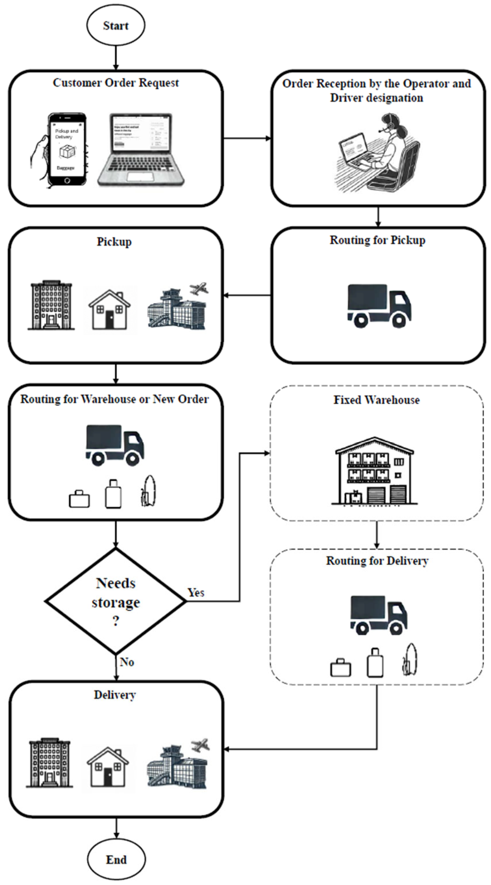
3.1. Conceptual Model

The simulation model serves as a structured platform to explore feasible solutions to the problem and conduct the proposed experiments. To achieve this, a simulation model was implemented, integrating the main activities associated with the approach widely recognized in the literature as the PDP, using SBA. This subsection presents the conceptual model that underpins its implementation. Figure 1 illustrates the concept of the modular simulation model, highlighting its interfaces and interconnected components.

The conceptual model organizes and represents the key agents, behaviors, and interactions underlying the simulation. It provides a structured foundation for implementation, ensuring consistency with the PDP and addressing the specific operational requirements of the logistics network of the company under study.

Agents and Attributes

The model identifies three primary agents:

• Order: Represents customer requests for pickup and delivery|Attributes include size (small: 1 unit, medium: 2 units, large: 4 units), geographic coordinates for pickup and delivery, and specific time windows.
• Vehicles/Drivers: Responsible for transporting luggage between locations|Attributes include maximum capacity (24 units), dynamic positioning during operations, and estimated travel time based on geographic distances.
• Warehouses: Fixed locations for temporary storage of luggage, used when operational constraints prevent direct delivery|Attributes include storage capacity and associated operational costs.

Rules and Behaviors

The simulation operates based on predefined rules:

• Order Classification and Allocation: Orders are assigned to vehicles based on their size and the vehicle’s available capacity, ensuring the total does not exceed 24 units.
• Storage Decisions:

  ○

  If the pickup date and the delivery date do not match, the goods are sent to a warehouse.

  ○

  Condition 2: If the vehicle has sufficient capacity, it acts as a mobile warehouse.

  ○

  Condition 3: If the vehicle does not have sufficient capacity, the goods are sent to a warehouse with the help of a vehicle designated for this situation.

• Time Window Compliance: Pickup and delivery times are subject to a 10 min tolerance to account for operational delays.
• Safety Assurance: Once the baggage is collected, the company under study assumes full responsibility for its safe transportation and storage.

Key Interactions

• The simulation captures interactions between agents, such as:
• Vehicles consolidating or exchanging cargo at meeting points to optimize routes and capacity usage.
• Dynamic reassignment of orders based on real-time changes in vehicle availability and capacity.

Performance Indicators

The conceptual model defines key metrics to evaluate and compare both the ABS and the optimization approach:

• Capacity utilization: percentage of vehicle capacity utilized.
• Time: task time and length of time luggage remains in storage facilities.
• Distance travel: the distance per task and total for all vehicles.
• Number of Vehicles Used: Total vehicles required to fulfill all orders.
• Time Window Adherence: Percentage of pickups and deliveries completed within the allowed time tolerance.
• CO₂ Emissions: Estimated carbon dioxide emissions based on the distance traveled and fuel consumption of diesel vehicles, used to assess the environmental impact of each scenario.

Regarding integration and implementation, the conceptual model aligns with the ABS framework implemented using AnyLogic PLE (version 8.9.0). This approach leverages GIS data for accurate geographic representation and visualization, facilitating the incorporation of real-world variability into the simulation. Additionally, the optimization model serves as a benchmark for validating the ABS, ensuring the simulated dynamics adhere to established logistical standards.

The validation of the conceptual model developed in this simulation is primarily based on critical analysis and consensus reached with specialists from the company under study. The behaviors represented in the conceptual model were derived from observations of similar systems and in-depth discussions conducted during meetings with the company’s team. Each key behavior was designed and evaluated based on direct observation of the company’s processes, ensuring greater alignment with operational reality. The conceptual model diagram provides a detailed and justified representation of the behaviors incorporated into the simulation, serving as the foundational framework for building a functional and executable simulation model.

To ensure the accuracy and reliability of the simulation model, validation focuses on four critical aspects: the correct execution of the process flow according to the defined rules, the effective interactions between agents (Order, Vehicles, Warehouse), and the comprehensive assessment of costs, times, and capacities across various simulated scenarios. Additionally, the validation includes a comparison with a PDP optimization model selected from the literature. This optimization model will be applied to the same problem addressed by the simulation, enabling a detailed analysis and comparison of results between the two approaches to validate the simulation model.

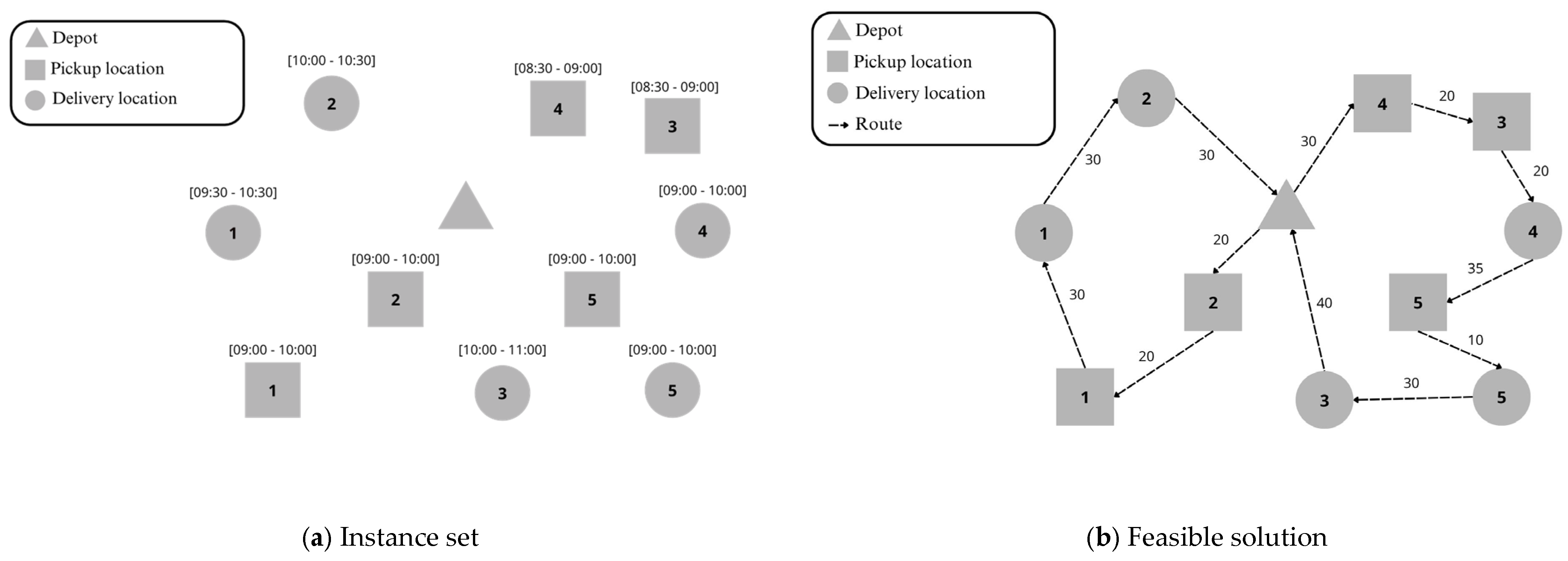
3.2. Mathematical Model Formulation

The PDP-TW was formulated as a MILP model based on the adaptation of the model proposed by Lyu and Yu [6], while excluding the transshipment component. This modification is justified by the fact that the company under study does not utilize transshipment points in its logistics operations, making it inappropriate to retain this characteristic in the model. Therefore, its removal was essential to ensure the model aligns with the operational reality being analyzed.

The notations are defined as follows. Let $R$ be the set of requests. Let $G=\left(V, A\right)$ be a directed graph, where $V$ and $A$ are the set of vertices and arcs, respectively. The set of vertices $V$ is defined as $V=O\cup O’\cup P\cup D$, where $O$ represents the origin node, $O’$ represents the destination node, $P=\{p_r:r=1, \dots ,|R\left|\right\}$ denotes the pickup nodes, and $D=\{d_r:r=1, \dots , |R\left|\right\}$ denotes the delivery nodes. The set of arcs is defined as $A=\left\{\left(i,j\right)\right|i,j\in V, i\ne j\}$. Each request $r\in R$ is characterized by a quantity of baggage, a pickup location, and a delivery location, denoted by $q_r$, $p_r$ and $d_r$, respectively.

The PDP-TW aims to seek a set of routes that minimize the total distance traveled by the set of vehicles $K$, and satisfy the following constraints: (i) each pickup node $p_r\in P$ and delivery node $d_r\in D$ must be visited exactly once, (ii) each request $r\in R$ must be assigned to a single vehicle $k\in K$, (iii) each request $r\in R$ must be pickup and delivery within its respective time windows, and (iv) the number of requests $r\in R$ served on a route must not exceed the homogeneous vehicle capacity $C$.

To illustrate the PDP-TW problem, Figure 1 provides an example instance.

Figure 2a shows the problem setup with $\left|R\right|=5$, including the depot (serving as both $O$ and $O\prime$ for each vehicle), pickup locations ($P$), and delivery locations ($D$). The depot is represented by a triangle, pickup locations by squares, and delivery locations by circles. Each vehicle has a luggage capacity of 5 units, and the baggage quantities associated with the requests are given by $q_r=\{2, 2, 2, 2, 1\}$. Additionally, each location has a specific time window within which it must be visited, indicated above each node. Figure 2b illustrates a feasible solution, with the routes represented by dashed lines. Above each dashed line the travel time of the arc is presented in minutes.

Given the previous definitions and information in

Table 1. Parameters and variables of the PDP-TW model.

Notation	Description
Parameters
$q_r$	quantity of baggage associated to request $r\in R$
$c_{ijk}$	traveling distance between the arc $\left(i,j\right)\in A$ using the vehicle $k\in K$
${\tau }_{ij}$	traveling time between the arc $\left(i,j\right)\in A$
$E_i$	earliest time that the request $r\in R$ can be picked up at the location $i\in N$
$L_i$	latest time that the request $r\in R$ can be delivered at the location $i\in N$
Variables
$x_{ijk}$	1 if vehicle $k\in K$ travels through the arc $\left(i,j\right)\in A$, 0 otherwise.
$y_{ijkr}$	1 if request $r\in R$ is transported by vehicle $k\in K$ through the arc $\left(i,j\right)\in A$, 0 otherwise.
$u_i$	auxiliary variable used for sub-tour elimination, indicating the rank order in which node $n\in N$ is visited (see Miller et al. [23])
$a_{ik}$	arrival time for vehicle $k\in K$ at location $i\in N$
$b_{ik}$	departure time for vehicle $k\in K$ at location $i\in N$

, the PDP-TW is formulated as follows.

$$Min\sum _{k\in K}\sum _{\left(i,j\right)\in A}{c}_{ijk}\cdot x_{ijk}$$

$$\sum _{\left(i,j\right) \in A}{x}_{ijk}-\sum _{\left(j,i\right) \in A}{x}_{jik}=0 \forall k\in K, i\in N$$

(1)

$$\sum _{\left(o,j\right) \in A}{x}_{ojk}=1 \forall k\in K$$

(2)

$$\sum _{\left(j,o\right) \in A}{x}_{jok}+\sum _{\left(o^{\prime },j\right) \in A}{x}_{o^{\prime }jk}=0 \forall k\in K$$

(3)

$$\sum _{\left(j,o^{\prime }\right) \in A}{x}_{j{o}^{\prime }k}=1 \forall k\in K$$

(4)

$$\sum _{\left(i,j\right)\in A}\sum _{k\in K}{x}_{ijk}=1 \forall i\in N$$

(5)

$$u_i-u_j+n\cdot \sum _{k\in K}{x}_{ijk}\le n-1 \forall i, j\in P\cup D$$

(6)

$$y_{ijkr}\le x_{ijk} \forall \left(i,j\right)\in A, k\in K, r\in R$$

(7)

$$\sum _{r \in R}{q}_r\cdot y_{ijkr}\le C\cdot x_{ijk} \forall \left(i,j\right)\in A, k\in K$$

(8)

$$\sum _{k\in K}\sum _{\left(j,i\right)\in A}{y}_{jikr}=1 \forall r\in R, i=d_r$$

(9)

$$\sum _{\left(i,j\right) \in A}{y}_{ijkr}-\sum _{\left(j,i\right) \in A}{y}_{jikr}=0 \forall k\in K, r\in R, i\in N\backslash \{p_r, d_r\}$$

(10)

$$\sum _{\left(i,j\right)\in A}\sum _{k\in K}{y}_{ijkr}=1 \forall r\in R, i=p_r$$

(11)

$$b_{ik}+{\tau }_{ijk}-a_{jk}\le M(1-x_{ijk}) \forall \left(i,j\right)\in A, k\in K$$

(12)

$$a_{ik}\ge E_i, b_{ik}\le L_i \forall i\in N, k\in K$$

(13)

$$a_{ik}\le b_{ik} \forall i\in N, k\in K$$

(14)

$$x_{ijk}\in \left\{0, 1\right\} \forall \left(i,j\right)\in A, k\in K$$

(15)

$$y_{ijkr}\in \left\{0, 1\right\} \forall \left(i,j\right)\in A, k\in K, r\in R$$

(16)

$$a_{ik}, b_{ik}\ge 0 \forall i\in N, k\in K$$

(17)

$$u_i\ge 0 \forall i\in N$$

(18)

Constraints (1)–(5) ensure the vehicles’ flow conservation, guaranteeing that each vehicle departs from the original depot, visits all necessary nodes, and concludes its route at the destination depot. Set of constraints (6) avoid solutions with subtours, based on the Miller-Tucker-Zemlin (MTZ) formulation [23]. Constraints (7) connect the vehicles’ flow with the requests’ flow, ensuring that a request can only be transported if the corresponding route is traveled by a vehicle. The set of constraints (8) guarantees that the total baggage carried by a vehicle does not exceed its capacity $C$. Sets (9)–(11) ensure the requests flow conservation, ensuring that each request is picked up and delivered to its origin and destination, respectively. The set of constraints (12)–(14) address time windows, imposing that the arrival and departure times at each node respect the specified limits. Finally, Constraints (15)–(18) refer to the variables’ domain.

3.3. Agent-Based Simulation Using Anylogic

AnyLogic is a versatile simulation platform that supports hybrid approaches including DES, System Dynamics (SD), and ABS [24], making it suitable for modeling complex systems such as logistics networks. Its robust ABS capabilities enable detailed simulation of interactions between diverse agents such as vehicles, facilities, and storage points, programming agents with specific behaviors and rules [25]. This adaptability is further enhanced by its ability to integrate real-time data, ensuring that models remain responsive to changing conditions and provide actionable insights. Designed for large-scale applications, AnyLogic efficiently manages high volumes of data and interactions, making it ideal for dealing with complexities like PDP [26]. Furthermore, its advanced visualization tools provide dynamic insights into system behavior, aiding optimization, while its seamless integration with systems such as GIS, Manufacturing Execution Systems (MES), and Building Information Modeling (BIM) ensures realistic and comprehensive simulations [25]. These capabilities collectively position AnyLogic as a relevant tool for analyzing and improving logistics operations.

The applicability of AnyLogic in the context of urban logistics is exemplified in the flowchart presented in Figure 1, which illustrates an integrated system for order management, pickup, storage, and delivery. This model reflects the complexity of the PDP by incorporating multiple agents, such as vehicles, order operators, and warehouses, all working in synchrony to optimize the flow of goods. AnyLogic’s ability to simulate interactions between these agents, combined with real-time data integration and support for advanced visualizations, is essential for capturing the dynamic details of this process. Based on the conceptual model previously presented in Section 3.1, the next subsection will detail the simulation implementation, describing how these functionalities were employed to create a virtual environment that enables the analysis and realistic representation of the company under study.

Implementation of ABS Model

The implementation of the ABS model using AnyLogic 8.7.9 Personal Learning Edition requires the execution of essential methodological steps to ensure the representativeness of the company studied logistical process. This procedure aims to provide a solid foundation for obtaining quantitative and qualitative insights focused on operational improvement.

Table 2. Agents used in the simulation model.

Agent	Attribute	Description
Order/Task	Date	Date for Pickup and delivery
	Time	Time for collection and delivery
	Address	Location of collection and delivery (latitude and longitude)
	Dimension	Dimensions of the merchandise
Vehicles/Driver	Capacity	Volume/weight of the merchandise
	Load Capacity	Vehicle carrying capacity
	Address Time	Time to reach the location
Warehouse	Storage Cost	Cost associated with storage
	Storage Capacity	Maximum supported volume

presents a summary of the main attributes and behaviors modeled for each agent in the system.

As outlined in Table 2, the main agents include orders/task, vehicles, and warehouses, each with specific attributes that influence operational decisions. Tasks are defined by factors such as geographic location, pickup and delivery time, and luggage volume, while vehicles have capacity and mobility constraints. Warehouses, when utilized, serve as temporary storage points, directly impacting the distribution process. The interaction between these agents shapes the system’s behavior, where efficient driver allocation and storage management play a crucial role in optimizing routes and reducing operational costs.

Figure 3 illustrates this dynamic relationship between Order/Task and Vehicle, detailing the workflow from order reception to final task execution. Orders received by the process_order block are placed into the queue, where they are organized and processed according to the First-In, First-Out (FIFO) policy, ensuring that requests are handled in the order they arrive in the system. The queue manages the orders until a vehicle is available for pickup and delivery. The wait_execution block holds the order in a standby state until a vehicle agent is assigned. Once a vehicle is ready to operate, the transition to the next simulation stage begins, and the order proceeds to the execution process. After the delivery is completed, the order is removed from the system through the sink block, freeing resources for new operations. The simulation operates through behavioral rules that determine how orders are assigned to vehicles, considering availability and transport capacity. The decision-making logic incorporated into the model ensures that orders are allocated to available and priority drivers or those closest to them, respecting volume and time constraints. If a vehicle reaches its maximum capacity or there is a time mismatch between pickup and delivery, a depot can be used for temporary storage. Additionally, the model allows vehicles to function as mobile storage units, optimizing travel distances and minimizing unnecessary storage costs.

At the agent level, the operational flow starts with the wait_order state, where vehicles remain idle until a task is assigned to them. Once a new order is allocated, the task_planning phase is triggered, determining the best pickup and delivery strategy based on vehicle availability and operational constraints such as time windows and capacity limits. Subsequently, the vehicle transitions to the go_to_task phase, where it navigates to the pickup location following the predefined routing policy. Upon arrival, the execution_task phase is activated, representing the process of loading luggage and preparing it for delivery. If necessary, the flow can return to the initial state to process new tasks, ensuring the continuity of the logistics system. The combination of this sequential structure with asynchronous event management allows efficient control of the transport flow, optimizing vehicle allocation and minimizing waiting times. The implementation of the model ensures adherence to the predefined operational rules, promoting a realistic simulation aligned with the logistical challenges of the studied scenario.

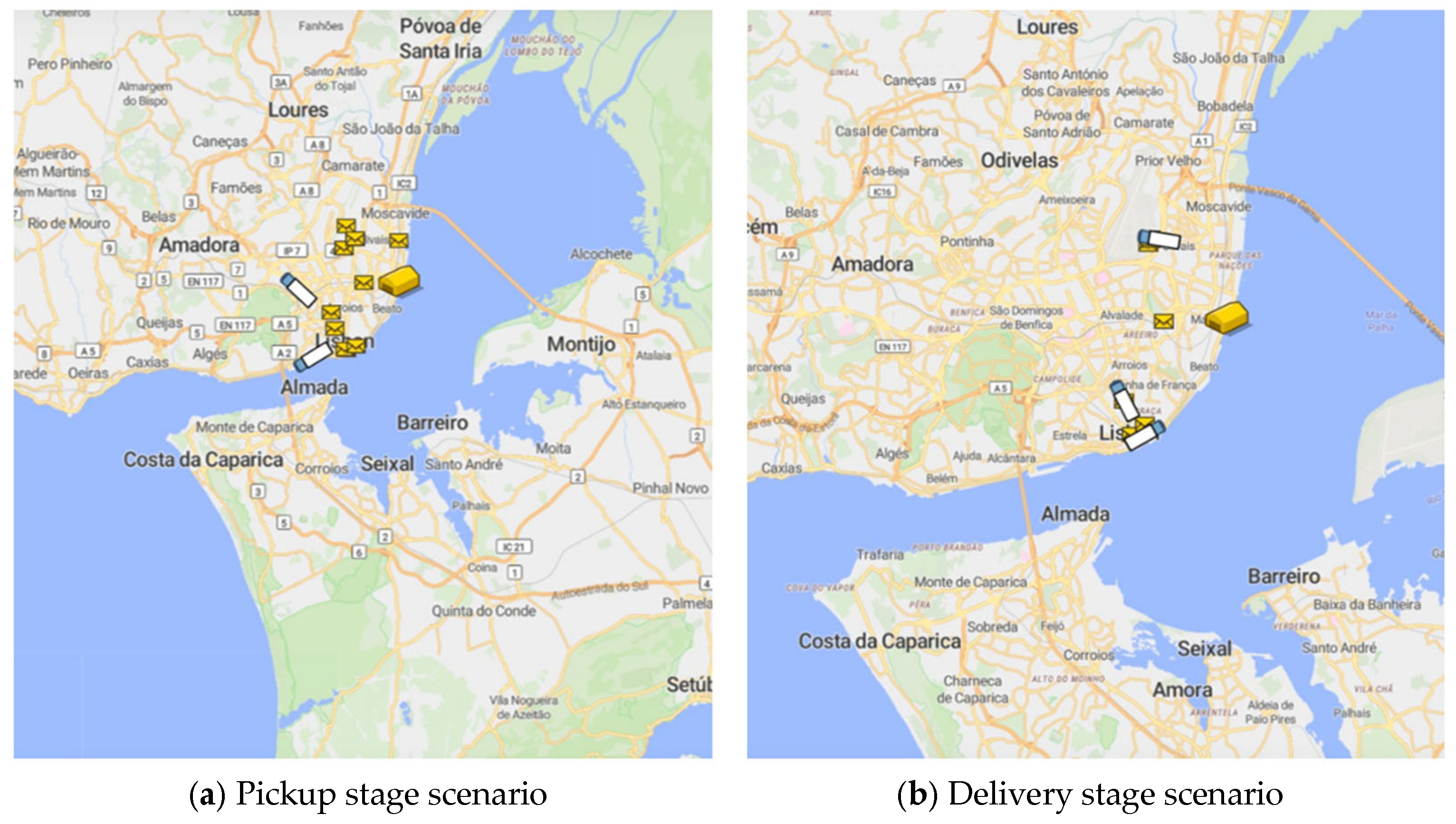
4. Case Study of Lisbon

A simulation was conducted in the city of Lisbon, Portugal. Lisbon is the largest city in the country and its capital, strategically positioned on the right bank of the Tagus River along the Atlantic coast, making it the westernmost capital of mainland Europe. Covering an area of approximately 100.05 km², Lisbon serves as the core of the Lisbon Metropolitan Area (LMA), which encompasses 18 municipalities over an area of about 3015.24 km². This metropolitan region is the most populous in Portugal, housing nearly 3 million inhabitants, representing approximately 25% of the national population, with an average population density of 956.4 inhabitants per km². Recognized as a key political, economic, and cultural hub, Lisbon plays a vital role in the integration and development of the municipalities within the LMA, including cities such as Sintra, Cascais, Almada, and Setúbal. Figure 4 illustrates the area where the simulation was applied, with a maximum permitted speed of 50 km/h incorporated into the model. Additionally, an average speed of 30 km/h was used throughout the simulation to reflect realistic driving conditions. The company operates with at least three drivers/vehicles, designated as A, B, and C, to carry out pickup and delivery tasks. The allocation of these vehicles follows the company’s predefined priority order, ensuring an optimized dispatch strategy aligned with operational preferences.

The maps in Figure 4 illustrate the spatial distribution of tasks on the day with the highest number of orders. Figure 4a shows the scenario at the pickup stage, while Figure 4b represents the delivery stage. The yellow envelope symbol corresponds to the assigned tasks, the yellow warehouse icon indicates the fixed storage unit, and the truck icons represent the drivers performing the tasks. Both views are focused on the Lisbon metropolitan area, the company’s main operating area.

The company under study operates in the cities of Lisbon and Porto, Portugal, providing flexible and on-demand baggage pickup and delivery services. However, this article focuses exclusively on the operations carried out in Lisbon. Customers can request services through various platforms, including the company’s mobile application, official website, or airline ticket booking platforms. To ensure operational efficiency, orders must be placed at least two hours in advance, allowing operators to assign tasks to available drivers.

The allocation follows a predefined priority order, with Driver A being the first choice; if unavailable, the task is reassigned to Driver B, and, if necessary, to Driver C. Additionally, orders placed one day in advance are consolidated and distributed to drivers at 7:00 AM each day, with the possibility of adjustments throughout the day, provided that the two-hour minimum lead time and priority selection criteria are respected. The operational model also considers a maximum capacity of 24 baggage volumes per vehicle, as detailed in Section 3.1.

Table 3. Historical pickup and delivery data of the company under study.

Driver Pickup–Delivery	Pickup Date	Pickup Time	Delivery Date	Delivery Time	Baggage Volume	Pickup (Latitude, Longitude)	Delivery (Latitude, Longitude)
B–A	31 December 2022	12:00	6 January 2023	18:30	8	(38.708603, 9.152313)	(38.729587, 9.145609)
B–B	5 January 2023	10:00	5 January 2023	18:00	3	(38.708603, 9.152313)	(38.768882, −9.129371)
A–A	5 January 2023	08:00	5 January 2023	15:00	3	(38.770698, −9.128416)	(38.709128, 9.131975)
B–B	5 January 2023	11:00	5 January 2023	17:00	13	(38.709886, −9.136901)	(38.768888, −9.129258)
A–A	5 January 2023	11:00	5 January 2023	17:00	5	(38.740775, −9.132096)	(38.768888, −9.129258)
A–A	5 January 2023	10:00	5 January 2023	19:00	1	(38.713089, 9.128038)	(38.763894, −9.136909)
B–B	6 January 2023	09:00	6 January 2023	15:30	3	(38.713419, −9.136630)	(38.768888, −9.129258)
B–B	6 January 2023	08:45	6 January 2023	17:30	6	(38.711479, −9.146890)	(38.768888, −9.129258)
B–B	6 January 2023	11:00	6 January 2023	18:30	2	(38.732004, −9.130959)	(38.763894, −9.136909)
A–A	6 January 2023	15:00	7 January 2023	11:00	4	(38.710027, −9.136163)	(38.768888, −9.129258)
A–A	6 January 2023	08:00	6 January 2023	16:30	2	(38.768888, −9.129258)	(38.709628, 9.135127)
A–B	6 January 2023	11:00	6 January 2023	16:30	3	(38.714964, −9.131438)	(38.768888, −9.129258)
A–A	6 January 2023	10:30	6 January 2023	17:00	3	(38.709268, 9.146129)	(38.767842, 9.099344)
B–B	6 January 2023	11:30	6 January 2023	17:00	2	(38.713236, 9.125640)	(38.775593, 9.135366)
B–B	6 January 2023	09:30	6 January 2023	18:00	2	(38.718769, −9.132179)	(38.763894, −9.136909)
A–A	6 January 2023	09:00	6 January 2023	14:00	4	(38.768990, −9.129261)	(38.711616, 9.128668)
A–A	6 January 2023	13:30	6 January 2023	17:30	4	(38.740243, −9.166652)	(38.720934, 9.143161)
C–C	7 January 2023	10:30	7 January 2023	16:00	2	(38.709903, −9.134395)	(38.763554, 9.137307)
C–C	7 January 2023	10:00	7 January 2023	18:00	3	(38.708603, 9.152313)	(38.770012, −9.128149)
A–A	7 January 2023	08:30	9 January 2023	14:30	8	(38.770698, −9.128416)	(38.768882, −9.129371)
C–B	8 January 2023	10:30	8 January 2023	18:00	9	(38.714284, −9.130639)	(38.768888, −9.129258)
C–B	8 January 2023	10:00	8 January 2023	15:30	5	(38.721265, −9.138722)	(38.770012, −9.128149)
B–B	8 January 2023	10:00	8 January 2023	16:00	3	(38.770698, −9.128416)	(38.711139, 9.135703)
B–B	9 January 2023	09:38	9 January 2023	11:45	2	(38.711377, −9.142813)	(38.785560, 9.110437)

presents a summary of the orders processed by the company within this operational framework.

To ensure the accuracy and reliability of the ABS model, a rigorous validation process was conducted. Initially, the logical consistency of the model was verified, ensuring that the Order/Task, Vehicle, and Warehouse agents accurately represented operational processes and interactions within the company studied. The behavior of each agent was analyzed to confirm its adherence to real-world system expectations. Subsequently, the model’s outputs were compared with historical company data, using a dataset of 24 orders processed between 2022 and 2023, to assess the model’s predictive alignment with observed conditions. Key Performance Indicators (KPIs), such as routing costs, completion times, and storage costs at physical locations, were evaluated to verify the consistency of the results.

Additionally, the model was validated through comparison with a well-established optimization model from the literature, where the same real-world company data were applied to the model presented in Section 3.2. This comparison allowed for an assessment of how closely the simulation results aligned with those of the optimization approach. A sensitivity analysis was also performed to examine the impact of variations in critical parameters, such as the number of available vehicles, and their effects on routing costs, storage costs, and task completion times (further detailed in the next section). Finally, the model was tested across different operational scenarios to assess its robustness and consistency, ensuring that the results generated remained reliable under varying conditions.

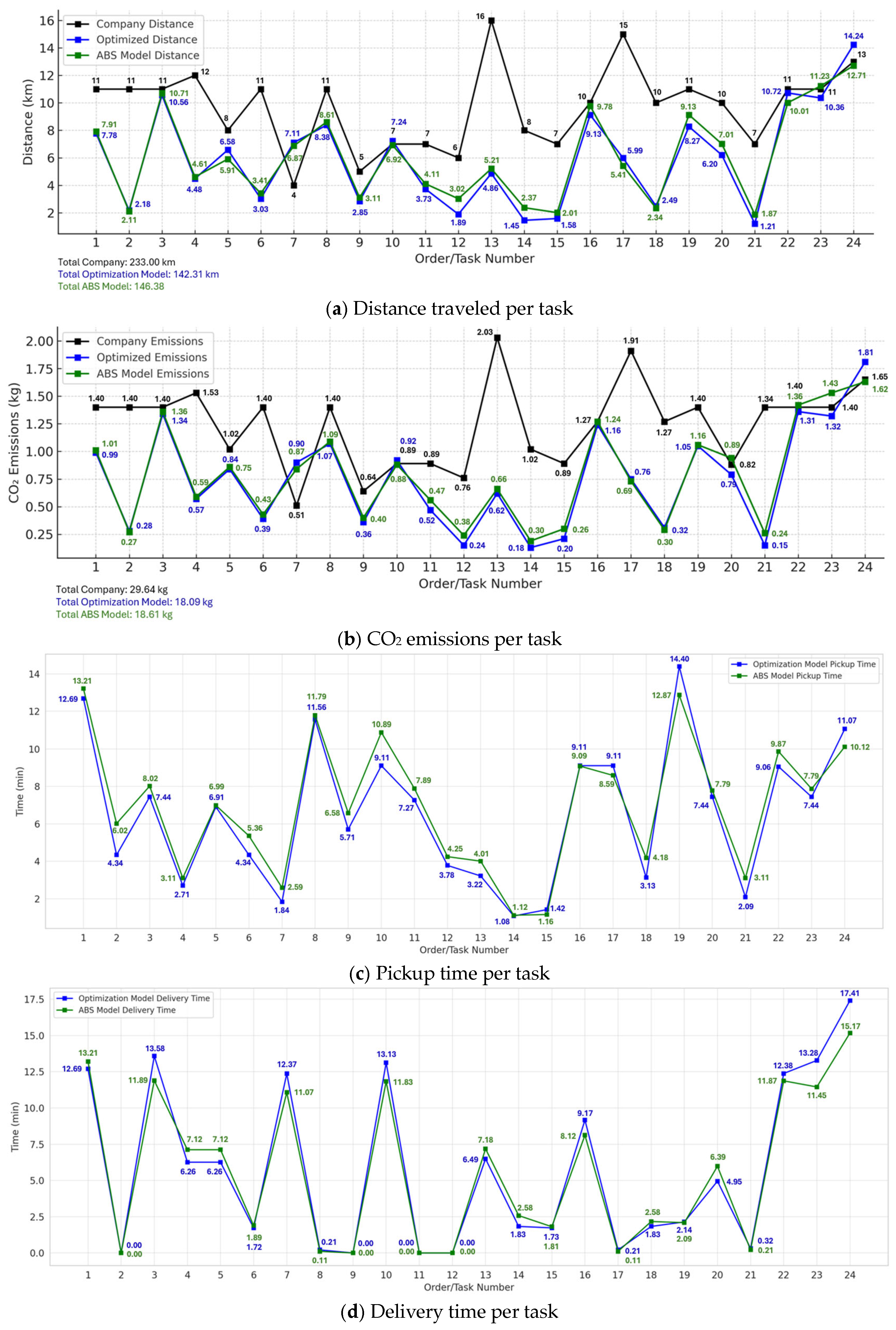
5. Results and Discussion

In this section, two different scenarios will be analyzed to evaluate the performance of the company under study’s logistics operations. Scenario 1 represents the company’s current operational model, where a simulation was conducted using 24 orders provided by the company to replicate its existing practices. This scenario enables an assessment of the current system’s efficiency by comparing real and simulated distances traveled. The cost per kilometer is estimated at approximately EUR 0.50 per km. When temporary storage in the warehouse is required, the cost for up to 24 volumes per order is EUR 5 per day, which is only used within the rules set out in Section 3.1. Scenario 2 represents the optimized scenario, determining the optimal routing and scheduling plans. The results obtained from the optimization model were then used as input parameters for the simulation model, allowing an evaluation of the optimized scenario’s behavior. In this scenario, KPIs will be analyzed, including travel time per order, distance traveled per order and in total, cost associated with travel distances, and adherence to predefined time windows. The comparative analysis between these two scenarios aims to identify opportunities for improving operational efficiency, reducing costs, and enhancing overall service performance.

5.1. Scenario 1: Current Scenario

In this first scenario, the current operational model of the company under study is analyzed, using real historical data to replicate its logistics performance. This scenario provides a benchmark for understanding the actual efficiency of the existing logistics framework by comparing real and simulated travel distances. By assessing the current scenario, KPIs such as routing efficiency, vehicle utilization, and cost implications of distance travel are examined. This allows for the identification of potential inefficiencies in the company’s operations, which will later be contrasted with the optimized scenario.

Table 4. Summary of orders and travel costs in the current scenario.

Driver Pickup–Delivery	Pickup Date/Time	Delivery Date/Time	Real Distance Traveled (KM)	ABS Model (KM)	Real Cost (EUR per KM)	ABS Model Cost (EUR per KM)	Warehouse Cost (EUR)
B–A	31 December 2022 12:00	6 January 2023 18:30	11	9.3	5.50	4.65	30.00
B–B	5 January 2023 10:00	5 January 2023 18:00	11	7.5	5.50	3.75	-
A–A	5 January 2023 8:00	5 January 2023 15:00	11	11.7	5.50	5.85	-
B–B	5 January 2023 11:00	5 January 2023 17:00	12	11.6	6.00	5.80	-
A–A	5 January 2023 11:00	5 January 2023 17:00	8	7.3	4.00	3.65	-
A–A	5 January 2023 10:00	5 January 2023 19:00	11	11.4	5.50	5.70	-
B–B	6 January 2023 9:00	6 January 2023 15:30	4	3.7	2.00	1.85	-
B–B	6 January 2023 8:45	6 January 2023 17:30	11	11.2	5.50	5.60	-
B–B	6 January 2023 11:00	6 January 2023 18:30	5	3.8	2.50	1.90	-
A–A	6 January 2023 15:00	7 January 2023 11:00	7	6.3	3.50	3.15	5.0
A–A	6 January 2023 8:00	6 January 2023 16:30	7	5.7	3.50	2.85	-
A–B	6 January 2023 11:00	6 January 2023 16:30	6	4.8	3.00	2.40	-
A–A	6 January 2023 10:30	6 January 2023 17:00	16	19.8	8.00	9.90	-
B–B	6 January 2023 11:30	6 January 2023 17:00	8	6.7	4.00	3.35	-
B–B	6 January 2023 9:30	6 January 2023 18:00	7	3.3	3.50	1.65	-
A–A	6 January 2023 9:00	6 January 2023 14:00	10	8.8	5.00	4.40	-
A–A	6 January 2023 13:30	6 January 2023 17:30	15	18.4	7.50	9.20	-
C–C	7 January 2023 10:30	7 January 2023 16:00	10	7.7	5.00	3.85	-
C–C	7 January 2023 10:00	7 January 2023 18:00	11	9.8	5.50	4.90	-
A–A	7 January 2023 8:30	9 January 2023 14:30	10	9.6	5.00	4.80	10.00
C–B	8 January 2023 10:30	8 January 2023 18:00	7	8.5	3.50	4.25	-
C–B	8 January 2023 10:00	8 January 2023 15:30	11	11.9	3.50	5.95	-
B–B	8 January 2023 10:00	8 January 2023 16:00	11	12.3	5.50	6.15	-
B–B	9 January 2023 9:38	9 January 2023 11:45	13	12.7	6.50	6.35	-

presents the details of the orders considered, listing essential attributes such as the assigned driver, pickup and delivery times, baggage volume, travel distance (both real and simulated), and associated costs (i.e., transportation and warehouse expenses).

Moreover, the comparison of routing costs reveals that, in most cases, the simulated cost per kilometer is slightly lower than the real cost, suggesting opportunities for route optimization. For instance, in the order assigned to Driver A on 6 January 2023 at 10:30, the company recorded 16 km, whereas the simulation carried out the route to 19.8 km, highlighting possible real-world constraints such as traffic conditions, driver route preferences, or suboptimal path selection. Additionally, the role of warehouse storage in certain deliveries underscores the need for dynamic fleet management. Some orders required temporary storage due to scheduling constraints, leading to additional costs, such as EUR 5.00 on 6 January 2023 and EUR 10.00 on 7 January 2023. These findings emphasize that optimizing vehicle allocation strategies and minimizing reliance on storage facilities could further enhance cost efficiency. Overall, the current scenario simulation effectively replicates the company’s real-world operations, providing a strong baseline for comparison with the optimized scenario, where further improvements in routing efficiency, cost reduction, and resource allocation will be examined.

5.2. Scenario 2: Optimal Scenario

Scenario 2 represents the optimized operational model, where the PDP-TW model, adapted from Lyu and Yu [6], was tailored to fit the specifics of this study. The optimization model was implemented in Julia 1.10.5, using the JuMP library for mathematical formulation and Gurobi 11.0.3 to solve the problem, running on an Intel Core i5-8265U 1.60 GHz with 20 GB of RAM with default parameters on a single thread. The mathematical model was executed for the analyzed instances until the optimal solution was found. For the instances corresponding to 31 December, 5 January, 6 January, 7 January, 8 January, and 9 January, the execution time required to obtain the optimal solution was, respectively, 0.31, 0.37, 4.34, 0.21, 0.03, and 0.03 s.

The results were then used as input data for the ABS model, allowing a comparative analysis between the current operational scenario (Scenario 1) and the optimized scenario (Scenario 2), as well as between the optimal results from the PDP-TW optimization model and the corresponding ABS model outcomes. This comparison assesses the proximity between the results and examines whether the time window constraints were met in both models. However, it is important to note that, even in the optimized scenario simulation, uncertainty factors such as traffic variations and unforeseen delays are not yet considered, as the ABS model remains deterministic.

Table 5. Optimized scenario: PDP-TW results from the optimization model vs. ABS model.

Real Order Pickup Date/Time	Real Order Delivery Date/Time	Company Distance (KM)	Optimization Optimal Distance (KM)	ABS Model Optimal Distance (KM)	Real Cost (EUR per KM)	Optimized Cost (EUR per KM)	ABS Model Optimal Cost (EUR per KM)	Optimized Time (Pickup—Delivery)	ABS Time (Pickup—Delivery)	Time Window Adherence (Optimization/Simulation)	Warehouse Usage (Yes/No)
31 December 2022 12:00	6 January 2023 18:30	11	7.78	7.91	5.50	3.89	3.96	10:50–18:20	10:48–18:26	Yes—Yes	Yes
5 January 2023 10:00	5 January 2023 18:00	11	2.18	2.11	5.50	1.09	1.06	10:00–17:50	09:57–17:59	Yes—Yes	No
5 January 2023 08:00	5 January 2023 15:00	11	10.56	10.71	5.50	5.28	5.36	08:10–14:50	08:12–14:57	Yes *—Yes *	No
5 January 2023 11:00	5 January 2023 17:00	12	4.48	4.61	6.00	2.24	2.31	10:57–16:50	11:02–17:01	Yes—Yes *	No
0 January 2023 11:00	5 January 2023 17:00	8	6.58	5.91	4.00	3.29	2.96	11:00–16:50	11:17–16:55	Yes—Yes	No
5 January 2023 10:00	5 January 2023 19:00	11	3.03	3.41	5.50	1.52	1.71	09:55–18:50	09:59–18:58	Yes—Yes	No
6 January 2023 09:00	6 January 2023 15:30	4	7.11	6.87	2.00	3.56	3.44	08:50–15:20	09:04–15:28	Yes—Yes	No
6 January 2023 08:45	6 January 2023 17:30	11	8.38	8.61	5.50	4.19	4.31	08:45–17:20	08:45–17:26	Yes—Yes	No
6 January 2023 11:00	6 January 2023 18:30	5	2.85	3.11	2.50	1.43	1.56	10:50–18:30	11:00–18:36	Yes—Yes *	No
6 January 2023 15:00	7 January 2023 11:00	7	7.24	6.92	3.50	3.62	3.46	14:50–10:50	14:54–11:00	Yes—Yes	Yes
6 January 2023 08:00	6 January 2023 16:30	7	3.73	4.11	3.50	1.87	2.06	08:10–16:20	08:17–16:27	Yes—Yes	No
6 January 2023 11:00	6 January 2023 16:30	6	1.89	3.02	3.00	0.95	1.51	10:53–16:20	10:59–16:30	Yes—Yes	No
6 January 2023 10:30	6 January 2023 17:00	16	4.86	5.21	8.00	2.43	2.61	10:20–17:00	10:28–17:03	Yes—Yes *	No
6 January 2023 11:30	6 January 2023 17:00	8	1.45	2.37	4.00	0.73	1.19	11:20–16:50	11:24–16:59	Yes—Yes	No
6 January 2023 09:30	6 January 2023 18:00	7	1.58	2.01	3.50	0.79	1.01	09:20–17:50	09:27–18:03	Yes—Yes *	No
6 January 2023 09:00	6 January 2023 14:00	10	9.13	9.78	5.00	4.57	4.89	08:50–13:50	08:58–13:59	Yesc– Yes	No
6 January 2023 13:30	6 January 2023 17:30	15	5.99	5.41	7.50	3.00	2.71	13:20–17:20	13:30–17:29	Yes—Yes	No
7 January 2023 10:30	7 January 2023 16:00	10	2.49	2.34	5.00	1.25	1.17	10:20–15:50	10:27–15:59	Yes—Yes	No
7 January 2023 10:00	7 January 2023 18:00	11	8.27	9.13	5.50	4.14	4.57	09:50–17:50	09:57–18:00	Yes—Yes	No
7 January 2023 08:30	9 January 2023 14:30	10	6.20	7.01	5.00	3.10	3.51	08:20–14:30	08:30–14:29	Yes—Yes	Yes
8 January 2023 10:30	8 January 2023 18:00	7	1.21	1.87	3.50	0.61	0.94	10:20–17:50	10:29–18:00	Yes—Yes	No
8 January 2023 10:00	8 January 2023 15:30	11	10.72	10.01	3.50	5.36	5.01	09:50–15:20	09:52–15:29	Yes—Yes	No
8 January 2023 10:00	8 January 2023 16:00	11	10.36	11.23	5.50	5.18	5.62	09:50–15:50	09:50–15:59	Yes—Yes	No
9 January 2023 09:38	9 January 2023 11:45	13	14.24	12.71	6.50	7.12	6.36	09:28–11:35	09:30–11:41	Yes—Yes	No

* It meets the time window as it is within the 10 min tolerance.

presents the optimized results, detailing the differences between the optimal values obtained in the PDP-TW optimization model and their respective simulated values in the ABS model. This comparison provides insights into the potential efficiency gains and highlights any deviations that may occur when transitioning from an optimized theoretical model to a realistic ABS model.

In Table 5, the comparative analysis between the PDP-TW models, Optimization and the ABS, respectively, demonstrated significant proximity between the results. The total operational distance recorded by the company was 233 km, whereas the optimized model resulted in 142.31 km, and the ABS model of the optimized scenario reached 146.38 km. Similarly, cost values followed the same trend, with the company’s real cost totaling EUR 116.50, while the optimized model and ABS model yielded EUR 71.21 and EUR 73.29, respectively. These results reinforce the effectiveness of combining optimization and ABS methodologies in reducing travel distance and costs, providing a more efficient alternative to the company’s current operations.

However, it is important to emphasize that while the optimization model successfully adhered to all time window constraints, one delivery occurred exactly at the limit of the pre-established 10 min tolerance. In contrast, the ABS model also respected all time windows constraints, but in five instances, the deliveries were completed within this same 10 minc margin. Although these results do not constitute violations, they indicate proximity to the operational threshold. This reinforces the model’s reliability under deterministic assumptions but also suggests potential areas for refinement in real-world applications. Therefore, the optimized task allocation and routing strategies effectively minimized inefficiencies, while future improvements could focus on enhancing time buffer management to further strengthen compliance with delivery schedules. A promising direction in PDP-TW research involves incorporating uncertainty into optimization models, a feature more naturally handled by ABS approaches. Recent studies [10,16,17,19,27] highlight this evolution. Future work should critically explore this integration to improve realism and robustness in urban logistics planning.

Finally, an estimation of the CO₂ is analyzed for each scenario. The estimation was based on fuel consumption and emission factors commonly reported in the literature. For diesel-powered vehicles, an average fuel consumption of 0.041 L/km, in combination with an emission factor of 3.1 kg CO₂ per liter of diesel, as reported by Armenta-Déu [28], who evaluated the environmental impact of urban transportation across different driving modes and fuel types. By multiplying the consumption rate by the emission factor, a composite value of 0.1271 kg CO₂ per kilometer was obtained. Figure 5 presents the main performance indicators analyzed across the three operational scenarios: the company’s real-world execution, the optimal routing derived from the optimization model, and the corresponding scenario simulated using the ABS model. Each individual order is associated with a specific travel distance, estimated CO₂ emissions, and travel time. These metrics are displayed per task, enabling a detailed comparison of operational efficiency and environmental impact among the three approaches.

Figure 5 presents a detailed comparison of KPIs across the three operational scenarios analyzed: the company’s real-world operations, the optimal solution generated by the optimization model, and the simulation of this optimized solution using the ABS model. The evaluated KPIs include distance traveled, CO₂ emissions, travel time (pickup and delivery), vehicle capacity utilization, number of vehicles used, and time window adherence.

In terms of distance traveled (Figure 5a), both the optimization and ABS models significantly reduced the total distance compared to the company’s static routing strategy. This reduction directly impacts CO₂ emissions (Figure 5b), which serve as a critical indicator of environmental performance. The company’s operations resulted in substantially higher emissions (29.64 kg), while the optimized scenario and its ABS yielded lower emissions—18.09 kg and 18.61 kg, respectively. These results reinforce the environmental benefits of efficient route planning and dynamic task assignment.

The analysis of travel time per task (Figure 5c,d) reveals consistency between the optimization and ABS models, further validating the simulation’s ability to replicate optimized outcomes. Additionally, the company required three drivers to complete the deliveries, while the optimized scenario used two, indicating improved vehicle allocation and suggesting better resource utilization. Regarding capacity utilization, none of the deliveries exceeded the vehicle’s limit of 24 volume units, although several tasks operated at full capacity, highlighting effective load management under optimized conditions.

Finally, time window adherence was respected in all three scenarios. However, while the optimization model had one delivery completed at the exact limit of the 10 min tolerance, the ABS had five deliveries under similar conditions, signaling proximity to the threshold but still within acceptable operational performance.

A key finding is that, unlike the current scenario (Scenario 1), where three drivers were used, the optimized scenario (both in the optimization model and ABS model) required a maximum of only two drivers, demonstrating that a third driver was unnecessary for the given set of orders. The results suggest that the heuristic procedure currently employed by the company for driver assignment may be suboptimal, even under limited task volumes. This suboptimality, if not addressed, has the potential to scale disproportionately with increasing operational complexity, leading to elevated costs and reduced efficiency. Consequently, a restructuring of the company’s driver allocation strategy is warranted. This could be achieved either through the implementation of mathematical optimization models or the adoption of more effective heuristic approaches that are rigorously evaluated using ABS. Such integration is expected to enhance the utilization of available resources and improve the overall cost-effectiveness of urban logistics operations. Additionally, the current driver prioritization rule—which first assigns tasks to Driver A, then to B, and finally to C was not followed in the optimized model, where assignments were based solely on minimizing total distance. This further highlights the need for a more flexible tasking approach, where efficiency takes precedence over driver prioritization.

Another important aspect is the cost structure considered in this study. The final service cost of the company includes multiple variables—such as airport fees and out-of-zone travel charges, which were not available for analysis. Instead, the study focused on two measurable cost components: the cost per kilometer traveled and warehouse storage costs, which were EUR 5 per day for up to 24 volumes. Additionally, it is crucial to note that the cost values presented in Table 5 are directly linked to the respective orders, meaning that the distances traveled by drivers when returning to the warehouse were not included unless they were directly related to storage needs. This occurred in three cases, where deliveries required temporary warehouse storage.

From a sustainability perspective, reducing travel distances directly contributes to lowering CO₂ emissions, as the company’s fleet consists of non-electric vehicles. The company’s original operations covered 233 km, whereas the optimized scenario reduced this by approximately 38%, leading to substantial fuel savings and emission reductions. This reinforces the environmental benefits of integrating optimization and ABS methodologies, aligning logistics efficiency with sustainable transportation practices. Additionally, the ABS assumed a fixed speed of 30 km/h, reflecting urban traffic conditions in Lisbon, where speed limits and frequent stops influence delivery times. While this assumption provides a reasonable approximation, future enhancements could incorporate dynamic speed adjustments based on real-time traffic data, further improving the model’s accuracy. These insights validate the integrated modeling approach, illustrating how optimization and ABS can complement each other to assess and enhance urban logistics efficiency from both operational and sustainability perspectives, reinforcing the importance of data-driven decision-making in logistics.

5.3. Limitations

While the developed ABS model has proven effective in replicating the company’s logistics operations and facilitating a comparative analysis with the optimization-based PDP-TW model, certain limitations should be acknowledged. First, the dataset used in this study consisted of 24 orders, which was sufficient for the development and validation of the ABS model and its comparison with the optimization model. However, for future research, it is recommended to increase the dataset and vary the number of available drivers to better analyze the impact on model performance and scalability. Additionally, the ABS model currently operates in a deterministic framework, meaning that uncertainty factors such as traffic conditions and unforeseen delays have not yet been incorporated. Future enhancements will include stochastic elements to better reflect real-world conditions. Another limitation is the fixed average speed of 30 km/h used in the ABS model, which, while suitable for simulating urban logistics in Lisbon, could be further refined by integrating dynamic speed variations based on traffic patterns. Despite these limitations, the developed ABS model provides a strong foundation for evaluating operational efficiency and serves as a valuable tool for future improvements, where additional refinements will enhance its applicability in complex, real-world logistics environments.

6. Conclusions and Future Research

This study applied an ABS model and an optimization approach to analyze real-world PDP-TW in urban logistics. The research focused on comparing the company’s current operational scenario with an optimized scenario generated using a PDP-TW mathematical model. The integration of optimization and ABS model enabled a comparative analysis of KPIs defined in the conceptual model, including total traveled distance, service time, number of vehicles used, warehouse usage, time window adherence, and CO₂ emissions.

The results demonstrated that the optimized scenario significantly reduced the total traveled distance from 233 km to 142.31 km in the optimization model and 146.38 km in the ABS of the optimized scenario. Likewise, the total operational cost decreased from EUR 116.50 to EUR 71.21 and EUR 73.29, respectively. The estimated CO₂ emissions, derived from diesel fuel consumption, dropped from 29.64 kg in the real-world operations to 18.09 kg in the optimized model and 18.61 kg in the ABS model, emphasizing the environmental benefits of route optimization. These findings validate the effectiveness of the optimization model in improving efficiency and confirm the ABS model’s ability to approximate optimal outcomes in a deterministic setting.

Despite the operational improvements, all deliveries complied with the time windows; however, the proximity of some to the pre-established 10 min tolerance, one in the optimization model and five in the ABS model, highlights the need for refined scheduling strategies and improved time buffer management. Furthermore, only two drivers were required in the optimized scenario compared to three in the real operation, suggesting that current fleet deployment can be improved. While this study offers important insights, certain limitations must be acknowledged. The simulation was conducted using a dataset of 24 orders, which was sufficient for initial validation purposes but may not capture the full scope of operational variability. Furthermore, the current ABS model operates under deterministic assumptions and does not incorporate real-world uncertainties such as traffic congestion, vehicle breakdowns, or unexpected delays. Future research should consider the integration of stochastic parameters, expansion of the dataset, and implementation of adaptive routing mechanisms to enhance both robustness and realism in logistical planning. In particular, the inclusion of uncertainty within the ABS framework will be crucial to significantly improve its representational accuracy and decision-support capabilities in complex urban logistics environments.

References

1. Goetz, A.R. Transport Challenges in Rapidly Growing Cities: Is There a Magic Bullet? Transp. Rev. 2019, 39, 701–705. [Google Scholar] [CrossRef]
2. Moreno, R.P.; Lopes, R.B.; Ferreira, J.V.; Ramos, A.L.; Correia, D. A Study of the Main Mathematical Models Used in Mobility, Storage, Pickup and Delivery in Urban Logistics: A Systematic Review. Systems 2024, 12, 374. [Google Scholar] [CrossRef]
3. Lagorio, A.; Pinto, R.; Golini, R. Research in Urban Logistics: A Systematic Literature Review. Int. J. Phys. Distrib. Logist. Manag. 2016, 46, 908–931. [Google Scholar] [CrossRef]
4. Frederhausen, S.; Klumpp, M. Commercial Electric Vehicle Routing in Urban Logistics: A Systematic Literature Review. In Data Science in Maritime and City Logistics: Data-driven Solutions for Logistics and Sustainability. Proceedings of the Hamburg International Conference of Logistics (HICL); Jahn, C., Kersten, W., Ringle, C.M., Eds.; epubli GmbH: Berlin, Germany, 2020; Volume 30, pp. 33–69. [Google Scholar]
5. Mitrović-Minić, S.; Laporte, G. The Pickup and Delivery Problem with Time Windows and Transshipment. INFOR 2006, 44, 217–227. [Google Scholar] [CrossRef]
6. Lyu, Z.; Yu, A.J. The Pickup and Delivery Problem with Transshipments: Critical Review of Two Existing Models and a New Formulation. Eur. J. Oper. Res. 2023, 305, 260–270. [Google Scholar] [CrossRef]
7. Wolfinger, D. A Large Neighborhood Search for the Pickup and Delivery Problem with Time Windows, Split Loads and Transshipments. Comput. Oper. Res. 2021, 126, 105110. [Google Scholar] [CrossRef]
8. Min, H. The Multiple Vehicle Routing Problem with Simultaneous Delivery and Pick-up Points. Transp. Res. Part Gen. 1989, 23, 377–386. [Google Scholar] [CrossRef]
9. Martinez, L.M.; Correia, G.H.A.; Viegas, J.M. An Agent-Based Simulation Model to Assess the Impacts of Introducing a Shared-Taxi System: An Application to Lisbon (Portugal). J. Adv. Transp. 2015, 49, 475–495. [Google Scholar] [CrossRef]
10. Murarețu, I.; Bădică, C. Optimal Agent-Based Pickup and Delivery with Time Windows and Electric Vehicles. Appl. Sci. 2024, 14, 7528. [Google Scholar] [CrossRef]
11. Mehdizadeh, M.; Nordfjaern, T.; Klöckner, C.A. A Systematic Review of the Agent-Based Modelling/Simulation Paradigm in Mobility Transition. Technol. Forecast. Soc. Chang. 2022, 184, 122011. [Google Scholar] [CrossRef]
12. Rao, C.; Goh, M.; Zhao, Y.; Zheng, J. Location Selection of City Logistics Centers under Sustainability. Transp. Res. Part Transp. Environ. 2015, 36, 29–44. [Google Scholar] [CrossRef]
13. Anily, S.; Hassin, R. The Swapping Problem. Networks 1992, 22, 419–433. [Google Scholar] [CrossRef]
14. Santos, D.O.; Xavier, E.C. Taxi and Ride Sharing: A Dynamic Dial-a-Ride Problem with Money as an Incentive. Expert Syst. Appl. 2015, 42, 6728–6737. [Google Scholar] [CrossRef]
15. Tadei, R.; Perboli, G.; Ricciardi, N.; Baldi, M.M. The Capacitated Transshipment Location Problem with Stochastic Handling Utilities at the Facilities. Int. Trans. Oper. Res. 2012, 19, 789–807. [Google Scholar] [CrossRef]
16. Abreu, A.P. The Robust Pickup and Delivery Problem with Time Windows. Master’s Thesis, Federal University of São Carlos, São Carlos, Brazil, 2025. [Google Scholar]
17. Khanna, A.; Liu, F.; Gupta, S.; Pavia, S.; Mukhopadhyay, A.; Dubey, A. PDPTW-DB: MILP-Based Offline Route Planning for PDPTW with Driver Breaks. In Proceedings of the 26th International Conference on Distributed Computing and Networking, Hyderabad, India, 4–7 January 2025; pp. 73–83. [Google Scholar]
18. Dridi, I.H.; Kammarti, R.; Ksouri, M.; Borne, P. Genetic Algorithm for Mulicriteria Optimization of a Multi-Pickup and Delivery Problem with Time Windows. In Proceedings of the 13th IFAC Symposium on Information Control Problems in Manufacturing: Moscow, Russia, 3–5 June 2009; Volume 42, pp. 1538–1543. [Google Scholar] [CrossRef]
19. Ma, Y.; Yang, L.; Li, Z.; Lev, B. An Adaptive Genetic Algorithm with Neighborhood Search for Integrated O2O Takeaway Order Assignment and Delivery Optimization by E-Bikes with Varied Compartments. Appl. Soft Comput. 2024, 167, 112277. [Google Scholar] [CrossRef]
20. Helo, P.; Rouzafzoon, J. An Agent-Based Simulation and Logistics Optimization Model for Managing Uncertain Demand in Forest Supply Chains. Supply Chain Anal. 2023, 4, 100042. [Google Scholar] [CrossRef]
21. Karney, C.F.F. Algorithms for Geodesics. J. Geod. 2013, 87, 43–55. [Google Scholar] [CrossRef]
22. AnyLogic: Simulation Modeling Software Tools & Solutions for Business. Available online: https://www.anylogic.com/ (accessed on 5 April 2025).
23. Miller, C.E.; Tucker, A.W.; Zemlin, R.A. Integer Programming Formulation of Traveling Salesman Problems. J. ACM 1960, 7, 326–329. [Google Scholar] [CrossRef]
24. Attajer, A.; Darmoul, S.; Chaabane, S.; Riane, F.; Sallez, Y. Benchmarking Simulation Software Capabilities Against Distributed Control Requirements: FlexSim vs. AnyLogic. In Service Oriented, Holonic and Multi-Agent Manufacturing Systems for Industry of the Future; Borangiu, T., Trentesaux, D., Leitão, P., Cardin, O., Lamouri, S., Eds.; Springer International Publishing: Cham, Germany, 2021; pp. 520–531. [Google Scholar]
25. Hussein, M.; Karam, A.; Eltoukhy, A.E.E.; Darko, A.; Zayed, T. Optimized Multimodal Logistics Planning of Modular Integrated Construction Using Hybrid Multi-Agent and Metamodeling. Autom. Constr. 2023, 145, 104637. [Google Scholar] [CrossRef]
26. Abdelmageed, S.; Abdelkhalek, S.; Hussien, M.; Zayed, T. A Hybrid Simulation Model for Modules Installation in Modular Integrated Construction Projects. Int. J. Constr. Manag. 2024, 24, 1407–1418. [Google Scholar] [CrossRef]
27. Santiyuda, G.; Wardoyo, R.; Pulungan, R.; Yu, V.F. Multi-Objective Reinforcement Learning for Bi-Objective Time-Dependent Pickup and Delivery Problem with Late Penalties. Eng. Appl. Artif. Intell. 2024, 128, 107381. [Google Scholar] [CrossRef]
28. Armenta-Déu, C. Environmental Impact of Urban Surface Transportation: Influence of Driving Mode and Drivers’ Attitudes. Pollutants 2025, 5, 5. [Google Scholar] [CrossRef]
Figure 1. Flowchart of the conceptual model to be simulated.
Asi 08 00066 g001
Figure 2. An illustrative example of the PDP-TW.
Asi 08 00066 g002
Figure 3. Task execution and vehicle dispatch flow in the ABS.
Asi 08 00066 g003
Figure 4. Simulation area and route analysis for pickup and delivery operations.
Asi 08 00066 g004
Figure 5. Comparative analysis of distancec, CO2 emissions, and travel time per task across operational scenarios.
Asi 08 00066 g005