Abstract
We study the throughput and losses of a buffer with stochastically dependent service times. Such dependence occurs not only in packet buffers within TCP/IP networks but also in many other queuing systems. We conduct a comprehensive, time-dependent analysis, which includes deriving formulae for the count of packets processed and lost over an arbitrary period, the temporary intensity of output traffic, the temporary intensity of packet losses, buffer throughput, and loss probability. The model considered enables mimicking any packet interarrival time distribution, service time distribution, and correlation between service times. The analytical findings are accompanied by numerical computations that demonstrate the influence of various factors on buffer throughput and losses. These results are also verified through simulations.
1. Introduction
Traffic in TCP/IP networks often exhibits a stochastically intra-dependent structure on several levels. Perhaps the most notable observed dependence is the dependence of packet interarrival intervals, discovered 30 years ago by Leland et al. [1]. Since then, hundreds of articles have been disseminated on the impact of this dependence on the performance of packet buffers in network nodes. In particular, various performance metrics have been derived based on different intra-dependent traffic models and other assumptions.
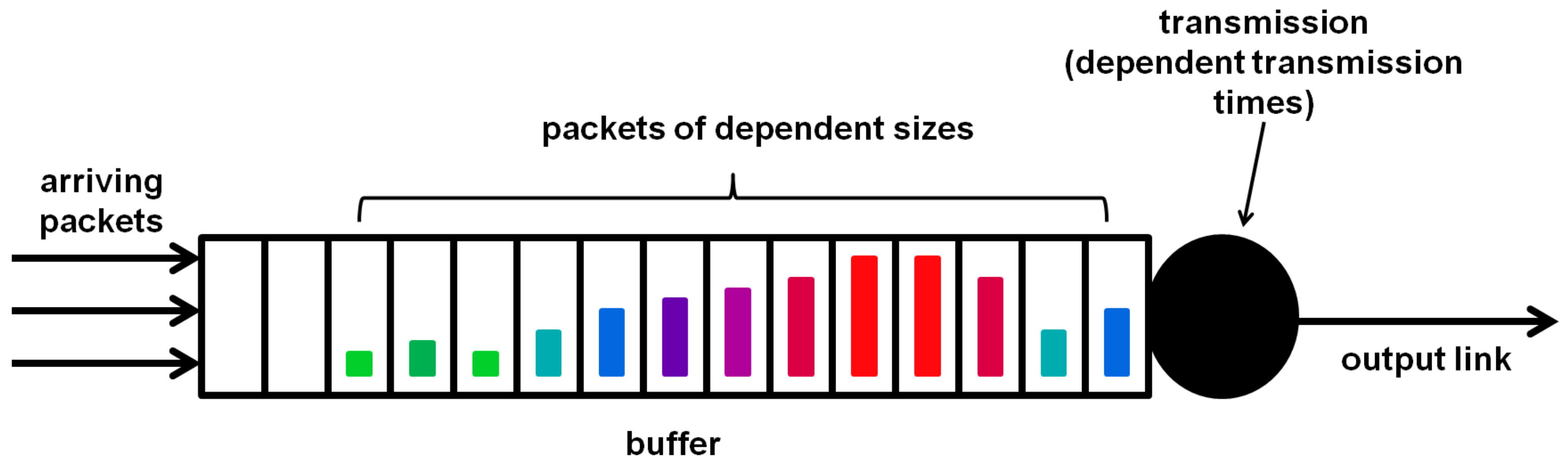
Another significant dependence in TCP/IP traffic is the stochastic dependence of consecutive packet sizes (see, e.g., [2]). Such dependent packet sizes, illustrated in various colors in Figure 1, translate into dependent transmission times, because the packet transmission time is usually proportional to its size.
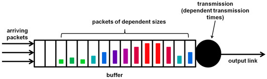
Figure 1.
Packet buffer with stochastically dependent packet sizes and service times.
The literature on buffers with stochastically dependent service times is much more limited compared to that on buffers with dependent interarrival intervals. It mainly focuses on the stationary analysis of a few basic characteristics, such as queue size and sojourn time (more details will be provided in the next section).
In this paper, we conduct a comprehensive analysis of the throughput-related characteristics of a buffer model with dependent service times and finite buffer capacity. Specifically, we derive formulae for the count of packets processed and lost over an arbitrary interval, the time-dependent output traffic intensity, throughput and loss probability, and the time-dependent loss intensity. Naturally, all throughput-related characteristics are especially important from a networking perspective, where they constitute crucial performance metrics in addition to queueing-induced delay.
The queuing model considered consists of a renewal input process with general distribution of the time intervals between consecutive packets. The consecutive packet transmission times are modeled using a Markovian service process. This service model combines analytical accessibility with the ability to model any real service time distribution with arbitrary precision and to mimic any correlation function of service times. Additionally, a finite buffer is considered, which is essential given real networking buffers and packet losses resulting from buffer overflows.
In addition to theorems and formulae, a set of numerical examples is presented. Rather than using fixed arrival and service processes, we consider a class of arrival processes and a class of service processes in these examples, with continuously increasing standard deviation of the interval between arrivals and continuously increasing correlation coefficients of service times. We demonstrate how these features influence throughput-related characteristics in both time-dependent and stationary cases. Finally, the analytical results are validated using discrete-event simulations performed in the OMNeT++ environment [3].
In detail, the key contributions of this article consist of the following:
- (a)
- A theorem on the expected count of packets processed in (Theorem 1);
- (b)
- A formula on the output traffic intensity at t (Corollary 1);
- (c)
- A formula for the buffer throughput (Corollary 2);
- (d)
- A theorem on the expected count of lost packets in (Theorem 2);
- (e)
- A formula on the loss intensity at t (Corollary 3);
- (f)
- A formula for the overall loss probability (Corollary 4).
Finally, it should be underlined that the goal of this paper is not to study a precise model of TCP/IP traffic and its interaction with the buffer. Such a model would have to incorporate other features of traffic that are not present in this paper. The main purpose of this paper is to study how the dependence of service times influences the buffer throughput. Therefore, for instance, the correlation of interarrival times—which is also present in TCP/IP traffic and certainly influences the throughput—is intentionally omitted. Including multiple factors, each of which causes the degradation of the throughput, would make it difficult to separate the impact of each factor. More on the behavior of TCP/IP flows in a limited buffer can be found, e.g., in [4,5,6,7,8,9], while more on the precise modeling of TCP/IP traffic can be found in, e.g., [10,11,12,13].
The rest of this study is laid out as follows. Section 2 provides an overview of related works on queueing models with Markovian service processes. In Section 3, we specify the buffer and traffic model of interest. Section 4 presents the derivation of the formulae for throughput-related characteristics, as outlined in points (a)–(c) above. In Section 5, we derive the formulae for loss-related characteristics, as listed in points (d)–(f) above. Numerical examples are provided in Section 6. Finally, concluding remarks are presented in Section 7.
2. Related Works
Based on the author’s information, the results shared here are novel, including all the theorems and corollaries listed in points (a)–(f) of the previous section, as well as all the numerical examples in Section 6. The previous studies, mentioned in the next paragraph, focus solely on the stationary analysis and do not address the throughput of the buffer.
The first article in which dependent service times of a queueing system are modeled in the Markovian service process is [14]. The interarrival times constitute a renewal process in [14], meaning they are independent and identically distributed, with an arbitrary interarrival distribution of finite mean. The buffer capacity is finite. For such a model, the stationary queue size distribution is obtained in [14]. To achieve this, the classic method of using a supplementary variable and calculating the stationary distribution of the embedded Markov chain is utilized. In [15], the tail of this distribution, but for a model with an infinite buffer, was investigated. In [16], other characteristics were studied, including the queue size at arrival epochs and the response time, for both finite and infinite buffer models. Ref. [17] is devoted to a multi-server model with a finite buffer, where the queue length and busy period distributions are derived. In [18], the queue size and queuing delay distributions are investigated under a slightly different service process, in which after an idle period, service always begins with a given phase distribution. In [19], a model with a finite buffer and group arrivals is considered, with two possible group acceptance protocols (total group rejection and partial group rejection). The queue size distribution, queuing delay distribution, and blocking probability of the last and first jobs in a group are obtained. Ref. [20] deals with an infinite-buffer model involving group services, where the queue length distribution and response time are computed. Ref. [21] demonstrates a different method of solving a model with an infinite buffer by exploiting the characteristic equation and its roots. In [22], the response time and inter-departure interval correlation are investigated in a model with an infinite buffer. Refs. [23,24] analyze a model with an infinite buffer and group arrivals. Specifically, Ref. [23] focuses on the queue length, busy period, and idle period, while [24] is devoted to the queuing delay distribution. Reference [25] also focuses on a group-arrival model but with a finite buffer. In [26], a model with a finite buffer and group service is revisited, with the analysis focusing on optimizing the system’s profit by maximizing a utility function composed of several performance metrics. Lastly, in [27], two models of group servicing are compared: in one model, the service phase remains unchanged during the system’s idle period, while in the other, the service phase evolves continuously, including during idle periods.
It should also be stressed that a different method is used in this paper than in [14,15,16,17,18,19,20,21,22,23,24,25,26,27]. The method here is based on solving the system of integral equations in the Laplace transform domain using a special recurrent sequence. The great advantage of this method is that it provides both the time-dependent and stationary solutions simultaneously. The classic approach used in the previous works is based on the analysis of embedded Markov chains and allows for obtaining only the stationary characteristics.
There is only one recently published study that provides a full, time-dependent analysis of a model with a finite buffer [28]. However, it is devoted solely to queue size, with no investigation of throughput-related characteristics.
3. Buffer Model
We consider a packet buffer in which a queue of packets waiting for transmission is stored. The queue is emptied from the front in FIFO manner, while the service (transmission) times of packets are mutually dependent and follow Markovian service process [16]. The description of the Markovian service process requires an underlying phase process, , with the space of possible phases , and two matrices, and . Moreover, has negative elements on the diagonal and non-negative elements off the diagonal, whereas is non-negative and is a transition-rate matrix.
During a busy period, the phase process evolves exactly as a continuous-time Markov process with transition-rate matrix . Moreover, if at some t during a busy period, then at , the phase may switch to j with probability , and the current packet transmission is continued, or the phase may switch to j with probability , and the current packet transmission is completed, so the packet leaves the buffer. During an idle period remains constant, i.e., the last active phase during the previous busy period is preserved.
The buffer receives packets according to a renewal process. The interarrival interval span has a distribution function of any form. We assume that the expected span of the time interval to the next packet, , is finite,
and denote its standard deviation by S
while the coefficient of variation by C is
The arrival rate, , measured in packets per time unit, is the reciprocal of :
LThe buffer size is finite and equal to K, which includes the transmission position. If, upon the entry of a new packet, the buffer is already saturated, i.e., there are K packets stored, then the new packet is deleted, i.e., lost.
The rate of packet transmission, , can be calculated as
where is the stationary distribution for transition-rate matrix , whereas
The load is defined in the usual way as
The buffer occupancy at time t is represented by . It includes the transmission position, if taken.
Lastly, it is assumed that the first arrival time has distribution , as any other interarrival interval. In other words, the arrivals are not shifted at the time origin.
4. Buffer Throughput
In this section, we deal with three throughput-related characteristics: , , and T. Specifically, denotes the expected count of packets departed from the buffer in , given that , . Its derivative, , is the output traffic intensity at time t. Finally, T denotes the throughput of the buffer:
i.e., the expected count of packets departed in a time unit in the stationary regime. Obviously, the initial values and , chosen in (7), can be replaced with any other initial values because the stationary throughput does not depend on them.
We initiate with the derivation of . Assuming , we can assemble an equation for as follows:
In (8), is the probability that k packets are departed from the buffer in , while the service phase is j at time v, provided that and . On the other hand, is probability that k packets are departed from the buffer in , while the service phase is j at the close of k-th transmission, provided that and .
System (8) is obtained via the total probability formula, employed with respect to the first arrival epoch, v. Specifically, the first component of (8) responds to the case, where packets are departed by , and the buffer is not emptied by v. In such cases, we know at the time v that the new expected count of packets departing by t must be because the buffer occupancy at v is . The second component of (8) responds to the case where n packets are departed by , so the buffer empties at some time . Moreover, the service phase stops changing at u. In such cases, we know at the time v that the new expected count of packets departing by t must be because the buffer occupancy at v is 1. The third component of (8) responds to the case where and k packets are departed by t of the probability .
Assuming , we find the equation for as follows:
Equation (9) is similar to (8) with the exception that the first component of (8) is split into the first two components in (9). Namely, for , the new buffer content is K packets, not , as it would be in (8). Obviously, the buffer design does not allow the occupancy of packets. The rest of (9) is indistinguishable from (8).
Assuming , we have
This is obtained again via the total probability formula, employed with respect to the first arrival epoch, v. If , then the the new expected count of packets departing by t must be . If , then the count of packets departing by t is 0, so the component responding to such case vanishes.
Denoting
and exploiting the convolution theorem in (8), we obtain
where
Similarly, (9) yields:
whereas from (10) we obtain
with
Then, exploiting the notation
we obtain from (12)
with
while (16) and (17) yield
and
respectively.
Exploiting Lemma 3.2.1 of [29], we can obtain the general solution of (23) in the form
where
and denotes the zero matrix. Substituting in (27), we have
Now, (27) accompanied with (28) and (31), we yield
where
and
In this way, the only unknown piece of (32) is . It, however, can be easily derived using (32) with (25). The results may be arranged as follows:
Theorem 1.
To obtain numeric results from Theorem 1, we have to calculate matrices , , and (the latter is needed in ). and can be calculated utilizing the well-known method based on the uniformization of a Markov chain, explained in detail in [30] on page 66. , on the other hand, has been derived in [28] (see Formulae (55)–(57) there). Namely, we have
where
Finally, to obtain from Theorem 1, we must invert the transforms to the time domain. In the numeric results in Section 6, the formulae of [31] were used to accomplish that.
Now, having obtained Theorem 1, we may also derive the output traffic intensity. Denoting
and applying the formula on the transform of a derivative, we obtain the following outcome.
Corollary 1.
The transform of the output traffic intensity at time t is
Finally, from definition (7), exploiting (46), the final value theorem, and the fact that , we obtain the following finding:
Corollary 2.
The throughput of the buffer equals
5. Lost Packets
In this section, we deal with three loss-related characteristics: , , and P. Namely, denotes the expected count of lost packets in , given that , . The derivative, , is temporary loss intensity at t, whereas P denotes the overall loss probability, i.e.,
Making use of total probability law in reference to the first arrival epoch, v, for , we obtain
The first component of (51) responds to the case where packets are departed by , and the buffer is not vacated by v. No losses happen by v in this scenario, so the new expected number of losses at v is . The second component of (51) responds to the case, where n packets are departed by , so the buffer becomes vacant at some time . Again, no losses happen by v in this scenario, so the new expected number of losses at v is . In the situation where , losses by t are impossible at all, so the whole component vanishes.
For , we have
This is obtained in a similar manner to (51), but the first component of (51) is now split into two cases, and , i.e., no completed transmissions and at least one completed transmission, respectively. The only possible case of a packet loss by v is when and . It is covered by the first component of (52). The new expected number of losses at v is then . The rest of (52) is obtained in a fashion similar to that in (51).
For , we obtain
which is analogous to (10) and can be explained in the same way.
Denoting
we obtain
and
from (51), (52), and (53), respectively. Then, using the vector
we can rewrite (55)–(57) into
and
respectively.
It is readily apparent that systems (59)–(61) have forms similar to (23)–(26). Therefore, they can be resolved with respect to using the same method as was used for (23)–(26), with obvious changes.
Theorem 2.
Denoting
and applying the formula on the transform of a derivative, we obtain the outcome as follows:
Corollary 3.
The transform of the loss intensity at time t is
Lastly, from (50), using (67) and the final value theorem, we obtain the theorem of the loss probability:
Corollary 4.
The loss probability equals
6. Numeric Illustrations
In the numerical examples, rather than using fixed arrival and service processes, we use a class of arrival processes and a class of service processes, both dependent on parameters. By manipulating these parameters, we can obtain throughput-related and loss-related characteristics for various standard deviations of the interval between arrivals and different correlations between transmission times.
Specifically, the Markovian service process has here the following matrices and :
where a denotes a parameter. These matrices were generated randomly in such a way that they produce a coefficient of correlation of about (exactly 0.433), without the parameter a. Introducing the parameter a in (72) makes it possible to obtain any correlation in the range 0–0.433. Specifically, by decreasing a, we also decrease the correlation. In Figure 2, the dependence of on a is depicted.
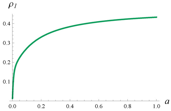
Figure 2.
Correlation of two consecutive transmission times, , versus parameter a.
In what follows, when manipulating a, rather than giving a in the plots, the value of is presented, which is more interesting. Regardless of the value of a, the service rate for these matrices remains unaltered and equal to 100 pkts/s.
The packet interarrival interval distribution is
where b is a parameter. No matter what b is, the expected arrival rate is 100pkts/s. However, the coefficient of variation for the interarrival interval, C, changes with b. In Figure 3, this relationship is shown.
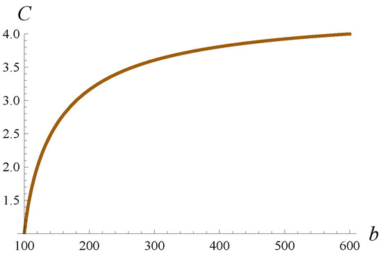
Figure 3.
Coefficient of variation, C, for the time between packets versus parameter b.
When manipulating b, rather than giving b in the plots, the value of C is shown. If not declared otherwise, the buffer volume is . This will be altered in Section 6.1 and Section 6.2, where much larger buffers will be used as well.
In Figure 4, the output traffic intensity in time is depicted for and various values of . In every case, the buffer is initially empty, . In Figure 5, the output traffic intensity is displayed for the same C and various but with an initially full buffer, . In Figure 6, the same curves as in Figure 5 are depicted, but over a much longer time scale.
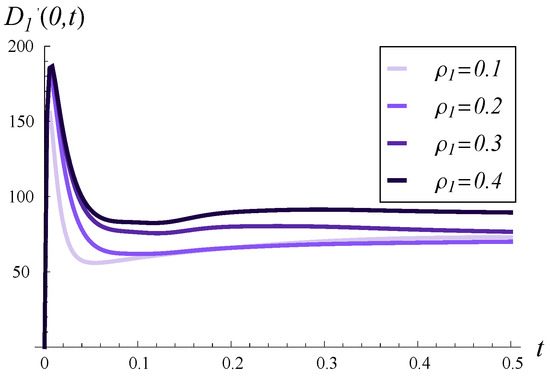
Figure 4.
Output traffic intensity in time for four different values of . and in every case.
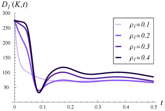
Figure 5.
Output traffic intensity in time for four different values of . and in every case.
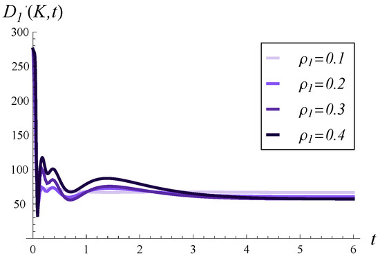
Figure 6.
Output traffic intensity over a long time for four different values of . and in every case.
Therefore, in Figure 4, Figure 5 and Figure 6, we can observe the effect of increasing on the time-dependent output traffic intensity in the case of initially empty buffer versus full buffer (Figure 4 vs. Figure 5), as well as in the short versus long time scale (Figure 5 vs. Figure 6).
In Figure 4, we observe a high peak in the output traffic intensity, approaching 200, shortly after the start. This peak is not related to but is solely caused by the high value of C (this will also be discussed next to Figure 7). The initial intensity in Figure 5 is even higher, being nearly 300. Such high intensity is a reaction to the initially full buffer, meaning the service process can depart several packets from the buffer without waiting for new arrivals.
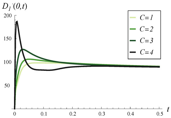
Figure 7.
Output traffic intensity in time for four different values of C. and in every case.
Growing service correlation has at least two noticeable effects in Figure 4, Figure 5 and Figure 6. Firstly, a high may increase the output traffic intensity over a short time scale, as seen in both Figure 4 and Figure 5. This can be attributed to the fact that a high positive correlation induces short periods of higher-than-average service intensity. Over a longer time scale, the effect is reversed, i.e., a higher leads to lower output traffic intensity, as evident in Figure 6. Secondly, high service correlation can cause a complex evolution of the intensity, especially visible in Figure 5 and Figure 6. Specifically, several local minima and maxima may occur over time, and their magnitudes are clearly related to the strength of the correlation—the higher , the more pronounced these extrema become.
Another consequence of high service correlation is the convergence time to a stable throughput, as seen in Figure 6. Namely, the higher is, the more time is required for the throughput to stabilize at the stationary value.
In Figure 7, the output traffic intensity over time is illustrated for and various C values. In each case, the buffer is initially empty, i.e., . In Figure 8, the output traffic intensity is depicted for the same and various C values but with an initially full buffer, i.e., . In Figure 9, the same curves as in Figure 8 are depicted, but over a longer time scale.
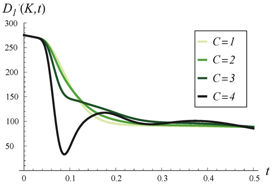
Figure 8.
Output traffic intensity in time for four different values of C. and in every case.
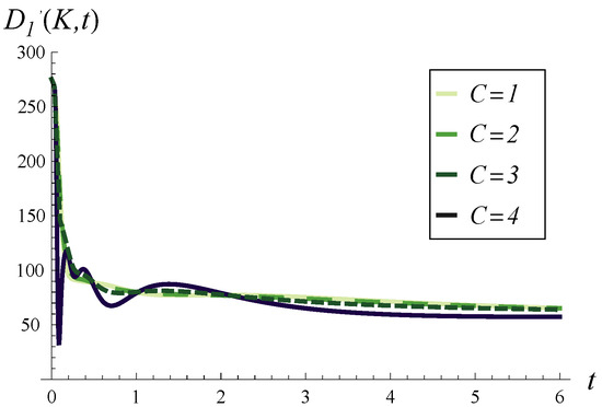
Figure 9.
Output traffic intensity over a long time for four different values of C. and in every case.
Thus, Figure 7, Figure 8 and Figure 9 aim to demonstrate the effect of increasing C on the time-dependent output traffic intensity, comparing the case of an initially empty buffer versus an initially full buffer (Figure 7 vs. Figure 8) and short-term versus long-term behavior (Figure 8 vs. Figure 9).
As seen in Figure 7, for the initially empty buffer, a high initial peak in output traffic intensity is caused solely by high values of C. As C decreases, this peak diminishes accordingly. Conversely, the high initial intensity in Figure 8 is due to the strong correlation and the full buffer, meaning several packets from the buffer can be processed quickly without waiting for new arrivals.
In Figure 9, we may examine the convergence to the stable throughput depending on C. As seen, C impacts the variability in output traffic intensity during the initial short time but has a minor effect on the total convergence time. For every C, the convergence time is more or less the same. The difference is that for a small C, the convergence is more regular and monotonic, while for a high C, it is more variable, with local extrema.
In Figure 10 and Figure 11, the loss intensity over time is illustrated for three initial buffer occupancies (0%, 50%, and 100%). In both figures, a small is assumed. However, the figures differ in the correlation: in Figure 10, compared to in Figure 11.
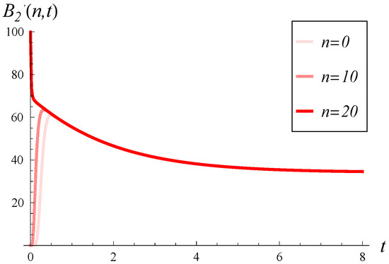
Figure 10.
Loss intensity in time for three different initial buffer occupancies, n. and in every case.
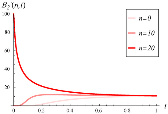
Figure 11.
Loss intensity in time for three different initial buffer occupancies, n. and in every case.
As we observe, has a tremendous impact on the loss intensity, even when C is small. For a high in Figure 10, very high loss intensities are observed, often exceeding 50, even when the buffer is initially empty. Conversely, for a small in Figure 11, high intensities are observed only for a short time and only for an initially full buffer.
Now, in Figure 12, the dependence of throughput, T, on both C and is depicted. Moreover, in Figure 13 and Figure 14, several vertical slices of Figure 12 are shown. Specifically, Figure 13 displays four slices at different values, while Figure 14 presents four slices at different C values.
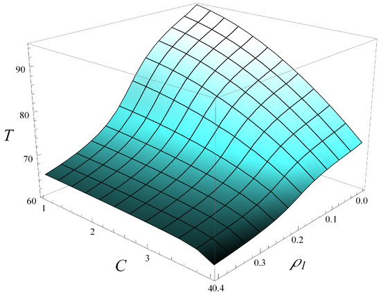
Figure 12.
Stationary throughput versus C and .
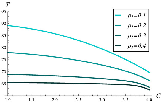
Figure 13.
Stationary throughput versus C for four different values of .
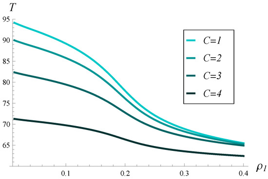
Figure 14.
Stationary throughput versus for four different values of C.
As seen in Figure 12, Figure 13 and Figure 14, increasing C and has a similar impact on the degradation of throughput, at least when C varies up to 4 and varies up to 0.4. The impact of is slightly stronger than that of C, meaning the throughput decreases faster with increasing than with increasing C.
Finally, in Figure 15, the dependence of the stationary loss probability, P, on both C and is depicted. As seen, increasing C and increases the loss probability, while the impact of is slightly stronger than that of C, meaning P increases faster with than with C.
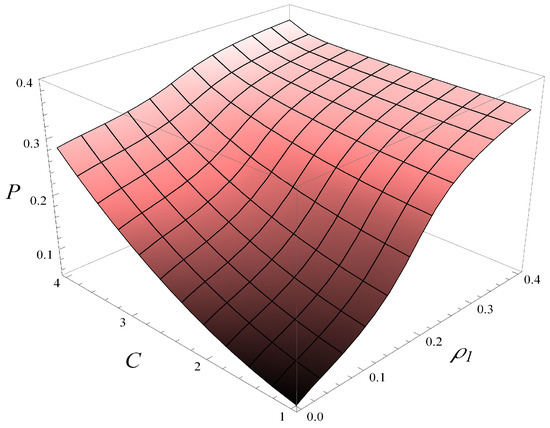
Figure 15.
Stationary loss probability versus C and .
Note that in the stationary case, throughput and loss probability are complementary; if one of them is high, the other must be low, and vice versa. However, this is not true when considering time-dependent output traffic intensity and loss intensity. Specifically, at certain points in time, both output traffic intensity and loss intensity can be high. This can occur, for instance, after a buffer overflow event. The loss intensity remains high for some time before vacant space in the buffer opens up, while the output traffic intensity can also be high because the service process can utilize packets from the buffer without waiting for new arrivals.
6.1. Dependence on Buffer Size
So far, only a buffer of size 20 packets has been used. Now, we will increase the buffer size and check how it influences the throughput of the buffer.
In Figure 16, the dependence of the stationary throughput on the buffer size is depicted. Five different correlations of transmission times are used, ranging from no correlation, , up to . As was easy to predict, in every case, the throughput grows monotonically with the buffer capacity. It is more interesting to see how the correlation strength influences the throughput as the buffer capacity grows. For no correlation or a weak correlation , an almost maximal throughput of 100 pkts/s is achieved for a buffer sizes of about 400 packets. For a mild correlation of , it equals 96.71 pkts/s when . For and , however, the throughput is far from the maximum, even for . In fact, if , the throughput is only 83.38 pkts/s and grows very slowly with the buffer capacity.
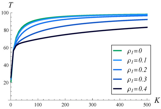
Figure 16.
Stationary throughput T versus buffer size K for five different values of . .
All of these observations illustrate again the strong effect that the correlation of transmission times has on throughput.
6.2. Dependence on Traffic Intensity
In all the previous examples, the arrival rate was equal to the service rate, resulting in a traffic intensity of 1 in every scenario.
Now, we will decrease the traffic intensity and check how this influences the throughput of the buffer. To achieve that, the arrival rate will be kept unaltered, i.e., 100 pkts/s, as follows from (73), but the service rate will be increased to , where is a parameter. To accomplish this, it suffices to use matrices and rather than the original and from (72) and (71), respectively. The resulting traffic intensity is then .
In Figure 17, the dependence of the stationary throughput on the buffer size is shown. Four different values of traffic intensity are used, ranging from to 1. In every case, a mild correlation of is applied. As seen, when the traffic intensity is 0.6 or less, a buffer of size 150 suffices to achieve the maximal throughput. When the traffic intensity is 0.8, a buffer for 300 packets is needed. Finally, when the traffic intensity is 1, the buffer capacity must be greater than 500 to maximize the throughput.
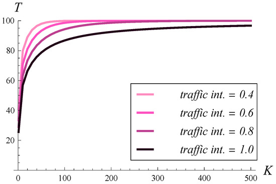
Figure 17.
Stationary throughput T versus buffer size K, for four different values of traffic intensity. and .
6.3. Verification via Simulations
The theoretical throughput of the buffer was also verified through simulations. Specifically, the exact model defined in Section 3 was implemented in a discrete-event simulator environment, OMNeT++ [3], and parameterized according to (71)–(73). Then, 16 simulations were performed with different combinations of C and . In each simulation run, packets passing through the system were simulated, and the experimental throughput was recorded.
The numbers are listed in Table 1. Each entry consists of both the theoretical and simulated throughput. As seen, for every combination of C and , the theoretical throughput aligns well with the experimental value.

Table 1.
Theoretical versus simulated throughput for various combinations of and C (. , traffic intensity = 1.
7. Conclusions
We studied the throughput and losses of a buffer whose service times are stochastically dependent. We derived formulae for the count of packets processed and lost in an arbitrary period, the temporary output traffic intensity, the temporary intensity of packet losses, buffer throughput, and loss probability. Analytical findings were accompanied by numeric calculations that demonstrated the influence of the correlation coefficient of consecutive service times, the standard deviation of the interval between packets, and initial buffer occupancy on the throughput and related characteristics. Theoretical results were confirmed in discrete-event simulations.
Future work can focus on two directions. Firstly, other important characteristics of the same model can be investigated. For instance, to the best of the author’s knowledge, the time-dependent workload of the system has not been explored so far. Secondly, the model itself can be further modified and expanded to include, e.g., a group arrival process, a group service process, etc., and then studied with respect to time-dependent characteristics.
Funding
This research received no external funding.
Data Availability Statement
Data is contained within the article.
Conflicts of Interest
The author declares no conflict of interest.
References
- Lel, W.; Taqqu, M.; Willinger, W.; Wilson, D. On the self-similar nature of ethernet traffic (extended version). IEEE/ACM Trans. Netw. 1994, 2, 1–15. [Google Scholar]
- Emmert, B.; Binzenhöfer, A.; Schlosser, D.; Weiß, M. Source traffic characterization for thin client based office applications. Lect. Notes Comput. Sci. 2007, 4606, 86–94. [Google Scholar]
- Available online: https://omnetpp.org/ (accessed on 4 March 2025).
- Morris, R. TCP behavior with many flows. In Proceedings of the International Conference on Network Protocols, Atlanta, GA, USA, 28–31 October 1997; pp. 205–211. [Google Scholar]
- Sun, J.; Zukerman, M.; Ko, K.T.; Chen, G.; Chan, S. Effect of large buffers on TCP queueing behavior. Proc. IEEE INFOCOM 2004, 2, 751–761. [Google Scholar]
- Appenzeller, G.; Keslassy, I.; McKeown, N. Sizing router buffers. ACM SIGCOMM Comput. Commun. Rev. 2004, 34, 281–292. [Google Scholar] [CrossRef]
- Timmer, M.; de Boer, P.T.; Pras, A. How to identify the speed limiting factor of a tcp flow. In Proceedings of the IEEE/IFIP Workshop on End-to-End Monitoring Techniques and Services, Vancouver, BC, Canada, 3 April 2006; pp. 17–24. [Google Scholar]
- Araujo, J.T.; Landa, R.; Clegg, R.G.; Pavlou, G.; Fukuda, K. On rate limitation mechanisms for TCP throughput: A longitudinal analysis. Comput. Netw. 2017, 113, 159–175. [Google Scholar] [CrossRef]
- McKeown, N.; Appenzeller, G.; Keslassy, I. Sizing router buffers (redux). ACM SIGCOMM Comput. Commun. Rev. 2019, 49, 69–74. [Google Scholar] [CrossRef]
- Salvador, P.; Pacheco, A.; Valadas, R. Modeling IP traffic: Joint characterization of packet arrivals and packet sizes using BMAPs. Comput. Netw. 2004, 44, 335–352. [Google Scholar] [CrossRef]
- Mills, K.L.; Schwartz, E.J.; Yuan, J. How to model a TCP/IP network using only 20 parameters. In Proceedings of the Winter Simulation Conference, Baltimore, MD, USA, 5–8 December 2010; pp. 849–860. [Google Scholar]
- Kolesnikov, A. Load Modelling and Generation in IP-Based Networks; Springer: Berlin/Heidelberg, Germany, 2017. [Google Scholar]
- Chen, G.; Xia, L.; Jiang, Z.; Peng, X.; Chen, L.; Bai, B. A two-step fitting approach of Batch Markovian arrival processes for teletraffic data. In Proceedings of the Performance Evaluation Methodologies and Tools: 14th EAI International Conference, VALUETOOLS 2021, Virtual Event, 30–31 October 2021; Springer: Berlin/Heidelberg, Germany, 2021; pp. 22–35. [Google Scholar]
- Bocharov, P.P. Stationary distribution of a finite queue with recurrent flow and Markovian service. Autom. Remote Control 1996, 9, 66–78. (In Russian) [Google Scholar]
- Alfa, A.S.; Xue, J.; Ye, Q. Perturbation theory for the asymptotic decay rates in the queues with Markovian arrival process and/or Markovian service process. Queueing Syst. 2000, 36, 287–301. [Google Scholar] [CrossRef]
- Bocharov, P.P.; D’Apice, C.; Pechinkin, A.V.; Salerno, S. The stationary characteristics of the G/MSP/1/r queueing system. Autom. Remote Control 2003, 64, 288–301. [Google Scholar] [CrossRef]
- Albores-Velasco, F.J.; Tajonar-Sanabria, F.S. Analysis of the GI/MSP/c/r queueing system. Inf. Processes 2004, 4, 46–57. [Google Scholar]
- Gupta, U.C.; Banik, A.D. Complete analysis of finite and infinite buffer GI/MSP/1 queue—A computational approach. Oper. Res. Lett. 2007, 35, 273–280. [Google Scholar] [CrossRef]
- Banik, A.D.; Gupta, U.C. Analyzing the finite buffer batch arrival queue under Markovian service process: GIX/MSP/1/N. Top 2007, 15, 146–160. [Google Scholar] [CrossRef]
- Banik, A.D. Analyzing state-dependent arrival in GI/BMSP/1/∞ queues. Math. Comput. Model. 2011, 53, 1229–1246. [Google Scholar] [CrossRef]
- Chaudhry, M.L.; Samanta, S.K.; Pacheco, A. Analytically explicit results for the GI/C-MSP/1/∞ queueing system using roots. Probab. Eng. Inf. Sci. 2012, 26, 221–244. [Google Scholar] [CrossRef]
- Samanta, S.K. Sojourn-time distribution of the GI/MSP/1 queueing system. Opsearch 2015, 52, 756–770. [Google Scholar] [CrossRef]
- Chaudhry, M.L.; Banik, A.D.; Pacheco, A. A simple analysis of the batch arrival queue with infinite-buffer and Markovian service process using roots method: GIX/C-MSP/1/∞. Ann. Oper. Res. 2017, 252, 135–173. [Google Scholar] [CrossRef]
- Banik, A.D.; Chaudhry, M.L.; Kim, J.J. A Note on the Waiting-Time Distribution in an Infinite-Buffer GI[X]/C-MSP/1 Queueing System. J. Probab. Stat. 2018, 2018, 7462439. [Google Scholar] [CrossRef]
- Banik, A.D.; Ghosh, S.; Chaudhry, M.L. On the consecutive customer loss probabilities in a finite-buffer renewal batch input queue with different batch acceptance/rejection strategies under non-renewal service. In Soft Computing for Problem Solving: SocProS 2017; Springer: Singapore, 2019; Volume 1, pp. 45–62. [Google Scholar]
- Banik, A.D.; Ghosh, S.; Chaudhry, M.L. On the optimal control of loss probability and profit in a GI/C-BMSP/1/N queueing system. Opsearch 2020, 57, 144–162. [Google Scholar] [CrossRef]
- Samanta, S.K.; Bank, B. Modelling and Analysis of GI/BMSP/1 Queueing System. Bull. Malays. Math. Sci. Soc. 2021, 44, 3777–3807. [Google Scholar] [CrossRef]
- Chydzinski, A. Transient GI/MSP/1/N Queue. Entropy 2024, 26, 807. [Google Scholar] [CrossRef] [PubMed]
- Chydzinski, A. Time to reach buffer capacity in a BMAP queue. Stoch. Model. 2007, 23, 195–209. [Google Scholar] [CrossRef]
- Dudin, A.N.; Klimenok, V.I.; Vishnevsky, V.M. The Theory of Queuing Systems with Correlated Flows; Springer: Cham, Switzerland, 2020. [Google Scholar]
- Zakian, V. Numerical inversion of Laplace transform. Electron. Lett. 1969, 5, 120–121. [Google Scholar] [CrossRef]


Disclaimer/Publisher’s Note: The statements, opinions and data contained in all publications are solely those of the individual author(s) and contributor(s) and not of MDPI and/or the editor(s). MDPI and/or the editor(s) disclaim responsibility for any injury to people or property resulting from any ideas, methods, instructions or products referred to in the content. |
© 2025 by the author. Published by MDPI on behalf of the International Institute of Knowledge Innovation and Invention. Licensee MDPI, Basel, Switzerland. This article is an open access article distributed under the terms and conditions of the Creative Commons Attribution (CC BY) license (https://creativecommons.org/licenses/by/4.0/).