Abstract
The healthcare industry has recently faced the issues of enhancing patient care, streamlining healthcare operations, and offering high-quality services at reasonable costs. These crucial issues include general healthcare administration, resource allocation, staffing, patient care priorities, and effective scheduling. Therefore, efficient staff scheduling, resource allocation, and patient assignments are required to address these challenges. To address these challenges, in this paper, we developed a mixed-integer linear programming (MILP) model employing the Gurobi optimization solver. The model includes staff assignments, patient assignments, resource allocations, and overtime hours to minimize healthcare expenditures and enhance patient care. We experimented with the robustness and flexibility of our model by implementing two distinct scenarios, each resulting in two unique optimal solutions. The first experimental procedure yielded an optimal solution with an objective value of 844.0, with an exact match between the best-bound score and the objective value, indicating a 0.0% solution gap. Similarly, the second one produced an optimal solution with an objective value of 539.0. The perfect match between this scenario’s best-bound score and objective value resulted in a 0.0% solution gap, further affirming the model’s reliability. The best-bound scores indicated no significant differences in these two procedures, demonstrating that the solutions were ideal within the allowed tolerances.
1. Introduction
Healthcare organizations aim to efficiently manage limited resources to provide high-quality, cost-effective care while maximizing patient satisfaction. Key challenges include minimizing expenditures, optimizing resource allocation, and strategically scheduling staff, patients, and resources. Effective scheduling through careful assignment of personnel and resources is vital for healthcare systems to maximize operational efficiency and the quality of patient care [1,2]. In hospitals, the managerial component of patient care continues to take on increasing significance. Moreover, healthcare providers devote considerable effort to managing these resources effectively to ensure high-quality patient care and maximum operational efficiency. Increased staff productivity and optimal resource utilization resulting from effective scheduling can improve patient outcomes [3]. Patient care improvement pertains to an increase in the efficiency of staff and resource allocation, leading to enhanced patient satisfaction and health outcomes. This could be measured using a combination of methods, including patient satisfaction surveys, health outcomes, process measures, patient safety indicators, and efficiency measures, depending on the specific goals of the healthcare organization. Furthermore, globally, the increased pressure from factors such as the immense and escalating cost of healthcare, standard expectations from patients, and aging populations is challenging the healthcare industry, and the need to devise a panacea for these recurring issues is vital [4]. The importance of having the appropriate staff in the ideal location at the right time was highlighted during the COVID-19 pandemic because of the unpredictably high volume and fluctuating needs for care delivery. Aging staff and patients, a nursing shortage, and an increase in the complexity of care across all settings exacerbated the operational constraints of the pandemic [5]. Healthcare management relies on staff schedules. This involves overseeing patient appointments, predicting patient service demands, monitoring the availability of doctors and nurses, and implementing automated resource allocation. Urgent care medical centers and emergency rooms might require assistance in projecting patient influx against staff availability. Despite the prevalence of schedule optimization in various industries, many organizations continue to adopt this practice. Efficient scheduling not only reduces patient wait times but also optimizes resource utilization [6].
1.1. Challenges Confronting the Current Healthcare System
Effectively allocating limited resources is vital for optimizing patient care and achieving satisfactory outcomes. In recent years, the healthcare system has faced various challenges associated with limited resources regarding staff shortage, staff and patient time slots and scheduling, and equipment. However, maintaining an optimal healthcare system for these challenges is complex, making it an operation research problem [7]. Hence, hospitals must proactively maximize their limited resources and reduce patient wait times to address these challenges. Moreover, this sector must aim to strategize decisions to minimize total functional costs and maximize patient satisfaction. Therefore, the research addresses these challenges by developing an optimization model.
1.2. Research Context and Significance
We developed a mixed-integer linear programming (MILP) model, which offers a quantitative and systematic approach to healthcare resource allocation, staff, and patient scheduling. The model uses mathematical optimization techniques that consider the necessary variables related to healthcare management to minimize costs and improve patient care. Moreover, this approach ensures that the resources are utilized most efficiently by maximizing their potential values.
For example, our research proposes a novel model that can significantly support demand and volume forecasting while considering staff availability for urgent care medical facilities and emergency rooms. Employing this model in these healthcare settings can assist these hospitals in optimizing staff scheduling and resource allocation to meet variable patient demands. Moreover, optimizing resource allocation, staff scheduling, and patient assignment is required to address the above issues. Our MILP technique employs mathematical optimization to minimize expenses while enhancing patient care. Our approach ensures that healthcare management factors and constraints are considered to maximize the utilization of resources.
The model focuses on new elements by employing a tailored mathematical optimization environment incorporating specific ranges and variables relevant to healthcare scheduling. While generic models allocate resources based solely on demand and capacity, we tailor our approach according to the specific dynamics of each hospital or clinic, ensuring optimal care for all patients. We addressed the optimization problem with increased flexibility by employing Python programming. In addition, the new elements involved in the model are resource allocation and staff working hours, which have yet to be included in other research in combination with all other elements.
The remainder of this paper addresses the related work in healthcare scheduling (staff, patients, and resources), the application of mathematical models to healthcare, the proposed model’s mathematical formulation, the model algorithm, the methodology, results, and discussions, the conclusion, implications for healthcare management and staffing procedures, and directions for future research.
2. Related Work
This section provides an overview of the literature concerning the application of mathematical modeling in the healthcare system. Numerous researchers have studied this field intensely, contributing to a growing body of related work. The following literature review presents the key findings and advancements in mathematical models applied to healthcare.
Over the years, mathematical models such as linear programming (LP), MILP, dynamic programming (DP), integer programming (IP), stochastic programming, network optimization, queuing theory, game theory [8,9,10,11,12,13,14,15,16], system dynamics models, and agent-based models [17,18] have been employed to solve complex healthcare optimization problems.
Healthcare Scheduling and Resource Optimization
Efficient healthcare scheduling and resource management is critical for operational efficiency. Literature in this domain applies mathematical optimization to crucial areas like staff and patient scheduling, admission planning, and resource allocation. For staff scheduling, the research aims to optimize shift scheduling and nurse routing models using techniques such as mixed-integer programming and genetic algorithms [19,20,21]. Approaches consider nurse availability, hospital policies, and workload balancing. Optimization in patient admission and appointment systems reduces wait times through simulation, algorithms, and queuing models [22,23,24]. Methods incorporate patient priorities and time slot preferences [25,26]. Additional studies apply optimization techniques such as stochastic programming, network modeling, and machine learning for resource allocation, bed management, and operating room scheduling [27,28,29]. The healthcare scheduling literature leverages operations research to optimize staff planning, patient scheduling, and resource allocation. Mathematical modeling provides quantitative approaches for maximizing utilization, service quality, and productivity.
The existing literature centers around specific aspects of healthcare management and scheduling, while the proposed model uniquely targets healthcare scheduling. It emphasizes the intricate balance between resource allocation, patient satisfaction, and operational efficiency. Unlike previous work, the model thoroughly examines healthcare resource allocation, encompassing staff, patients, and resources over specified periods. This approach enables more precise and context-sensitive optimization aligned with healthcare organizations’ demands. Despite the focused nature of prior models, our approach offers a comprehensive and integrated approach to optimize healthcare operations. It employs mathematical procedures with simulated data to handle a wide array of healthcare operations based on staff scheduling, patient assignment, and resource allocation using linear and integer programming for a holistic optimization approach.
3. Model Mathematical Formulation
This section explores a complex mathematical formulation model for scheduling challenges in healthcare settings. The suggested approach intends to maximize the allocation of resources, the assignment of staff members to time slots, the assignment of patients to time slots, and the management of overtime and penalties. The objective is to minimize the total cost of these assignments and allocations while maintaining the schedule’s viability and efficiency under various restrictions. The binary decision variables in this model represent different assignments and allocations. This model exemplifies an integer programming problem, a standard optimization problem category in operations research.
3.1. Problem Description
We optimize healthcare delivery by assigning staff, scheduling patients, and allocating resources. This research aims to minimize healthcare delivery and operational costs and to improve efficiency. We then further explain staff availability, patient demand, resource availability, and budgets in healthcare settings based on decision constraints.
3.2. Variables and Parameters
Let us introduce the following variables and parameters:
- : Binary decision variable indicating whether staff member i is assigned to time slot t.
- : Binary decision variable indicating whether patient p is assigned to time slot t.
- : Binary decision variable indicating whether resource r is allocated at time slot t.
- : Binary decision variable indicating whether staff member i works overtime.
- : Binary decision variable indicating whether staff member i serves patient p.
- : The weight associated with assigning staff member i to time slot t. This could represent the cost or importance of this assignment.
- : The interaction weight between staff members i and j at time slot t when both are assigned to work. This could reflect the benefit or cost of having these two staff members work together.
- : The cost associated with assigning patient p to time slot t. This could represent the cost of providing service to this patient at this time.
- : The cost associated with allocating resource r at time slot t. This could represent the cost of using this resource at this time.
- : The penalty associated with patient p not receiving service during time slot t. This could reflect the negative impact of not serving this patient at this time.
- : The overtime weight for staff member i when they work overtime. This could represent the extra cost or penalty for having this staff member work beyond their regular hours.
- : The weight associated with patient p not receiving service when staff member i serves them. This could reflect the negative impact of not serving this patient when this staff member is working.
- : The skill level of staff member i required for serving patients during time slot t. This could represent the ability of this staff member to provide service.
- : The demand for staff at time slot t. This could represent the number of staff members needed at this time.
- : The maximum working hours for staff member i. This could represent the maximum number of time slots this staff member can be assigned to.
- : The minimum skill level of staff member i required for serving patient p in task k during time slot t. This could represent the minimum ability needed to provide this service.
- B: The budget constraint. This could represent the maximum total cost of staff assignments and resource allocations.
- : The maximum allowed difference in working hours between staff members i and j. This could represent the maximum disparity in workload between these two staff members.
3.3. Objective Function
Our objective is to minimize the total cost of staff assignments, patient scheduling, and resource allocation while maximizing the efficiency of healthcare delivery. The following objective function represents this:
Objective Function Terms
- 1
- : This term represents the weight associated with assigning staff member i to time slot t.
- 2
- : This term represents the interaction weight between staff members i and j at time slot t when both are assigned to work.
- 3
- : This term represents the cost associated with assigning patient p to time slot t.
- 4
- : This term represents the cost associated with allocating resource r at time slot t.
- 5
- : This term represents the penalty associated with patient p not receiving service during time slot t.
- 6
- : This term represents the overtime weight for staff member i when they work overtime.
- 7
- : This term represents the weight associated with patient p not receiving service when staff member i serves them.
- 8
- : This term represents the skill level of staff member i required for serving patients during time slot t.
3.4. Constraints
The decisions are subject to the following constraints:
- 1
- Staff Availability: The total number of staff members assigned to each time slot must equal the demand for staff at that time.
- 2
- Maximum Working Hours: The total number of time slots each staff member can be assigned to is limited by their maximum working hours.
- 3
- Patient Scheduling: Each patient is assigned to exactly one time slot.
- 4
- Resource Allocation: Each resource is allocated to exactly one time slot.
- 5
- Skill Level: The skill level of each staff member assigned to serve a patient in a task during a time slot must be at least equal to the minimum skill level required for that task.
- 6
- Overtime: If a staff member works overtime, the sum of their assigned time slots must exceed their maximum working hours.
- 7
- Budget Constraint: The total cost of staff assignments and resource allocations must not exceed the budget constraint.
- 8
- Workload Balance: The difference in working hours between any two staff members must be within the maximum allowed difference.
The decision variables , , , , and are all binary, i.e., they take values in .
3.5. Model Algorithm
Algorithm 1 describes the healthcare scheduling model optimization process. First, in the algorithm, libraries and input data parameters are imported. Afterward, the model is generated using the input data parameters, including the number of staff members (N), time slots (T), patients (P), resources (R), tasks (K), staff work hours (W), interaction between staff members (I), patient care time (C), resource demand (D), patient quality of care (Q), overtime hours (O), patient urgency (U), staff skill level (S), task matching (M), staff hours (H), total demand (Dt), overtime budget (B), and staff familiarity (F). Decision variables, such as x, y, z, o, and v, reflect scheduling constraint characteristics. Moreover, the objective function minimizes . Staff hours, availability, patient slot allocation, resource slot allocation, overtime budget, patient-staff relationship, and task-staff interaction are constrained. Optimizing the model seeks the ideal solution. If an optimal solution is discovered, the algorithm outputs the respective values for the staff, patients, resources, and overtime hours.
| Algorithm 1 Healthcare Scheduling Optimization |
|
4. Methodology
This section delves into the technical procedures employed in the research. It elaborates on the nature of the data generated for the model and how the mathematical model optimization environment was created.
4.1. Research Input Data
The model’s ranges and variables were created using Python programming to describe the optimization problem components (Note: In Python programming, indexing starts from 0 rather than 1). For the two procedures, the ranges for staff members, time slots, patients, tasks, and resources represented in the first process are: N (1–21), denoting 20 members of staff (including physicians, nurses, surgeons, pharmacists, medical technologists, etc.); T (1–11), 10 time slots in hours; P (1–31), 30 patients; K (1–16), which represents 15 tasks (including administering medication, conducting patient assessments, assisting in surgeries, monitoring vital signs, providing wound care, conducting diagnostic tests, assisting with patient mobility, offering emotional support, collaborating with healthcare professionals, and educating patients on disease management); and R (1–11), which represents 10 allocated resources (including hospital beds, operating rooms, medical equipment, laboratory facilities, radiology equipment, surgical instruments, medications, ambulances, intensive care unit (ICU) beds, anesthesia machines, patient monitoring systems, wheelchairs, surgical supplies, imaging and diagnostic equipment, and personal protective equipment (PPE)). The ranges for the second process are N (1–31), T (1–6), P (1–21), K (1–11), and R (1–16).
The parameters’ dictionaries were generated using the predefined ranges for the two procedures. In the dictionary, I contained random integer values between 1 and 10 for each combination of staff members i and j and time slot. For every staff member i and time slot t combination, the dictionary W included random integer values between 1 and 10. Moreover, we further generated new dictionaries that represented the model’s components. These dictionaries (C, D, Q, O, U, S, M, H, , and F) capture healthcare scheduling optimization model parameters and relationships. Afterward, these new dictionaries were populated with random integer values (C (1–10), D (1–10), Q (1–10), O (1–10), U (1–10), S (1–5), M (1–5), H (8–12), (2–5), and F (1–3)) in preset ranges to simulate data. The model optimization utilized these input data from the inherent simulation to arrive at the optimal value and further analyze it. Hence, for the model, generating random values within the given ranges created a diverse and representative dataset covering healthcare scheduling constraints.
4.2. Flexibility and Optimization Capabilities of the Proposed Healthcare Scheduling Model
The proposed model allows for parameter variation and distinct outputs based on the optimization goals. Healthcare scheduling may be optimized by changing the model’s parameters, including weights, costs, penalties, skill levels, demand, and constraints. This versatility allows the model to be tailored to specific demands, resource availability, patient requirements, and organizational decisions. Considering many aspects and constraints, the model optimizes staff, patients, resources, and time slots. The model’s flexibility and optimization facilitate healthcare scheduling decision-making and process improvement.
4.3. Use of Simulated Data: Overcoming Challenges in Obtaining Real-World Data
During this research, acquiring real-world data that aligns precisely with the specified parameters was challenging owing to diverse practical limitations. Factors such as accessibility, availability, concerns about privacy, and the dynamic state of healthcare systems hindered the availability of suitable data. Nevertheless, it is crucial to address these challenges to guarantee the consistency of health research and decisions. Consequently, a simulated data procedure was employed to address these difficulties and offer a typical setting for carrying out experiments. Moreover, the simulated data enabled controlled experiments, plausible scenarios, and the generation of varied datasets with specific parameter arrangements. Despite circumstances in which collecting real-world data proves tough or impractical, simulated data enabled dependable and precise analysis.
Data Selection for Real-World Healthcare Simulation
The initial data utilized in the simulation model were carefully selected and simulated to represent or mimic real-world healthcare setting scenarios. The selection was guided by intuition and expert judgment and grounded in the following principles:
- Realistic Assumptions: The chosen values for parameters such as working hours, resource utilization, patient demand, and capacity are aligned with typical healthcare practices, regulations, and operational constraints.
- Expert Consultation: Inputs from healthcare practitioners and administrators play a pivotal role. Moreover, experts have informed the selection of initial values, ensuring that they mirror the complexities and nuances of real-world healthcare delivery.
- Sensitivity Analysis: The model’s responsiveness to variations in the initial values have been tested, confirming that the chosen values provide a robust and representative simulation of real-world scenarios.
4.4. Research Materials and System Configuration
We solved the complex healthcare scheduling operation model using the Gurobi Optimizer [30], version 10.0.1, which is a powerful optimization solver. The optimization program ran on an Intel® Core™ i5-6200U CPU @ 2.30GHz with 2 physical cores and 4 logical processors for efficiency. Table 1 shows the research’s system configuration and model information. Our sophisticated mixed-integer linear programming model has 90,101 rows, 1220 columns, and 1,801,420 nonzeros. Despite its complexity, the solver performed well in two optimization techniques. The initial optimization technique yielded five healthcare resource allocation and staff scheduling strategies. The model found an ideal solution with an objective value of 844.0, measuring resource allocation efficiency and effectiveness. The best-bound score, representing the objective function’s theoretical lower limit, was 844.0, demonstrating the solution’s accuracy. The difference between the best objective value and best-bound score was 0.0%, a key model performance parameter. Since the optimal solution and the lower bound of the objective function were identical, the solution was the best within the tolerance limitations.

Table 1.
System configuration and model information.
Furthermore, we optimized the model again to find more subtle solutions. The best of three plausible solutions has an objective value of 539.0, a substantial increase from the first. As with the initial method, the best-bound score matched the objective value, demonstrating the solver’s accuracy. The best objective value and best-bound score were 0.0% apart, demonstrating that the solution was optimal within tolerance. Moreover, branching, a complicated optimization phase, explored 33 nodes and executed 782 simplex iterations. Cutting plane approaches improved convergence and solution quality. Cover cutbacks, mixed integer rounding (MIR), zero-half cuts, relaxation-induced neighborhood search 235 (RINS), and bilinear quadratic pair (BQP) cuts were among these. These methods improved solver speed and precision, which aided optimization.
The two model procedures demonstrated our approach’s robustness and efficacy. The Gurobi solver’s powerful optimization algorithms can address challenging healthcare problems, including resource allocation, staffing, and patient assignment. These findings suggest that healthcare professionals may boost efficiency and quality.
5. Results and Discussions
As shown in Table 2, objective values of 844.0 and 539.0, achieved during the two optimization procedures, represent the overall quality of the desired solutions for these processes. According to the solution counts, 5 possible solutions were discovered throughout the first optimization procedure, while 3 solution counts were achieved during the second process, indicating that the best solutions had the ideal values for the objective functions. The best objective values obtained were 844.0 and 539.0. The best-bound values 844.0 and 539.0 show no significant differences between the best solutions and the objective function’s theoretical lower bounds. Since there is no more opportunity for improvement, the gap values of 0.0% of the two procedures show that the optimal solutions have been found. These findings imply that the optimization procedures effectively located optimal resolutions that meet all constraints and minimize the goal function.
Table 2.
Optimization results for the two model procedures.
Table 3 describes the terms developed during the optimization procedures in great depth. The results are comprehensively analyzed by highlighting their significance and model implications.
Table 3.
Optimization results for first and second outputs.
Table 4 and the subsequent three tables present solutions that include resource allocations, staff overtime hours, patient assignments, and staff assignments for the two model procedures. For the first procedure, staff members (1 to 20) have been assigned to particular time slots (1 to 10). For the second procedure, staff members (1 to 30) have been assigned to particular time slots (1 to 5) in Table 4, reflecting their availability and duties during those times. This distribution aids in deciding on staff resource scheduling and distribution. Regarding patient scheduling, certain patients—1 to 30 for the first procedure and 1 to 20 for the second procedure—have been given specified time slots in Table 5 to ensure they receive the required care within the allotted times. Effective scheduling and patient management depend on these data. Furthermore, resource allocations (1 to 10) for the first procedure and (1 to 15) for the second procedure outline which resources, such as buildings, equipment, etc., are assigned to particular periods.
Table 4.
Staff members’ time slots for first and second outputs.
Table 5.
Patient assignments for first and second outputs.
Table 6 presents this process. This process allows for managing and coordinating resources well to maximize their use. Lastly, for the two procedures, the staff overtime hours (where 0 means no overtime and values beyond 0 mean overtime) show how many extra hours each staff member is expected to work. Table 7 displays this process. Hospital managers can prevent overburdening workers by monitoring and adjusting task distribution using these data. The overall goal of this complete solution is to maximize scheduling and resource allocation in the current situation. It includes numerous staff, patient, and resource management areas in the healthcare system.
Table 6.
Resource allocations for first and second outputs.
Table 7.
Staff overtime hours for first and second outputs.
5.1. Resource Allocations
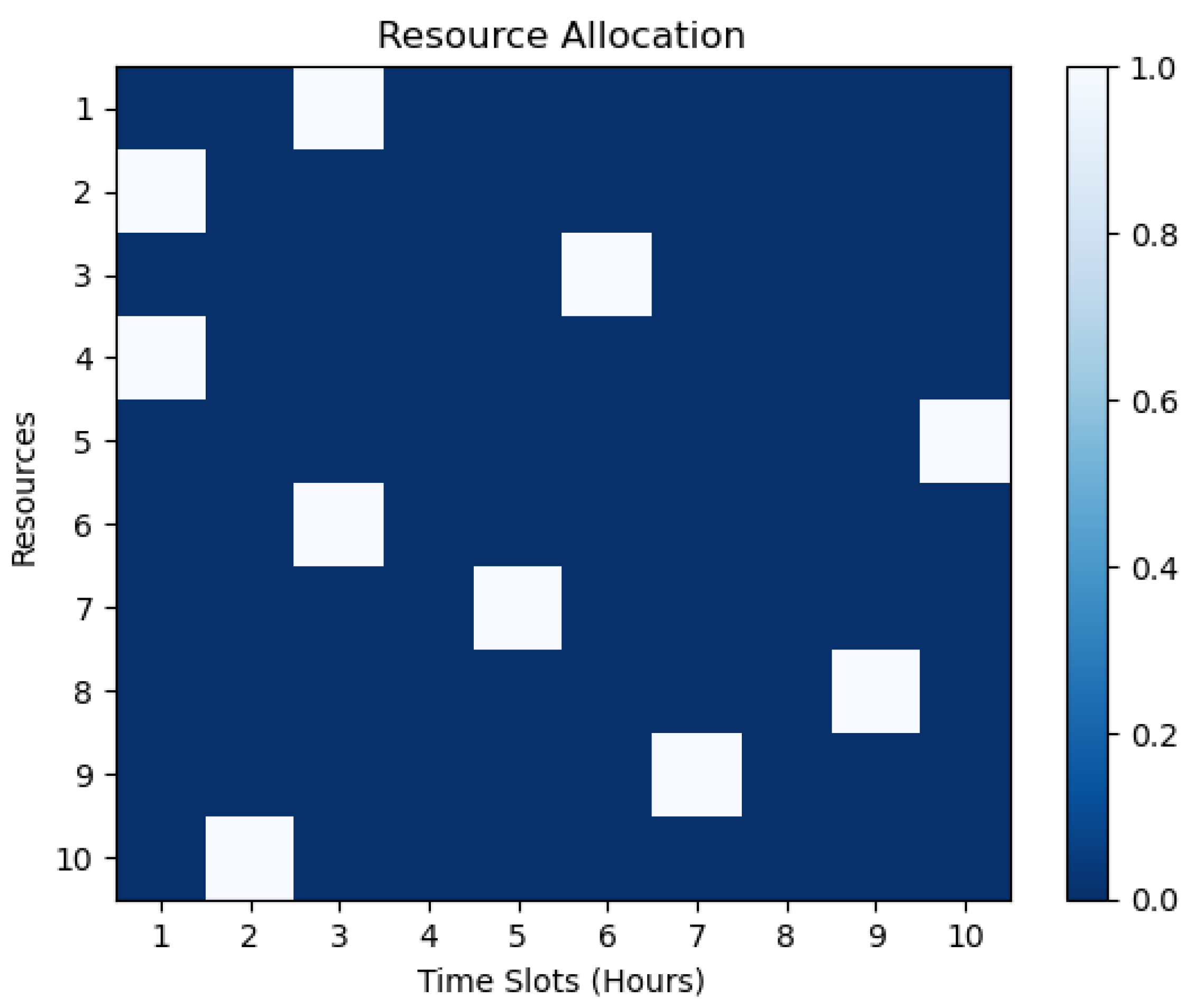
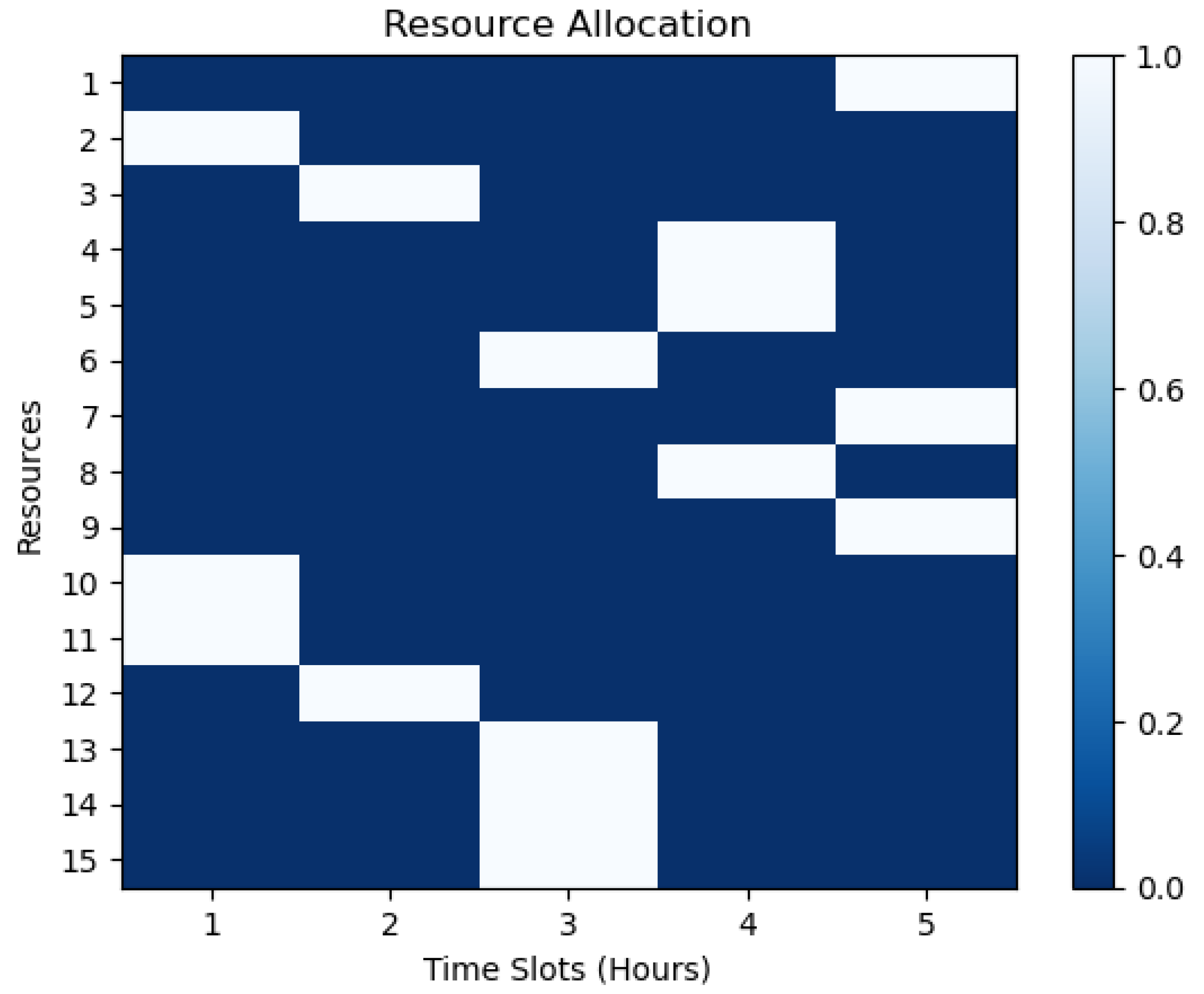
The resource allocation illustrations in Figure 1 and Figure 2 present how healthcare schedule optimization research allocates resources across time slots for the two model procedures. The visualizations show resource consumption and availability during optimization. Each row represents a resource, and each column is a time slot in the heatmap visualization. The darker blue heatmap colors imply more resource allocation at each time slot, whereas the white colors indicate less. The scale on the right side of the graph ranges from 0.0 to 1.0, with 1.0 representing the highest allocation of resources. This scale indicates the percentage of resources allocated at each time slot. For instance, if the scale shows 0.6 at a particular time slot, this means that 60% of the resources are allocated at that time slot. These graphs can be used to analyze hospital resource allocation efficiency and effectiveness by highlighting peak and off-peak resource utilization, gaps and overlaps in resource distribution, and possible areas for improvement or optimization. For example, Figure 1 shows that more resources are allocated in the first hour than in the second. Also, Figure 2 demonstrates that the first two hours had more resources than the next three. This could imply a higher demand for resources in the morning than in the afternoon or an over-allocation of resources in the early hours that should be reassigned to the rest of the hours.
where
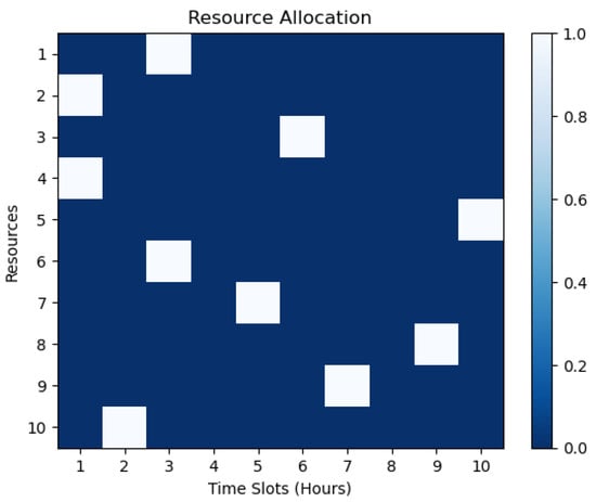
Figure 1.
Resource allocation heatmap for the first model procedure.
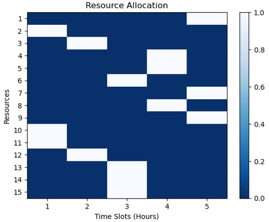
Figure 2.
Resource allocation heatmap for the second model procedure.
- T is the set of time slots;
- R is the set of resources;
- r is a resource from R;
- t is a time slot from T;
- denotes the allocation of resource r at time slot t.
5.2. Patient Distribution
The patient distribution formula is represented as follows:
In this formula, patient_distribution is an array that stores the patient distribution values for each time slot. The variable t represents the time slot index from the set T, and p represents the patient index from the set P. The term represents the value of the variable y for patient p and time slot t.
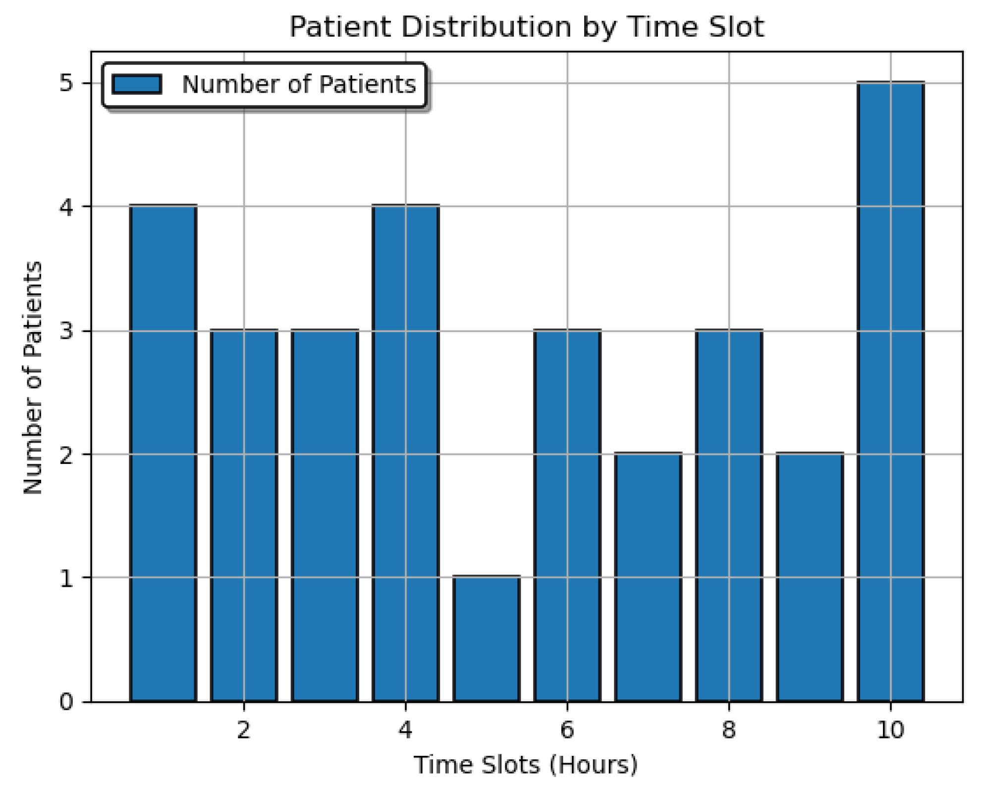
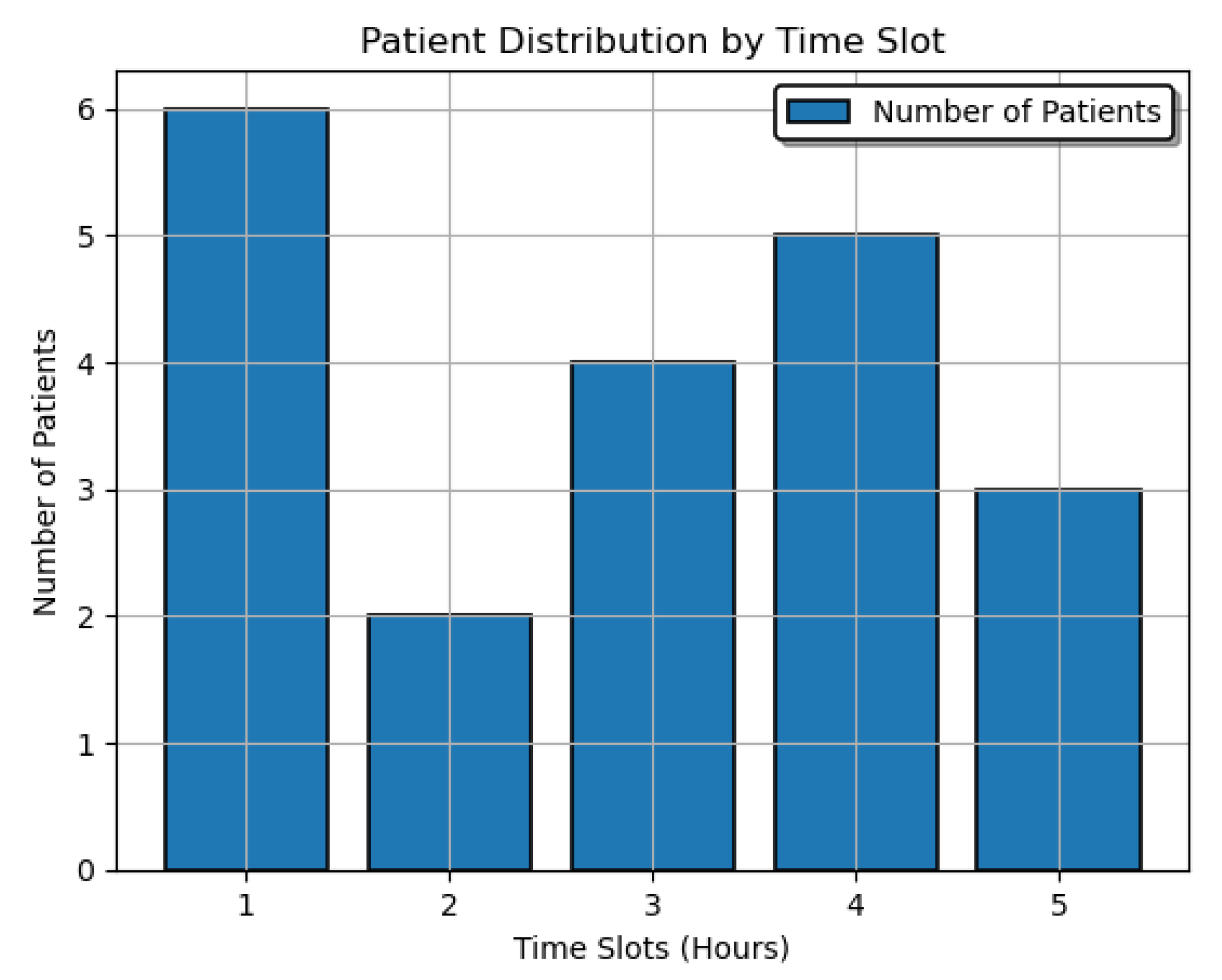
Patient distribution throughout the model’s slated time slots can be observed in Figure 3 and Figure 4. The bar charts for these two procedures illustrate the distribution of patients by time slot in a hospital setting. Figure 3 shows that the hospital is busiest at the 10 h time slot with 5 patients and least busy at the 3 h period, while Figure 4 shows that the hospital is at its busiest at the first hour and least at the second hour. The visualizations can assist healthcare personnel in making decisions based on patient load changes from these scenarios by analyzing patterns and trends in patient distribution.
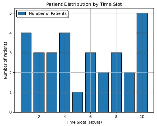
Figure 3.
Patient distribution over time slots for the first model procedure.

Figure 4.
Patient distribution over time slots for the second model procedure.
5.3. Staff Assignment
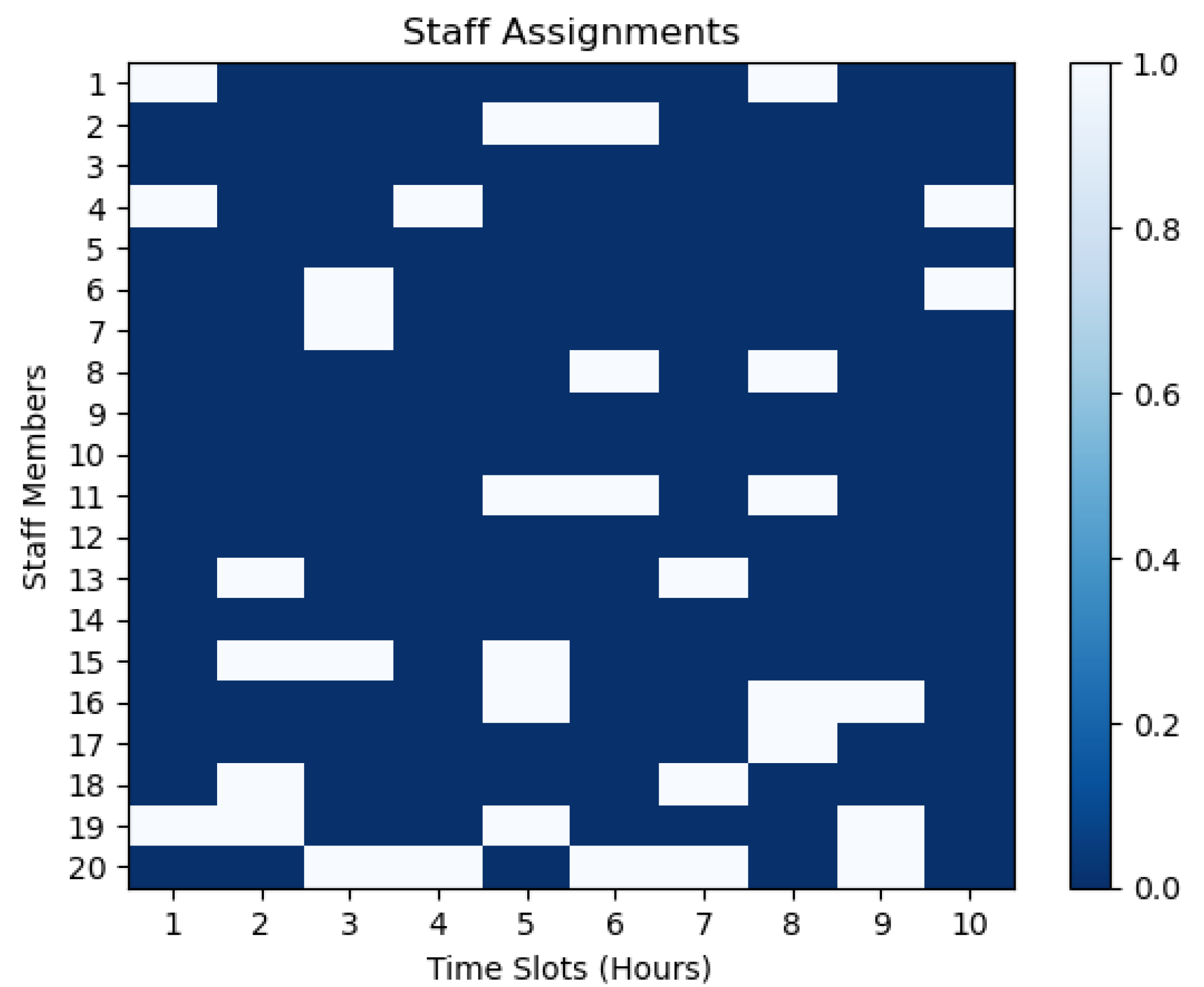
Let be a binary matrix, where i represents the index of staff members, and j represents the index of time slots. if the staff member is assigned to the time slot , and 0 otherwise.
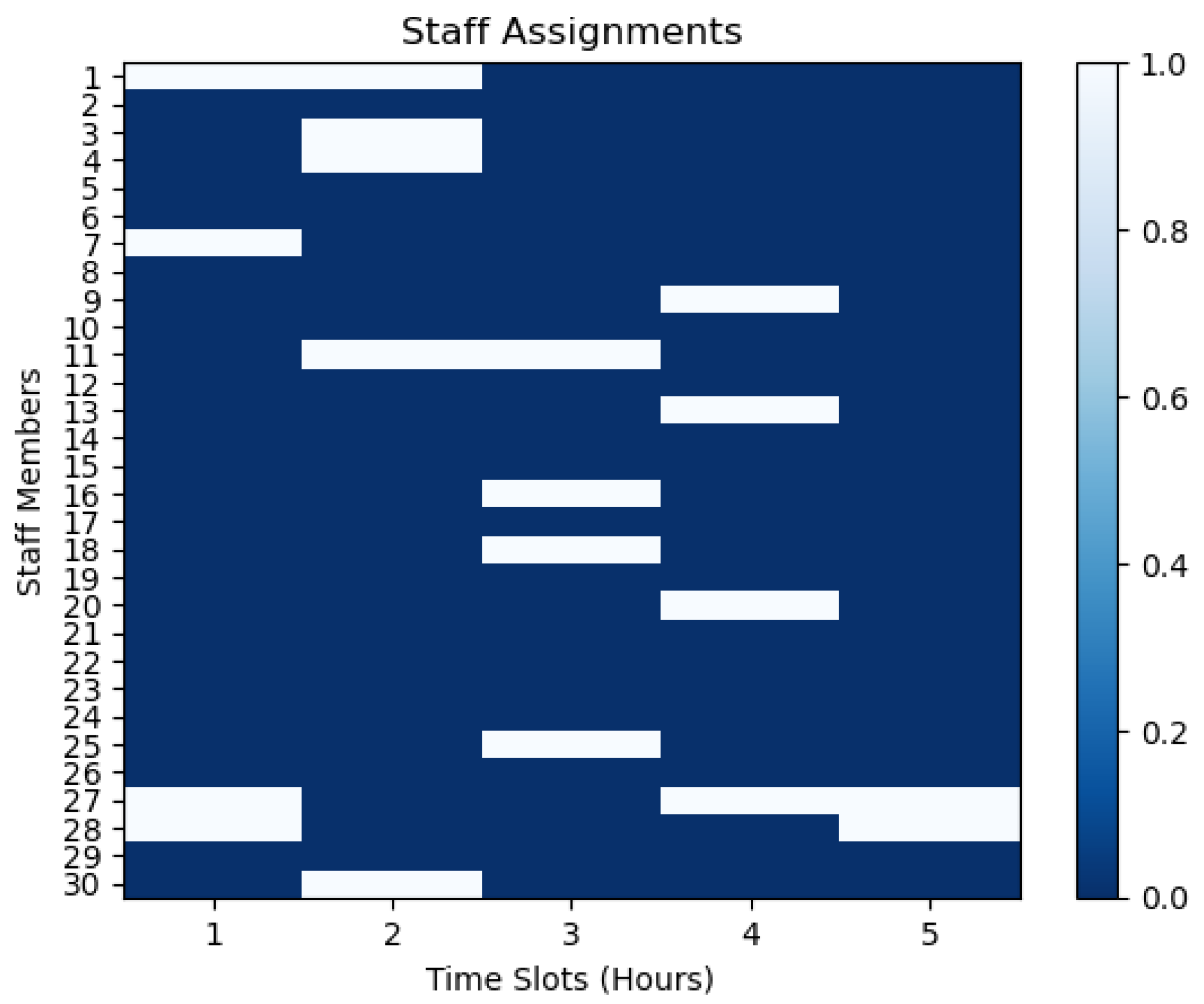
Figure 5 and Figure 6 show the visualizations of the staff members across the slated time slots for the two scenarios in a hospital setting. The heatmaps with right-hand scales in the figures illustrate matrices with staff members on rows and time slots on columns. The darker blue cells indicate the assignment of staff members to specific time slots. The scale on the heatmap’s right side, ranging from 0.0 to 1.0, with 1.0 being the highest, indicates the percentage of staff members assigned at each time slot. For example, if the scale shows 0.4 at a specific time slot, this means that 40% of the staff members are assigned at that time slot. These visualizations aid in optimizing staff assignment and scheduling by providing better decision-making in healthcare management. In the two heatmaps, the staff assignments vary depending on the time slots and the demand for services. In Figure 5, the peak hours are between the 4 h and the 10 h periods, and the lowest for staff assignments are the 5 h and 8 h periods. Also, in Figure 6, the peak hour is the 5 h period, and the lowest for staff assignments is the 2 h period.
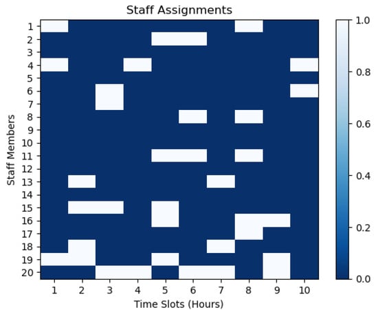
Figure 5.
Staff assignment over time slots for the first model procedure.
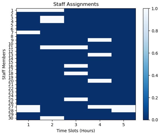
Figure 6.
Staff assignment over time slots for the second model procedure.
5.4. Patient Assignment
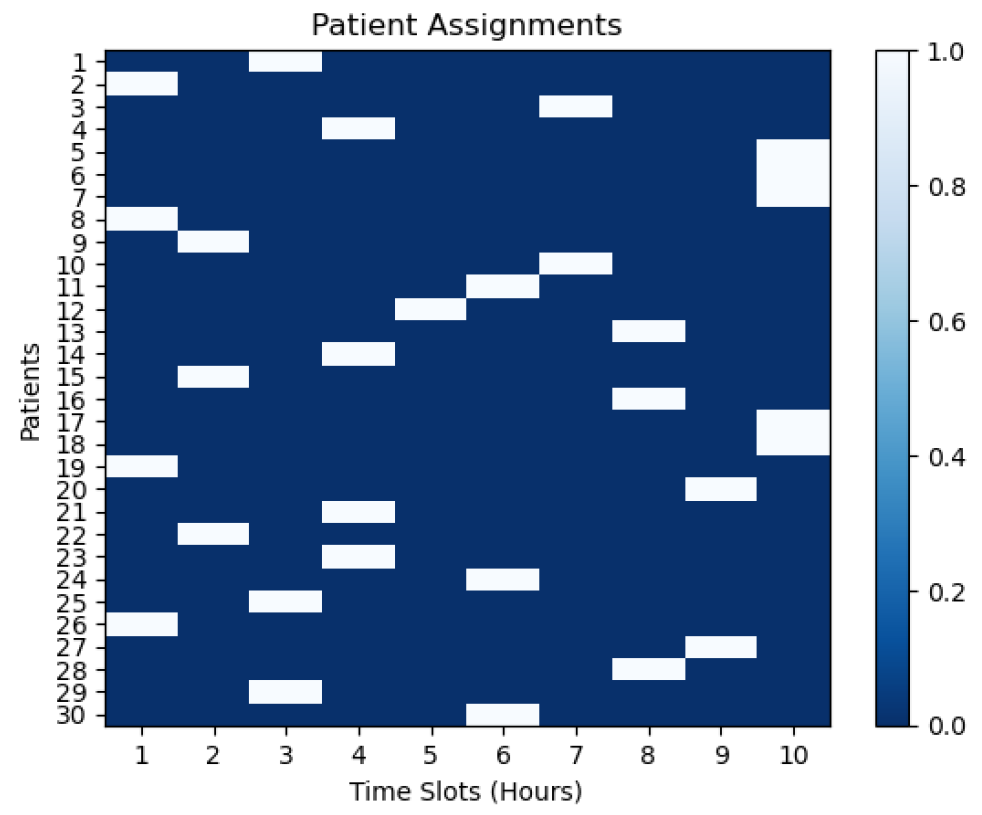
Let be a binary matrix, where i represents the index of patients, and j represents the index of time slots. if the patient is assigned to the time slot , and 0 otherwise.
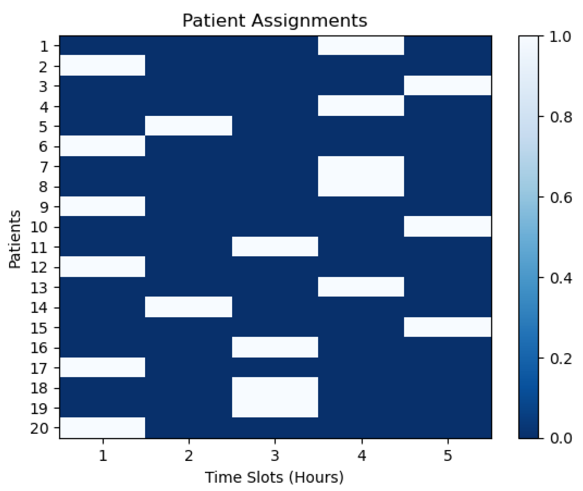
We observed patient time slots by using binary matrices for the two model procedures. Each matrix element of these two processes indicates whether a patient on the rows is assigned to a time slot on the columns. Afterward, we developed heat maps to display these data in Figure 7 and Figure 8. The heatmaps’ horizontal and vertical axes represent time slots and patients. The dark blue color-coded visualizations in the figures display patient assignments over time. The right-hand legends on the heatmaps, on a scale of 0.0 to 1.0, indicate the percentage of patients assigned at each time slot. For example, if the scale shows 0.7 at a specific time slot, this means that 70% of the patients are assigned at that time slot. The dark blue cells indicate assignments, whereas white cells indicate no patient assignments. In Figure 7, the 5 h time slot has the highest number of patient assignments, while in Figure 8, the 2 h time slot has the highest number of patient assignments.
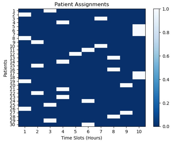
Figure 7.
Patient assignment for the first model procedure.
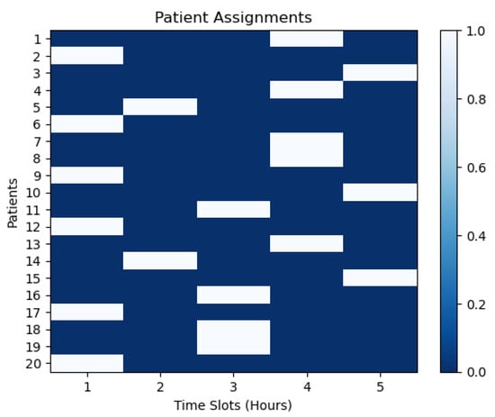
Figure 8.
Patient assignment for the second model procedure.
5.5. Actual and Maximum Allowed Working Hours
The total actual working hours, , for each staff member , is calculated as the sum of the product of a decision variable and a scale factor , with overall time slots . Here, could represent whether staff member i is working at time slot t, and could be a scale factor, such as the number of hours staff member i is expected to work.
Figure 9 and Figure 10 provide a visual representation of staff members’ actual working hours, categorized into regular (blue bars) and overtime hours (red bars). The x-axis enumerates the staff members, while the y-axis quantifies the working hours. In these visualizations, we compared the staff members’ actual and maximum work hours for the two model procedures. A dual-bar chart shows the outcomes for each staff member. Each pair’s blue bar signifies the staff member’s actual working hours. The red bars indicate the staff member’s maximum work hours. Moreover, this side-by-side comparison presents staff work-hour allocation and compliance. It also reveals possible disparities between actual work commitments and recommended maximum limitations, enabling optimal staff management. These depictions provide complete knowledge of staff use for resource allocation and management. By analyzing the distribution and contrast between regular and overtime hours, these figures are diagnostic tools to identify potential inefficiencies in staff scheduling and workload allocation. Also, the figures elucidate the balance between operational needs and compliance, facilitating targeted interventions where discrepancies are identified.
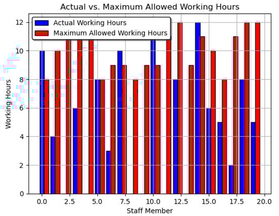
Figure 9.
Actual and maximum allowed working hours for the first model procedure.
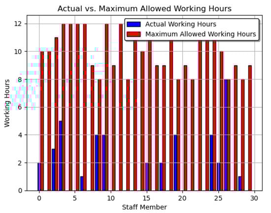
Figure 10.
Actual and maximum allowed working hours for the second model procedure.
5.6. Resource Utilization
- : A mapping of each resource to its utilization across all time slots.
- R: The set of resources, .
- T: The set of time slots.
- r: A specific resource from the set R.
- t: A specific time slot from the set T.
- : The utilization of resource r at time slot t, representing how much of that resource is being used or allocated at that specific time.
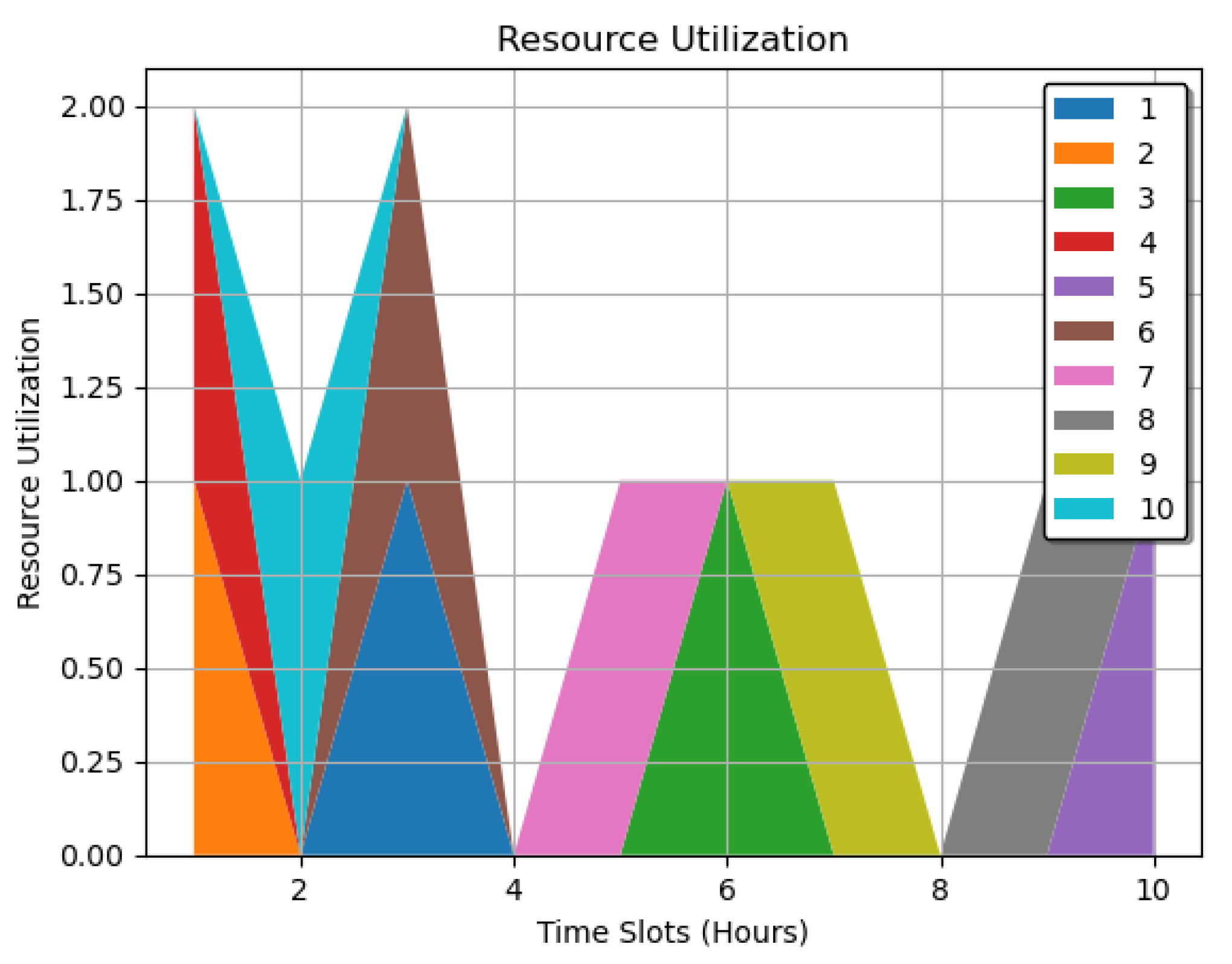
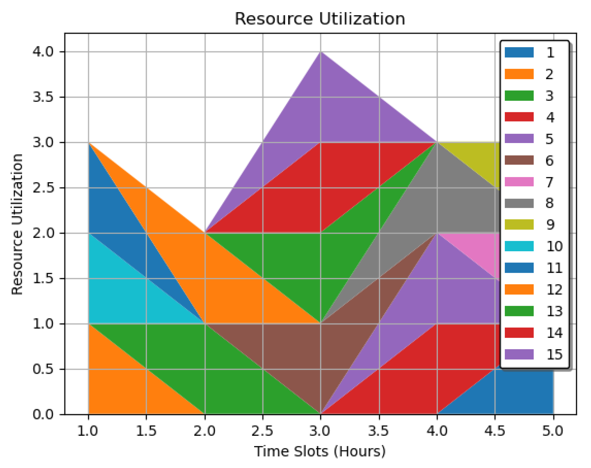
Figure 11 and Figure 12 offer a resource utilization analysis, employing different hues to signify various resource categories. The cumulative area under each hue quantifies the total utilization of the corresponding resource. We extensively studied resource utilization in the plots from 1 to 10 for the first procedure and 1 to 15 for the second procedure over specific periods. Then, we recorded each utilization to generate an in-depth profile. The stacked area plot in the graph displays time slots on the horizontal axes and resource utilization on the vertical axes for these procedures based on the resources allocated. Furthermore, the color-coded schemes depict the available resources, ranging from 1 to 10 in Figure 11 and 1 to 15 in Figure 12. The cumulative area beneath each hue shows resource utilization over time. Hence, the visualizations from the two figures reveal utilization differences between time slots in the system. The map-like process displays in the graphs also indicate resource-optimized time slots. The entire graphs assist in determining peak consumption and resource contentions for the optimization processes. By integrating both spatial and dimensional analysis, these plots show utilization trends and anomalies, supporting data-driven resource management strategies and optimizing resource allocation within the healthcare system.
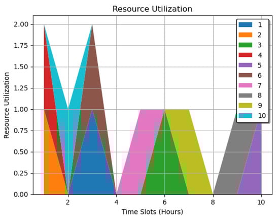
Figure 11.
Resource utilization over time slots for the first model procedure.
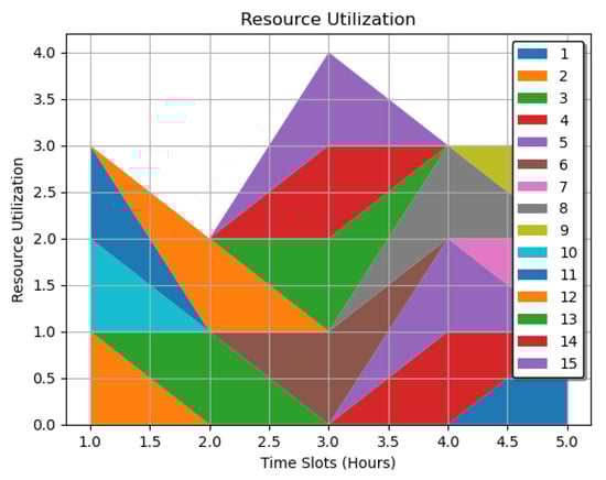
Figure 12.
Resource utilization over time slots for the second model procedure.
5.7. Patient and Staff Utilization
Patient and staff utilization represents the usage or allocation of resources for patients and staff overtime slots.
Patient Utilization:
- : Total number of assignments for all patients at each time slot.
- p: A specific patient within the set P.
- P: Refers to the collection of all patients.
- t: A specific time interval or slot within the set T.
- : Number of assignments for a particular patient at a given time slot.
- T: The collection of all time intervals or slots considered.
Staff Utilization:
- : Total number of assignments for all staff members at each time slot.
- i: A specific staff member within the set N.
- t: A specific time interval or slot within the set T.
- : Number of assignments for a particular staff member at a given time slot.
- N: The collection of all staff members.
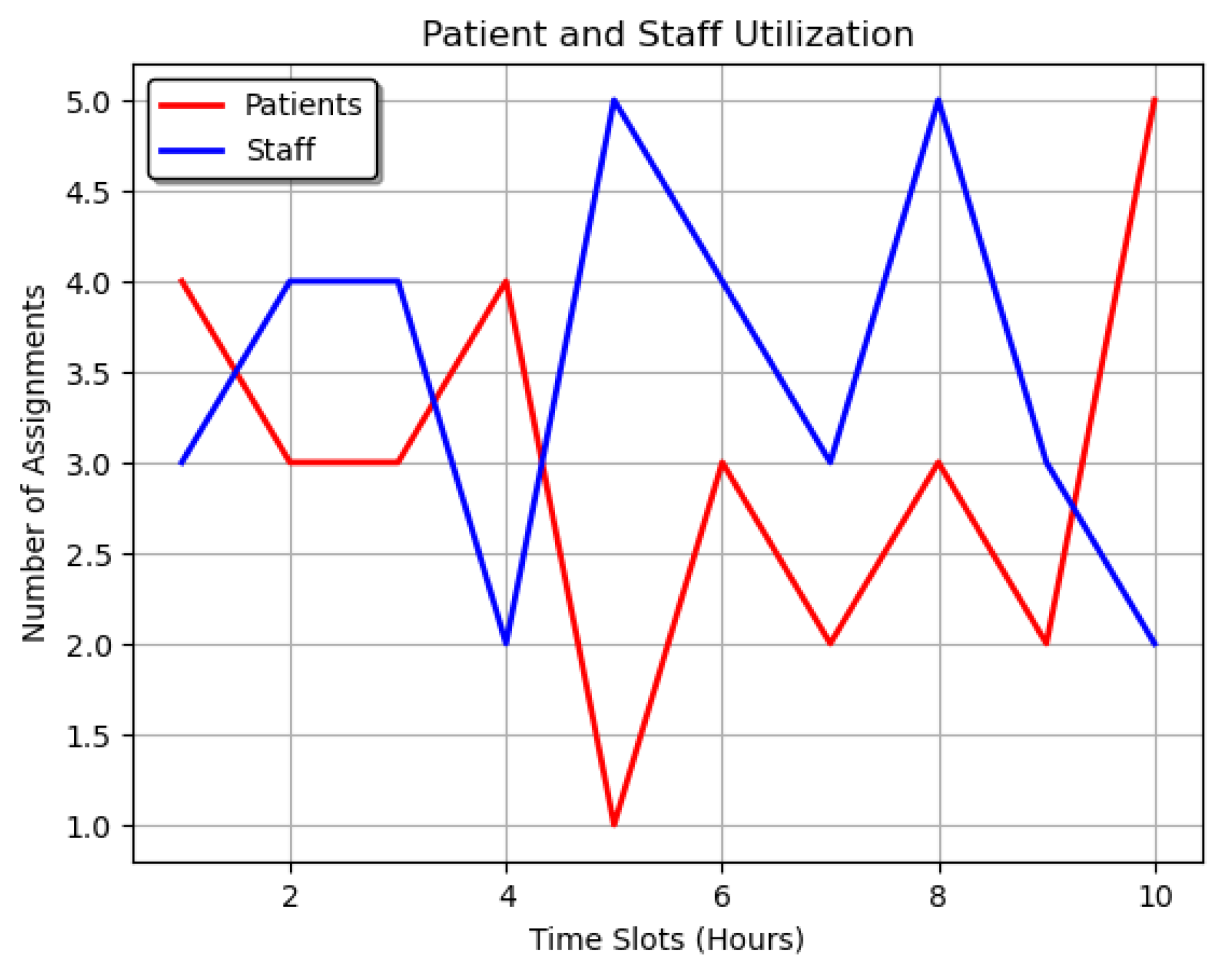
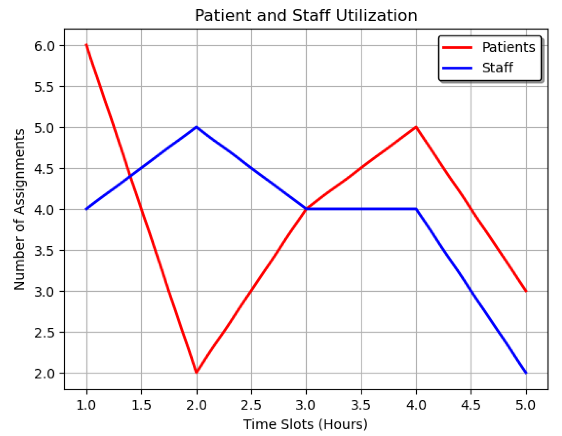
In Figure 13 and Figure 14, utilization refers to how many assignments each patient or staff member had in each time slot. These figures employ line graphs to depict staff assignments and the dynamics of task allocation over time. Red and blue lines correspond to specific roles or tasks, with intersections and divergences illustrating collaborative or independent work phases. We assessed these utilizations over time for both patients and staff. The graphs map each time slot to the model’s total number of patient and staff assignments for the two model scenarios. The line graphs display assignment changes over time. Furthermore, the patients have red lines, while the staff have blue ones. These visual distinctions make comparing the two utilizations easy. The graphs also reveal assignment patterns across time and between patients and staff. They also identify peak times and bottlenecks. The two processes optimize assignment allocation and boost healthcare operational efficiency. These line graphs synthesize complex scheduling data into a comprehensible format, allowing for in-depth analysis of staff deployment patterns, task synchronization, and inter-staff coordination.
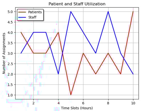
Figure 13.
Comparative analysis of patient and staff utilization over time for the first model procedure.
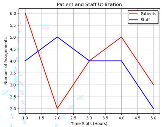
Figure 14.
Comparative analysis of patient and staff utilization over time for the second model procedure.
5.8. Demand and Capacity Analysis in Scheduling
We calculated and graphically presented each period’s total demand and capacity by scheduling patients P based on demand and the available capacity and at a set of periods T. We define and to denote total demand and capacity at time , respectively:
Here:
- Period’s Total Demand and Capacity: This refers to the overall demand and capacity for a specific period. It is calculated for scheduling patients based on available resources and demands.
- Patients P: This represents the set of all patients considered in the scheduling.
- Set of Periods T: This refers to the specific periods for which demand and capacity are calculated and scheduled.
- Demand at Time t, demandt: This is the total demand at a specific time t, calculated as the sum of the demand for all patients at that time. The demand for each patient p at time t is represented by .
- Capacity at Time t, capacityt: This is the total capacity at time t, calculated as the sum of a capacity-related variable for all patients at that time. The capacity-related variable for each patient p at time t is represented by .
- : This corresponds to the demand for a specific patient p at time t. It represents the patient’s required resources, treatment, or service.
- : This represents the value of a capacity-related variable for a specific patient p at time t. It may signify how much of a certain resource is allocated or available for that patient, possibly weighted by some variable x.
- (For All t in T): This notation signifies that the given equations for demand and capacity are applicable for all periods t in the set of periods T.
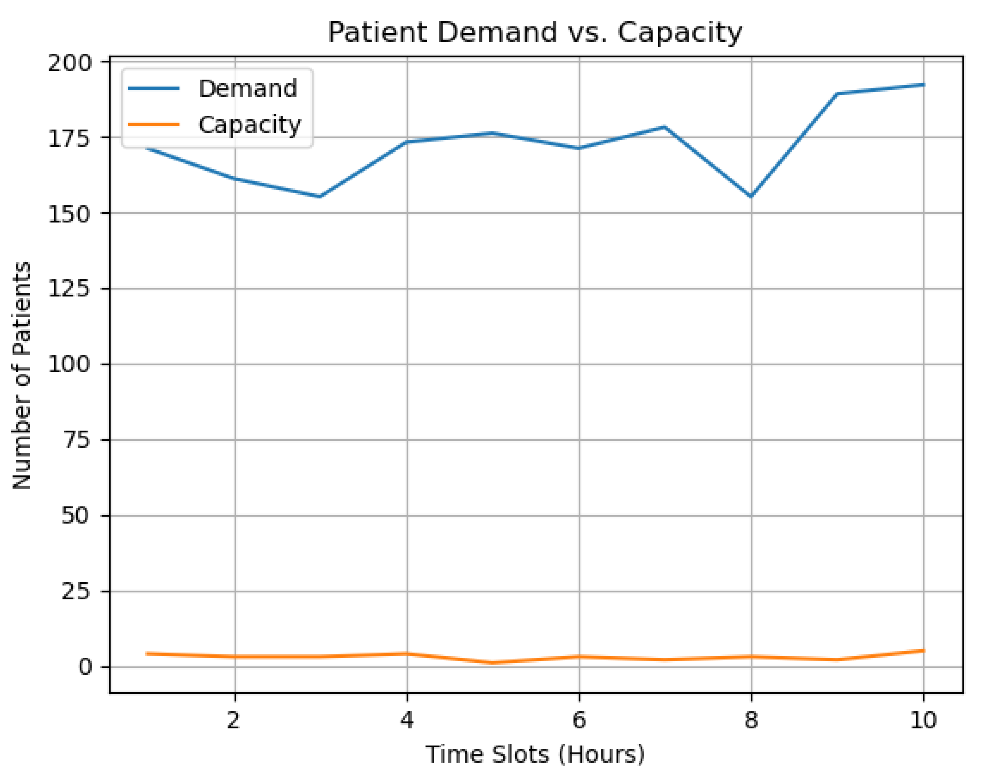
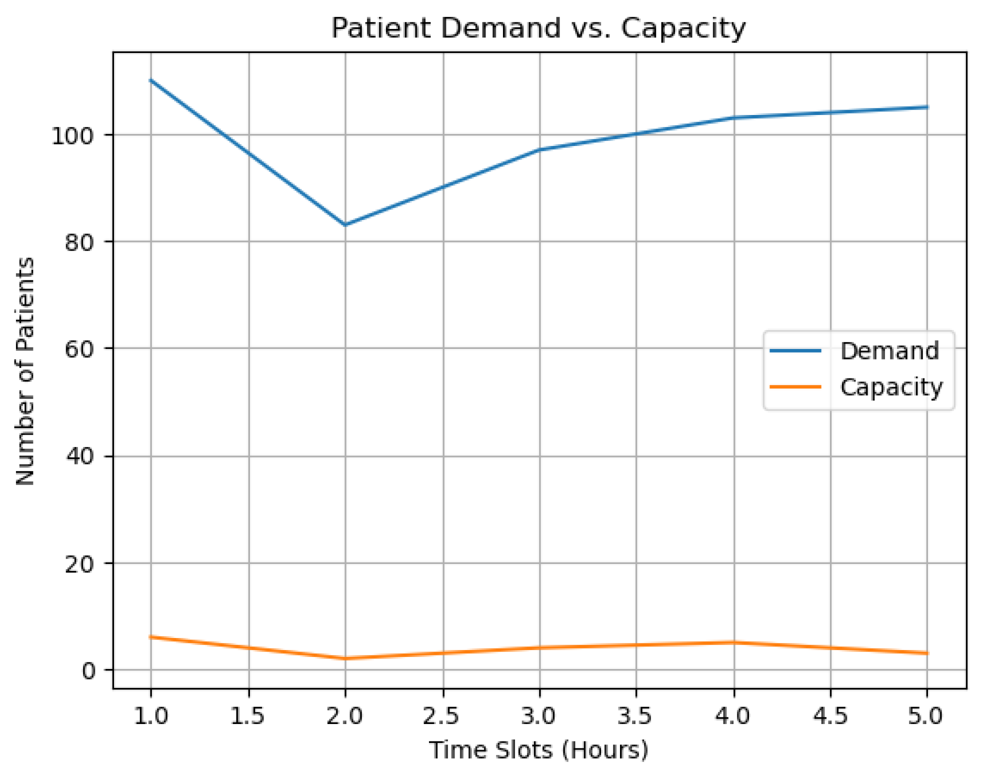
Patient demand and resource capacity are compared across time slots for the two model processes in Figure 15 and Figure 16. The plots offer several plausible outcomes. Demand exceeding capacity denotes a period when more resources are needed for patient care than are available. This imbalance can slow the delivery of patient care, necessitating steps to expand capacity or redistribute resources. On the other hand, a capacity line that is continuously above the demand line suggests that resources are not being used to their full potential and that reevaluating resource distribution might improve overall efficiency. Conversely, it indicates an ideal balance between patient requirements and available resources if the demand and capacity lines align or exhibit similar patterns. A careful examination of these trends can reveal tactical information to boost the effectiveness of patient scheduling. These figures employ geometric representations to describe the constraints, variables, and equations that define the optimization landscape. They contribute to the rigorous formulation of the problem, enhancing the understanding of the model’s structure, assumptions, and mathematical rigor.
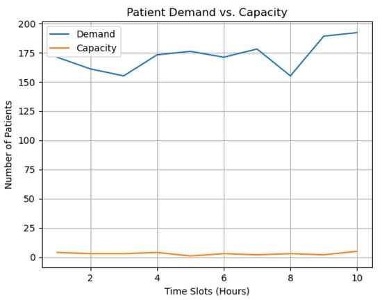
Figure 15.
Demand vs. capacity over time for the first model procedure.
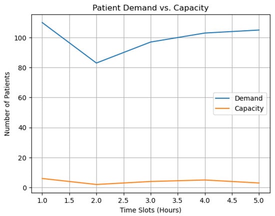
Figure 16.
Demand vs. capacity over time for the second model procedure.
5.9. Patient Satisfaction
Our model incorporates various variables including, but not limited to, patient satisfaction, staff interaction, conditional elements, patient utility, and other pertinent factors, all modeled using simulated data. Patient satisfaction in this model is derived from carefully aligning resources, staff, and patient needs within specific scheduling periods. By optimizing these elements in concert, we aim to create an environment that maximizes patient satisfaction, ensuring that resources are allocated to meet their requirements and expectations. We calculated patient satisfaction for each period . The patient satisfaction at time t, represented as , is computed as follows:
Here, denotes the utility of patient p, is the assignment variable corresponding to patient p being assigned to staff member i, and is a capacity-related variable for patient p at time t.
- Patient Satisfaction at Time t: satisfaction_t: This is the target variable representing the satisfaction level of patients at time t.
- Summation Over Patients and Staff: : This summation indicates that the calculation is done over all patients p in a set P and all staff members i in a set N.
- Conditional Part: : This condition implies that the summation is calculated only when the product of the capacity-related variable and some variable x is more significant than 0.5. This could be a threshold for considering only specific assignments or capacities.
- Utility of Patient p: : This represents the utility or benefit of a specific patient p, which may be based on their needs or preferences.
- Assignment Variable: : This term denotes the assignment of patient p to staff member i, possibly weighted by variable x. It might represent how well the staff member fits the patient’s needs.
- Denominator Summation: : This part sums up the capacity-related variable for all patients p in set P at time t. It likely represents the total capacity or availability at time t and is the normalizing factor for patient satisfaction.
- Main Equation: Putting all the parts together, the equation calculates patient satisfaction at time t as a weighted sum of utilities and assignments normalized by the total capacity-related variable.
Our results signified patient satisfaction as a function of time, illustrating staff allocation schemes’ effectiveness.
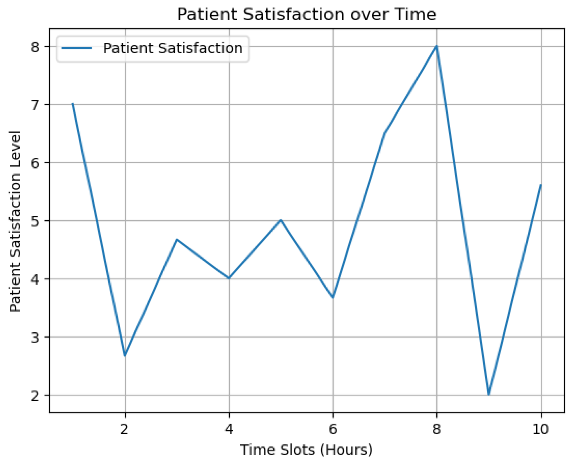
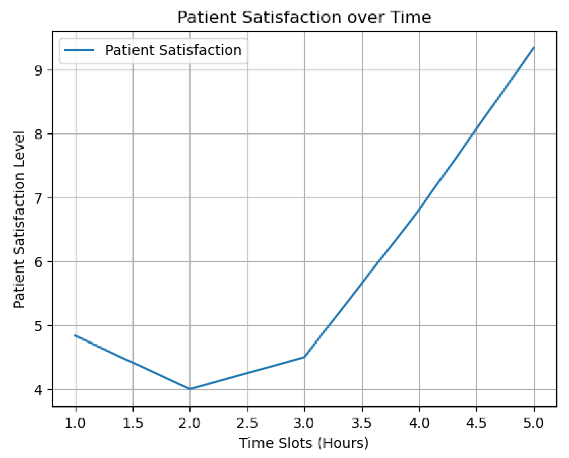
Figure 17 and Figure 18 plot patient satisfaction measures against time slots. They illustrate how staff allocation strategies affect patient satisfaction, emphasizing the importance of our results in improving healthcare delivery quality and the patient experience. The horizontal axes show time slots, while the vertical axes show the patient satisfaction measure for each period as an average weighted utility value for the two model procedures. High points on the graph indicate staff allocation efficacy due to appropriate personnel levels or expertise matching patient demands. Conversely, low numbers suggest inefficient personnel deployment. The plotted lines show gaps when the satisfaction metric is ambiguous owing to patient assignments. These graphs encapsulate a complex analysis of patient feedback, employing regression or curve-fitting techniques to infer underlying patterns. They are strategic tools for assessing patient experience, guiding scheduling decisions, and informing quality improvement initiatives.
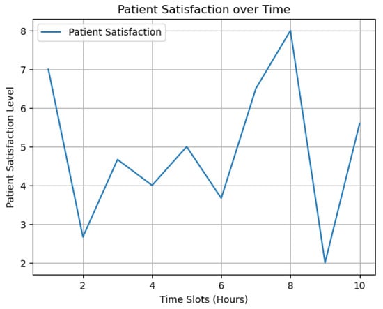
Figure 17.
Patient satisfaction over time for the first model procedure.

Figure 18.
Patient satisfaction over time for the second model procedure.
6. Conclusions
The primary concerns facing the healthcare sector are improving patient care, simplifying healthcare operations, and providing top-notch services at affordable costs. These challenges include general healthcare management, resource allocation, hiring, patient care priorities, and efficient scheduling. Effective staff scheduling, resource allocation, and patient assignments are needed to overcome these difficulties. To this end, we developed an MILP model using the Gurobi optimization solver to address these issues, thereby arriving at the desired results. The model encapsulates healthcare operations such as staff deployment, patient distribution, resource utilization, and monitoring overtime hours to enhance medical care and minimize expenditures.
Our model was implemented in two distinct scenarios, culminating in optimal solutions. For the first experimental implementation, we achieved an objective value of 844.0; for the second procedure, we obtained an objective value of 539.0. Despite the differing contexts, both performances resulted in a 0.0% gap, signifying an excellent alignment between the top solutions and the theoretical minima of the objective function. This, in turn, underscores the precision and effectiveness of our approach, which builds upon previous studies in healthcare scheduling and management. Furthermore, our model offers healthcare organizations a valuable tool for managing finite resources and proactively reducing patient wait times. This aspect promises to enhance operational efficiency and patient outcomes.
The academic implications of our study lie in developing a novel MILP model tailored to the unique challenges of healthcare resource allocation and scheduling. By integrating the specific parameters of staff, resources, and patient demands, we contribute to the ongoing academic discourse on healthcare optimization, offering a new perspective and methodological approach. The managerial implications are directly related to the practical application of our model within healthcare settings. Our research offers a systematic and adaptable resource allocation and scheduling framework, allowing healthcare managers to improve patient care, simplify operations, and control costs more effectively. The model provides actionable insights that can be translated into real-world strategies, enhancing operational efficiency and patient satisfaction.
7. Future Research Directions
In future work, we will enhance the model’s performance, versatility, and adaptability by incorporating data from hospital settings, building on the present work. This process will offer a more accurate and contextually sensitive basis for improvement. Another significant research area is introducing uncertainty and unpredictability into the model. Under dynamic and unexpected operational situations, this refinement keeps the optimization approach successful. Furthermore, we will incorporate unexpected patient demand or staff absences into the model, resulting in more robustness. Future research should evaluate the model’s efficacy in diverse healthcare settings, such as emergency rooms and outpatient clinics. The model will also be tested and validated in different healthcare delivery situations and processes to improve its generalizability and practicality. Integrating the model with additional healthcare technology will explore synergies. For example, electronic health records and telemedicine are potential data sources and operational interfaces that can optimize the model. Hence, these methods enhance the model’s ability to improve healthcare resource management.
Author Contributions
Conceptualization, A.Y. and M.F.; methodology, A.Y. and M.F.; software, A.Y. and M.F.; validation, A.Y. and M.F.; formal analysis, A.Y. and M.F.; investigation, A.Y. and M.F.; resources, A.Y. and M.F.; data curation, A.Y. and M.F.; writing—original draft preparation, A.Y. and M.F.; writing—review and editing, A.Y. and M.F.; visualization, A.Y. and M.F.; supervision, M.F.; project administration, M.F. All authors have read and agreed to the published version of the manuscript.
Funding
This research received no external funding.
Institutional Review Board Statement
Not applicable.
Informed Consent Statement
Not applicable.
Data Availability Statement
The article contains the supporting data necessary to understand the findings of this study. To simulate realistic healthcare scheduling constraints, the numerical values employed in this study were created within preset ranges. However, this study is based on simulated data rather than actual patient or hospital data, so it can only be directly applied to specific healthcare scenarios with modifications.
Conflicts of Interest
The authors declare no conflict of interest.
Abbreviations
The following abbreviations are used in this manuscript:
| MILP | Mixed-Integer Linear Programming |
| LP | Linear Programming |
References
- Hughes, R.G. Tools and strategies for quality improvement and patient safety. In Patient Safety and Quality: An Evidence-Based Handbook for Nurses; Agency for Healthcare Research and Quality: Rockville, MD, USA, 2008. [Google Scholar]
- Yen, P.Y.; Kellye, M.; Lopetegui, M.; Saha, A.; Loversidge, J.; Chipps, E.M.; Gallagher-Ford, L.; Buck, J. Nurses’ time allocation and multitasking of nursing activities: A time motion study. In AMIA Annual Symposium Proceedings; American Medical Informatics Association: Bethesda, MD, USA, 2018; Volume 2018, p. 1137. [Google Scholar]
- Dugdale, D.C.; Epstein, R.; Pantilat, S.Z. Time and the patient-physician relationship. J. Gen. Intern. Med. 1999, 14, S34. [Google Scholar] [CrossRef] [PubMed]
- Mosadeghrad, A.M. Factors influencing healthcare service quality. Int. J. Health Policy Manag. 2014, 3, 77. [Google Scholar] [CrossRef] [PubMed]
- How to Ease the Nursing Shortage in America. Available online: https://www.americanprogress.org/article/how-to-ease-the-nursing-shortage-in-america/ (accessed on 24 August 2023).
- Haleem, A.; Javaid, M.; Singh, R.P.; Suman, R. Telemedicine for healthcare: Capabilities, features, barriers, and applications. Sens. Int. 2021, 2, 100117. [Google Scholar] [CrossRef] [PubMed]
- Holmér, S.; Nedlund, A.C.; Thomas, K.; Krevers, B. How health care professionals handle limited resources in primary care–an interview study. BMC Health Serv. Res. 2023, 23, 1–12. [Google Scholar] [CrossRef]
- Rahardja, U.; Andriyani, F.; Triyono, T. Model Scheduling Optimization Workforce Management Marketing. APTISI Trans. Manag. (ATM) 2020, 4, 92–100. [Google Scholar] [CrossRef]
- Moussavi, S.E.; Mahdjoub, M.; Grunder, O. A matheuristic approach to the integration of worker assignment and vehicle routing problems: Application to home healthcare scheduling. Expert Syst. Appl. 2019, 125, 317–332. [Google Scholar] [CrossRef]
- Afshar-Nadjafi, B. Multi-skilling in scheduling problems: A review on models, methods and applications. Comput. Ind. Eng. 2021, 151, 107004. [Google Scholar] [CrossRef]
- Abdalkareem, Z.A.; Amir, A.; Al-Betar, M.A.; Ekhan, P.; Hammouri, A.I. Healthcare scheduling in optimization context: A review. Health Technol. 2021, 11, 445–469. [Google Scholar] [CrossRef]
- García-Nieves, J.D.; Ponz-Tienda, J.L.; Ospina-Alvarado, A.; Bonilla-Palacios, M. Multipurpose linear programming optimization model for repetitive activities scheduling in construction projects. Autom. Constr. 2019, 105, 102799. [Google Scholar] [CrossRef]
- Ghannam, L. Development of a Mathematical Model for Optimal Scheduling of Patients and Resource Management in Healthcare in Palestine during the Pandemic. Ph.D. Thesis, An-Najah National University, Nablus, Palestine, 2022. [Google Scholar]
- Ala, A.; Goli, A.; Nejad Attari, M.Y. Scheduling and routing of dispatching medical staff to homes healthcare from different medical centers with considering fairness policy. Math. Probl. Eng. 2022, 2022, 3189574. [Google Scholar] [CrossRef]
- Guastalla, A.; Sulis, E.; Aringhieri, R.; Branchi, S.; Di Francescomarino, C.; Ghidini, C. Workshift scheduling using optimization and process mining techniques: An application in healthcare. In Proceedings of the 2022 Winter Simulation Conference (WSC), Singapore, 11–14 December 2022; IEEE: Piscataway, NJ, USA, 2022; pp. 1116–1127. [Google Scholar]
- Maghzi, P.; Roohnavazfar, M.; Mohammadi, M.; Naderi, B. A Mathematical Model for Operating Room Scheduling Considering Limitations on Human Resources Access and Patient Prioritization. J. Qual. Eng. Prod. Optim. 2019, 4, 67–82. [Google Scholar]
- Mielczarek, B. Review of modelling approaches for healthcare simulation. Oper. Res. Decis. 2016, 26. [Google Scholar]
- Yinusa, A.; Faezipour, M.; Faezipour, M. A Study on CKD Progression and Health Disparities Using System Dynamics Modeling. Healthcare 2022, 10, 1628. [Google Scholar] [CrossRef] [PubMed]
- Maenhout, B.; Vanhoucke, M. An integrated nurse staffing and scheduling analysis for longer-term nursing staff allocation problems. Omega 2013, 41, 485–499. [Google Scholar] [CrossRef]
- Restrepo, M.I.; Rousseau, L.M.; Vallée, J. Home healthcare integrated staffing and scheduling. Omega 2020, 95, 102057. [Google Scholar] [CrossRef]
- Granja, C.; Almada-Lobo, B.; Janela, F.; Seabra, J.; Mendes, A. An optimization based on simulation approach to the patient admission scheduling problem using a linear programing algorithm. J. Biomed. Inform. 2014, 52, 427–437. [Google Scholar] [CrossRef] [PubMed]
- Ala, A.; Alsaadi, F.E.; Ahmadi, M.; Mirjalili, S. Optimization of an appointment scheduling problem for healthcare systems based on the quality of fairness service using whale optimization algorithm and NSGA-II. Sci. Rep. 2021, 11, 19816. [Google Scholar] [CrossRef]
- Bennett, A.R.; Erera, A.L. Dynamic periodic fixed appointment scheduling for home health. IIE Trans. Healthc. Syst. Eng. 2011, 1, 6–19. [Google Scholar] [CrossRef]
- Leksakul, K.; Phetsawat, S. Nurse scheduling using genetic algorithm. Math. Probl. Eng. 2014, 2014. [Google Scholar] [CrossRef]
- Turhan, A.M.; Bilgen, B. Mixed integer programming based heuristics for the patient admission scheduling problem. Comput. Oper. Res. 2017, 80, 38–49. [Google Scholar] [CrossRef]
- Bolaji, A.L.; Bamigbola, A.F.; Adewole, L.B.; Shola, P.B.; Afolorunso, A.; Obayomi, A.A.; Aremu, D.R.; Almazroi, A.A.A. A room-oriented artificial bee colony algorithm for optimizing the patient admission scheduling problem. Comput. Biol. Med. 2022, 148, 105850. [Google Scholar] [CrossRef] [PubMed]
- Bastos, L.S.; Marchesi, J.F.; Hamacher, S.; Fleck, J.L. A mixed integer programming approach to the patient admission scheduling problem. Eur. J. Oper. Res. 2019, 273, 831–840. [Google Scholar] [CrossRef]
- Gocgun, Y.; Bresnahan, B.W.; Ghate, A.; Gunn, M.L. A Markov decision process approach to multi-category patient scheduling in a diagnostic facility. Artif. Intell. Med. 2011, 53, 73–81. [Google Scholar] [CrossRef] [PubMed]
- Li, H.; Li, X.; Gao, L. A discrete artificial bee colony algorithm for the distributed heterogeneous no-wait flowshop scheduling problem. Appl. Soft Comput. 2021, 100, 106946. [Google Scholar] [CrossRef]
- Gurobi Optimization. Available online: https://www.gurobi.com (accessed on 24 August 2023).


Disclaimer/Publisher’s Note: The statements, opinions and data contained in all publications are solely those of the individual author(s) and contributor(s) and not of MDPI and/or the editor(s). MDPI and/or the editor(s) disclaim responsibility for any injury to people or property resulting from any ideas, methods, instructions or products referred to in the content. |
© 2023 by the authors. Licensee MDPI, Basel, Switzerland. This article is an open access article distributed under the terms and conditions of the Creative Commons Attribution (CC BY) license (https://creativecommons.org/licenses/by/4.0/).