
A Distinctive Explainable Machine Learning Framework for Detection of Polycystic Ovary Syndrome

 ,
,  , ,
, ,
Abstract
1. Introduction
2. Literature Review
3. Materials and Methods
3.1. Dataset Description
3.2. Data Pre-Processing
3.3. Feature Selection
3.3.1. Harris Hawks Optimization (HHO)
3.3.2. Salp Swarm Optimization (SSA)
3.3.3. Mutual Information (MI)
4. Results
4.1. Performance Metrics
4.2. Model Evaluation with Machine Learning
4.3. Model Evaluation using Deep Learning
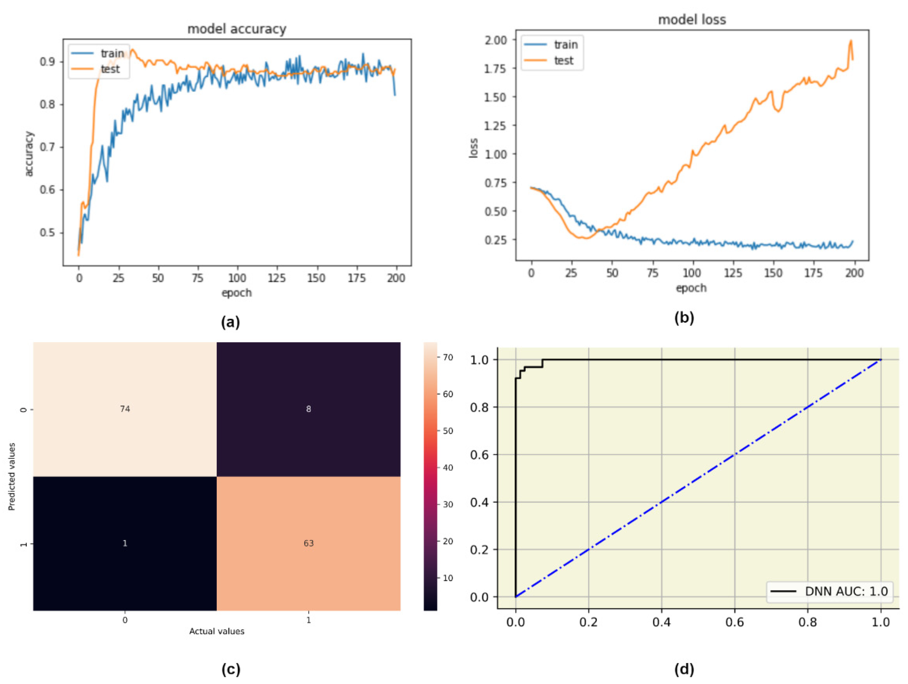
4.3.1. Deep Neural Network (DNN)
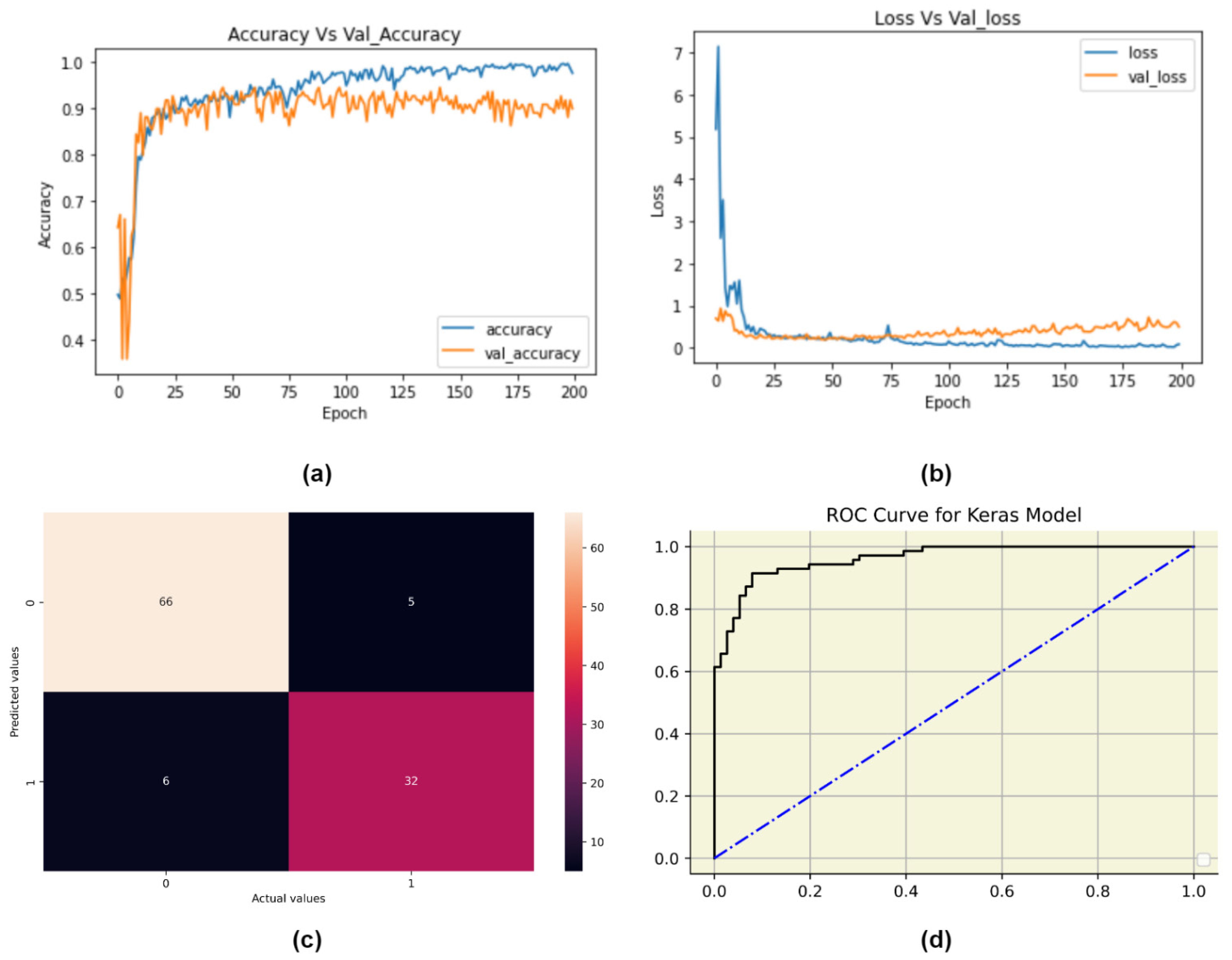
4.3.2. 1-Dimensional Convolutional Neural Network (1D-CNN)
4.4. Explainable AI (XAI)
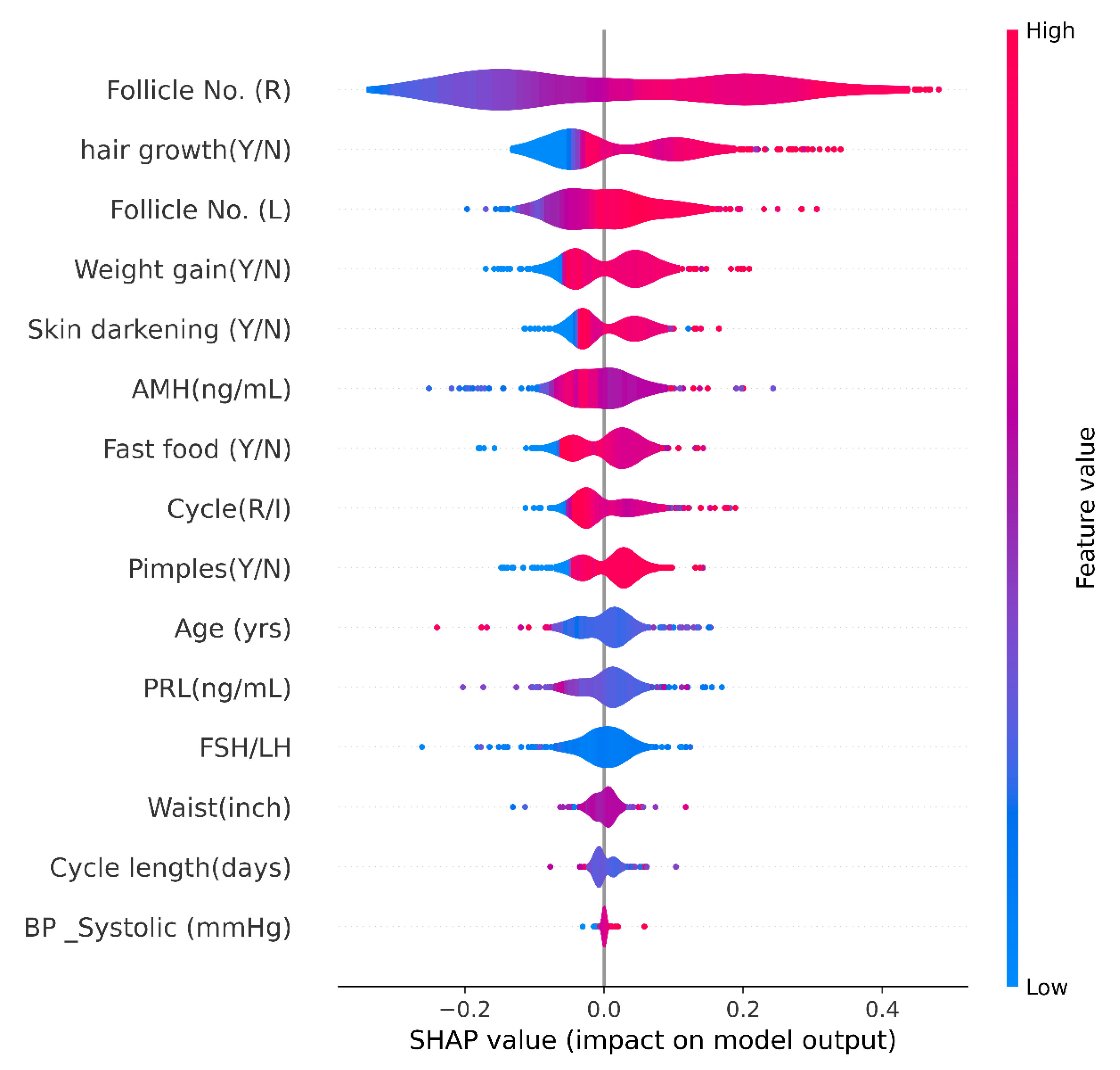
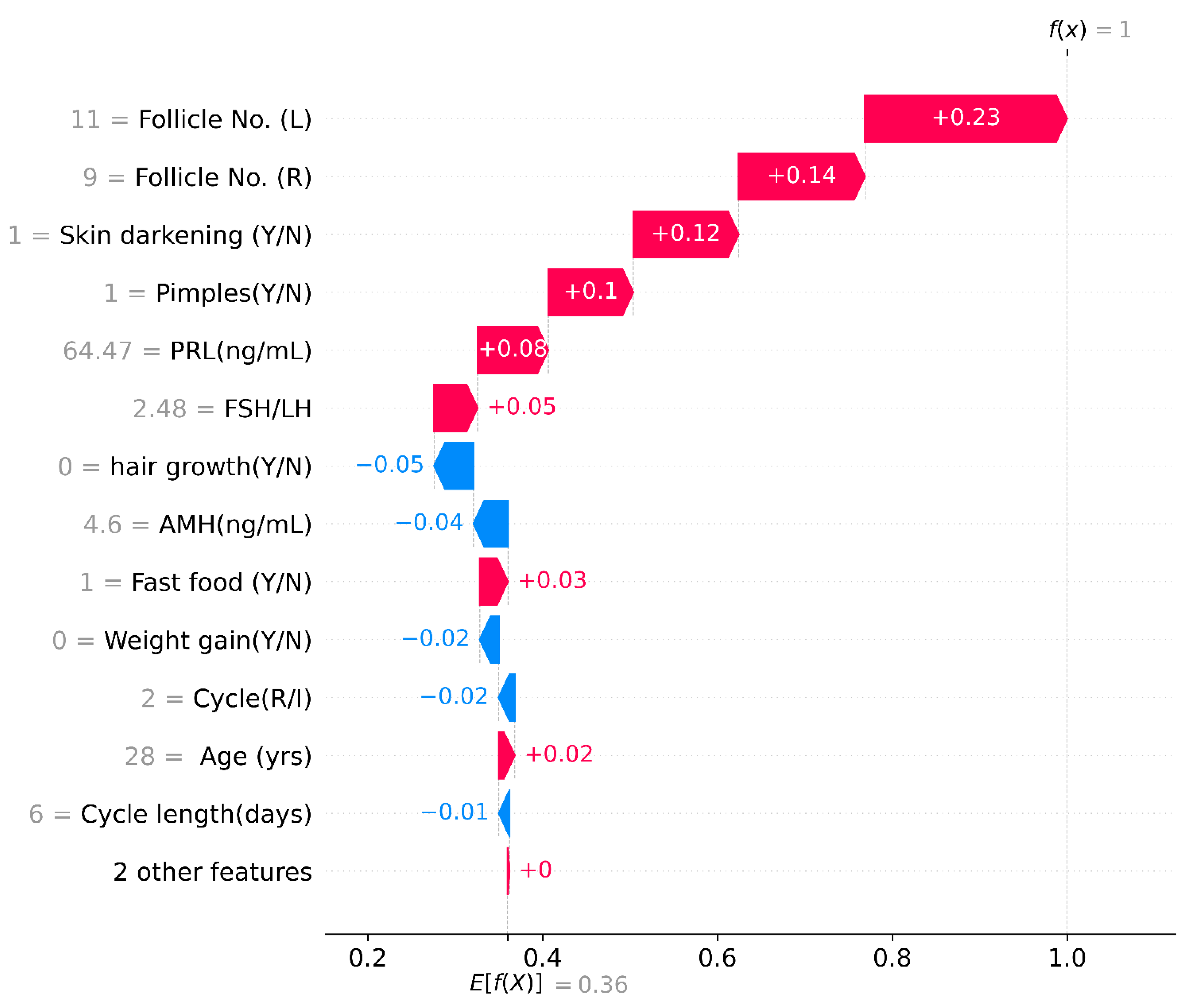
4.4.1. Shapley Additive exPlanations (SHAP)
SHAP Violin Plot
SHAP Waterfall Plot
SHAP Force Plot
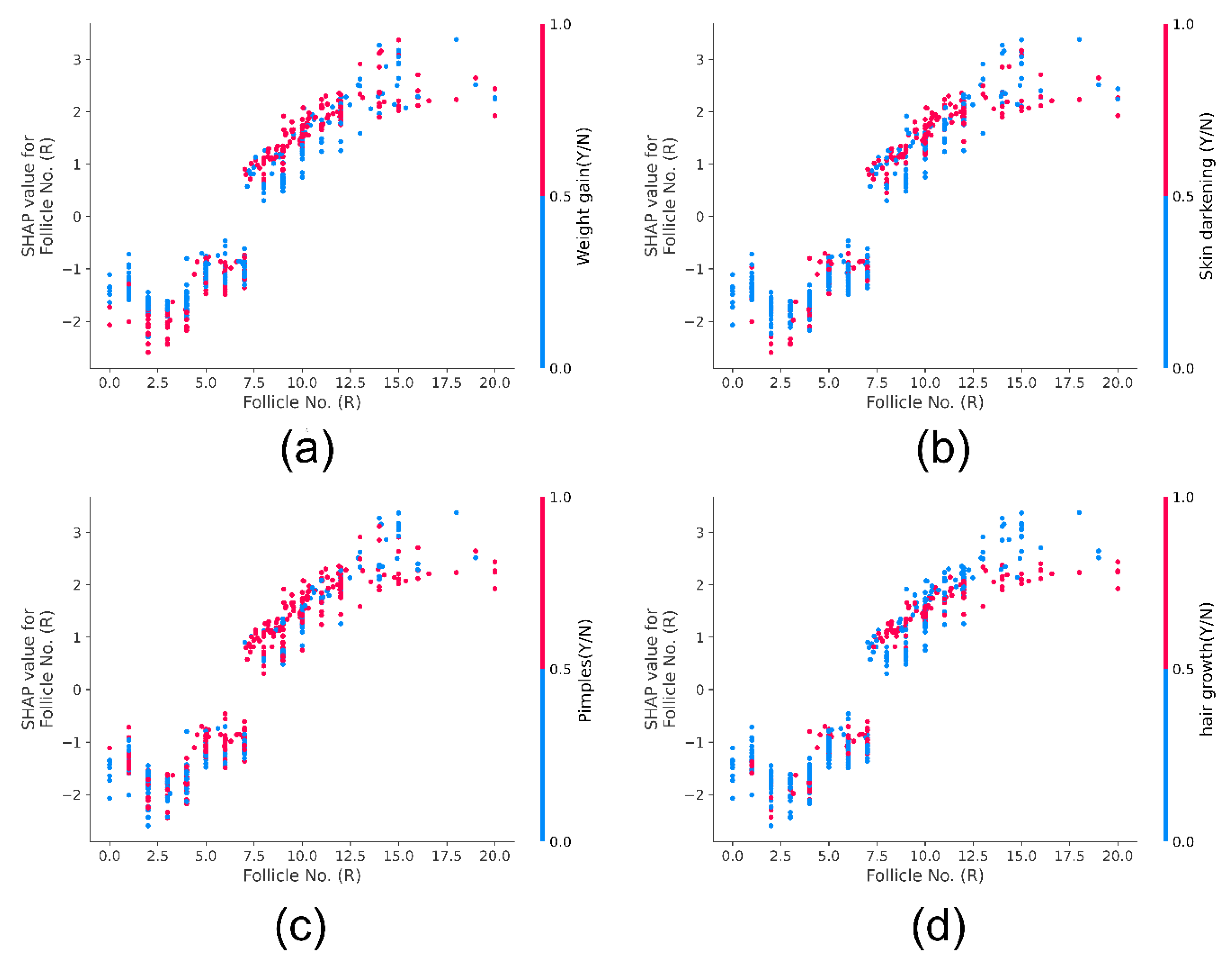
SHAP Dependance Plot
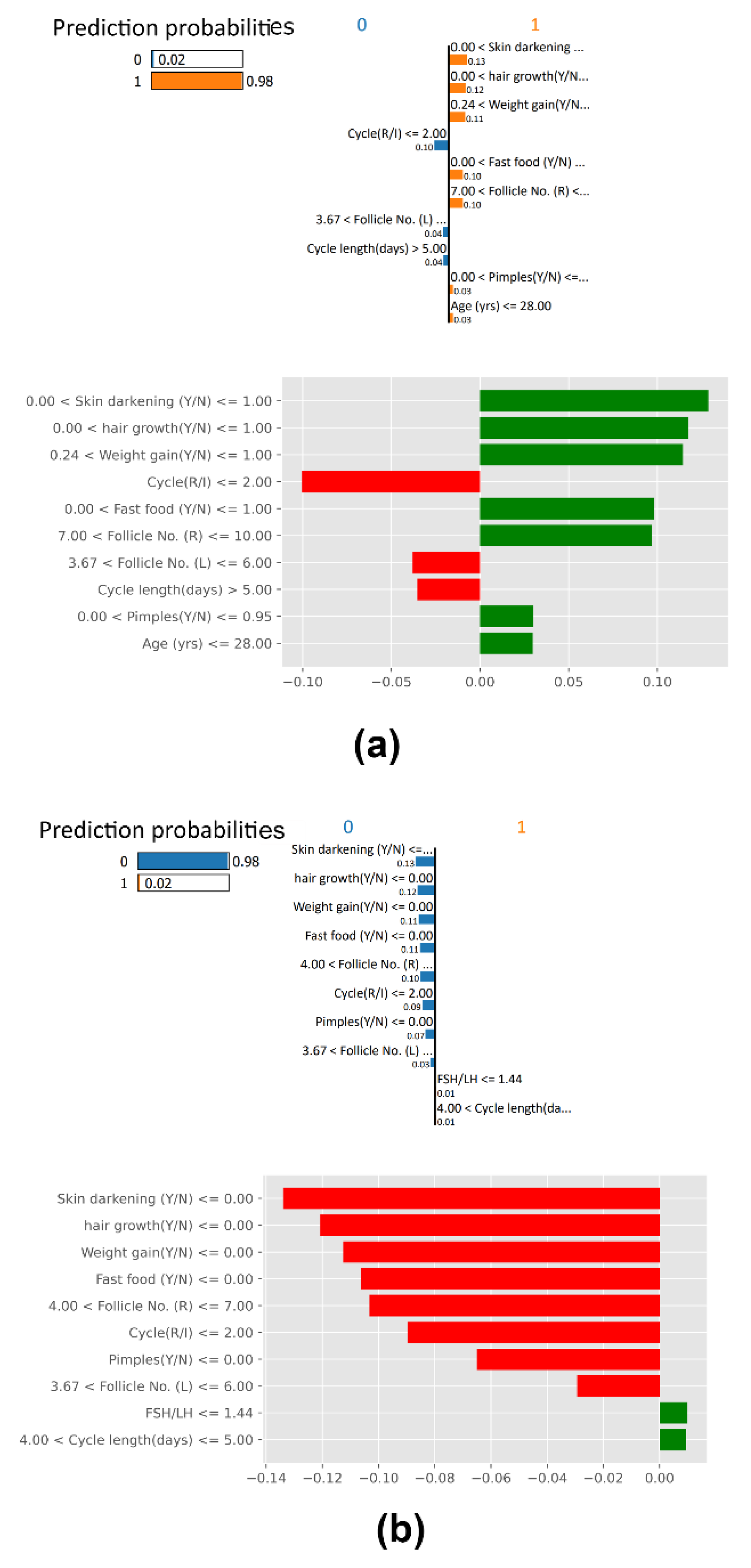
4.4.2. Local Interpretable Model-Agnostic Explanations (LIME)
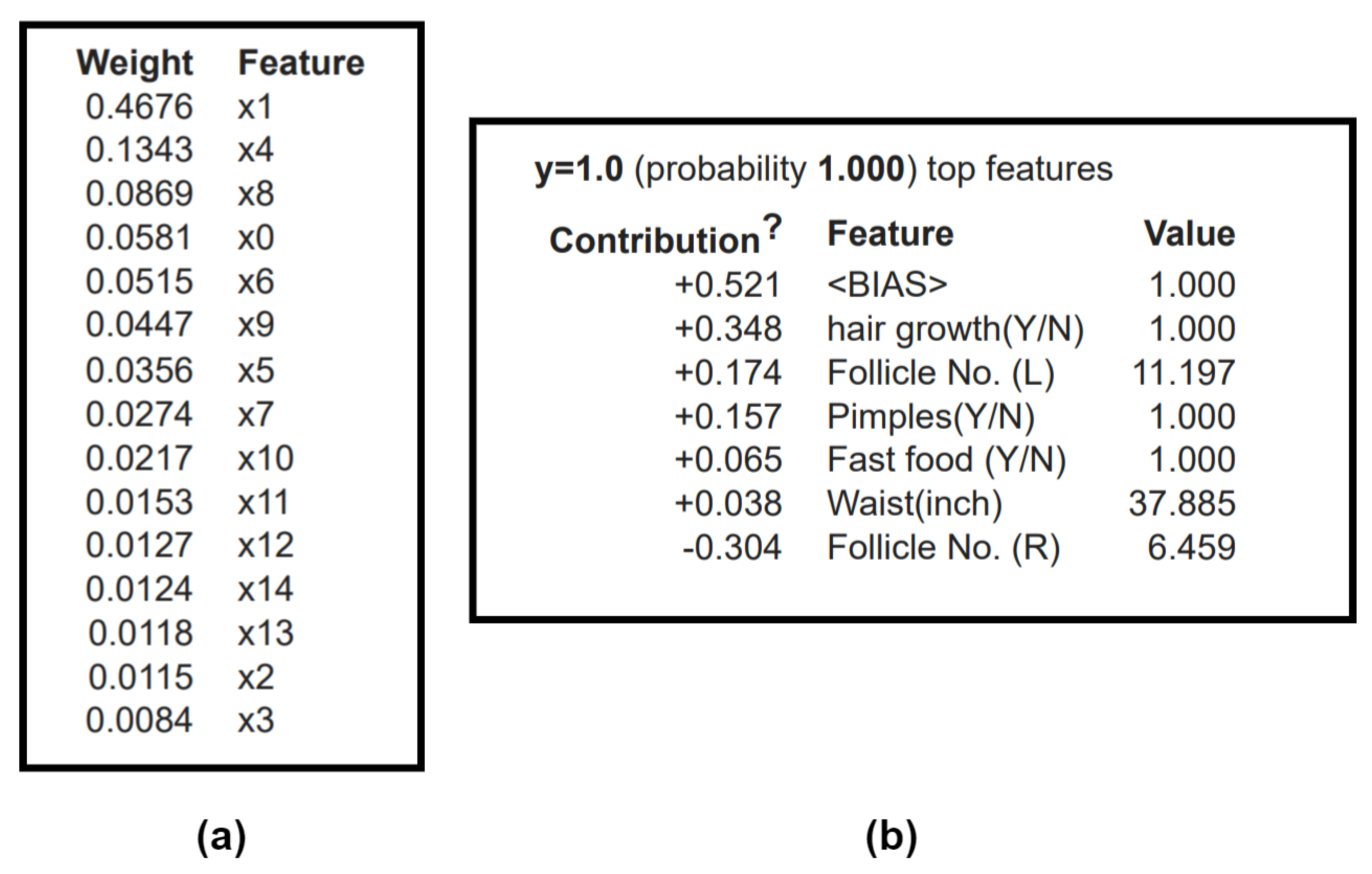
4.4.3. ELI5
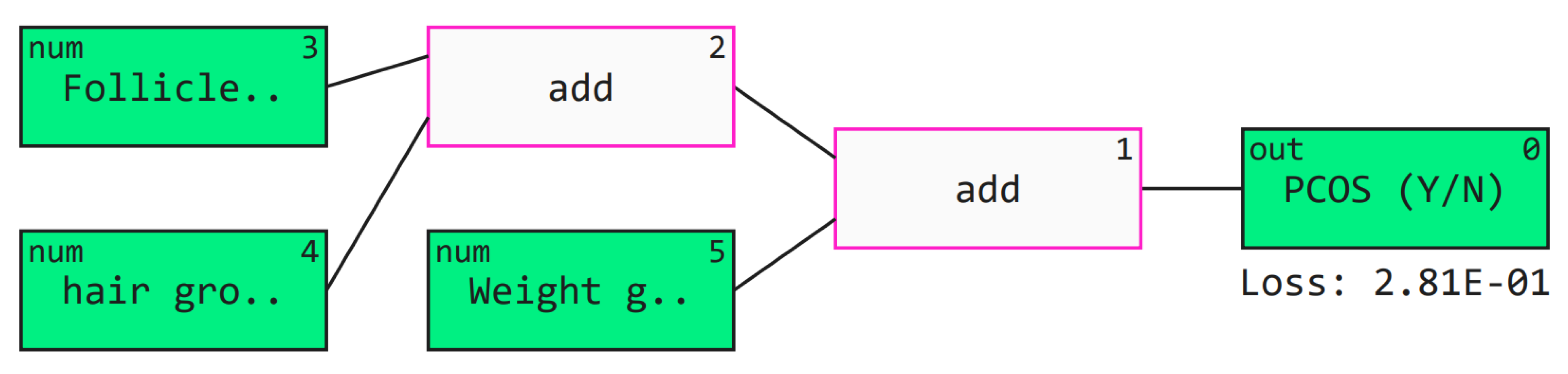
4.4.4. QLattice
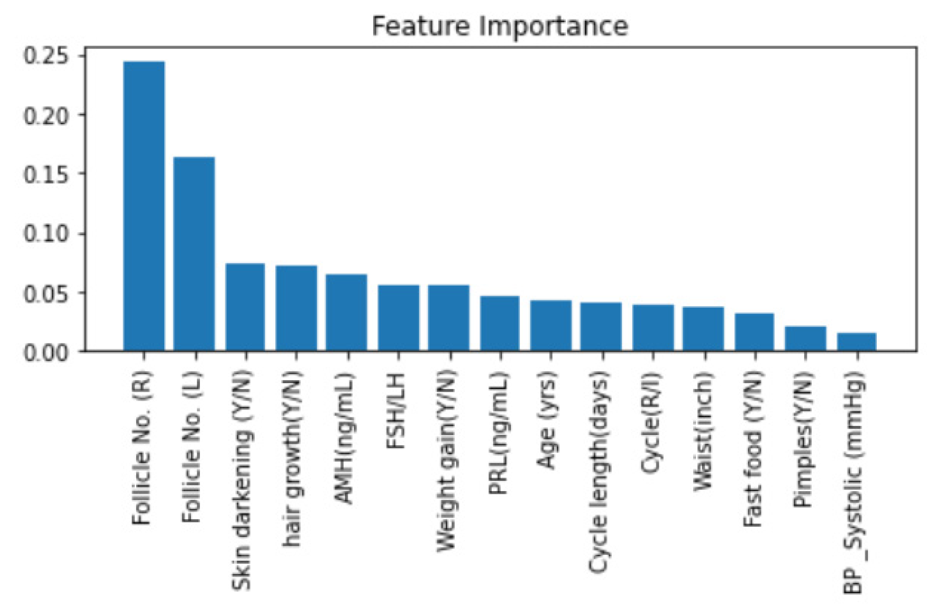
4.4.5. Feature Importance with Random Forest
5. Discussion
6. Conclusions and Future Scope
Author Contributions
Funding
Data Availability Statement
Conflicts of Interest
References
- Azziz, R.; Carmina, E.; Dewailly, D.; Diamanti-Kandarakis, E.; Escobar-Morreale, H.F.; Futterweit, W.; Janssen, O.E.; Legro, R.S.; Norman, R.; Taylor, A.E.; et al. The Androgen Excess and PCOS Society criteria for the polycystic ovary syndrome: The complete task force report. Fertil. Steril. 2009, 91, 456–488. [Google Scholar] [CrossRef] [PubMed]
- Ndefo, U.A.; Eaton, A.; Green, M.R. Polycystic ovary syndrome: A review of treatment options with a focus on pharmacological approaches. Pharm. Ther. 2013, 38, 336. [Google Scholar]
- Mohan, V.; Mehreen, T.S.; Ranjani, H.; Kamalesh, R.; Ram, U.; Anjana, R.M. Prevalence of polycystic ovarian syndrome among adolescents and young women in India. J. Diabetol. 2021, 12, 319–325. [Google Scholar] [CrossRef]
- Rojhani, E.; Rahmati, M.; Firouzi, F.; Saei Ghare Naz, M.; Azizi, F.; Ramezani Tehrani, F. Polycystic Ovary Syndrome, Subclinical Hypothyroidism, the Cut-Off Value of Thyroid Stimulating Hormone; Is There a Link? Findings of a Population-Based Study. Diagnostics 2023, 13, 316. [Google Scholar] [CrossRef] [PubMed]
- Mcdonald, T.W.; Malkasian, G.D.; Gaffey, T.A. Endometrial cancer associated with feminizing ovarian tumor and polycystic ovarian disease. Obstet. Gynecol. 1977, 49, 654–658. [Google Scholar] [CrossRef] [PubMed]
- Diamanti-Kandarakis, E.; Christakou, C.D. Insulin resistance in PCOS. Diagn. Manag. Polycystic Ovary Syndr. 2009, 35–61. [Google Scholar] [CrossRef]
- Schorr, H.; Rappaport, A. Innovative Applications of Artificial Intelligence; AAAI Press: Cambridge, UK, 1989. [Google Scholar]
- Benke, K.; Benke, G. Artificial intelligence and big data in public health. Int. J. Environ. Res. Public Health 2018, 15, 2796. [Google Scholar] [CrossRef]
- Szolovits, P.; Patil, R.S.; Schwartz, W.B. Artificial intelligence in medical diagnosis. Ann. Intern. Med. 1988, 108, 80–87. [Google Scholar] [CrossRef]
- Tang, Y.M.; Zhang, L.; Bao, G.Q.; Ren, F.J.; Pedrycz, W. Symmetric implicational algorithm derived from intuitionistic fuzzy entropy. Iran. J. Fuzzy Syst. 2022, 19, 27–44. [Google Scholar]
- Tang, Y.; Pan, Z.; Pedrycz, W.; Ren, F.; Song, X. Based kernel fuzzy clustering with weight information granules. IEEE Trans. Emerg. Top. Comput. Intell. 2022, 1–15. [Google Scholar] [CrossRef]
- Mulyanto, M.; Faisal, M.; Prakosa, S.W.; Leu, J.S. Effectiveness of focal loss for minority classification in network intrusion detection systems. Symmetry 2021, 13, 4. [Google Scholar] [CrossRef]
- Chen, M.; Wei, Z.; Ding, B.; Li, Y.; Yuan, Y.; Du, X.; Wen, J.R. Scalable graph neural networks via bidirectional propagation. Adv. Neural Inf. Process. Syst. 2020, 33, 14556–14566. [Google Scholar]
- Bhardwaj, K.K.; Banyal, S.; Sharma, D.K. Artificial intelligence based diagnostics, therapeutics and applications in biomedical engineering and bioinformatics. In Internet of Things in Biomedical Engineering; Academic Press: Cambridge, MA, USA, 2019; pp. 161–187. [Google Scholar]
- Liu, L.; Shen, F.; Liang, H.; Yang, Z.; Yang, J.; Chen, J. Machine Learning-Based Modeling of Ovarian Response and the Quantitative Evaluation of Comprehensive Impact Features. Diagnostics 2022, 12, 492. [Google Scholar] [CrossRef] [PubMed]
- Khanna, V.V.; Chadaga, K.; Sampathila, N.; Prabhu, S.; Chadaga, R.; Umakanth, S. Diagnosing COVID-19 using artificial intelligence: A comprehensive review. Netw. Model. Anal. Health Inform. Bioinform. 2022, 11, 1–23. [Google Scholar] [CrossRef]
- Chadaga, K.; Prabhu, S.; Sampathila, N.; Chadaga, R.; Ks, S.; Sengupta, S. Predicting cervical cancer biopsy results using demographic and epidemiological parameters: A custom stacked ensemble machine learning approach. Cogent Eng. 2022, 9, 2143040. [Google Scholar] [CrossRef]
- Hagras, H. Toward human-understandable, explainable AI. Computer 2018, 51, 28–36. [Google Scholar] [CrossRef]
- Islam, M.R.; Ahmed, M.U.; Barua, S.; Begum, S. A systematic review of explainable artificial intelligence in terms of different application domains and tasks. Appl. Sci. 2022, 12, 1353. [Google Scholar] [CrossRef]
- Zhang, Y.; Song, K.; Sun, Y.; Tan, S.; Udell, M. “Why Should You Trust My Explanation?” Understanding Uncertainty in LIME Explanations. arXiv 2019, arXiv:1904.12991. [Google Scholar]
- Vij, A.; Nanjundan, P. Comparing Strategies for Post-Hoc Explanations in Machine Learning Models. In Mobile Computing and Sustainable Informatics; Springer: Singapore, 2022; pp. 585–592. [Google Scholar]
- Purwono, P.; Ma’arif, A.; Negara, I.M.; Rahmaniar, W.; Rahmawan, J. Linkage Detection of Features that Cause Stroke using Feyn Qlattice Machine Learning Model. J. Ilm. Tek. Elektro Komput. Inform 2021, 7, 423. [Google Scholar] [CrossRef]
- Witchel, S.F.; Oberfield, S.E.; Peña, A.S. Polycystic ovary syndrome: Pathophysiology, presentation, and treatment with emphasis on adolescent girls. J. Endocr. Soc. 2019, 3, 1545–1573. [Google Scholar] [CrossRef]
- Bhardwaj, P.; Tiwari, P. Manoeuvre of Machine Learning Algorithms in Healthcare Sector with Application to Polycystic Ovarian Syndrome Diagnosis. In Proceedings of the Academia-Industry Consortium for Data Science, Wenzhou, China, 19–20 December 2022; Springer: Singapore, 2022; pp. 71–84. [Google Scholar]
- Available online: https://www.kaggle.com/datasets/prasoonkottarathil/polycystic-ovary-syndrome-pcos?select=PCOS_data_without_infertility.xlsx (accessed on 7 December 2022).
- Zigarelli, A.; Jia, Z.; Lee, H. Machine-Aided Self-diagnostic Prediction Models for Polycystic Ovary Syndrome: Observational Study. JMIR Form. Res. 2022, 6, e29967. [Google Scholar] [CrossRef] [PubMed]
- Bharati, S.; Podder, P.; Mondal, M.; Surya Prasath, V.B.; Gandhi, N. Ensemble Learning for Data-Driven Diagnosis of Polycystic Ovary Syndrome. In Proceedings of the International Conference on Intelligent Systems Design and Applications, Online, 12–14 December 2021; Springer: Cham, Switzerland, 2022; pp. 71–84. [Google Scholar]
- Tiwari, S.; Kane, L.; Koundal, D.; Jain, A.; Alhudhaif, A.; Polat, K.; Zaguia, A.; Alenezi, F.; Althubiti, S.A. SPOSDS: A Smart Polycystic Ovary Syndrome Diagnostic System Using Machine Learning. Expert Syst. Appl. 2022, 203, 117592. [Google Scholar] [CrossRef]
- Danaei Mehr, H.; Polat, H. Diagnosis of polycystic ovary syndrome through different machine learning and feature selection techniques. Health Technol. 2022, 12, 137–150. [Google Scholar] [CrossRef]
- Bharati, S.; Podder, P.; Mondal, M.R.H. Diagnosis of polycystic ovary syndrome using machine learning algorithms. In Proceedings of the 2020 IEEE Region 10 Symposium (TENSYMP), Dhaka, Bangladesh, 5–7 June 2020; IEEE: Dhaka, Bangladesh, 2020; pp. 1486–1489. [Google Scholar]
- Silva, I.S.; Ferreira, C.N.; Costa, L.B.X.; Sóter, M.O.; Carvalho, L.M.L.; Albuquerque, J.D.C.; Sales, M.F.; Candido, A.L.; Reis, F.M.; Veloso, A.A.; et al. Polycystic ovary syndrome: Clinical and laboratory variables related to new phenotypes using machine-learning models. J. Endocrinol. Investig. 2022, 45, 497–505. [Google Scholar] [CrossRef] [PubMed]
- Raju, V.G.; Lakshmi, K.P.; Jain, V.M.; Kalidindi, A.; Padma, V. Study the influence of normalization/transformation process on the accuracy of supervised classification. In Proceedings of the 2020 Third International Conference on Smart Systems and Inventive Technology (ICSSIT), Tirunelveli, India, 20–22 August 2020; pp. 729–735. [Google Scholar]
- Han, H.; Wang, W.Y.; Mao, B.H. Borderline-SMOTE: A new over-sampling method in imbalanced data sets learning. In Proceedings of the International Conference on Intelligent Computing, Hefei, China, 23–26 August 2005; Springer: Berlin/Heidelberg, Germany, 2005; pp. 878–887. [Google Scholar]
- Kumar, V.; Minz, S. Feature selection: A literature review. SmartCR 2014, 4, 211–229. [Google Scholar] [CrossRef]
- Available online: https://github.com/JingweiToo/Wrapper-Feature-Selection-Toolbox (accessed on 27 December 2022).
- Heidari, A.A.; Mirjalili, S.; Faris, H.; Aljarah, I.; Mafarja, M.; Chen, H. Harris hawks optimization: Algorithm and applications. Future Gener. Comput. Syst. 2019, 97, 849–872. [Google Scholar] [CrossRef]
- Debjit, K.; Islam, M.S.; Rahman, M.A.; Pinki, F.T.; Nath, R.D.; Al-Ahmadi, S.; Hossain, M.S.; Mumenin, K.M.; Awal, M.A. An Improved Machine-Learning Approach for COVID-19 Prediction Using Harris Hawks Optimization and Feature Analysis Using SHAP. Diagnostics 2022, 12, 1023. [Google Scholar] [CrossRef]
- Abualigah, L.; Shehab, M.; Alshinwan, M.; Alabool, H. Salp swarm algorithm: A comprehensive survey. Neural Comput. Appl. 2020, 32, 11195–11215. [Google Scholar] [CrossRef]
- Zivkovic, M.; Stoean, C.; Chhabra, A.; Budimirovic, N.; Petrovic, A.; Bacanin, N. Novel improved salp swarm algorithm: An application for feature selection. Sensors 2022, 22, 1711. [Google Scholar] [CrossRef]
- Vergara, J.R.; Estévez, P.A. A review of feature selection methods based on mutual information. Neural Comput. Appl. 2014, 24, 175–186. [Google Scholar] [CrossRef]
- Liu, H.; Sun, J.; Liu, L.; Zhang, H. Feature selection with dynamic mutual information. Pattern Recognit. 2009, 42, 1330–1339. [Google Scholar] [CrossRef]
- Zhang, L.; Tan, J.; Han, D.; Zhu, H. From machine learning to deep learning: Progress in machine intelligence for rational drug discovery. Drug Discov. Today 2017, 22, 1680–1685. [Google Scholar] [CrossRef]
- Kingma, D.P.; Ba, J. Adam: A method for stochastic optimization. arXiv 2014, arXiv:1412.6980. [Google Scholar]
- Yamashita, R.; Nishio, M.; Do, R.K.G.; Togashi, K. Convolutional neural networks: An overview and application in radiology. Insights Into Imaging 2018, 9, 611–629. [Google Scholar] [CrossRef] [PubMed]
- Shwartz-Ziv, R.; Armon, A. Tabular data: Deep learning is not all you need. Inf. Fusion 2022, 81, 84–90. [Google Scholar] [CrossRef]
- Lundberg, S.M.; Lee, S.I. A unified approach to interpreting model predictions. Adv. Neural Inf. Process. Syst. 2017, 30, 4765–4774. [Google Scholar]
- Singh, A.; Sengupta, S.; Lakshminarayanan, V. Explainable deep learning models in medical image analysis. J. Imaging 2020, 6, 52. [Google Scholar] [CrossRef]
- Wang, D.; Thunéll, S.; Lindberg, U.; Jiang, L.; Trygg, J.; Tysklind, M. Towards better process management in wastewater treatment plants: Process analytics based on SHAP values for tree-based machine learning methods. J. Environ. Manag. 2022, 301, 113941. [Google Scholar] [CrossRef]
- Hintze, J.L.; Nelson, R.D. Violin plots: A box plot-density trace synergism. Am. Stat. 1998, 52, 181–184. [Google Scholar]
- Deb, D.; Smith, R.M. Application of Random Forest and SHAP Tree Explainer in Exploring Spatial (In) Justice to Aid Urban Planning. ISPRS Int. J. Geo Inf. 2021, 10, 629. [Google Scholar] [CrossRef]
- Lubo-Robles, D.; Devegowda, D.; Jayaram, V.; Bedle, H.; Marfurt, K.J.; Pranter, M.J. Machine learning model interpretability using SHAP values: Application to a seismic facies classification task. In Proceedings of the SEG International Exposition and Annual Meeting, Virtual, 11–16 October 2020; OnePetro: Richardson, TX, USA. [Google Scholar]
- Zehra, B.; Khursheed, A.A. Polycystic ovarian syndrome: Symptoms, treatment and diagnosis: A review. J. Pharmacogn. Phytochem. 2018, 7, 875–880. [Google Scholar]
- Ribeiro, M.T.; Singh, S.; Guestrin, C. “Why should i trust you?” Explaining the predictions of any classifier. In Proceedings of the 22nd ACM SIGKDD International Conference on Knowledge Discovery and Data Mining, San Francisco, CA, USA, 13–17 August 2016; pp. 1135–1144. [Google Scholar]
- Agarwal, N.; Das, S. Interpretable machine learning tools: A survey. In Proceedings of the 2020 IEEE Symposium Series on Computational Intelligence (SSCI), Canberra, Australia, 1–4 December 2020; pp. 1528–1534. [Google Scholar]
- Broløs, K.R.; Machado, M.V.; Cave, C.; Kasak, J.; Stentoft-Hansen, V.; Batanero, V.G.; Wilstrup, C. An approach to symbolic regression using feyn. arXiv 2021, arXiv:2104.05417. [Google Scholar]
- Bharadi, V. QLattice Environment and Feyn QGraph Models—A New Perspective Toward Deep Learning. Emerg. Technol.Healthc. Internet Things Deep. Learn. Model. 2021, 69–92. [Google Scholar]
- Menze, B.H.; Kelm, B.M.; Masuch, R.; Himmelreich, U.; Bachert, P.; Petrich, W.; Hamprecht, F.A. A comparison of random forest and its Gini importance with standard chemometric methods for the feature selection and classification of spectral data. BMC Bioinform. 2009, 10, 1–16. [Google Scholar] [CrossRef] [PubMed]
- Neto, C.; Silva, M.; Fernandes, M.; Ferreira, D.; Machado, J. Prediction models for Polycystic Ovary Syndrome using data mining. In Proceedings of the International Conference on Advances in Digital Science, Salvador, Brazil, 19–21 February 2021; Springer: Cham, Switzerland, 2021; pp. 210–221. [Google Scholar]
- Nandipati, S.C.; Ying, C.X.; Wah, K.K. Polycystic Ovarian Syndrome (PCOS) classification and feature selection by machine learning techniques. Appl. Math. Comput. Intell. 2020, 9, 65–74. [Google Scholar]
- Shreyas, V.; Vaidehi, T. PCOcare: PCOS Detection and Prediction using Machine Learning Algorithms. Biosci. Biotechnol. Res. Commun. 2020, 13, 240–244. [Google Scholar]
- Hdaib, D.; Almajali, N.; Alquran, H.; Mustafa, W.A.; Al-Azzawi, W.; Alkhayyat, A. Detection of Polycystic Ovary Syndrome (PCOS) Using Machine Learning Algorithms. In Proceedings of the 2022 5th International Conference on Engineering Technology and its Applications (IICETA), Al-Najaf, Iraq, 31 May–1 June 2022; pp. 532–536. [Google Scholar]
- Çiçek, İ.B.; Küçükakçali, Z.; Yağin, F.H. Detection of risk factors of PCOS patients with Local Interpretable Model-agnostic Explanations (LIME) Method that an explainable artificial intelligence model. J. Cogn.Syst. 2021, 6, 59–63. [Google Scholar]


| Attributes | Meaning | Attributes | Meaning | Attributes | Meaning | Attributes | Meaning |
|---|---|---|---|---|---|---|---|
| PCOS (Y/N) | Target Variable | Marriage Status (Yrs) | Marital status, if married, the years since marriage | TSH (mIU/L) | Thyroid stimulating hormone | Fast food (Y/N) | Unhealthy eating habits |
| Age (yrs) | Age of the patient in years | Pregnant (Y/N) | If the woman is pregnant | AMH (ng/mL) | Anti-Mullerian Hormone | Reg.Exercise (Y/N) | Regular Exercise |
| Weight (Kg) | Weight of the patient in Kgs | No. of abortions | Number of abortions in the lifetime | PRL (ng/mL) | Prolactin levels in blood | BP _Systolic (mmHg) | Systolic Blood pressure is a pressure measured in your arteries when the heart beats |
| Height (cm) | Height of the patient in cms | I beta-HCG (mIU/mL) | Case 1: Beta-HCG test; human chorionic gonadotropin (HCG) hormone | Vit D3 (ng/mL) | Vitamin D3 or Cholecalciferol levels | BP _Diastolic (mmHg) | Measurement of artery pressure when heart rests between beats |
| BMI | Body Mass Index; | II beta-HCG (mIU/mL) | Case 2: Beta-HCG test | PRG (ng/mL) | Serum progesterone levels | Follicle No. (L) | Number of follicles in the left ovary |
| Blood Group | Blood Group of the patient including A+, A-, B+, B-, O+, O-, AB+, AB- | FSH (mIU/mL) | Follicle Stimulating Hormone | RBS (mg/dL) | Random glucose levels | Follicle No. (R) | Number of follicles in the right ovary |
| Pulse rate (bpm) | Measure of number of times the heart beats per minute | LH (mIU/mL) | Luteinizing Hormone | Weight gain (Y/N) | Weight gained in the past | Avg. F size (L) (mm) | Average follicle size in the left ovary |
| RR (breaths/min) | Measure of number of breaths taken per minute | FSH/LH | Ratio of Follicle Stimulating Hormone and Luteinizing Hormone | hair growth (Y/N) | Hair growth | Avg. F size (R) (mm) | Average follicle size in the right ovary |
| Hb (g/dL) | Haemoglobin range | Hip (inch) | Hip circumference | Skin darkening (Y/N) | Skin discoloration | Endometrium (mm) | Endometrium thickness |
| Cycle (R/I) | Menstrual cycle; regular or irregular | Waist (inch) | Waist circumference | Hair loss (Y/N) | Balding | ||
| Cycle length (days) | Length of menstrual cycle | Waist:Hip Ratio | Ratio of waist to hip | Pimples (Y/N) | Acne presence |
| Sr. No | Attributes | Mean | Std | Min | 25% | 50% | 75% | Max |
|---|---|---|---|---|---|---|---|---|
| 1 | PCOS (Y/N) | NA | NA | 0 | NA | NA | NA | 1 |
| 2 | Age (yrs) | 31.43068 | 5.411006 | 20 | 28 | 31 | 35 | 48 |
| 3 | Weight (Kg) | 59.63715 | 11.02829 | 31 | 52 | 59 | 65 | 108 |
| 4 | Height (cm) | 156.4848 | 6.033545 | 137 | 152 | 156 | 160 | 180 |
| 5 | Pulse rate (bpm) | 73.24769 | 4.430285 | 13 | 72 | 72 | 74 | 82 |
| 6 | RR (breaths/min) | 19.24399 | 1.688629 | 16 | 18 | 18 | 20 | 28 |
| 7 | Hb (g/dL) | 11.16004 | 0.866904 | 8.5 | 10.5 | 11 | 11.7 | 14.8 |
| 8 | Cycle (R/I) | NA | NA | 2 | NA | NA | NA | 4 |
| 9 | Cycle length (days) | 4.94085 | 1.49202 | 0 | 4 | 5 | 5 | 12 |
| 10 | Pregnant (Y/N) | NA | NA | 0 | NA | NA | NA | 1 |
| 11 | FSH (mIU/mL) | 14.60183 | 217.0221 | 0.21 | 3.3 | 4.85 | 6.41 | 5052 |
| 12 | LH (mIU/mL) | 6.469919 | 86.67326 | 0.02 | 1.02 | 2.3 | 3.68 | 2018 |
| 13 | FSH/LH | 6.904917 | 60.69198 | 0 | 1.42 | 2.17 | 3.96 | 1372.83 |
| 14 | Waist (inch) | 33.84104 | 3.596894 | 24 | 32 | 34 | 36 | 47 |
| 15 | Waist:Hip Ratio | 0.891627 | 0.046135 | 0.76 | 0.86 | 0.89 | 0.93 | 0.98 |
| 16 | AMH (ng/mL) | 5.620634 | 5.876742 | 0.1 | 2.01 | 3.7 | 6.9 | 66 |
| 17 | PRL (ng/mL) | 24.3215 | 14.97039 | 0.4 | 14.52 | 21.92 | 29.89 | 128.24 |
| 18 | PRG (ng/mL) | 0.610945 | 3.808853 | 0.047 | 0.25 | 0.32 | 0.45 | 85 |
| 19 | Weight gain (Y/N) | NA | NA | 0 | NA | NA | NA | 1 |
| Sr. No. | Feature Selection Algorithm | Number of Features Selected | Features |
|---|---|---|---|
| 1 | Harris Hawk Optimization | 15 | Weight (Kg), Pulse rate (bpm), RR (breaths/min), Hb (g/dL), Pregnant (Y/N), FSH (mIU/mL), LH (mIU/mL), Waist (inch), AMH (ng/mL), PRG(ng/mL), Weight gain (Y/N), hair growth(Y/N), BP _Systolic (mmHg), Follicle No. (R), Avg. F size (L) (mm) |
| 2 | Salp Swarm Algorithm | 19 | Age (yrs), Weight (Kg), Height (cm), Pulse rate (bpm), RR (breaths/min), Cycle (R/I), Cycle length (days), Pregnant (Y/N), FSH (mIU/mL), FSH/LH, Waist (inch), Waist:Hip Ratio, PRG (ng/mL), Weight gain (Y/N), Hair loss (Y/N), Pimples (Y/N), Follicle No. (L), Follicle No. (R), Avg. F size (R) (mm) |
| 3 | Mutual Information | 15 | Follicle No. (L), Follicle No. (R), Skin darkening (Y/N), Fast food (Y/N), hair growth (Y/N), Cycle (R/I), FSH/LH, Cycle length (days), Weight gain (Y/N), AMH (ng/mL), PRL (ng/mL), Pimples (Y/N), BP _Systolic (mmHg), Waist (inch), Age (yrs) |
| Machine Learning Classifier | Best Parameter Specifications |
|---|---|
| Logistic Regression | {‘C’: 0.1, ‘penalty’: ‘l2’} |
| Decision Tree | {‘criterion’: ‘gini’, ‘max_depth’: 50, ‘max_features’: ‘sqrt’, ‘min_samples_leaf’: 1, ‘min_samples_split’: 30, ‘splitter’: ‘best’} |
| Random Forest | {‘bootstrap’: True, ‘max_depth’: 80, ‘max_features’: 2, ‘min_samples_leaf’: 3, ‘min_samples_split’: 10, ‘n_estimators’: 100} |
| Support Vector Machine- linear kernel | {decision_function_shape = ovo, gamma = auto, kernel = linear} |
| SVM-Polynomial kernel | {kernel = poly, max_iter = 200} |
| SVM-Gaussian kernel | {kernel = rbf, max_iter = 200} |
| SVM-Sigmoidal kernel | {kernel = sigmoid, max_iter = 1800} |
| Naïve bayes | {‘var_smoothing’: 8} |
| K-Nearest Neighbors | {‘n_neighbors’: 3} |
| AdaBoost | {‘learning_rate’: 0.1, ‘n_estimators’: 1000} |
| XGBoost | {‘colsample_bytree’: 0.3, ‘gamma’: 0.1, ‘learning_rate’: 0.05, ‘max_depth’: 5, ‘min_child_weight’: 1} |
| Extratrees | {‘min_samples_leaf’: 30, ‘min_samples_split’: 35, ‘n_estimators’: 50} |
| Feature Selection | Harris Hawk Optimization | Salp Swarm Algorithm | Mutual Information | ||||
|---|---|---|---|---|---|---|---|
| Model | |||||||
| 70:30 | 80:20 | 70:30 | 80:20 | 70:30 | 80:20 | ||
| Logistic Regression | 0.89 | 0.89 | 0.87 | 0.89 | 0.95 | 0.93 | |
| Decision Trees | 0.87 | 0.84 | 0.82 | 0.89 | 0.84 | 0.89 | |
| Random Forest | 0.93 | 0.97 | 0.93 | 0.96 | 0.96 | 0.97 | |
| Support Vector Machine Linear | 0.85 | 0.93 | 0.88 | 0.93 | 0.94 | 0.94 | |
| Support Vector Machine Polynomial | 0.86 | 0.91 | 0.93 | 0.92 | 0.94 | 0.95 | |
| Support Vector Machine Gaussian | 0.88 | 0.88 | 0.93 | 0.92 | 0.95 | 0.97 | |
| Support Vector Machine Sigmoid | 0.87 | 0.92 | 0.85 | 0.9 | 0.91 | 0.94 | |
| Naïve Bayes | 0.79 | 0.83 | 0.82 | 0.57 | 0.89 | 0.91 | |
| K-Nearest Neighbors | 0.88 | 0.9 | 0.88 | 0.86 | 0.93 | 0.95 | |
| AdaBoost | 0.91 | 0.95 | 0.92 | 0.95 | 0.93 | 0.95 | |
| XGBoost | 0.9 | 0.95 | 0.94 | 0.97 | 0.94 | 0.96 | |
| ExtraTrees | 0.83 | 0.89 | 0.88 | 0.9 | 0.91 | 0.94 | |
| STACK-1 | 0.89 | 0.9 | 0.93 | 0.89 | 0.95 | 0.98 | |
| STACK-2 | 0.92 | 0.93 | 0.92 | 0.98 | 0.95 | 0.97 | |
| STACK-3 | 0.92 | 0.92 | 0.94 | 0.95 | 0.95 | 0.98 | |
| Model MI | Precision | Recall | F1-Score | Accuracy | AUC | Precision-Recall Score |
|---|---|---|---|---|---|---|
| Logistic Regression | 0.92 | 0.92 | 0.92 | 0.93 | 0.99 | 0.98 |
| Decision Trees | 0.91 | 0.83 | 0.87 | 0.89 | 0.96 | 0.94 |
| Random Forest | 0.97 | 0.97 | 0.97 | 0.97 | 1.00 | 1.00 |
| Support Vector Machine Linear | 0.92 | 0.94 | 0.93 | 0.94 | 0.98 | 0.98 |
| Support Vector Machine Polynomial | 0.94 | 0.95 | 0.95 | 0.95 | 0.98 | 0.93 |
| Support Vector Machine Gaussian | 0.93 | 1.00 | 0.96 | 0.97 | 1.00 | 0.99 |
| Support Vector Machine Sigmoid | 0.92 | 0.94 | 0.93 | 0.94 | 0.98 | 0.98 |
| Naïve Bayes | 0.91 | 0.98 | 0.91 | 0.91 | 0.98 | 0.98 |
| KNN | 0.91 | 0.98 | 0.95 | 0.95 | 0.98 | 0.97 |
| AdaBoost | 0.91 | 0.98 | 0.95 | 0.95 | 0.99 | 0.99 |
| XGBoost | 0.93 | 0.98 | 0.95 | 0.96 | 1.00 | 1.00 |
| ExtraTrees | 0.91 | 0.95 | 0.95 | 0.94 | 0.99 | 0.99 |
| STACK-1 | 0.96 | 1.00 | 0.98 | 0.98 | 0.99 | 0.99 |
| STACK-2 | 0.95 | 0.98 | 0.97 | 0.97 | 1.00 | 1.00 |
| STACK-3 | 0.97 | 0.98 | 0.98 | 0.98 | 1.00 | 1.00 |
| Models | Accuracy | Precision | Recall | F1-Score | Optimizer | Batch Size | Epochs | Network Description | |||
|---|---|---|---|---|---|---|---|---|---|---|---|
| DNN | 0.94 | 0.89 | 0.98 | 0.93 | Adam | 26 | 200 | Layer No. | Role | Activation Function | Number of Nodes |
| Layer 1 | Input layer | ReLU | 19 | ||||||||
| Layer 2 | Hidden layer 1 | ReLU | 12 | ||||||||
| Layer 3 | Hidden layer 2 | ReLU | 9 | ||||||||
| Layer 4 | Hidden layer 3 | ReLU | 7 | ||||||||
| Layer 5 | Hidden layer 4 | ReLU | 5 | ||||||||
| Layer 6 | Hidden layer 5 | ReLU | 3 | ||||||||
| Layer 7 | Output layer | Sigmoidal | 1 | ||||||||
| 1-D CNN | 0.90 | 0.86 | 0.84 | 0.85 | Adam | 10 | 200 | Layer No. | Role | Activation Function | Number of Filters/ Units |
| Layer 1 | Layer Conv 1D -1 (Input) | LeakyReLU | 32 filters | ||||||||
| Layer 2 | Layer Conv 1D-2 | LeakyReLU | 64 filters | ||||||||
| Layer 3 | Layer Conv 1D-3 | LeakyReLU | 128 filters | ||||||||
| Layer 4 | Max Pooling | NA | NA | ||||||||
| Layer 5 | Dropout | NA | NA | ||||||||
| Layer 6 | Flatten the output | NA | NA | ||||||||
| Layer 7 | Dense layer 1 | LeakyReLU | 256 units | ||||||||
| Layer 8 | Dense layer 2 | LeakyReLU | 512 units | ||||||||
| Layer 9 | Dense layer-3 (output) | Sigmoidal | 1 unit | ||||||||
| STACK-3 (MI) | 0.98 | 0.97 | 0.98 | 0.98 | GridSearchCV | 80:20 train-test split | - | NA | |||
| Sr. No. | Model | Classifier | Feature Section | Accuracy | Sensitivity | Precision | F1-Score | AUC Score | Explainable AI Techniques |
|---|---|---|---|---|---|---|---|---|---|
| 1 | [24] | RF, XGBoost, MLP, SVM | Pearson correlation | 93% | _ | _ | _ | 0.962 | _ |
| 2 | [26] | CatBoost | K-fold validation | 82.5% (invasive) and 90.1% (non-invasive parameters) | _ | _ | _ | _ | _ |
| 3 | [30] | RF, LR, Hybrid RF and Logistic regression (RFLR) and gradient boosting | _ | 91.01% | 90% | _ | _ | _ | _ |
| 4 | [28] | SVM, LR, RF, AdaBoost, DT, KNN, Gradient Boosting, XgBoost, CatBoost, Linear Discriminant Analysis, Quadratic Discriminant Analysis | Pearson correlation | 93.25% | 92.68% | 98.28% | 0.954 | _ | _ |
| 5 | [29] | Ensemble RF, MLP, AdaBoost and Extra tree | Filter, embedded and wrapper feature selection | 98.89% | 100% | 98.30% | _ | _ | _ |
| 6 | [27] | CatBoost, voting hard, voting soft | K-fold method (13 features) | 91.12% | _ | _ | _ | 0.92 | _ |
| 7 | Proposed model | LR, DT, RF, SVM (Linear, gaussian, polynomial, sigmoidal), NB, KNN, AdaBoost, XGBoost and stacking models | SSO, HHO and MI | 98% | 98% | 97% | 0.98 | 1 | SHAP (Local and global interpretation) on XGBoost, LIME on RF, ELI5 and Qlattice |
Disclaimer/Publisher’s Note: The statements, opinions and data contained in all publications are solely those of the individual author(s) and contributor(s) and not of MDPI and/or the editor(s). MDPI and/or the editor(s) disclaim responsibility for any injury to people or property resulting from any ideas, methods, instructions or products referred to in the content. |
© 2023 by the authors. Licensee MDPI, Basel, Switzerland. This article is an open access article distributed under the terms and conditions of the Creative Commons Attribution (CC BY) license (https://creativecommons.org/licenses/by/4.0/).
Share and Cite
Khanna, V.V.; Chadaga, K.; Sampathila, N.; Prabhu, S.; Bhandage, V.; Hegde, G.K. A Distinctive Explainable Machine Learning Framework for Detection of Polycystic Ovary Syndrome. Appl. Syst. Innov. 2023, 6, 32. https://doi.org/10.3390/asi6020032
Khanna VV, Chadaga K, Sampathila N, Prabhu S, Bhandage V, Hegde GK. A Distinctive Explainable Machine Learning Framework for Detection of Polycystic Ovary Syndrome. Applied System Innovation. 2023; 6(2):32. https://doi.org/10.3390/asi6020032
Chicago/Turabian StyleKhanna, Varada Vivek, Krishnaraj Chadaga, Niranajana Sampathila, Srikanth Prabhu, Venkatesh Bhandage, and Govardhan K. Hegde. 2023. "A Distinctive Explainable Machine Learning Framework for Detection of Polycystic Ovary Syndrome" Applied System Innovation 6, no. 2: 32. https://doi.org/10.3390/asi6020032
APA StyleKhanna, V. V., Chadaga, K., Sampathila, N., Prabhu, S., Bhandage, V., & Hegde, G. K. (2023). A Distinctive Explainable Machine Learning Framework for Detection of Polycystic Ovary Syndrome. Applied System Innovation, 6(2), 32. https://doi.org/10.3390/asi6020032