A Low-Cost Collaborative Robot for Science and Education Purposes to Foster the Industry 4.0 Implementation

Abstract

The evolution of information technology and the great advances in artificial intelligence are leading to a level of automation that has never been reached before. A large part of this level of automation is due to the use of robotics, which in turn ends up both hindering and accelerating the process of Industry 4.0. Industry 4.0 is driven by innovative technologies that have an effect on production systems and business models. Although technologies are the driving motors of production within Industry 4.0, many production systems require collaboration between robotics and humans, and safety is required for both parties. Given the need for robots to collaborate with humans simultaneously or in parallel, a new generation of robots, called cobots, “Collaborative Robots”, are gaining prominence to face these challenges. With cobots, it is possible to overcome security barriers and envisage working safely side-by-side with humans. This paper presents the development and testing of a low-cost, within standards, 6-axis collaborative robot that can be used for educational purposes in different task-specific applications. The development of this collaborative robot involves the design and 3D printing of the structure (connections and parts), sizing and selection of circuits and/or electronic components, programming, and control. Furthermore, this study considers the development of a user interface application with the robotic arm. Thus, the application of technological solutions, as well as of the scientific and educational approaches used in the development of cobots can foster the wide implementation of Industry 4.0.

1. Introduction

Industry 4.0 is largely responsible for transformations throughout the production chain, from project areas to the internal structure of companies [1]. Technology and robotics drive markets, providing solutions capable of raising productivity and stimulating business. The biggest advantage of robots is that they can be used in dangerous and unhealthy activities, allowing professionals to coordinate tasks in a safe environment, without risking their health [2]. According to IRF [3], the installation of industrial robots is increasing annually, although there was a decrease in 2019 due to COVID-19, Figure 1 shows the number of robots installed between 2009 and 2019. An average increase of 12% is expected between 2020 and 2022.

Robotics are characterized as a multidisciplinary and vast application area. In addition to the figures presented above, which are closely related to production and higher quality, the collaboration of robotics and human has caused a new robotics branch to emerge called collaborative robotics. This robotics branch has gained prominence for its great applicability and simplicity. Figure 2 shows the evolution of collaborative robots in relation to traditional robots.

Many industrial sectors are increasingly opting for robotic applications to solve and perform tasks due to a number of reasons: technological advances, worldwide population increase (need for large-scale production and services), improving and optimizing the quality of products and/or operations (due to uncertainty, errors, and human sensitivity), due to non-favorable tasks and the need to reduce accidents in some applications [4]. Thus, robots are becoming a very important mechanism for industries due to their wide applications, quick adaptation, and continuous working ability. The reduction in the cost of technological solutions for scientific purposes that provide good results, combined with low-cost materials, as well as new solutions and methods, can be proposed to accelerate Industry 4.0. For example, Ref. [5] adapts engineering education to Industry 4.0, and [6] presents a scoping review on digital English and education in Industry 4.0.

When the term collaborative robotics is mentioned, issues such as safety, flexibility, and cost are usually raised. The Robotic Industries Association [7] presents the benefits of collaborative robots against these issues. As for safety, collaborative robots are designed to minimize the risk of accidents and injuries in the workplace by being equipped with sensors to prevent collisions, force limitations, and overload protection (increased electrical current), and passive compliance in case of accidental contact. These safety standards follow standard regulations [8]. As for flexibility, collaborative robots can be easily programmed, even by workers with no knowledge of robot programming. As for cost, the ease of programming a collaborative robot reduces the time and resources needed for its integration into the process, which reduces investments in automation.

Collaborative robots come equipped with safety features and do not require fences or other industrial safety equipment, further reducing costs and integration time. The factors that influence the acquisition of a collaborative robot are internal (structure, size, infrastructure, etc.), external (suppliers, competitors, funding and government agencies, customers, etc.) and technological (economic analysis, degree of innovation, compatibility, speed to perform tasks, complexity, reliability) [9]. Human–robot interactions can categorize the workspace into different forms and, consequently, different classifications [10], namely: coexistence, synchronization, cooperation, and collaboration. Thus, it is very important to start teaching science, technology, engineering and mathematics (STEM) concepts involving robotics as soon as possible. In this sense, when students reach a higher education level, they can focus on the specific high-level concepts of robotics such as intelligent robotics, swarm robotics, autonomous vehicular network robotics, among others, to prepare them with the required skills for future jobs. McLellan [6] indicates that University 4.0 is needed to prepare students for the Fourth Industrial Revolution. An integrated digital learning model is proposed by McLellan [6] using the study by Ang et al. [7] as a basis. This is composed of three areas: Communication and Creativity, Critical thinking and Problem Solving, and Responsibility, and robotics is involved in this approach. Thus, the goal of this study is to develop a low-cost collaborative robotic arm with 6 degrees of freedom to be applied to laboratory teaching–learning activities within the scope of the curricular units of engineering courses. Additionally, it may be used to support research activities in the scope of projects, and even to test its suitability for other types of applications in industry or services outside the educational context. In particular, the use of the robotic arm developed within the scope of curricular units of robotics is an added bonus for students, giving them the opportunity to develop their practical work and enrich their practical knowledge. On the other hand, applications in research projects can be varied, but specifically, they are associated with robotization projects of agricultural tasks, such as picking fallen fruit from the ground. Picking fallen fruit automatically has several direct and indirect impacts, especially for peach, which is an endogenous fruit product of the region [11]. There are many robot solutions on the market and under development forvarious applications. These robots are selected or designed considering fundamental parameters such as payload, repeatability, and reach. From the low-cost solutions existing in the literature, Krimpenis et al. [12] proposed a HydraX robot printed with PETG filament, with 6 degrees of freedom, a payload of 4 kg, repeatability of ±0.01 mm, and a length of up to 550 mm. Stilli et al. [13] proposed an anthropomorphic robot with a variable rigid link, with 3 degrees of freedom and joints moved by stepper motor (NEMA 17). The authors of [14] proposed WE-R2, 4 of 6 degrees of freedom, printed with a PLA filament and with joints moved by stepper motor (NEMA17). Liu et al. [15] proposed the robot SCARA with a double arm and 9 degrees of freedom, which can support a weight of 5 kg in each arm. Yang et al. [16] proposed the humanoid robot (LWH) with 8 degrees of freedom, with an aluminum structure, 810 mm reach, supporting a weight of 3.5 kg. Karmoker et al. [17] proposed a robotic arm with recyclable materials for payload of 1.5 kg, with 6 degrees of freedom. Sundaram et al. [18] proposed a robotic arm with guidance based on computer vision with 4 degrees of freedom. Liang et al. [19] proposed a soft robotic arm made from a lightweight nylon fabric coated with a thermoplastic polyurethane, total weight of 2 kg and 4 degrees of freedom. All solutions presented above are controlled by microcontrollers (Arduino, ESP32 or PIC), with structures made of filament (Polylactic acid-PLA or Polyethylene Terephthalate Glycol-PETG) or aluminum, and some have a user interface via MATLAB.

To carry out this study, SolidWorks software was used to model and modify the structure of the robotic arm, and subsequently, a filament of a 3D printer was used to print the parts. To move the robotic arm, stepper motors were used with an encoder attached. This control is performed through ESP32 microcontrollers, which are directly handled through an interface program in MATLAB. The application of technological solutions, such as the one described in this study, may lead to a wide implementation of Industry 4.0, mainly due to their low-cost and scientific and educational approaches of the collaborative robot.

2. Materials and Methods

The materials are subdivided into hardware and software. Some materials and processes that are the physical part of the structure of the developed arm are presented as hardware. All the programs used in its development are presented as software. Finally, some methods and algorithms used in the robotic arm are described.

2.1. Hardware

2.1.1. 3D Printing

3D printing [20], also known as Additive Manufacturing (AM), is already being adopted for rapid prototyping and manufacturing. Recently, cheaper and faster AM techniques have been developed for high-quality printing. There are several types of 3D printing [21], such as fused deposition modeling (FDM), stereolithography (SLA), digital light processing (DLP), selective laser sintering (SLS), direct metal laser sintering (DMLS), electron beam melting (EBM) and laminated object manufacturing (LOM). Among these, FDM [19] is one of the most widely used additive manufacturing processes to manufacture prototypes and functional parts in common engineering plastics. This process is based on the extrusion of thermoplastic filaments, which are heated through an extruder and a nozzle, deposited in layers on a platform to build parts, layer by layer, from a digital model of the part. The simplicity, reliability, and affordability of the FDM process have made additive manufacturing technology widely recognized and adopted by industry, academia, and consumers.

Thermoplastic filament is the material used for extrusion in the fused deposition modeling process. Through the FDM process, both are melted and then extruded through a nozzle to form the layers that create the final part [22,23,24,25,26]. There are several types of filaments, and the most commonly used filaments in 3D printing [27] are: polylactic acid (PLA), acrylonitrile butadiene styrene (ABS) and polyethylene terephthalate glycol (PETG). PLA [27,28] has the highest surface hardness, is the most difficult to finish if needed, produces the best results with proper cooling, has a low thermal shrinkage, and produces no odor during printing. This is ideal for 3D printing where aesthetics are important. Due to its lower print temperature, it is easier to print with, and thus more suitable for parts with fine details, producing the best results with proper cooling. The printing of the proposed robotic arm structure was performed with a PLA filament due to its characteristics, properties and good results achieved by others in the literature when developing robotic arm structures with a PLA filament.

Applications of 3D printing apply to several areas: healthcare [29], food processing [30], electrochemical energy [31], musical instruments [32], robotic grippers [33], automotive applications [34], microwave applications [35], pharmaceutical applications [36], environmental applications [37] and microsatellite creation [38].

2.1.2. Control and Movement

The stepper motor is an incremental electromagnetic transducer that enables electrical impulses to be converted into angular displacements. Each impulse corresponds to an elementary displacement (rotary or linear) called a step, and the frequency of these impulses imposes an angular frequency. These motors have great importance and advantages in robotic applications due to their resolution in positioning, size, control form and great torque value [12].

The rotary encoders are electromechanical devices that count or reproduce electrical pulses from the rotational movement of their axes. They are used to convert rotational movements or linear displacements into square wave electrical pulses.

For bipolar control it is necessary to ensure changing of voltage polarity so, that coil current can flow to both directions. For this, a 2 H bridge is necessary for each bipolar step motor. To minimize space and have extra functionality, we opted to use a controller named TIC500 to control the step motor, also with an incremental encoder attached.

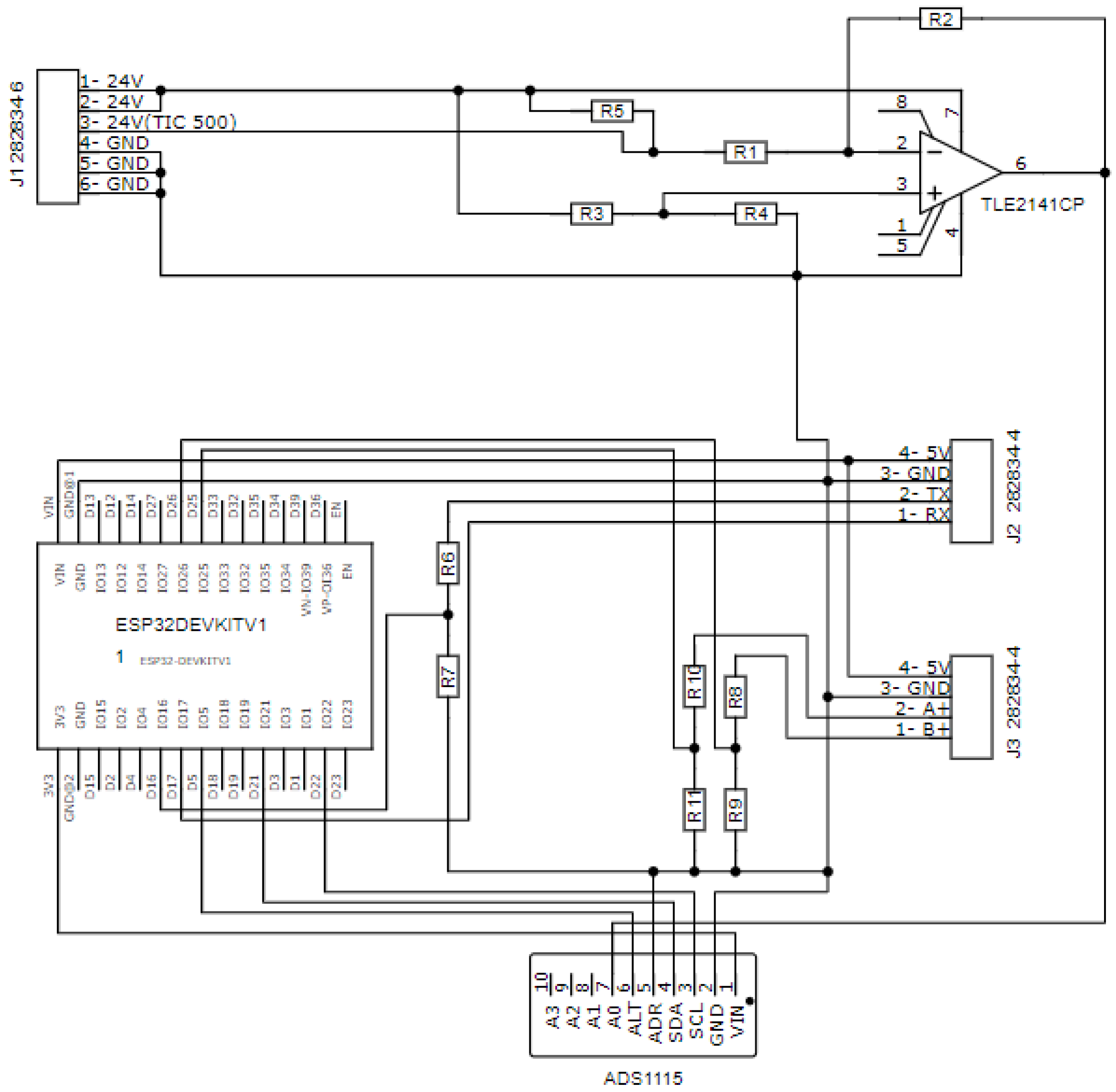
2.1.3. ESP32 Microcontroller and Communication Protocols

The ESP32 Microcontroller, is a series of low-cost, low-power SoC (System on Chip) microcontrollers designed and developed by the company, Espressif Systems. It is a feature-rich microcontroller with a variety of integrated peripherals for a wide range of applications. The ESP32 series employs two cores, 32-bit Tensilica Xtensa LX6 CPU, 448 KB ROM memory, 520 KB RAM memory, 4 MB flash memory, standard 802.11 b/g/n Wireless communication card, 2.4 GHz, built-in antenna on the board, STA/AP/STA+AP operation modes, Bluetooth BLE 4.2, and peripheral interface (GPIO, ADC, Hall sensor, DAC, UART, I2C, I2S, SPI, PWM); it can individually operate at a frequency of up to 240 MHz [39]. Due to compatibility and features, this microcontroller is featured in several projects. For example, Biswas and Iqbal [40] propose system monitoring for low-cost automated solar pumping for irrigation in developing countries, Bunkum et al. [41] proposed the development of a robotic arm for use in the operating room, which is controlled by joystick from anywhere, and Bolla et al. [42] proposed the implementation of a smart fuel station in the fueling process using Internet of Things (IoT) technology. Rai and Rehman [43] proposed a smart surveillance system, and Contardi et al. [44] proposed a biosensor coupled to ESP32-Webserver capabilities for continuous point-of-care oxygen saturation and heartrate monitoring.

A Universal Asynchronous Receiver Transmitter (UART) communication is a serial communication system, i.e., bit sequences. It uses only two signal lines (RX, TX) to complete full-duplex communication. To establish communication, a bit sequence consisting of start bit, data bit, parity bit and stop bit is required.

The ESP-NOW communication protocol [45] is a fast communication protocol that can be used to exchange small messages. It was developed by Espressif and allows multiple devices to communicate without using Wi-Fi. The protocol is similar to the low-power 2.4 GHz wireless connectivity that is usually deployed in wireless mice and has a transmission rate of 1 Mbps. ESP-NOW applies IEEE 802.11 technology, along with IE function developed by Espressif and encryption technology CCMP (Counter Mode with Cipher Block Chaining Message Authentication Code Protocol), to provide a secure, Wi-Fi-connectionless communication solution. The ESP-NOW protocol presents the following features: encrypted and unencrypted unicast communication, 250 bytes storage, and return function that can be set to inform the application layer about the success or failure of the transmission. It is unable to support Broadcast, but in station mode, it can support up to 10 devices in encrypted pairs and up to 20 unencrypted pairs, including encrypted pairs. To establish accurate communication, it is necessary to register both devices with the following data: media access control (MAC) address, channel number (0–15) and information on whether the data are encrypted or not. This communication protocol is very versatile and allows one-way or two-way communication in different configurations.

The I2C-Inter-Integrated Circuit is a communication protocol with a two-wire interface (SDA-serial data and SCL-serial clock) used to establish synchronous serial communication between a master and one or more slave devices. To establish this communication, the device generates the clock signal for the following bit sequences: one bit for communication start condition, seven address bits, one bit for read/write (R/W), two ACK/NACK bits-acknowledge/not acknowledge (0/1), and one bit for communication end. Normally, I2C allows communication between 128 devices (2ⁿ, n being the number of address bits). The addresses (0 to 127) should never be duplicated, and the devices operate at a normal frequency of 100 kbit/s. The above-mentioned communication protocols were used in this study for the following purpose:

• UART—used to establish communication between ESP32 of each axis of the robot with its respective stepper motor controller and establish communication between main ESP32 and PC (MATLAB interface) through USB to TTL converter.
• ESP NOW—used to establish communication between the main ESP32 with the ESP32s of each axis.
• I2C—used to establish communication between the ESP32 of each axis with the ADC-analog–digital converter to monitor the consumption (electrical current) of each stepper motor.

2.2. Software

This section presents some of the main software, such as SolidWorks [46], that enabled the design, drawing and visualization of the 3D parts for the construction of the robotic arm structure, the Arduino’s Integrated Development Environment (IDE) [47] for programming and compiling the code for the ESP32 microcontroller in C/C++ language and the MATLAB [48] software to develop the user guide for the interface between the user and the robotic arm.

2.3. Methods and Algorithms

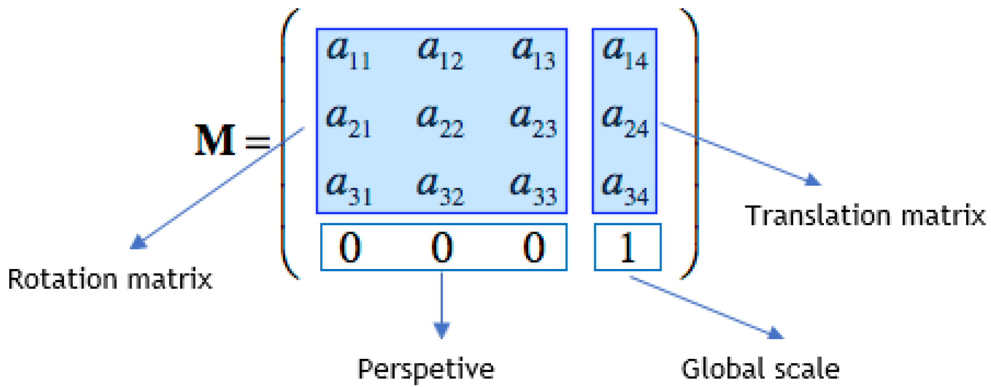
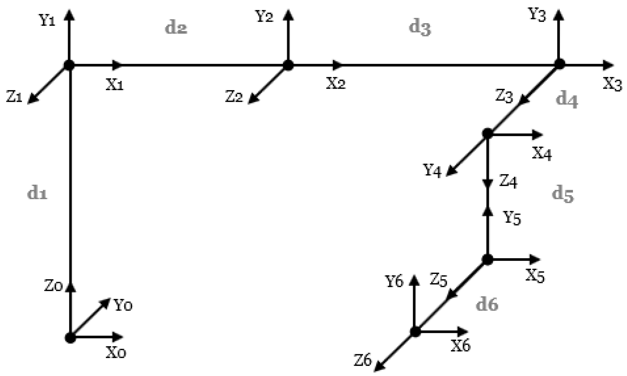
2.3.1. Homogeneous Transformation Matrix

The homogeneous transformation matrix [49] is used to represent the orientation and position of a coordinate system within a “world” coordinate system. Sub-transformations, such as rotation matrix, translation, perspective, and global scale, are appropriately combined into a single three-dimensional homogeneous transformation matrix. Figure 3 shows the homogeneous transformation matrix and its sub-transformations.

2.3.2. Direct Kinematics

Direct kinematics allows the position and orientation of the tool structure to be determined given all its manipulator joint parameters and the respective joint angle and distance. A convention commonly used to calculate the parameters required in the kinematic model in robotics applications is the Denavit–Hartenberg (DH) convention, which has four parameters [50] associated with the link and joint:

• a_i: link length;
• α_i: link torsion;
• d_i: offset;
• θ_i: joint angle.

This convention gives rise to an individual homogeneous transformation matrix as the product of four basic transformations [51], as presented in Equations (1) and (2):

$${\mathrm{A}}_{\mathrm{i}}={\mathrm{Rot}}_{\mathrm{Z},{\mathsf{\theta }}_{\mathrm{i}}}·{\mathrm{Trans}}_{\mathrm{Z},{\mathrm{d}}_{\mathrm{i}}}·{\mathrm{Trans}}_{\mathrm{X},{\mathrm{a}}_{\mathrm{i}}}·{\mathrm{Rot}}_{\mathrm{X},{\mathsf{\alpha }}_{\mathrm{i}}},$$

(1)

Performing the multiplications of the matrices, the DH matrix is obtained [51]:

$${\mathrm{A}}_{\mathrm{i}}=\left[\begin{array}{cccc}{\mathrm{C}}_{{\mathsf{\theta }}_{\mathrm{i}}}& -{\mathrm{S}}_{{\mathsf{\theta }}_{\mathrm{i}}}·{\mathrm{C}}_{{\mathsf{\alpha }}_{\mathrm{i}}}& {\mathrm{S}}_{{\mathsf{\theta }}_{\mathrm{i}}}·{\mathrm{S}}_{{\mathsf{\alpha }}_{\mathrm{i}}}& {\mathrm{a}}_{\mathrm{i}}·{\mathrm{C}}_{{\mathsf{\theta }}_{\mathrm{i}}}\\ {\mathrm{S}}_{{\mathsf{\theta }}_{\mathrm{i}}}& {\mathrm{C}}_{{\mathsf{\theta }}_{\mathrm{i}}}·{\mathrm{C}}_{{\mathsf{\alpha }}_{\mathrm{i}}}& -{\mathrm{C}}_{{\mathsf{\theta }}_{\mathrm{i}}}·{\mathrm{S}}_{{\mathsf{\alpha }}_{\mathrm{i}}}& {\mathrm{a}}_{\mathrm{i}}·{\mathrm{S}}_{{\mathsf{\theta }}_{\mathrm{i}}}\\ 0& {\mathrm{S}}_{{\mathsf{\alpha }}_{\mathrm{i}}}& {\mathrm{C}}_{{\mathsf{\alpha }}_{\mathrm{i}}}& {\mathrm{d}}_{\mathrm{i}}\\ 0& 0& 0& 1\end{array}\right],$$

(2)

Equations (1) and (2) refer to the position and orientation of the link in the space, where A_i is the transformation matrix, S is sine, C is cosine and i is the number of degrees of freedom. For i degrees of freedom, the position and orientation of the tool structure relative to the inertial structure (fixed referential) are given by a homogeneous transformation matrix [50] represented in Equation (3):

$$\mathrm{A}=\left[\begin{array}{cc}{\mathrm{R}}_{\mathrm{i}}^0& {\mathrm{O}}_{\mathrm{i}}^0\\ 0& 1\end{array}\right]={ \mathrm{T}}_{\mathrm{i}}^0\left({\mathrm{q}}_1,\dots {\mathrm{q}}_{\mathrm{i}}\right)={\mathrm{A}}_1\left({\mathrm{q}}_1\right)·{\mathrm{A}}_2\left({\mathrm{q}}_2\right)·{\mathrm{A}}_3\left({\mathrm{q}}_3\right)\dots { \mathrm{A}}_{\mathrm{i}}\left({\mathrm{q}}_{\mathrm{i}}\right),$$

(3)

where A is the homogeneous matrix (position and orientation of the effector in relation to the base), R is the rotation matrix, q is the angle or displacement associated with the joint, and O is the translation matrix.

The homogeneous transformation can be represented using the 4 DH parameters. To achieve this, it is necessary to define and establish rules for some references presented in the conditions given by Equations (4) and (5) [51]:

$${\hat{\mathrm{X}}}_{\mathrm{i}+1} ⟂{\mathrm{Ẑ}}_{\mathrm{I}},$$

(4)

$${\hat{\mathrm{X}}}_{\mathrm{i}+1}{\displaystyle \bigcap }{\mathrm{Ẑ}}_{\mathrm{I}} \mathrm{para} \mathrm{i}>0,$$

(5)

Equations (4) and (5) are rules to determine the kinematics of the manipulator.

2.3.3. Inverse Kinematics

Inverse kinematics is a subdomain of kinematics, and it calculates the required positions of joints to achieve a desired position and orientation [50]. Inverse kinematics is a complex and unpredictable problem relative to direct kinematics:

• There may be multiple, or even infinite, solutions;
• There may be no solution (the generalized position is outside the workspace);
• They are non-linear equations, so an analytical solution is not always possible.

In general, inverse kinematics requires large calculations, using analytical or iterative numerical methods. The analytical method is applied when the problem is simple and allows all the solutions to be obtained; otherwise, iterative number methods are used (several iterations to try to converge to the solution with a given error). The application of inverse kinematics, the values of the joint parameters that will place the tool structure in the desired position and orientation (within the working area), and a homogeneous matrix H with the desired positions and orientations are provided by Equation (6) [51].

$$\mathrm{H}=\left[\begin{array}{cc}\mathrm{R}& \mathrm{O}\\ 0& 1\end{array}\right],$$

(6)

for a given robotic manipulator with n degrees of freedom, applying the DH convention, Equation (7) is given by [51]:

$${\mathrm{T}}_{\mathrm{n}}^0\left({\mathrm{q}}_1,\dots {\mathrm{q}}_{\mathrm{n}}\right)={\mathrm{A}}_1\left({\mathrm{q}}_1\right)·{\mathrm{A}}_2\left({\mathrm{q}}_2\right)·{\mathrm{A}}_3\left({\mathrm{q}}_3\right)\dots { \mathrm{A}}_{\mathrm{n}}\left({\mathrm{q}}_{\mathrm{n}}\right),$$

(7)

finding the solution (angle of each joint) to satisfy Equation (8) is given by [50]:

$${\mathrm{T}}_{\mathrm{n}}^0\left({\mathrm{q}}_1,\dots {\mathrm{q}}_{\mathrm{n}}\right)=\mathrm{H} ,$$

(8)

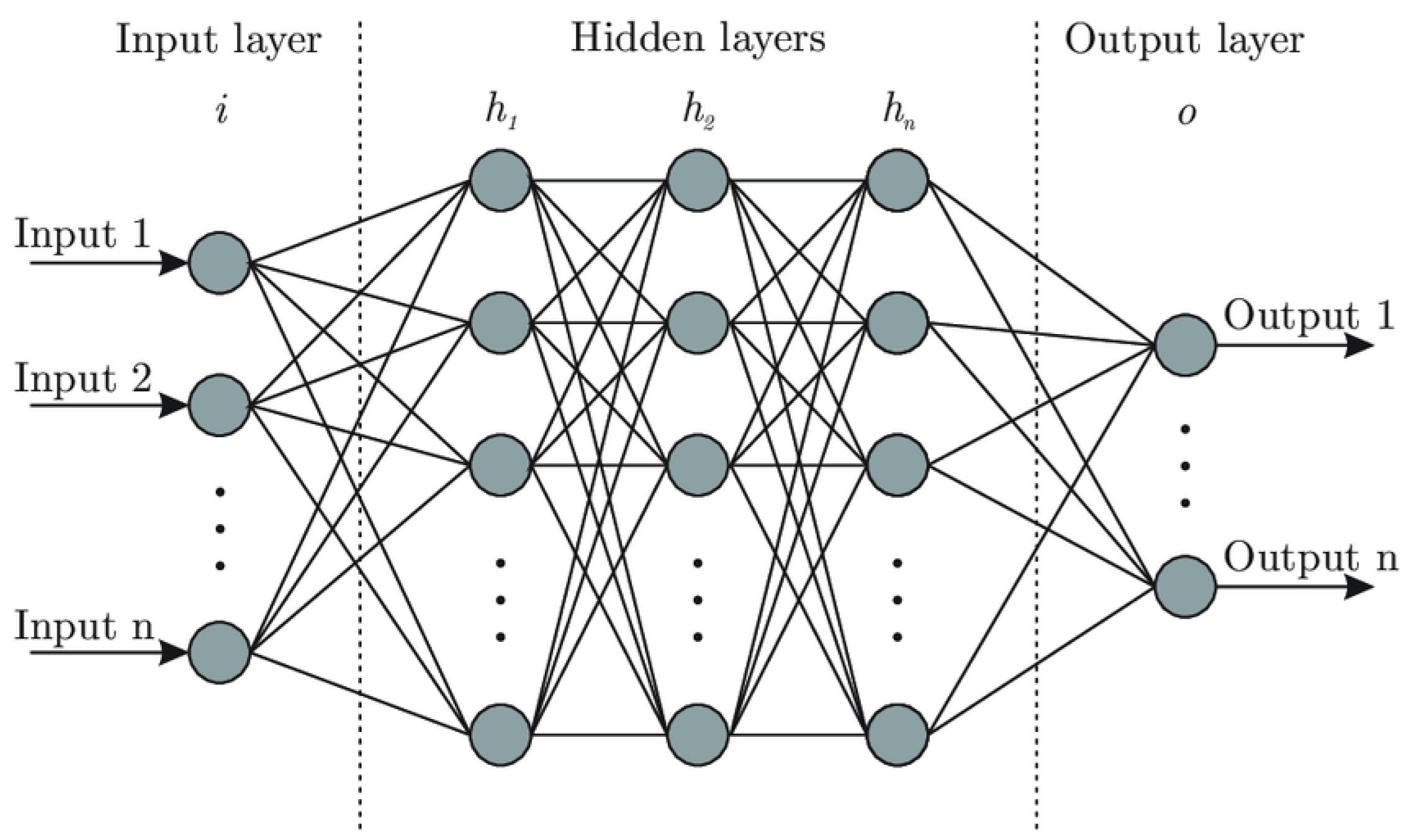
2.3.4. ANN—Artificial Neural Network

An artificial neuronal network is a computationally implemented algorithm based on the functioning of the human brain [52]. It is composed of neurons or nodes, interconnected so that the output of a neuron can be used as an input for others. The function of the network is determined by the connection between neurons, usually organized into groups called layers (input, output and hidden). Figure 4 represents the architecture of an artificial neural network, where the input layer represents the medium in which data are presented to the network, the output layer shows the response of the network to a given input, and the hidden layer usually consists of many neurons linked together to interleave an output.

Many values in different areas of engineering, as well as aiding the resolution and optimization of everyday problems have been shown by the development and application of computational mathematical such as Monte Carlo simulation technique [53]; meta-heuristics such as genetic algorithms [54,55], ant colony [56], and particle swarm optimization [57]; fuzzy logic [58]; and artificial intelligence algorithms that can based in machine learning techniques such as artificial neural network [59], or deep learning algorithms [60,61].

An artificial neural network is used as a predictive means of detecting a possible collision by increasing the electric current. The network is trained based on the type of movement, position, and orientation to reach the correct speed and payload, while always monitoring the state of the electric current.

3. Results

In this chapter, the parts, assembly processes and final structures of the robotic arm are presented. Additionally, the mathematical calculations of the DH convention, electrical/electronic circuit sizing, and user interface with the final robotic manipulator are presented.

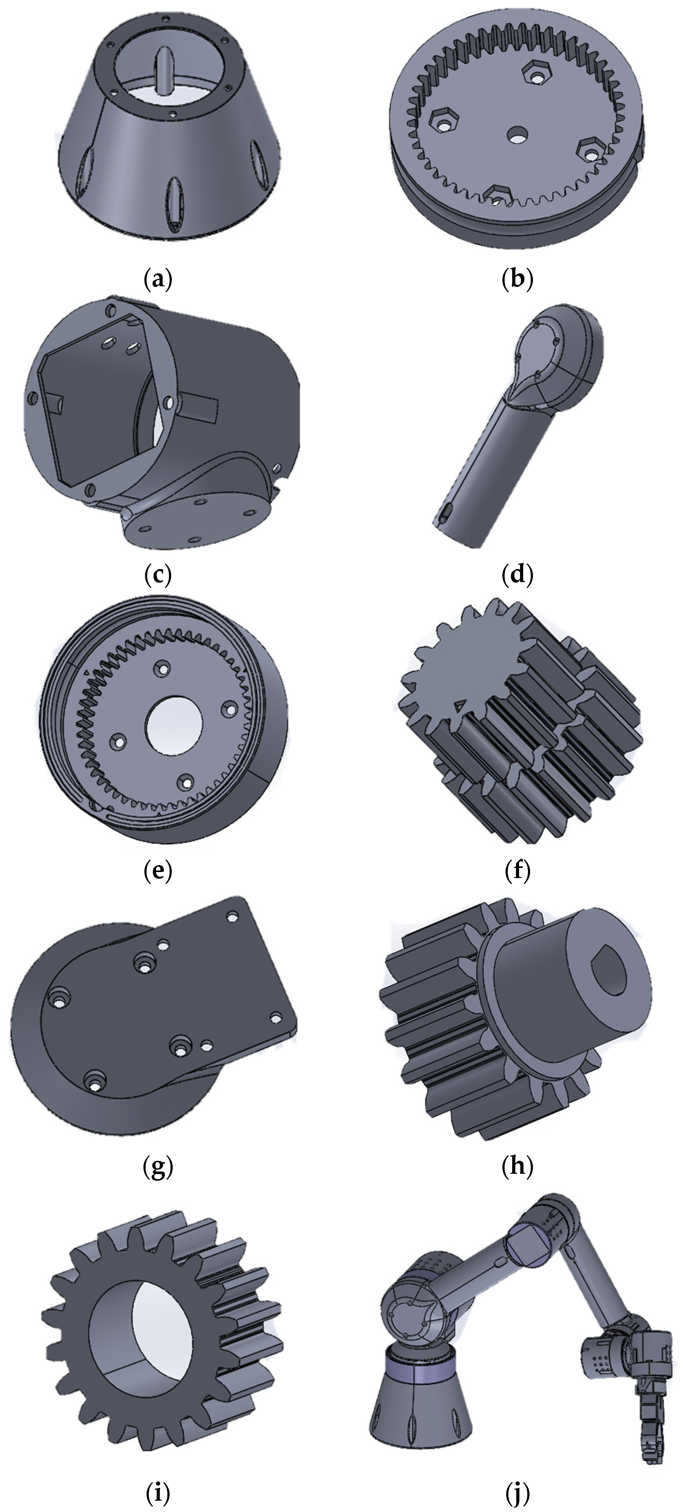
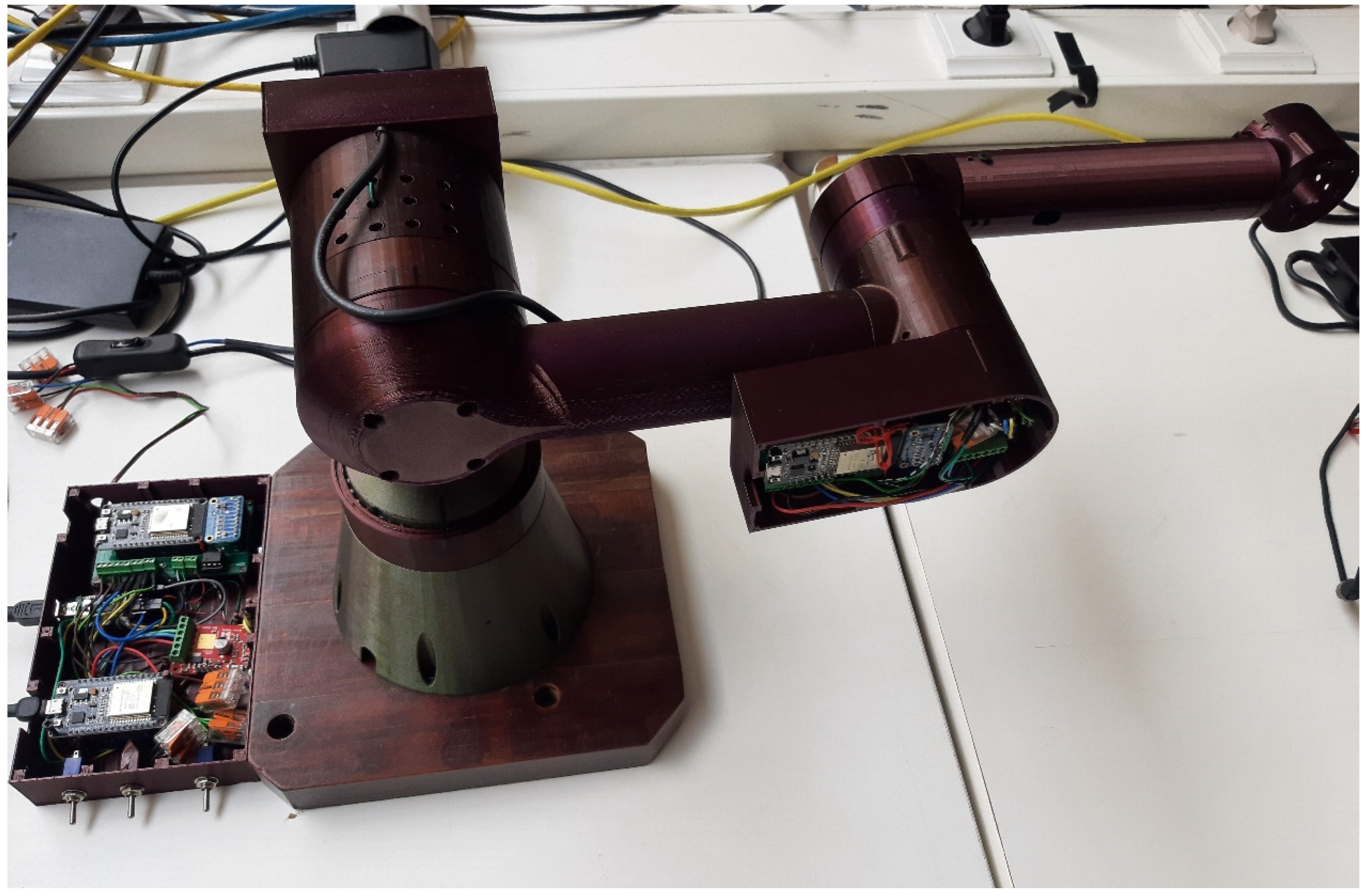
3.1. Parts and Structure of the Robotic Arm

Figure 5 shows the final 3D parts and structure of the robotic arm designed and modified in SolidWorks software and based on the WE-R2.4 robot model [15].

3.2. Mathematical Formulation of the Convention—DH and Direct/Inverse Kinematics

The kinematics of the manipulator is determined by establishing the rules for references by applying Equation (4) to Equation (5). Figure 6 presents the kinematics of the manipulator.

Table 1. Distance values between links.

d	Distance [mm]
d1	163.00
d2	204.00
d3	230.00
d4	100.00
d5	100.00
d6	100.00

includes the values of the distances between the links.

Subsequently, the DH parameters presented in

Table 2. DH parameters.

Link	a [mm]	α [°]	d [mm]	θ [°]
L01	0	90	d1	θ1
L12	d2	0	0	θ2
L23	d3	0	0	θ3
L34	0	90	d4	θ4
L45	0	−90	d5	θ5
L56	0	0	d6	θ6

.

Applying Equation (2) and with DH parameters from Table 2, we obtain the individual homogeneous transformation matrix (A1, A2, A3, A4, A5, A6), and by denoting C as cosine and S as sine we obtain:

$$\mathrm{A}1=\left[\begin{array}{cccc}\mathrm{C}\mathsf{\theta }1& 0& \mathrm{S}\mathsf{\theta }1& 0\\ \mathrm{S}\mathsf{\theta }1& 0& -\mathrm{C}\mathsf{\theta }1& 0\\ 0& 1& 0& \mathrm{d}1\\ 0& 0& 0& 1\end{array}\right],$$

(9)

$$\mathrm{A}2=\left[\begin{array}{cccc}\mathrm{C}\mathsf{\theta }2& -\mathrm{S}\mathsf{\theta }2& 0& \mathrm{d}2·\mathrm{C}\mathsf{\theta }2\\ \mathrm{S}\mathsf{\theta }2& \mathrm{C}\mathsf{\theta }2& 0& \mathrm{d}2·\mathrm{S}\mathsf{\theta }2\\ 0& 0& 1& 0\\ 0& 0& 0& 1\end{array}\right],$$

(10)

$$\mathrm{A}3=\left[\begin{array}{cccc}\mathrm{C}\mathsf{\theta }3& -\mathrm{S}\mathsf{\theta }3& 0& \mathrm{d}3·\mathrm{C}\mathsf{\theta }3\\ \mathrm{S}\mathsf{\theta }3& \mathrm{C}\mathsf{\theta }3& 0& \mathrm{d}3·\mathrm{S}\mathsf{\theta }3\\ 0& 0& 1& 0\\ 0& 0& 0& 1\end{array}\right],$$

(11)

$$\mathrm{A}4=\left[\begin{array}{cccc}\mathrm{C}\mathsf{\theta }4& 0& \mathrm{S}\mathsf{\theta }4& 0\\ \mathrm{S}\mathsf{\theta }4& 0& -\mathrm{C}\mathsf{\theta }4& 0\\ 0& 1& 0& \mathrm{d}4\\ 0& 0& 0& 1\end{array}\right],$$

(12)

$$\mathrm{A}5=\left[\begin{array}{cccc}\mathrm{C}\mathsf{\theta }5& 0& -\mathrm{S}\mathsf{\theta }5& 0\\ \mathrm{S}\mathsf{\theta }5& 0& \mathrm{C}\mathsf{\theta }5& 0\\ 0& -1& 0& \mathrm{d}5\\ 0& 0& 0& 1\end{array}\right],$$

(13)

$$\mathrm{A}6=\left[\begin{array}{cccc}\mathrm{C}\mathsf{\theta }6& -\mathrm{S}\mathsf{\theta }6& 0& 0\\ \mathrm{S}\mathsf{\theta }6& \mathrm{C}\mathsf{\theta }6& 0& 0\\ 0& 0& 1& \mathrm{d}6\\ 0& 0& 0& 1\end{array}\right],$$

(14)

The final homogeneous matrix to which the position and orientation of the effector is related is caused by the successive multiplication of Equations (9)–(14).

Inverse kinematics is an important and challenging problem in the field of robotics. The analytical solution to the problem is complex and time-consuming depending on the manipulator configuration and the number of solutions. An iterative numerical method was applied to solve the inverse kinematics problem using a particle swarm optimization (PSO) algorithm. Alkayyali and Tutunji [62] applied PSO and obtained good results compared to other meta heuristic studies in the literature. The proposed algorithm generates solutions for inverse kinematics through a space search, i.e., it finds the ideal values of the six joint angles to minimize the error. Figure 7 shows the pseudocode of the PSO algorithm used in the inverse kinematics process.

The pseudo code of the PSO in Figure 7 aims to minimize errors. Essentially, the algorithm searches for the angles of each joint by means of particle velocity, applies direct kinematics (calculates the position and orientation), and then calculates the error between the intended position and the position with the searched solution. The speed of the particle decreases as the error decreases. The algorithm is in a cycle until it reaches the stopping criterion (error smaller than the desired error: if it has not reached the maximum number of iterations or if it has not reached the maximum iterative time).

Equations:

$$\mathrm{Xi}=\mathrm{L}\_\inf +\left(\mathrm{L}\_\sup -\mathrm{L}\_\inf \right)·\mathrm{r}$$

(15)

$$\mathrm{Error}=\mathsf{\rho }·\mathrm{Ep}+\left(1-\mathsf{\rho }\right)·\mathrm{Er}$$

(16)

$$\mathrm{Vi}\left(\mathrm{iter}\right)=\mathrm{K}\left[\mathrm{W}·\mathrm{Vi}\left(\mathrm{iter}-1\right)+ \mathrm{c}1·\mathrm{r}1·\left(\mathrm{xPbest}- \mathrm{Xi}\left(\mathrm{iter}-1\right)\right)+ \mathrm{c}2·\mathrm{r}2·\left(\mathrm{xbest}- \mathrm{Xi}\left(\mathrm{iter}-1\right)\right)\right]$$

(17)

$$\mathrm{Xi}\left(\mathrm{iter}\right)=\mathrm{Xi}\left(\mathrm{iter}-1\right)+ \mathrm{Vi}\left(\mathrm{iter}\right)$$

(18)

$$\mathrm{Ep}=\frac{{\left|\left|{\mathrm{P}}_{\mathrm{PSO}}-{\mathrm{P}}_{\mathrm{d}}\right|\right|}^2}{{\left|\left|{\mathrm{P}}_{\mathrm{d}}\right|\right|}^2}$$

(19)

$$\mathrm{Er}=\frac{{\left|\left|{\mathrm{R}}_{\mathrm{PSO}}-{\mathrm{R}}_{\mathrm{d}}\right|\right|}^2}{{\left|\left|{\mathrm{R}}_{\mathrm{d}}\right|\right|}^2}$$

(20)

$$\mathsf{\rho }=0.7·{\mathrm{e}}^{-\mathrm{Er}}+0.3$$

(21)

$$\mathrm{K}=\frac{2·\mathrm{r}}{\left|2-\mathsf{\phi }-\sqrt{{\mathsf{\phi }}^2-4·\mathsf{\phi }}\right|},$$

(22)

$$\mathsf{\phi }= \mathrm{c}1·\mathrm{r}1+ \mathrm{c}2·\mathrm{r}2,$$

(23)

$$\mathrm{W}={ \mathrm{W}}_{\max }-\frac{{\mathrm{W}}_{\max }-{ \mathrm{W}}_{\min }}{\mathrm{itermax}}·\mathrm{iter}$$

(24)

where:

Xi is the random initial position of the particles within a given boundary;

(L_sup and L_inf) error is the error between the calculated position/orientation and the intended position/orientation;

Vi is particle speed;

Ermin is the minimum desired error and represents 1% initial error [62];

t/t_max are the instantaneous/maximum iterative time;

iter/itermax are the instantaneous/maximum iteration;

Gbest/xGbest are the global error/current best solution;

Pbest/xPbest are the population error/current solution of population;

L_inf/L_sup are the lower/upper limits in degrees of each axis;

Ppso/Rpso are the position/rotation calculated by PSO;

P_d/R_d are the desired position/orientation;

W is the inertia factor;

r, r1, and r2 are random numbers between (0,1);

c1 and c2 are social and cognitive factors;

k is the constriction coefficient;

φ and p are constants;

d is the problem dimension (six axes);

N is the population.

According to [52], N belongs to (0,1000)and itermax 1000. To reduce the convergence time, t_max = 10 [s].

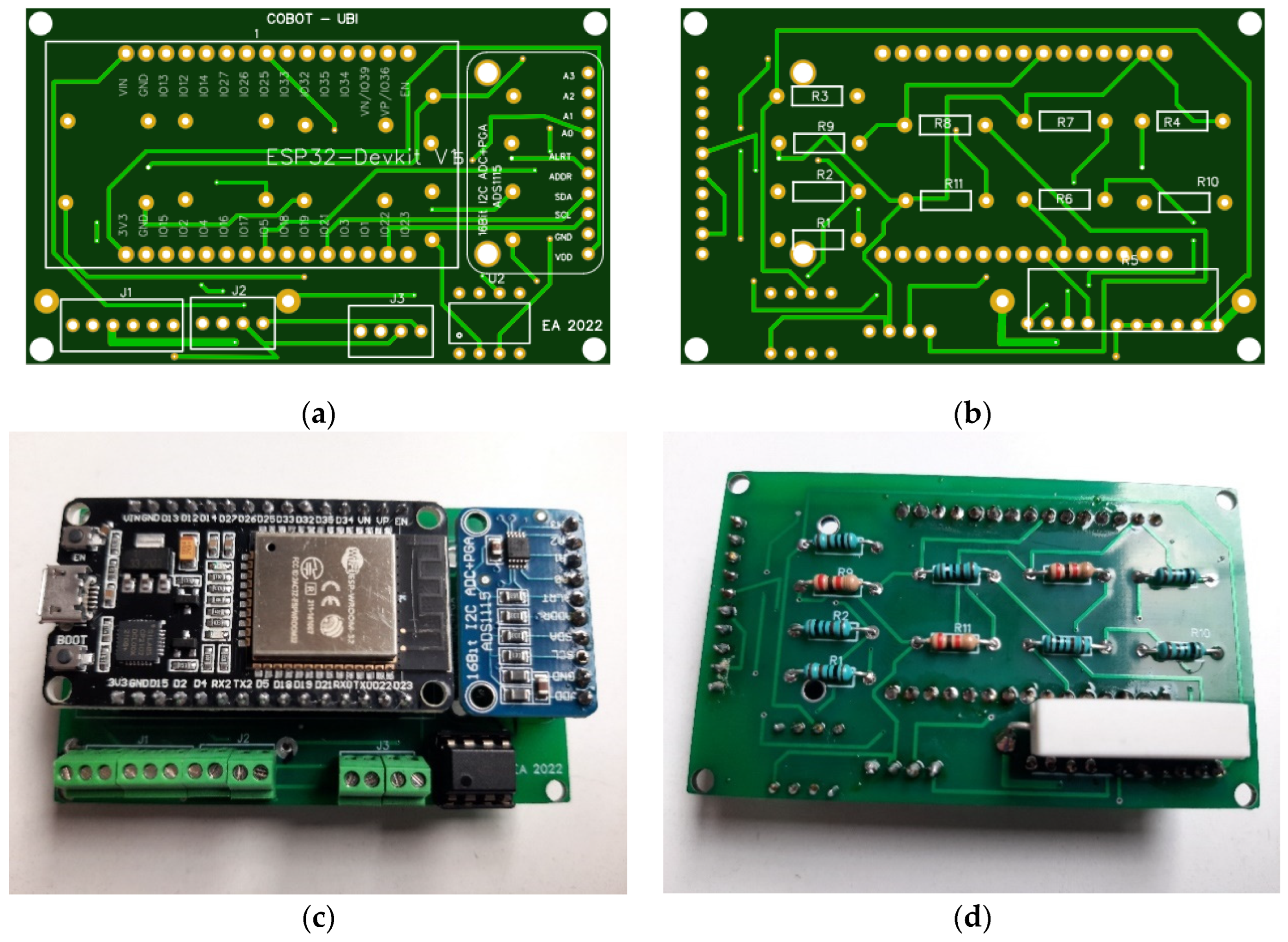
3.3. Electrical Circuit and Control

In robotics, it is very difficult to reduce the wiring on a robot arm to provide it with more mobility. On the other hand, information processing requires reduced time to provide a quick response. By the specifications of the ESP microcontroller, information processing presents robust characteristics in terms of processing, reliability, and communication protocol; therefore, a main ESP32 is used, which establishes PC (User Interface—MatLab) UART communication via a USB to TTL converter. The main ESP32 also establishes wireless communication using the ESP NOW protocol between the six ESPs on each axis of the robotic arm. Figure 8 shows the connection scheme between ESP32 and PC.

Figure 9 shows the electrical connection between the ESP32 of each axis, encoder, analogue–digital converter (ADS1115), operational amplifier and the stepper motor drive (TIC 500).

The connections are established through the terminal designated as “J1, J2 and J3”. The J1 terminal with six terminals receives the power supply for the PCB of the respective axis, the motor drive (TIC 500) and has the power supply for the next axis. The four-terminal J2 terminal establishes the electrical connection (5V for ESP32 and encoder) and UART communication between the ESP32 of the current axis and the motor drive circuit (TIC 500). Finally, terminal J3, also four-terminal, establishes the electrical connection (5V) and signals (A+ and B+) from the encoder and the ESP32. To interconnect the circuit components of Figure 9 and minimize the area, a printed circuit board (PCB) was developed and printed, as shown in Figure 10.

For the control and positioning of a certain desired angle with the stepper motor, a control via a ramp with different speed levels (number of pulses) is applied to the motor. The number of pulses to be applied to the stepper motor depends on some parameters such as error in degrees and the desired speed. Figure 11 plots the number of pulses ramp applied as a function of the desired parameters. The control ramp is used because the action and reaction time is not immediate, i.e., the motor never stops at the desired position. Once in motion, the motor does not immediately stop due to the inertia caused by the angular velocity. The inertia tends to be greater, the higher the speed. This technique serves to minimize the error in positioning the motor by adjusting the parameters to do so.

Its parameters are:

A—Default minimum error [°];

B—Minimum error for constant minimum speed [°];

C—Maximum error before approach [°];

D—Minimum approach speed pre-set [PPS];

E—Maximum approach speed pre-set [PPS];

F—Speed of movement away from approach [PPS];

K—Maximum error [°].

Equations of the tangent line:

$$\mathrm{K}=2^{\mathrm{T}}, \mathrm{T} \mathrm{is} \mathrm{type} \mathrm{of} \mathrm{error} \left(1-\mathrm{simple} \mathrm{error}, 2-\mathrm{quadratic} \mathrm{error}\right)$$

(25)

$$\mathrm{C}={\left(1+ \% \mathrm{normal} \mathrm{velocity}\right)}^{\mathrm{T}}$$

(26)

$$\mathrm{m}=\frac{\mathrm{E}-\mathrm{D}}{\mathrm{K}-\mathrm{B}}$$

(27)

$$\mathrm{E}-\mathrm{D} =\mathrm{m} ·\left(\mathrm{K}-\mathrm{B}\right)$$

(28)

$$\mathrm{E}-\mathrm{D} =\frac{\mathrm{E}-\mathrm{D}}{\mathrm{K}-\mathrm{B}} ·\left(\mathrm{K}-\mathrm{B}\right)$$

(29)

$$\mathrm{Y}=\mathrm{m}·\mathrm{x}+\mathrm{b}=\frac{\mathrm{E}-\mathrm{D}}{\mathrm{K}-\mathrm{B}} ·\mathrm{Erro}-\mathrm{B}·\frac{\mathrm{E}-\mathrm{D}}{\mathrm{K}-\mathrm{B}}+\mathrm{D}$$

(30)

Y is the number of pulses applied to the motor and is given in Equation (31) as:

$$\mathrm{Y}=\{\begin{array}{c}\mathrm{F}, \mathrm{if} \mathrm{error}>\mathrm{C} \\ \frac{\mathrm{E}-\mathrm{D}}{\mathrm{K}-\mathrm{B}} ·\mathrm{Erro}-\mathrm{B}·\frac{\mathrm{E}-\mathrm{D}}{\mathrm{K}-\mathrm{B}}+\mathrm{D}, \mathrm{if} \mathrm{error}\le \mathrm{C} \end{array},$$

(31)

Converting pulses into degrees

To calculate the position in degrees by number of encoder pulses, the encoder resolution [PPR] was programmed to 2500 pulses per revolution. The gear system, called planetary, consists of a sun pinion (Figure 5h), planetary (Figure 5f) and crown (Figure 5b). The pinion (P) has 15 teeth, the planetary at the bottom (Pi) has 18 teeth, and at the top, (Ps) has 15 teeth and crown (C) has 48 teeth. The planetary case ratio (PCR) is calculated in Equation (32) as:

$$\mathrm{PCR} =\frac{\mathrm{P}}{\mathrm{Pi}}·\frac{\mathrm{Pi}}{\mathrm{Ps}}·\frac{\mathrm{Ps}}{\mathrm{C}}=\frac{15}{18}·\frac{18}{15}·\frac{15}{48}=0.3125$$

(32)

The result of Equation (32) represents the turn in degrees of the link when the stepper motor shaft makes a full turn, i.e., when the motor makes a full turn (360°), the arm link makes a 0.3125 turn (112.50°). The angle per full pulse of the encoder relative to the motor shaft RRMS (resolution relative to the motor shaft) is calculated in Equation (33) as:

$$\mathrm{RRMS} =\frac{360}{2·\mathrm{PPR}}=\frac{360}{2·2500}=0.0720°$$

(33)

The angle per full pulse of the encoder relative to the RRRA arm link (resolution relative to the robotic arm link) is calculated in Equation (34) as:

$$\mathrm{RRRA} =\mathrm{RRMS}·\mathrm{PCR}=0.0720 ·0.3125=0.0225°$$

(34)

3.4. Graphical User Interface—MATLAB

To establish communication between the human and the robotic arm, a graphical user interface (GUIDE—Graphical User Interface Development Environment) was developed in MATLAB with several menus (connect menu, alarm, control, and program), and it became possible to establish communication, view or change parameters, and move the robotic arm.

The “Connect” menu, as shown in Figure 12, allows communication to be established with the robotic arm. This window allows you to view and change the inverse kinematics parameters, link lengths, movement limit of each axis and collision distances. It also allows commands to be sent and received.

The right side of Figure 12, designated as a command stand, appears in all menus, and it is possible to signal alarm, communication, and drive status. It also allows the execution mode (manual, automatic or test) to be selected, as well as enabling, disabling, and resetting robot defects and sending some predefined commands.

Figure 13 shows the “Mover” menu. In this menu, it is possible to view the position in degrees of each joint, position, and orientation of the tool, make the movement of each joint, move/orient the tool, and change the speed percentage of movement. It is also possible to change the incremental value of the speed percentage, joint angle, and tool distance. Finally, the robot arm can be moved to the calibration position (reference home position).

Additionally, an “Alarm” menu was developed to view the active alarm(s) and the history of the alarms. These alarms are notified with the date and time of occurrence and their description.

A “Control” menu, as shown in Figure 14, is used to view some data such as the voltage applied to the motor driver, the current consumed and the encoder pulse(s). It is possible to view and change the driver status, calibrate the axes, reset the ESP32s, and change the type of step in order to move, change and view the control parameters.

For the robot to execute a sequence of movements (points), a last menu was created called “Program”, where it is possible to create, modify, execute, and delete points. This window can include a sequence of movements and save them, so that the robot repeats that sequence for the programmed number of times, or indefinitely.

3.5. 3D Printing and Assembly of the Robotic Arm

After developing the 3D design parts in SolidWorks software, they were saved in “stl” extension (stereolithography file) and then converted to Gcode extension (G code), recognizable in the 3D printer. The parts were printed by a 3D printer (Artillery Sidewinder ×1), mostly with PLA to print the parts (except the coupling pinion on the motor shaft) and structure of the robotic arm and PETG to print the coupling pinion to a motor shaft filament. PLA was used since its characteristics allow for printing with fine details and easy printing. This method achieved good results in the literature and PETG due to its high deformation temperature characteristics since the stepper motor heats up and the pinion is attached to the shaft.

Table 3. Main print parameters for different filaments.

Filament	Temperature [°C]		Print Speed [mm/s]	Layer Height [mm]	Infill Density [%]
	Print	Bed
PLA	215	70	80	0.2	20–50
PETG	240	80	80	0.2	40

shows the optimal configurable parameters for different filament types for the printing process, and Figure 15 shows the final assembly of the developed robotic arm.

4. Analysis and Discussion of Results

This chapter presents the results of the tests performed on the developed collaborative robot. The tests performed were related to payload and positioning accuracy.

During assembly, when performing test no. 1, it was not possible to fully assemble the manipulator due to the weight, and the tests were only performed with the first three axes, with 10% or 30% of speed and both at 1/8 of step.

4.1. Test No. 1: Payload

Test no. 1 was performed to determine the payload, i.e., the maximum weight that the robotic manipulator can support both when stationary and when moving. When the motors of the manipulator are not driven, the load is supported by the torque created in the gearbox. When in motion, it is ensured by the torque produced by the motor(s). To perform this test, we resorted to the physical consideration that the force is maximum for a given weight and the horizontal distance (0°) of the mass to the center of movement is greater. The robotic arm was extended horizontally, which corresponds to zero degrees (0°) for axes two and three, and weight was gradually added in the center of the final effector until the arm began to sag. Subsequently, the masses were weighed, obtaining a maximum weight of 314 g. The results of test no. 1 (payload) determine the maximum weight that the robotic arm supports while stationary or moving and with or without the arm fully extended. The developed robot supports 0.314 kg. This result is quite acceptable, since the developed arm is entirely made of PLA, including the pinion and gear set, motor without mechanical lock, and low electromechanical torque.

4.2. Test No. 2: Positioning Error

Test no. 2 was used to evaluate the positioning accuracy and assess the method and strategy of Figure 11; therefore, it required five positions to be selected. The robot was automatically positioned at 35% speed and with the payload attached. The variations in the positions were recorded before and after disabling the motor driver.

Table 4. Root mean square error (RMSE) associated with test no. 2.

	Position Still with Active Drive					Position after Disabled Drive
	P1	P2	P3	P4	P5	P1	P2	P3	P4	P5
Joints [°]	3.51 × 10−2	1.41 × 10−2	1.29 × 10−2	8.16 × 10−3	1.41 × 10−2	4.08 × 10−2	7.79 × 10−2	5.35 × 10−2	1.83 × 10−2	4.93 × 10−2
Position [mm]	1.42 × 10−1	9.99 × 10−2	8.80 × 10−2	1.78 × 10−2	7.25 × 10−2	1.65 × 10−1	6.27 × 10−1	1.71 × 10−1	8.44 × 10−2	1.06
Orientation [°]	3.51 × 10−2	1.73 × 10−2	1.73 × 10−2	0.00	1.83 × 10−2	4.04 × 10−2	1.10 × 10−1	8.16 × 10−3	2.31 × 10−2	2.54 × 10−1

presents the mean square error influenced by test no. 2 in relation to the five selected positions.

The results obtained in test no. 2, for which the errors are shown in Table 4, present a relatively low and acceptable error, being the result of pinion and toothed ring wear, errors in measurement and conversion, action and response time to the motor, and the inertia caused by the weight of the payload and the robotic arm.

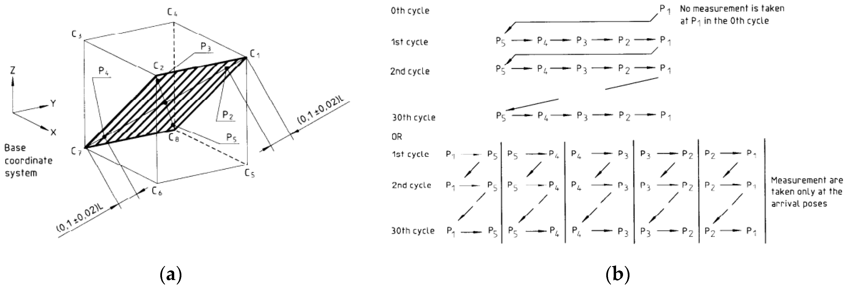
4.3. Test No. 3: Accuracy and Repeatability

Test no. 3 was used to evaluate the accuracy and repeatability according to ISO 9283 [63]. The test results for thirty repetitive movements going through a sequence of five positions are shown in Figure 16. This test was conducted with the maximum payload, an environmental temperature of 20 °C, and at 10% and 35% of the nominal speed. Upon reaching each position, the angles of each joint, position and orientation of the effector are recorded.

Table 5. Standard deviation of joint angle, position, and orientation.

	Joint			Position			Orientation
	θ1 [°]	θ2 [°]	θ3 [°]	X [mm]	Y [mm]	Z [mm]	X [°]	Y [°]	Z [°]
P1	0.005	0.002	0.018	0.025	0.044	0.063	0.00	0.00	0.02
P2	0.004	0.004	0.018	0.031	0.013	0.068	0.00	0.00	0.02
P3	0.005	0.009	0.013	0.031	0.018	0.085	0.00	0.00	0.02
P4	0.000	0.002	0.021	0.034	0.031	0.069	0.00	0.00	0.02
P5	0.004	0.003	0.018	0.026	0.052	0.050	0.00	0.00	0.02

represents the deviation of joint angle, position, and orientation from the desired position during the test.

With the data recorded during the test, we calculated the following [53]:

Position accuracy (APp) as:

$$\mathrm{APp}=\sqrt{{\left(\overline{\mathrm{x}}-{\mathrm{x}}_{\mathrm{c}}\right)}^2+{\left(\overline{\mathrm{y}}-{\mathrm{y}}_{\mathrm{c}}\right)}^2+{\left(\overline{\mathrm{z}}-{\mathrm{z}}_{\mathrm{c}}\right)}^2},$$

(35)

where $\overline{\mathrm{x}}$, $\overline{\mathrm{y}}$ e $\overline{\mathrm{z}}$ are the averages of the positions obtained and ${\mathrm{x}}_{\mathrm{c}}$, ${\mathrm{y}}_{\mathrm{c}}$ e ${\mathrm{z}}_{\mathrm{c}}$ are the positions commanded.

The positioning repeatability (RPι) is calculated as:

$${\mathrm{RP}}_{\mathsf{\iota }}=\overline{\mathrm{l}}+3·{\mathrm{S}}_{\mathrm{l}},$$

(36)

$$\overline{\mathrm{l}}=\frac{1}{\mathrm{n}}·{{\displaystyle \sum }}_{\mathrm{j}=1}^{\mathrm{n}}{\mathrm{l}}_{\mathrm{j}},$$

(37)

$${\mathrm{l}}_{\mathrm{j}}=\sqrt{{\left(\overline{\mathrm{x}}-{\mathrm{x}}_{\mathrm{j}}\right)}^2+{\left(\overline{\mathrm{y}}-{\mathrm{y}}_{\mathrm{j}}\right)}^2+{\left(\overline{\mathrm{z}}-{\mathrm{z}}_{\mathrm{j}}\right)}^2},$$

(38)

$${\mathrm{S}}_{\mathrm{l}}=\sqrt{\frac{{{\displaystyle \sum }}_{\mathrm{j}=1}^{\mathrm{n}}({\mathrm{l}}_{\mathrm{j}}-\overline{\mathrm{l}})}{\mathrm{n}-1}}$$

(39)

where ${\mathrm{x}}_{\mathrm{j}}$, ${\mathrm{y}}_{\mathrm{j}}$ e ${\mathrm{z}}_{\mathrm{j}}$ are the angles of the jth attained pose. Similarly, the accuracy and repeatability of orientation are given by:

$${\mathrm{AP}}_{\mathrm{O}}=\sqrt{{\left(\overline{\mathrm{O}}-{\mathrm{O}}_{{\mathrm{c}}_{\mathrm{l}}}\right)}^2},$$

(40)

$$\mathrm{RPo} =\pm 3·{\mathrm{S}}_{\mathrm{O}}=\pm 3·\sqrt{\frac{{{\displaystyle \sum }}_{\mathrm{j}=1}^{\mathrm{n}}({\mathrm{O}}_{\mathrm{j}}-\overline{\mathrm{O}})}{\mathrm{n}-1}},$$

(41)

The results of the calculated precision and repeatability are compiled in

Table 6. Calculated precision and repeatability.

Position	Accuracy [mm]	Repeatability [mm]	Accuracy [°]	Repeatability [°]
P5	APp = 0.090	RP = 0.2811	APo = 0.0191	RPo = ±0.0459
	APx = 0.041
	APy = 0.074
	APz = −0.031
P4	APp = 0.100	RP = 0.3423	APo = 0.0173	RPo = ±0.0579
	APx = 0.051
	APy = −0.047
	APz = −0.072
P3	APp = 0.091	RP = 0.254	APo = 0.0217	RPo = ±0.0213
	APx = −0.047
	APy = −0.014
	APz = −0.076
P2	APp = 0.170	RP = 0.3835	APo = 0.0344	RPo = ±0.0524
	APx = 0.022
	APy = 0.026
	APz = 0.166
P1	APp = 0.131	RP = 0.2836	APo = 0.0316	RPo = ±0.0364
	APx = −0.013
	APy = −0.051
	APz = 0.119

.

The results of test no. 3 for accuracy and repeatability show a maximum deviation of 0.021° in the angles of each joint. A maximum variation of up to 0.07° is shown in the angles of each joint during the cycles; a maximum deviation of 0.085 mm is shown from the average of the end positions of the effector; and a variation of 0.179 mm is shown during the cycles of the movement. These results are most affected in cycles where the speed percentage is 35%.

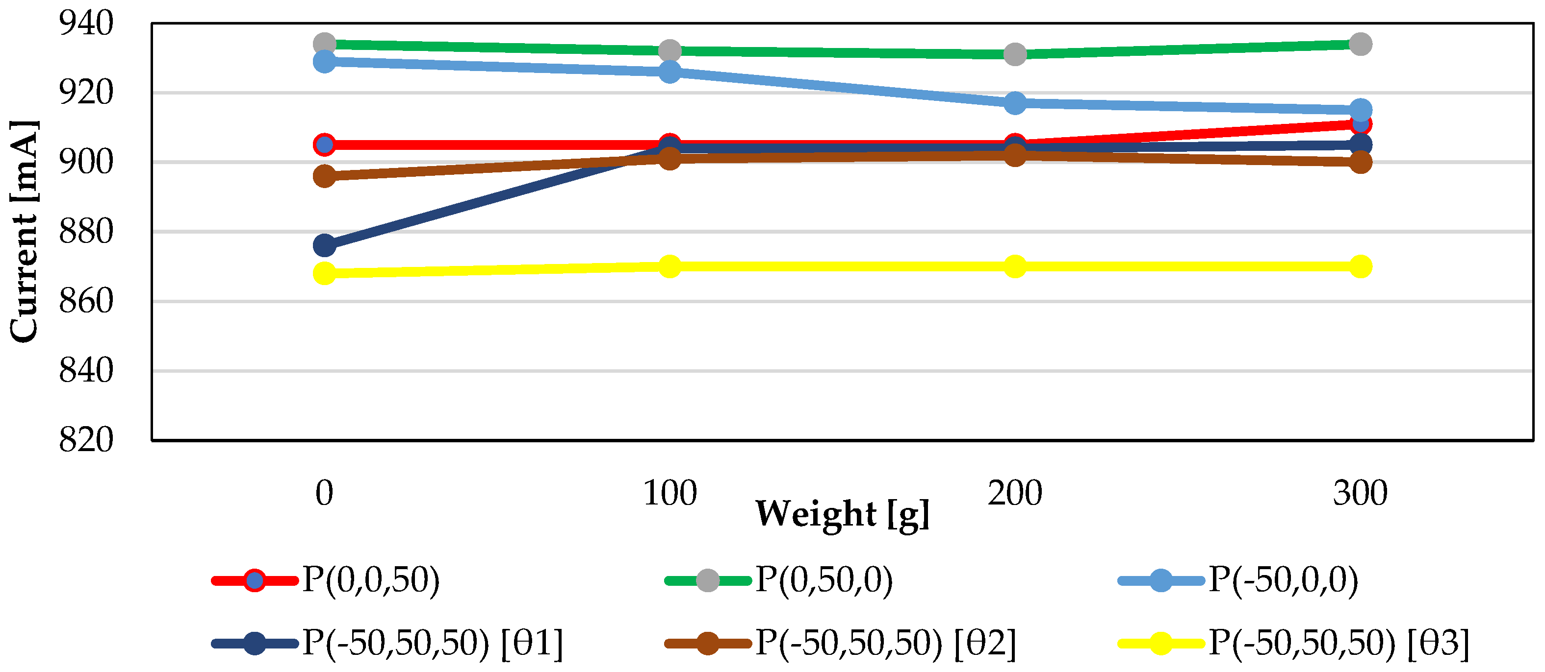
4.4. Test No. 4: Electric Current with Payload Variation

Test no. 4 consisted of verifying the electric current behavior with the load variation (weight) in the effector. Four different positions were selected, and the arm trajectory was always considered starting from the origin position P (0,0,0), being (0,0,0) corresponding to the angle [°] of the three joints. The four positions are: 1—P (−50,0,0), only variation in the axis of joint 1; 2—P (0,50,0), only variation in the axis of joint 2; 3—P (0,0,50), only variation in the axis of joint 3; and 4—P (−50,50,50), variation in the three axes. Figure 17 represents the result of current as a function of weight obtained during test no. 4.

From the analysis shown in Figure 17, it can be concluded that:

-

For a weight less than 100 g, the electric current is low, which means the measured current is influenced by the common mode gain of the amplifier used in the current measurement circuit.

-

It is possible to distinguish the increase in current from the increase in weight (P (0,50,0) and P (0,0,50)), when it is only the movement in only 1 axis of each joint. It was not possible to verify the same for P (−50,0,0), because the current variation was reduced, being influenced by the differential gain.

-

The increase in current with the weight increase during the movement from P (0,0,0) to P (−50,50,50) is not significant because it is a movement in more than one joint; the force exerted depends on the angles of the other joints that are varied. This makes the graph P (0,50,0) different from P (0,50,0) [θ2] and P (0,0,50) different from P (0,0,50) [θ3].

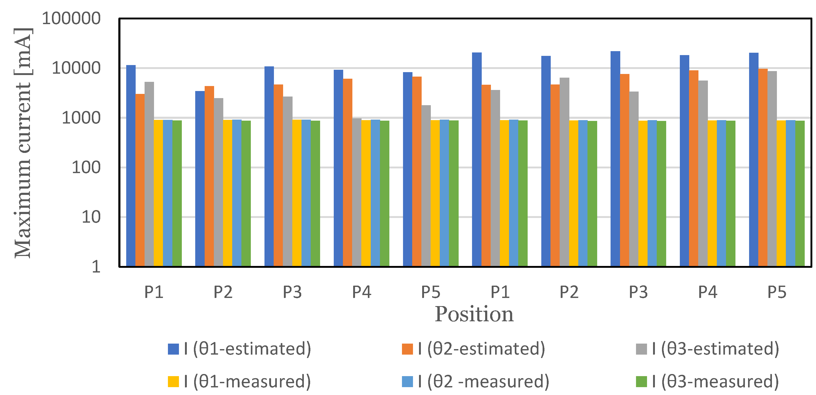
4.5. Test No. 5: Collision Detection

Test no. 5 was the analysis of the technique and method used to detecting collisions. To perform this test, positions were traversed in an automatic mode, in which the trained artificial neural network estimates the maximum current reached in each axis based on the error, the weight attached to the effector and the percentage of execution speed. The network was trained with 290 data obtained with robots in test execution mode. Figure 18 represents the graph with the maximum current estimated by the network and measured during execution.

The first five positions (P1 … P5) during the test were reached with the speed of 20% and a weight of 200 g, and the last five were reached with a speed at 35% and 300 g of weight.

During the test no collision was detected, as expected, but graphically, it is observed that the current estimated by the network increases with increasing weight and speed. In contrast, these values are very high in relation to the current peaks reached during the run, which means the robot cannot detect the collision even if it occurs. The current measured during the test suffered from a little oscillation due to speed and weight, but includes an error associated with the common mode gain of the differential assembly.

Given the unsatisfactory result obtained during the test, and to protect the robotic arm if it collided, the 290 data obtained were used, and the maximum current obtained in each axis was calculated by adding another 2% and defined as the maximum safe current for collision. The maximum safe collision current was set at 946 mA for axis one, 948 mA for axis two and 915 mA for axis three.

5. Conclusions

The development of low-cost collaborative robots was a rather complex project to develop due to the strong practical, control and programming components, and it proved to be a huge challenge to embrace its construction. The project was ambitious due to the amount of work required, since it is a 3D-printed structure based on plastic from the structure and gearbox to the mechanical pinion. During robot development, some constructive problems appeared, such as the issue of having enough space to contain the electronics and ensuring that hidden wiring was not visible.

As for the positioning control, several tests were developed, and great performances of the stepper motor and proposed control method were denoted, presenting a maximum positioning error of 0.035°, when the motor axis locking was ensured by the driver. However, this caused the heating of the motor, which led to the expansion of the pinion that is coupled to the motor shaft, causing mechanical decoupling. When the motion lock is ensured by the torque created by the gearbox (driver disabled), this variation is greater due to the backlash, wear of the girth gear, and the pinion. These variations in both cases tend to increase with the increase in weight attached to the robotic arm.

As for the method and algorithm applied (inverse kinematics), there was always convergence in the solution, which demonstrates the great efficiency of the PSO algorithm; however, this causes errors and a long processing time depending on the predefined parameters.

For most of the current industrial manipulators, repeatability is very high, reaching values below 0.1 mm, while the average precision is around 5 and 15 mm [64]. Table 6 shows that there was a good performance and results in terms of precision, with a maximum error of 0.17 mm in P2. The repeatability error showed acceptable values, with a maximum value in P2 with RP = 0.384 mm.

The method and strategy for collision protection and detection continues to be a challenge in robotics, especially in collaborative robots. The proposed method continues to be a challenge as it requires a lot of test data less associated with error, proposing an optimization of the circuit for electric current measurements.

From the tests that were performed on the three axes of the robotic manipulator, the achievable angles for each axis were: axis 1, −180° to 180°, axis 2, −30° to 210° and axis 3, −160° to 160°. The arm can reach up to 434 mm horizontally and a height of up to 597 mm.

The six-axis, low-cost collaborative robot can be used for educational purposes in different task-specific applications. Several concepts and scientific areas are addressed: the CAD design and 3D printing of the structure, sizing and selection of circuits and/or electronic components, programming, and control. The multidisciplinary approach followed in the development of this cobot allows students from different engineering courses to interact with it and to develop additional features. Moreover, the modular and low-cost technology employed means that students can easily replicate the robot. The technological solution proposed here may be applied in different contexts: education, research, and demonstration. Its main limitations are related to the material used in joint gears that may be easily damaged in collisions. In future research, this model can be used to develop new training curricula, and in that sense, several laboratory training sessions can be developed, from robotics movement fundaments to the inclusion of additional features such as computational vision and artificial intelligence algorithms within practical applications. Thus, the application of technological solutions and scientific and educational approaches used in the development of cobots may foster a wide implementation in Industry 4.0.

Suggestions for Future Work

Due to the scope of this project, some ideas remain unexplored; therefore, some proposals for future work will be listed below. Firstly, some changes in the structure regarding the construction aspect of the arm are suggested to directly contain the electronic components, reinforce the structure to support more weight, increase the power of the motors and resize the gearbox to increase torque. Next, it would be interesting to study the mechanics of the robotic arm in more depth, namely the statics and dynamics. Finally, we programmed and applied other types of movements other than those of the joints, such as linear or circular movements. Additionally, we developed an application for a user interface to enable the movement and control of the robotic arm from mobile devices (tablet, mobile phones, iPad, etc.), or even design and develop a console directly connected to the robotic arm as is the case for marketable robots.

References

1. Haseeb, M.; Hussain, H.I.; Ślusarczyk, B.; Jermsittiparsert, K. Industry 4.0: A Solution towards Technology Challenges of Sustainable Business Performance. Soc. Sci. 2019, 8, 154. [Google Scholar] [CrossRef] [Green Version]
2. Tsaramirsis, G.; Kantaros, A.; Al-Darraji, I.; Piromalis, D.; Apostolopoulos, C.; Pavlopoulou, A.; Alrammal, M.; Ismail, Z.; Buhari, S.M.; Stojmenovic, M.; et al. A Modern Approach towards an Industry 4.0 Model: From Driving Technologies to Management. J. Sensors 2022, 2022, 5023011. [Google Scholar] [CrossRef]
3. IFR. Available online: https://ifr.org/ (accessed on 2 November 2020).
4. Bonilla, S.H.; Silva, H.R.O.; da Silva, M.T.; Gonçalves, R.F.; Sacomano, J.B. Industry 4.0 and Sustainability Implications: A Scenario-Based Analysis of the Impacts and Challenges. Sustainability 2018, 10, 3740. [Google Scholar] [CrossRef] [Green Version]
5. Coşkun, S.; Kayıkcı, Y.; Gençay, E. Adapting Engineering Education to Industry 4.0 Vision. Technologies 2019, 7, 10. [Google Scholar] [CrossRef] [Green Version]
6. Hariharasudan, A.; Kot, S. Review on Digital English and Education 4.0 for Industry 4.0. Soc. Sci. 2018, 7, 227. [Google Scholar] [CrossRef] [Green Version]
7. RIA. Available online: Robotics Online, Robotic Industries Association (accessed on 10 November 2020).
8. ISO/TS 15066:2016(en); Robots and Robotic Devices—Collaborative Robots. International Standards Organization: Geneva, Switzerland, 2016. Available online: https://www.iso.org/obp/ui/#iso:std:iso:ts:15066:ed-1:v1:en (accessed on 12 November 2020).
9. Correia Simões, A.; Lucas Soares, A.; Barros, A.C. Factors Influencing the Intention of Managers to Adopt Collaborative Robots (Cobots) in Manufacturing Organizations. J. Eng. Technol. Manag. 2020, 57, 101574. [Google Scholar] [CrossRef]
10. Zacharaki, A.; Kostavelis, I.; Gasteratos, A.; Dokas, I. Safety Bounds in Human Robot Interaction: A Survey. Saf. Sci. 2020, 127, 104667. [Google Scholar] [CrossRef]
11. Ribeiro, J.P.L.; Gaspar, P.D.; Soares, V.N.G.J.; Caldeira, J.M.L.P. Computational simulation of an agricultural robotic rover for weed control and fallen fruit collection—Algorithms for image detection and recognition and systems control, regulation and command. Electronics 2022, 11, 790. [Google Scholar] [CrossRef]
12. Krimpenis, A.A.; Papapaschos, V.; Bontarenko, E. HydraX, a 3D Printed Robotic Arm for Hybrid Manufacturing. Part I: Custom Design, Manufacturing and Assembly. Procedia Manuf. 2020, 51, 103–108. [Google Scholar] [CrossRef]
13. Stilli, A.; Grattarola, L.; Feldmann, H.; Wurdemann, H.A.; Althoefer, K. Variable Stiffness Link (VSL): Toward Inherently Safe Robotic Manipulators. In Proceedings of the IEEE International Conference on Robotics and Automation (ICRA), Singapore, 29 May–3 June 2017; pp. 4971–4976. [Google Scholar] [CrossRef] [Green Version]
14. Thingiverse WE-R2.4 Six-Axis Robot Arm by LoboCNC. Available online: https://www.thingiverse.com/thing:3327968 (accessed on 23 November 2020).
15. Liu, B.; He, Y.; Kuang, Z. Design and Analysis of Dual-Arm SCARA Robot Based on Stereo Simulation and 3D Modeling. In Proceedings of the 2018 IEEE International Conference on Information and Automation (ICIA), Wuyishan, China, 11–13 August 2018; pp. 1233–1237. [Google Scholar] [CrossRef]
16. Yang, H.; Yan, Y.; Su, S.; Dong, Z.; Ul Hassan, S.H. LWH-Arm: A Prototype of 8-DoF Lightweight Humanoid Robot Arm. In Proceedings of the 2019 3rd IEEE International Conference on Robotics and Automation Sciences (ICRAS), Wuhan, China, 1–3 June 2019; pp. 6–10. [Google Scholar] [CrossRef]
17. Karmoker, S.; Polash, M.M.H.; Hossan, K.M.Z. Design of a Low Cost PC Interface Six DOF Robotic Arm Utilizing Recycled Materials. In Proceedings of the 2014 International Conference on Electrical Engineering and Information & Comunication Technology (ICEEICT), Dhaka, Bangladesh, 10–12 April 2014; pp. 2–6. [Google Scholar] [CrossRef]
18. Sundaram, D.; Sarode, A.; George, K. Vision-Based Trainable Robotic Arm for Individuals with Motor Disability. In Proceedings of the 2019 IEEE 10th Annual Ubiquitous Computing, Electronics and Mobile Communication Conference (UEMCON), New York, NY, USA, 10–12 October 2019; pp. 0312–0315. [Google Scholar] [CrossRef]
19. Liang, X.; Cheong, H.; Sun, Y.; Guo, J.; Chui, C.K.; Yeow, C.H. Design, Characterization, and Implementation of a Two-DOF Fabric-Based Soft Robotic Arm. IEEE Robot. Autom. Lett. 2018, 3, 2702–2709. [Google Scholar] [CrossRef]
20. Dizon, J.R.C.; Espera, A.H.; Chen, Q.; Advincula, R.C. Mechanical Characterization of 3D-Printed Polymers. Addit. Manuf. 2018, 20, 44–67. [Google Scholar] [CrossRef]
21. Stansbury, J.W.; Idacavage, M.J. 3D Printing with Polymers: Challenges among Expanding Options and Opportunities. Dent. Mater. 2016, 32, 54–64. [Google Scholar] [CrossRef] [PubMed]
22. Melchels, F.P.W.; Feijen, J.; Grijpma, D.W. A Review on Stereolithography and Its Applications in Biomedical Engineering. Biomaterials 2010, 31, 6121–6130. [Google Scholar] [CrossRef] [Green Version]
23. Thompson, M.K.; Moroni, G.; Vaneker, T.; Fadel, G.; Campbell, R.I.; Gibson, I.; Bernard, A.; Schulz, J.; Graf, P.; Ahuja, B.; et al. Design for Additive Manufacturing: Trends, Opportunities, Considerations, and Constraints. CIRP Ann. Manuf. Technol. 2016, 65, 737–760. [Google Scholar] [CrossRef] [Green Version]
24. Alfarisi, N.A.S.; Santos, G.N.C.; Norcahyo, R.; Sentanuhady, J.; Azizah, N.; Muflikhun, M.A. Optimization and Performance Evaluation of Hand Cranked Music Box Base Structure Manufactured via 3D Printing. Heliyon 2021, 7, e08432. [Google Scholar] [CrossRef] [PubMed]
25. Kantaros, A.; Piromalis, D. Fabricating Lattice Structures via 3D Printing: The Case of Porous Bio-Engineered Scaffolds. Appl. Mech. 2021, 2, 18. [Google Scholar] [CrossRef]
26. Kantaros, A.; Diegel, O.; Piromalis, D.; Tsaramirsis, G.; Khadidos, A.O.; Khadidos, A.O.; Khan, F.Q.; Jan, S. 3D Printing: Making an Innovative Technology Widely Accessible through Makerspaces and Outsourced Services. Mater. Today Proc. 2021, 49, 2712–2723. [Google Scholar] [CrossRef]
27. All3DP All3DP. Available online: https://all3dp.com/2/pla-vs-abs-filament-3d-printing/ (accessed on 18 July 2021).
28. Hubs. Available online: https://www.hubs.com/knowledge-base/pla-vs-abs-whats-difference/#heat-resistance (accessed on 23 July 2021).
29. Dodziuk, H. Applications of 3D Printing in Healthcare. Kardiochirurg. Torakochirurg. Pol. 2016, 13, 283–293. [Google Scholar] [CrossRef]
30. Nachal, N.; Moses, J.A.; Karthik, P.; Anandharamakrishnan, C. Applications of 3D Printing in Food Processing. Food Eng. Rev. 2019, 11, 123–141. [Google Scholar] [CrossRef]
31. Browne, M.P.; Redondo, E.; Pumera, M. 3D Printing for Electrochemical Energy Applications. Chem. Rev. 2020, 120, 2783–2810. [Google Scholar] [CrossRef]
32. Leitman, S.; Granzow, J. Music Maker: 3d Printing and Acoustics Curriculum. In Proceedings of the 16th International Conference on New Interfaces for Musical Expression (NIME), Brisbane, Australia, 11–15 July 2016; Volume 16, pp. 118–121. [Google Scholar]
33. Telegenov, K.; Tlegenov, Y.; Shintemirov, A. An Underactuated Adaptive 3D Printed Robotic Gripper. In Proceedings of the 10th France-Japan/8th Europe-Asia Congress on Mecatronics, Tokyo, Japan, 27–29 November 2014; pp. 110–115. [Google Scholar] [CrossRef]
34. Chinthavali, M. 3D Printing Technology for Automotive Applications; Oak Ridge National Laboratory: Oak Ridge, TN, USA, 2016. [Google Scholar]
35. Zhang, S.; Vardaxoglou, Y.; Whittow, W.; Mittra, R. 3D-Printed Flat Lens for Microwave Applications. In Proceedings of the 2015 Loughborough Antennas and Propagation Conference (LAPC), Loughborough, UK, 2–3 November 2015; pp. 31–33. [Google Scholar] [CrossRef] [Green Version]
36. Chen, G.; Xu, Y.; Kwok, P.C.L.; Kang, L. Pharmaceutical Applications of 3D Printing. Addit. Manuf. 2020, 34, 101209. [Google Scholar] [CrossRef]
37. Nadagouda, M.N.; Ginn, M.; Rastogi, V. A Review of 3D Printing Techniques for Environmental Applications. Curr. Opin. Chem. Eng. 2020, 28, 173–178. [Google Scholar] [CrossRef] [PubMed]
38. Blachowicz, T.; Pająk, K.; Recha, P.; Ehrmann, A. 3D Printing for Microsatellites-Material Requirements and Recent Developments. AIMS Mater. Sci. 2020, 7, 926–938. [Google Scholar] [CrossRef]
39. Babiuch, M.; Foltynek, P.; Smutny, P. Using the ESP32 Microcontroller for Data Processing. In Proceedings of the 2019 20th International Carpathian Control Conference (ICCC), Krakow/Wieliczka, Poland, 26–29 May 2019. [Google Scholar] [CrossRef]
40. Bipasha Biswas, S.; Tariq Iqbal, M. Solar Water Pumping System Control Using a Low Cost ESP32 Microcontroller. In Proceedings of the 2018 IEEE Canadian Conference on Electrical and Computer Engineering, Quebec, QC, Canada, 13–16 May 2018; pp. 7–11. [Google Scholar] [CrossRef]
41. Bunkum, M.; Vachirasakulchai, P.; Nampeng, J.; Tommajaree, R.; Visitsattapongse, S. Tele-Operation of Robotic Arm. In Proceedings of the 2019 12th Biomedical Engineering International Conference (BMEiCON), Ubon Ratchathani, Thailand, 19–22 November 2019. [Google Scholar] [CrossRef]
42. Bolla, D.R.; Jijesh, J.J.; Palle, S.S.; Penna, M.; Keshavamurthy, S. An IoT Based Smart E-Fuel Stations Using ESP-32. In Proceedings of the 5th IEEE International Conference on Recent Trends on Electronics, Information and Communication Technology (RTEICT), Bangalore, India, 12–13 November 2020; pp. 333–336. [Google Scholar] [CrossRef]
43. Rai, P.; Rehman, M. ESP32 Based Smart Surveillance System. In Proceedings of the 2019 2nd International Conference on Computing, Mathematics and Engineering Technologies (iCoMET), Sukkur, Pakistan, 30–31 January 2019; pp. 8–10. [Google Scholar] [CrossRef]
44. Contardi, U.A.; Morikawa, M.; Brunelli, B.; Thomaz, D.V. MAX30102 Photometric Biosensor Coupled to ESP32-Webserver Capabilities for Continuous Point of Care Oxygen Saturation and Heartrate Monitoring. Eng. Proc. 2022, 16, 1114. [Google Scholar] [CrossRef]
45. Espressif. Available online: https://www.espressif.com/en/products/socs/esp32 (accessed on 1 August 2021).
46. 3D Lab 3D Lab. Available online: https://3dlab.com.br/10-softwares-de-modelagem-3d/ (accessed on 19 October 2021).
47. Arduino. Available online: https://www.arduino.cc/en/Guide/Environment (accessed on 18 October 2021).
48. MATLAB. Available online: https://www.mathworks.com/products/matlab.html (accessed on 19 October 2021).
49. Spatial Transformation Matrices Spatial Transformation Matrices. Available online: https://www.brainvoyager.com/bv/doc/UsersGuide/CoordsAndTransforms/SpatialTransformationMatrices.html (accessed on 19 October 2021).
50. Dasari, A.; Reddy, N.S. Forward and Inverse Kinematics of a Robotic Frog. In Proceedings of the 4th International Conference on Intelligent Human Computer Interaction (IHCI), Kharagpur, India, 27–29 December 2012. [Google Scholar] [CrossRef]
51. Spong, M.W.; Hutchinson, S.; Vidyasagar, M. Robot Modeling and Control, 2nd ed.; John Wiley & Sons: New York, NY, USA, 2020; ISBN 978-1-119-52404-5. [Google Scholar]
52. Fernández, E.F.; Almonacid, F.; Sarmah, N.; Rodrigo, P.; Mallick, T.K.; Pérez-Higueras, P. A Model Based on Artificial Neuronal Network for the Prediction of the Maximum Power of a Low Concentration Photovoltaic Module for Building Integration. Sol. Energy 2014, 100, 148–158. [Google Scholar] [CrossRef]
53. Talari, S.; Shafie-khah, M.; Chen, Y.; Wei, W.; Gaspar, P.D.; Catalão, J.P.S. Real-Time Scheduling of Demand Response Options Considering the Volatility of Wind Power Generation. IEEE Trans. Sustain. Energy 2019, 10, 1633–1643. [Google Scholar] [CrossRef]
54. Gomes, D.E.; Iglésias, M.I.D.; Proença, A.P.; Lima, T.M.; Gaspar, P.D. Applying a Genetic Algorithm to an m-TSP: Case Study of a Decision Support System for Optimizing a Beverage Logistics Vehicles Routing Problem. Electronics 2021, 10, 2298. [Google Scholar] [CrossRef]
55. Freitas, A.A.; Lima, T.M.; Gaspar, P.D. Meta-Heuristic Model for Optimization of Production Layouts Based on Occupational Risk Assessment: Application to the Portuguese Wine Sector. Appl. Syst. Innov. 2022, 5, 40. [Google Scholar] [CrossRef]
56. Freitas, A.A.; Lima, T.M.; Gaspar, P.D. Ergonomic Risk Minimization in the Portuguese Wine Industry: A Task Scheduling Optimization Method Based on the Ant Colony Optimization Algorithm. Processes 2022, 10, 1364. [Google Scholar] [CrossRef]
57. Mesquita, R.; Gaspar, P.D. A Novel Path Planning Optimization Algorithm Based on Particle Swarm Optimization for UAVs for Bird Monitoring and Repelling. Processes 2021, 10, 62. [Google Scholar] [CrossRef]
58. Magalhães, B.; Gaspar, P.D.; Corceiro, A.; João, L.; Bumba, C. Fuzzy Logic Decision Support System to predict Peaches Marketable Period at Highest Quality. Climate 2022, 10, 29. [Google Scholar] [CrossRef]
59. Ananias, E.; Gaspar, P.D.; Soares, V.N.G.J.; Caldeira, J.M.L.P. Artificial Intelligence Decision Support System Based on Artificial Neural Networks to Predict the Commercialization Time by the Evolution of Peach Quality. Electronics 2021, 10, 2394. [Google Scholar] [CrossRef]
60. Alibabaee, K.; Gaspar, P.D.; Lima, T. Crop Yield Estimation using Deep Learning Based on Climate Big Data. Energies 2021, 14, 3004. [Google Scholar] [CrossRef]
61. Alibabaei, K.; Gaspar, P.D.; Lima, T.; Campos, R.M.; Girão, I.; Monteiro, J.; Lopes, C.M. A Review of the Challenges of using Deep Learning Algorithms to Support Decision-Making in Agricultural Activities. Remote Sens. 2022, 14, 638. [Google Scholar] [CrossRef]
62. Alkayyali, M.; Tutunji, T.A. PSO-Based Algorithm for Inverse Kinematics Solution of Robotic Arm Manipulators. In Proceedings of the 2019 20th International Conference on Research and Education in Mechatronics (REM), Wels, Austria, 23–24 May 2019; Volume 5, pp. 8–13. [Google Scholar] [CrossRef]
63. ISO 9283:1998(en); Manipulating Industrial Robots—Performance Criteria and Related Test Methods. 2nd ed. International Standards Organization: Geneva, Switzerland, 1998.
64. Abderrahim, M.; Khamis, A.; Garrido, S.; Moreno, L. Accuracy and Calibration Issues of Industrial Manipulators. In Industrial Robotics: Programming, Simulation and Application; pIV pro literature Verlag: Mammendorf, Germany, 2006. [Google Scholar] [CrossRef] [Green Version]
Figure 1. Numbers (×1000) of industrial robots installed per year [3].
Asi 05 00072 g001
Figure 2. Annual evolution of the acquisition (×1000) of collaborative robots versus traditional robots [3].
Asi 05 00072 g002
Figure 3. Representation of the homogeneous matrix.
Asi 05 00072 g003
Figure 4. Artificial neural network typical architecture.
Asi 05 00072 g004
Figure 5. (a) Conical base of the manipulator; (b) toothed ring; (c) shoulder; (d) extension arm; (e) toothed ring with motor mount; (f) secondary double pinion; (g) shoulder pad; (h) main single pinion; (i) toothed wheel; (j) robotic arm.
Asi 05 00072 g005
Figure 6. Kinematics of the robotic manipulator.
Asi 05 00072 g006
Figure 7. This pseudo code for PSO meta heuristics.
Asi 05 00072 g007
Figure 8. Diagram and typology of communication between ESP32 and PC.
Asi 05 00072 g008
Figure 9. Connection diagram between devices of each axis.
Asi 05 00072 g009
Figure 10. (a) PCB developed and printed: top view; (b) PCB designed and printed: bottom view; (c) PCB designed with soldered components: top view; (d) PCB designed with soldered components: bottom view.
Asi 05 00072 g010
Figure 11. Ramp of number of pulses applied to the motor as a function of error.
Asi 05 00072 g011
Figure 12. User interface; connect menu.
Asi 05 00072 g012
Figure 13. User interface; move menu.
Asi 05 00072 g013
Figure 14. User interface; control menu.
Asi 05 00072 g014
Figure 15. Final assembled robotic arm.
Asi 05 00072 g015
Figure 16. (a) Position plan for test no. 3; (b) Sequence of movement.
Asi 05 00072 g016
Figure 17. Current result as a function of weight obtained during test no. 4.
Asi 05 00072 g017
Figure 18. The result of the maximum current estimated and measured during test no. 5.
Asi 05 00072 g018