1. Introduction
Electronic devices and services such as mobile phones, hearing aids, headphones, and teleconference systems play a significant role in our lives. In particular, voice-based functions and applications (voice interaction, voice communication, and speech recognition) are essential in these devices and services. However, various sources of interference exist that deteriorate speech signals during transmission, and thus they undermine the capability of the functions mentioned above and applications. These interference sources include additive noise, channel distortion, and reverberation. In order to alleviate the influence of interference, various methods have been presented in recent decades from different perspectives of speech processing systems, such as front-end signal processing, acoustic feature design, and back-end acoustic modeling. Roughly speaking, the methods regarding the front-end acoustic signal-domain processing belong to speech enhancement (SE). In contrast, the techniques for the acoustic features and models are related to robust speech recognition.
According to [
1], speech enhancement (SE) algorithms can be divided into four categories: spectral-subtractive [
1,
2,
3], statistical modeling [
1,
4,
5,
6,
7], sub-space based [
1,
8,
9], and masking-based [
10,
11,
12]. In particular, due to the successful development of deep neural network (DNN) techniques in the recent decade, the modeling of speech enhancement algorithms and the respective procedures (such as noise estimation and sub-space basis extraction) are significantly upgraded to achieve even better performance. For example, a DNN can be used to learn the statistical relationship between noisy utterances and clean counterparts through a massive amount of noisy–clean utterance pairs in a prepared training set. In particular, since speech enhancement aims to transform noisy speech back to clean speech, which is a standard regression problem in machine/deep learning, the mean squared error (MSE) loss function is often used in the SE-wise DNN.
However, when it comes to the performance evaluation of a speech enhancement algorithm, some objective metrics, such as the perceptual evaluation of speech quality (PESQ) [
13] and short-time objective intelligibility (STOI) [
14], are often used. These metrics are not necessarily related to the mean squared distance between the enhanced and original clean speech. Therefore, in some recently developed deep-learning-based SE algorithms [
15,
16], PESQ and STOI are employed directly to be the objective functions for the training of DNN models.
PESQ is a standard objective metric to measure speech quality, recommended by ITU-T. It is developed to predict the mean opinion scores (MOS) in subjective listening tests, and according to [
17], PESQ shows a high correlation
with MOS. PESQ is widely used to evaluate speech separation and enhancement algorithms. It mainly quantizes speech quality by computing the disturbance between the clean and separated/enhanced speech using cognitive modeling. PESQ ranges within [−0.5, 4.5], with high values indicating better quality [
13,
18].
Here, we provide a little more discussion about the issue that using mean squared error (MSE) as the loss function in most deep-learning-based SE algorithms [
10,
19,
20,
21] does not necessarily give rise to higher PESQ/STOI scores in the processed utterances. According to [
18,
21], two fundamental assumptions of the MSE loss in these SE methods somewhat contradict human auditory perception, which are as follows:
Every estimated element is equally important [18]: The MSE loss function treats each single data point equally. Regardless of the locations of the processed data, the same difference between the elements of each processed output and the desired output corresponds to the equal MSE loss value. The underlying reason is that the MSE loss is derived from each sample point of the utterance separately and independently instead of the whole utterance trajectory. However, we evaluate the quality and intelligibility of an utterance in a different manner. For example, the speech-dominant portion is treated more crucially than the silence portion in the STOI metric.
In contrast, the PESQ metric pays more attention to isolated samples because they are more involved with speech quality. In addition, when considered in the frequency domain, the MSE loss is usually defined at the linear frequency scale. At the same time, the speech quality/intelligibility metrics are measured at human auditory frequency scales (such as the mel scale and Bark scale). To sum up, minimizing the MSE loss is not necessary to optimize the PESQ or STOI scores for noisy utterances.
The optimal solution is determined by the whole utterance set [21]: To extend the idea of the previous point, using the MSE as the objective loss function tends to consider the portions in utterances with different characteristics in an averaged manner, which might alleviate the distinct and discriminative components that highlight the speech. For example, an ordinary utterance set possesses low- and high-pitch utterances. Minimizing the MSE at these utterances indiscriminately very likely causes these utterances to have median pitches, which is not our goal at all.
Inspired by the observations mentioned above and some other literature [
15,
18,
22], in this study, we propose a novel deep-learning-based noise-robust speech feature extraction algorithm with an MSE-irrelevant loss function. The used loss function is directly associated with the performance of a speech recognition system in noisy environments. Briefly speaking, a deep neural network is trained to perform the speech feature mapping that maximizes the posterior state probability associated with the back-end acoustic models in the speech recognition system. The resulting new speech feature representation is expected to outperform the original feature in recognition accuracy and possess noise robustness.
It is noteworthy that many research efforts have employed deep neural networks to engage in an ASR system to improve its noise robustness. For example, an end-to-end (E2E) ASR framework with a single DNN directly maps an acoustic feature sequence to a word sequence [
23,
24,
25]. This E2E DNN is learned to optimize criteria directly associated with the ASR performance, such as the word error rate (WER). Such an E2E model can behave better and be more compact than the conventional hybrid ASR model, consisting mainly of acoustic models, a lexicon, and language models. The authors in [
26] claim that the improvements in speech quality metrics such as PESQ by speech enhancement techniques do not translate into better ASR performance. They propose a joint optimization of mask-estimating network-based speech enhancement and acoustic modeling to reduce the WER. In addition, a deep learning scheme for
a priori SNR estimation, termed Deep Xi, is presented in [
27,
28] to facilitate the conventional minimum-mean-squared-error (MMSE)-based SE methods for a robust ASR. Compared with these complicated and fine-grained techniques, our newly presented method is a relatively lightweight network that is much easier to be learned, while it is likely less effective. However, our method is a DNN-wise transformation in the same feature domain and thus can be easily integrated with these advanced methods to boost the ASR performance.
In the following sections, we first introduce the original acoustic features and the associated acoustic models in a pre-processing stage and then present the novel feature extraction algorithm. Next, we compare our method with various speech features created by the utterances enhanced by some state-of-the-art enhancement methods. Finally, we give a concluding remark.
4. The Evaluation Results and Discussions
This section provides a series of experiments to evaluate the presented new noise-robust speech feature extraction method. The experimental setup is given in
Section 4.1, and the recognition results achieved by some well-known speech enhancement methods are given and discussed in
Section 4.2. Finally,
Section 4.3 and
Section 4.4 present and analyze the presented method’s results as well as several comparative algorithms.
4.1. The Experimental Setup
In the following, we describe the used data corpus, the ASR system preparation, and the arrangement of the DNN for our presented method.
4.1.1. Data Corpus
We used the well-known TIMIT corpus [
37] to experiment. TIMIT contains phonemically and lexically transcribed speech utterances from American English speakers of different genders and dialects. These utterances correspond to the broadband recordings of 630 speakers of eight major dialects of American English, each speaker reading ten phonetically rich sentences. Each utterance is a 16-bit, 16 kHz sampling rate waveform file accompanied by time-aligned orthographic, phonetic, and word transcriptions. The utterances in TIMIT were used as the training and test sets in our evaluation experiments. As for the multi-condition training set, 1000 utterances were randomly selected and corrupted with any of three noise types (babble, car, and street) at five
signal-to-noise ratio (SNR) levels (−5 dB, 0 dB, 5 dB, 10 dB, and 15 dB). For the test set, 400 utterances different from the training set were selected and corrupted with any of three noise types (white, engine, and jackhammer) at six SNR levels (−6 dB, −3 dB, 0 dB, 3 dB, 6 dB, and 12 dB). In the experiments, we tested the utterances with respect to each noise type and each SNR level to see the detailed effects of the evaluated methods.
4.1.2. The ASR System Preparation
The speech features in the training set were used to learn context-dependent (CD) tri-phones as acoustic models, which were arranged to be two different structures, i.e., GMM-HMM and DNN-HMM, respectively. Stating in more detail, GMM-HMM and DNN-HMM used GMM and DNN, respectively, to represent each state of the HMM. As for GMM-HMM, each mono-phone of speech signals and the silence were respectively characterized by an HMM with three states, having 1000 Gaussians in total, and each tri-phone was characterized by an HMM with three states, having 2500 leaves and 1500 Gaussians in total. Furthermore, LDA, MLLT, SAT were applied to the speech features during the tri-phone model training. On the other hand, for the DNN structure, five hidden layers, each containing 1024 nodes with a dropout rate
, were connected to two independent output layers for tri-phones and mono-phones, respectively, in the DNN-HMM. The training process of this DNN underwent 24 epochs with an SGD optimizer and used the log-likelihood loss function for tri-phones and mono-phones. The losses of tri-phones and mono-phones were added up for minimization in the model training. The Kaldi toolkit [
32] was used to create the GMM-HMM and the Pytorch-Kaldi [
38] toolkit was used to create the DNN-HMM.
In addition, a set of tri-gram language models for training utterances was created via following the standard recipes of Kaldi.
4.1.3. The DNN Structure for Denoising Feature Extraction
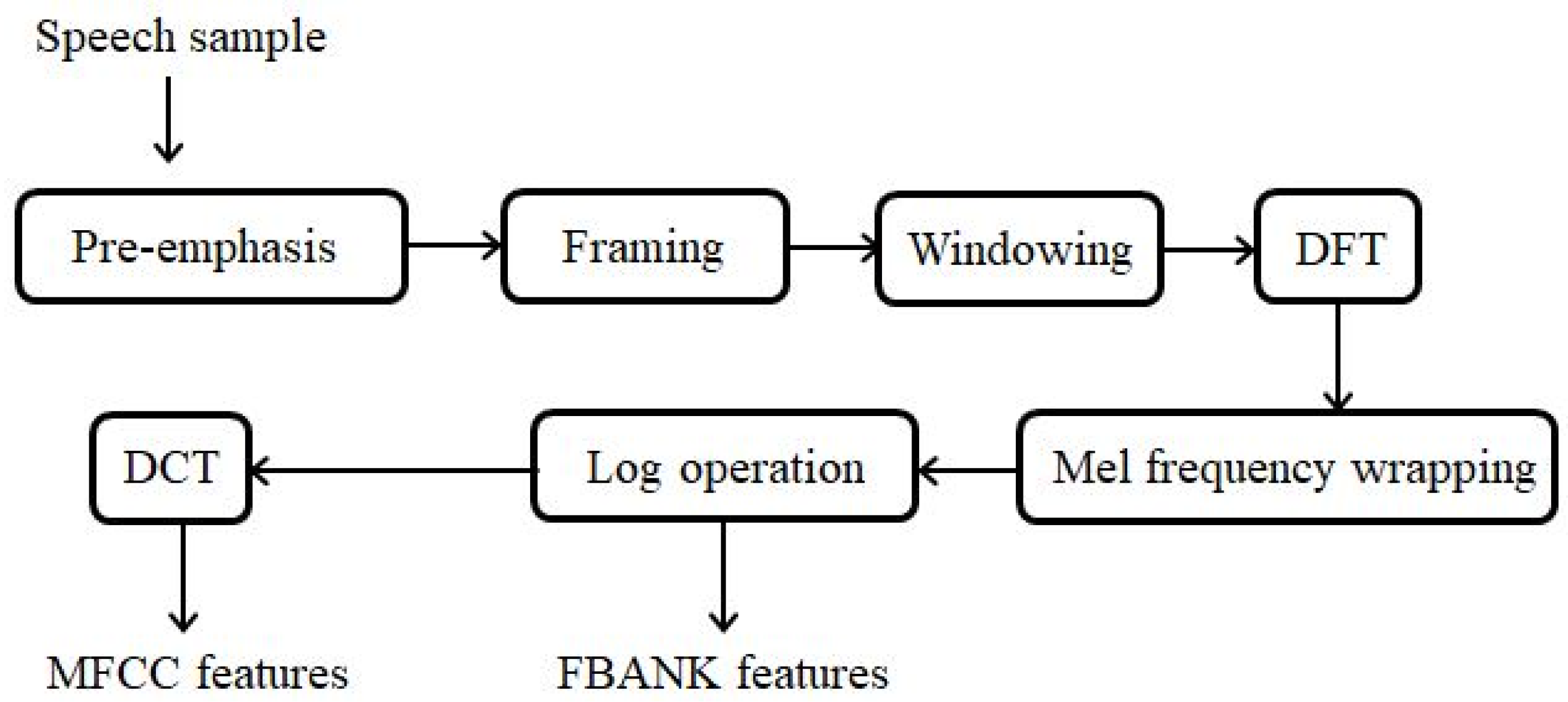
For each of the utterances in the training and test set, the 69-dimensional FBANK feature stream (23 static FBANKs together with their delta and delta-delta for each frame, with a 20 ms frame duration and a 10 ms frame shift) was created as the baseline feature representation. The presented denoising DNN framework took the FBANK as input to produce the updated feature following the procedures in
Section 3.1 for the subsequent recognition. The denoising DNN model was a convolutional neural network (CNN) with four same-size one-dimensional convolutional layers, each following a configuration setting (30, 5, 2), where the setting representation was “(number of kernel, kernel size, number of padding)”. In addition, these four convolutional layers were followed by the two same fully connected layers with 759 nodes. The activation function for each layer output was the rectified linear unit (ReLU). The training process of this denoising framework underwent 30 epochs with the Adam optimizer and used the log-likelihood loss function.
4.2. The Effect of SE Methods in Speech Recognition for Noisy Speech
In this subsection, we would like to investigate whether the signals pre-enhanced by speech enhancement (SE) methods can result in speech features that bring about improved recognition accuracies relative to the baseline. We selected two SE methods: MMSE [
39] (an unsupervised approach) and ideal ratio mask (IRM) [
10] (a supervised approach) and conducted the evaluation experiments with a multi-condition mode in two different arrangements:
- (1)
The SE process was conducted on the utterances in both the training and test sets.
- (2)
The SE process was only conducted on the utterances in the test set, while the training set remained unchanged.
Table 1,
Table 2 and
Table 3 list the word error rates (WER in %) for the above two arrangements with respect to the test utterances of three noise types (white, engine, and jackhammer). In these tables, MMSE (TR, TS) and IRM (TR, TS) refer to the first arrangement, in which both the training and test sets were enhanced by MMSE/IRM, while MMSE (TS) and IRM (TS) refer to the second arrangement, in which MMSE/IRM enhanced only the test set. Furthermore, to see if the two SE methods can improve the quality and intelligibility of the test utterances as they promise, we also list the PESQ and STOI scores in these tables. From the results shown in these three tables, we have the following observations:
Both MMSE and IRM improve the PESQ scores, while MMSE behaves better than IRM in most cases. For example, MMSE obtains 1.647 and 1.967 in PESQ at the 12 dB SNR case of
Table 1 and
Table 2, while the corresponding values achieved by IRM are 1.275 and 1.493. This is possibly due to the mismatch between the training and test sets for IRM. However, neither MMSE nor IRM can bring a significant STOI upturn for almost all noise scenarios. In addition, IRM results in less STOI degradation than MMSE.
Comparing the two first arrangements (“TR, TS” and “TS”) as for MMSE and IRM, we find that conducting the SE methods on both the training and test sets shows inferior recognition performance (higher WERs) than conducting them only on the test set. Furthermore, the first arrangement “TR, TS” even causes worse results than the baseline. For example, the methods “MMSE (TR, TS)” and “MMSE (TS)” obtain
and
WERs at the 3 dB SNR case of
Table 1, which are worse than the baseline
. The underlying explanation is that MMSE and IRM, when conducted on the training set, result in an over-smooth trajectory for speech utterances in the time or spectral domains and therefore reduce the diversity and discriminant capability of the various phone realizations in the training set.
As for the second arrangement (i.e., MMSE and IRM conducted only on the test set), IRM appears to bring moderately lower WERs for the two noise types “white” and “engine” (shown in the lower part of
Table 1 and
Table 2), while it is not quite helpful for the “jackhammer” case (shown in the lower part of
Table 3). Comparatively, MMSE worsens the recognition accuracy for all three noise situations.
Based on the above observations, we may conclude with the following points:
The two metrics, PESQ and WER, seem to have little correlation since the method MMSE, which causes better PESQ scores, results in higher WERs (except for some low SNR cases). That is, improving the speech quality does not necessarily reduce its recognition accuracy. Relative to PESQ, the STOI index has more to do with the recognition accuracy in more noisy situations. This can be observed in that the method IRM can improve STOI and recognition accuracy simultaneously for “white” and “engine” noises, even though the improvement is somewhat marginal. In addition, the increase in STOI does not necessarily reduce WER, while the reduction in WER always comes with the increase in STOI.
The two SE methods used here do not show obvious benefits of speech recognition in noisy situations. In our opinion, directly compensating speech features used for a noisy recognition system is probably more helpful in reducing WERs than enhancing speech signals by SE methods.
Table 1.
The various evaluation results of MMSE, IRM, and the baseline for the test set in noise environment “white”. The results worse than the baseline are marked with a superscript “*”. In particular, we also give the same marking for the results worse than the baseline in the other tables.
Table 1.
The various evaluation results of MMSE, IRM, and the baseline for the test set in noise environment “white”. The results worse than the baseline are marked with a superscript “*”. In particular, we also give the same marking for the results worse than the baseline in the other tables.
| | | Signal-To-Noise Ratio (SNR) |
|---|
| | | −6 dB | −3 dB | 0 dB | 3 dB | 6 dB | 12 dB |
| | baseline | 1.031 | 1.036 | 1.044 | 1.062 | 1.096 | 1.271 |
| PESQ | MMSE | 1.040 | 1.054 | 1.080 | 1.130 | 1.237 | 1.647 |
| | IRM | 1.032 | 1.036 | 1.044 | 1.063 | 1.098 | 1.275 |
| | baseline | 0.577 | 0.648 | 0.722 | 0.790 | 0.850 | 0.935 |
| STOI | MMSE | 0.584 | 0.643 * | 0.697 * | 0.734 * | 0.766 * | 0.840 * |
| | IRM | 0.578 | 0.649 | 0.723 | 0.792 | 0.852 | 0.937 |
| | baseline | 66.1 | 62.1 | 57.0 | 49.8 | 44.8 | 34.4 |
| | MMSE (TR, TS) | 70.0 * | 66.7 * | 61.9 * | 56.5 * | 50.5 * | 40.5 * |
| WER (%) | IRM (TR, TS) | 67.3 * | 63.1 * | 58.3 * | 52.5 * | 47.3 * | 37.5 * |
| | MMSE (TS) | 70.3 * | 66.8 * | 60.4 * | 55.0 * | 49.7 * | 40.1 * |
| | IRM (TS) | 65.8 | 61.9 | 56.5 | 50.4 | 44.4 | 34.3 |
Table 2.
The various evaluation results of MMSE, IRM, and the baseline for the test set in noise environment “engine”.
Table 2.
The various evaluation results of MMSE, IRM, and the baseline for the test set in noise environment “engine”.
| | | Signal-To-Noise Ratio (SNR) |
|---|
| | | −6 dB | −3 dB | 0 dB | 3 dB | 6 dB | 12 dB |
| | baseline | 1.051 | 1.064 | 1.087 | 1.128 | 1.195 | 1.482 |
| PESQ | MMSE | 1.103 | 1.103 | 1.198 | 1.350 | 1.520 | 1.967 |
| | IRM | 1.051 | 1.064 | 1.087 | 1.128 | 1.195 | 1.493 |
| | baseline | 0.506 | 0.575 | 0.651 | 0.726 | 0.796 | 0.899 |
| STOI | MMSE | 0.515 | 0.579 | 0.638 * | 0.692 * | 0.743 * | 0.850 * |
| | IRM | 0.506 | 0.575 | 0.652 | 0.726 | 0.796 | 0.901 |
| | baseline | 65.3 | 61.7 | 55.1 | 48.2 | 41.5 | 31.1 |
| | MMSE (TR,TS) | 68.2 * | 63.8 * | 57.8 * | 51.4 * | 44.3 * | 32.6 * |
| WER (%) | IRM (TR,TS) | 67.5 * | 64.7 * | 59.0 * | 52.9 * | 46.0 * | 35.3 * |
| | MMSE (TS) | 68.3 * | 63.6 * | 57.3 * | 51.4 * | 44.9 * | 34.2 * |
| | IRM (TS) | 65.9 * | 61.4 | 54.8 | 48.2 | 41.2 | 31.1 |
Table 3.
The various evaluation results of MMSE, IRM, and the baseline for the test set in noise environment “jackhammer”.
Table 3.
The various evaluation results of MMSE, IRM, and the baseline for the test set in noise environment “jackhammer”.
| | | Signal-To-Noise Ratio (SNR) |
|---|
| | | −6 dB | −3 dB | 0 dB | 3 dB | 6 dB | 12 dB |
| | baseline | 1.682 | 1.946 | 2.242 | 2.566 | 2.919 | 3.533 |
| PESQ | MMSE | 2.087 | 2.413 | 2.739 | 3.059 | 3.323 | 3.812 |
| | IRM | 1.773 | 2.044 | 2.350 | 2.680 | 3.024 | 3.624 |
| | baseline | 0.924 | 0.950 | 0.968 | 0.981 | 0.989 | 0.997 |
| STOI | MMSE | 0.917 * | 0.944 * | 0.962 * | 0.976 * | 0.983 * | 0.991 * |
| | IRM | 0.932 | 0.955 | 0.970 | 0.982 | 0.990 | 0.997 |
| | baseline | 31.4 | 27.8 | 25.9 | 23.8 | 23.0 | 21.9 |
| | MMSE (TR,TS) | 32.3 * | 28.7 * | 26.4 * | 24.5 * | 23.9 * | 22.5 * |
| WER (%) | IRM (TR,TS) | 33.6 * | 30.4 * | 27.4 * | 25.2 * | 24.1 * | 22.9 * |
| | MMSE (TS) | 32.9 * | 29.0 * | 27.2 * | 25.2 * | 24.4 * | 23.2 * |
| | IRM (TS) | 32.4 * | 29.8 * | 26.6 * | 25.2 * | 23.8 * | 22.8 * |
4.3. Experimental Results and Discussions for the Proposed Method
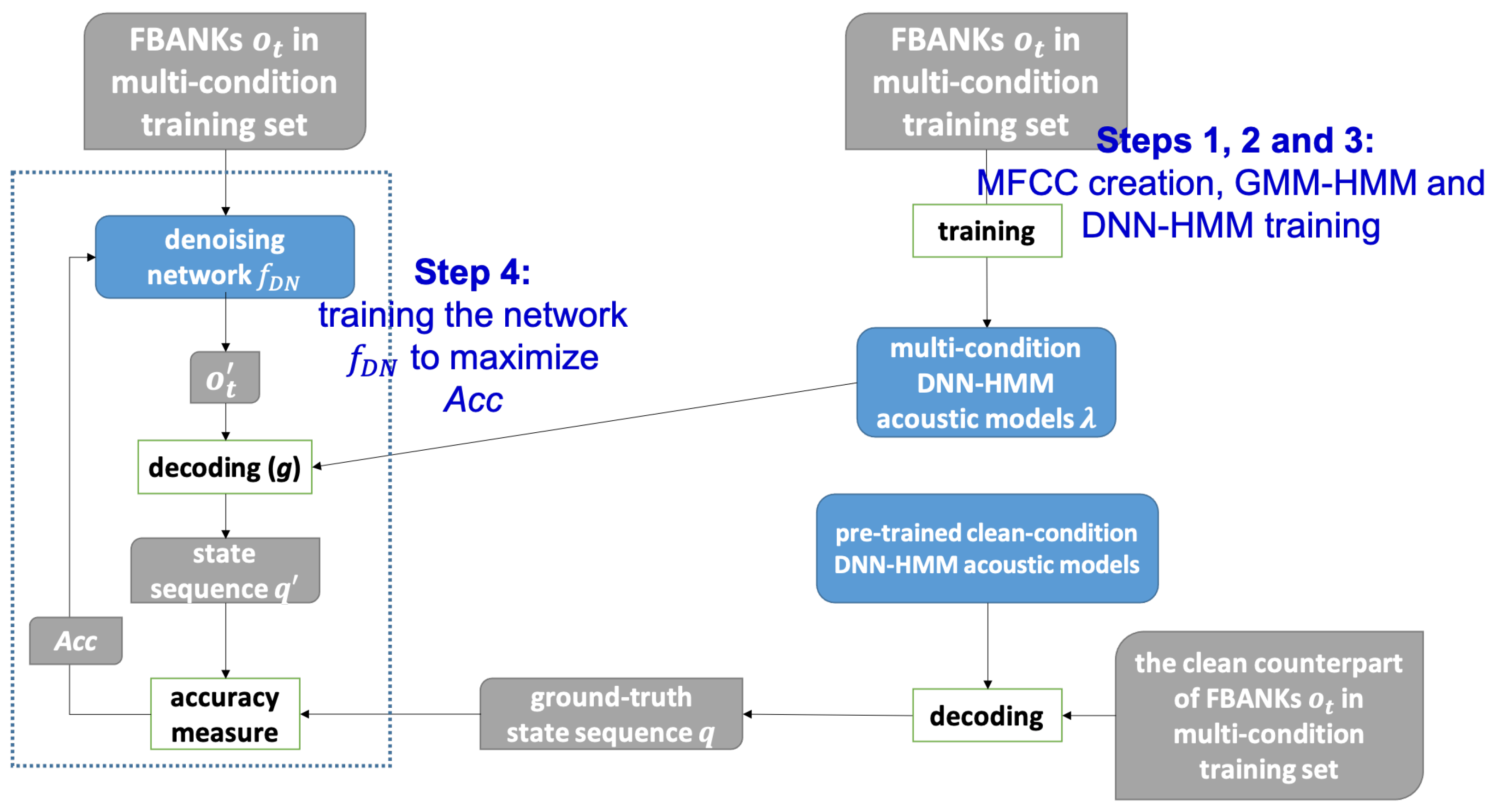
In this subsection, we provide the experimental results of our presented method and some discussions. For ease of discussion, the presented method is termed “maximum state posterior probability” with the abbreviation “MSPP”. The experimental results for the multi-condition test utterances are further split into two parts: multi-condition training mode and clean-condition training mode. Note that the denoising framework in our method is with the help of the multi-condition training set, but we would like to see if the resulting enhanced speech features can behave well in both modes.
Furthermore, we employ a comparative method for evaluation which primarily uses a deep neural network (DNN) to update the input FBANK features. This DNN is learned by directly minimizing the mean squared error (MSE) between the noisy and clean FBANK feature pairs in the multi-condition training set. This comparative method is termed feature-based MSE and abbreviated by “FMSE” in the following discussions.
Before going into the experimental results, it is worth noting again that we used the original plain FBANK in the training set to prepare the acoustic models for both multi-condition and clean-condition training modes. Therefore, the various speech enhancement/robust feature extraction methods were just conducted on the test sets.
4.3.1. Multi-Condition Training Mode
Table 4,
Table 5 and
Table 6 list the WER (%) for our method, MSPP, and FMSE, together with the two SE methods (MMSE and IRM) in the preceding sub-section
using the acoustic models learned from the multi-condition training set. The used acoustic models are common to the four comparative methods. Since the presented MSPP is directly related to state posteriors in the acoustic models, here we also list the state error rates with the various methods for the test utterances. From these three tables, we have the following observations:
On average,
Table 6 shows that the WERs achieved by various methods in the jackhammer noise environment are significantly lower than those in the white and engine noise environments as in
Table 4 and
Table 5, indicating that jackhammer noise brings less distortion to speech signals compared with the white and engine noises. However, we find that all of the used methods here fail to outperform the baseline results for the jackhammer noise case, indicating that the speech enhancement/noise-robust feature methods might introduce further observable distortion to less contaminated utterances.
As for the white and engine noise situations as in
Table 4 and
Table 5, the newly proposed MSPP can achieve lower WERs in most SNR cases and outperform the other methods in comparison, which clearly validates the main thought of MSPP that increasing the state posteriors helps to improve the noise robustness and promote recognition accuracy. For example, observing the the lower part of
Table 4 and
Table 5, MSPP achieves
and
WER at 0 dB SNR for white and engine noise cases, better than the baseline results
and
. In particular, the denoising framework in the presented MSPP is created upon the noisy dataset in which noise types are neither white nor engine. Thus, MSPP is shown to have a generalization capability to conquer unseen noise.
When observing the state error rates achieved by the various methods as shown in the upper parts of
Table 4,
Table 5 and
Table 6, we do not see they strongly correlate with the obtained WERs. For example, the presented MSPP does not always have a lower state error rate, while the method IRM, which has the lowest state error rate in some SNR cases, results in higher WERs. One possible explanation is that the state error rate is quite sensitive to distortion, making it not feasible to be a good evaluation metric. In addition, the presented MSPP attempts to choose the best possible state sequence and is a decision process, which does not necessarily coincide with the minimization of the state error, an estimation process.
The method FMSE, which is developed to minimize the mean squared error (MSE) between the clean–noisy FBANK pairs, behaves worse than the baseline in almost all noise situations. For example, in
Table 4 and
Table 5, FMSE achieves
and
WER at 0 dB SNR for white and engine noise cases, worse than the baseline results
and
. These results seem to agree with our earlier discussions in
Section 1, i.e., the mismatch in evaluation (optimization) metrics makes the MMSE-wise transformed speech features give rise to worse recognition accuracy. Another reason is that the learned DNN in FMSE overfits the training data and thus fails to enhance the test data well.
Table 4.
The state error rate and WER (%) of the baseline, MSPP, FMSE, MMSE, and IRM with multi-condition training for the test set in noise environment “white”.
Table 4.
The state error rate and WER (%) of the baseline, MSPP, FMSE, MMSE, and IRM with multi-condition training for the test set in noise environment “white”.
| | | Signal-To-Noise Ratio (SNR) |
|---|
| | | −6 dB | −3 dB | 0 dB | 3 dB | 6 dB | 12 dB |
| | baseline | 0.951 | 0.928 | 0.895 | 0.849 | 0.807 | 0.717 |
| | MSPP | 0.949 | 0.925 | 0.895 | 0.852 * | 0.809 * | 0.723 * |
| state error rate | FMSE | 0.954 * | 0.930 * | 0.899 * | 0.856 * | 0.811 * | 0.729 * |
| | MMSE | 0.968 * | 0.952 * | 0.929 * | 0.899 * | 0.867 * | 0.794 * |
| | IRM | 0.950 | 0.925 | 0.891 | 0.850 * | 0.803 | 0.718 * |
| | baseline | 66.1 | 62.1 | 57.0 | 49.8 | 44.8 | 34.4 |
| | MSPP | 65.5 | 61.0 | 54.9 | 48.9 | 43.2 | 34.7 * |
| WER (%) | FMSE | 69.2 * | 63.3 * | 57.2 * | 50.4 * | 44.8 | 35.3 * |
| | MMSE | 70.3 * | 66.8 * | 60.4 * | 55.0 * | 49.7 * | 40.1 * |
| | IRM | 65.8 | 61.9 | 56.5 | 50.4 * | 44.4 | 34.3 |
Table 5.
The state error rate and WER (%) of the baseline, MSPP, FMSE, MMSE, and IRM with multi-condition training for the test set in noise environment “engine”.
Table 5.
The state error rate and WER (%) of the baseline, MSPP, FMSE, MMSE, and IRM with multi-condition training for the test set in noise environment “engine”.
| | | Signal-To-Noise Ratio (SNR) |
|---|
| | | −6 dB | −3 dB | 0 dB | 3 dB | 6 dB | 12 dB |
| | baseline | 0.958 | 0.936 | 0.898 | 0.850 | 0.796 | 0.689 |
| | MSPP | 0.957 | 0.933 | 0.899 * | 0.851 * | 0.799 * | 0.694 * |
| state error rate | FMSE | 0.956 | 0.932 | 0.892 | 0.840 | 0.782 | 0.676 |
| | MMSE | 0.964 * | 0.946 * | 0.917 * | 0.878 * | 0.832 * | 0.730 * |
| | IRM | 0.958 | 0.936 | 0.898 | 0.851 * | 0.795 | 0.690 * |
| | baseline | 65.3 | 61.7 | 55.1 | 48.2 | 41.5 | 31.1 |
| | MSPP | 65.5 * | 60.2 | 54.6 | 47.9 | 41.7 * | 32.3 * |
| WER (%) | FMSE | 70.4 * | 64.5 * | 56.2 * | 48.2 | 41.0 | 31.2 * |
| | MMSE | 68.3 * | 63.6 * | 57.3 * | 51.4 * | 44.9 * | 34.2 * |
| | IRM | 65.9 * | 61.4 | 54.8 | 48.2 | 41.2 | 31.1 |
Table 6.
The state error rate and WER (%) of the baseline, MSPP, FMSE, MMSE, and IRM with multi-condition training for the test set in noise environment “jackhammer”.
Table 6.
The state error rate and WER (%) of the baseline, MSPP, FMSE, MMSE, and IRM with multi-condition training for the test set in noise environment “jackhammer”.
| | | Signal-To-Noise Ratio (SNR) |
|---|
| | | −6 dB | −3 dB | 0 dB | 3 dB | 6 dB | 12 dB |
| | baseline | 0.693 | 0.656 | 0.622 | 0.600 | 0.585 | 0.568 |
| | MSPP | 0.704 * | 0.667 * | 0.638 * | 0.614 * | 0.598 * | 0.579 * |
| state error rate | FMSE | 0.725 * | 0.692 * | 0.663 * | 0.644 * | 0.630 * | 0.618 * |
| | MMSE | 0.712 * | 0.678 * | 0.647 * | 0.625 * | 0.610 * | 0.591 * |
| | IRM | 0.707 * | 0.675 * | 0.645 * | 0.618 * | 0.604 * | 0.585 * |
| | | −6 dB | −3 dB | 0 dB | 3 dB | 6 dB | 12 dB |
| | baseline | 31.4 | 27.8 | 25.9 | 23.8 | 23.0 | 21.9 |
| | MSPP | 32.6 * | 29.4 * | 27.5 * | 25.7 * | 25.1 * | 23.9 * |
| WER (%) | FMSE | 34.4 * | 31.3 * | 29.1 * | 27.6 * | 27.0 * | 26.1 * |
| | MMSE | 32.9 * | 29.0 * | 27.2 * | 25.2 * | 24.4 * | 23.2 * |
| | IRM | 32.4 * | 29.8 * | 26.6 * | 25.2 * | 23.8 * | 22.8 * |
4.3.2. Clean-Condition Training Mode
In
Table 7,
Table 8 and
Table 9, we present the WER results of the presented MSPP, FMSE, and two SE methods, MMSE and IRM, for the test set under the clean-condition training scenario. Please note that here we use the
original FBANK features in the clean training set to train the acoustic models, which are common to those evaluation methods. Several observations can be found in these tables:
Compared with the multi-condition baseline results shown in the previous three tables (
Table 4,
Table 5 and
Table 6), the clean-condition baseline results look worse. For example, at 0 dB SNR for the white noise case, the clean-condition baseline WER is
(in
Table 7), worse than the multi-condition baseline WER
(in
Table 4). This is probably because the clean-condition training data are more mismatched with the test set than the multi-condition training data.
The two SE methods, MMSE and IRM, give similar or higher WERs compared to the baseline results. For example, at 0 dB SNR for the engine noise case (in
Table 8), the WERs for the baseline, MMSE, and IRM are
,
, and
, respectively. It again shows that enhancing the utterances does not necessarily improve the respective recognition accuracy.
The presented MSPP is shown to provide significantly lower WERs than the baseline results for most noisy cases (except for the jackhammer noise at the SNRs higher than −3 dB). For example, at 0 dB SNR for the white noise case (in
Table 7), the WERs for the baseline and MSPP are
and
, respectively. These results indicate that MSPP promises to promote the recognition accuracy of noisy speech features even when MSPP does not pre-process the training set for the acoustic model. It reconfirms our previous statement: MSPP has a generalization capability to conquer unseen noise.
Table 7.
The state error rate and WER (%) of the baseline, MSPP, FMSE, MMSE, and IRM with clean-condition training for the test set in noise environment “white”.
Table 7.
The state error rate and WER (%) of the baseline, MSPP, FMSE, MMSE, and IRM with clean-condition training for the test set in noise environment “white”.
| | | Signal-To-Noise Ratio (SNR) |
|---|
| | | −6 dB | −3 dB | 0 dB | 3 dB | 6 dB | 12 dB |
| | baseline | 0.968 | 0.953 | 0.928 | 0.898 | 0.864 | 0.787 |
| | MSPP | 0.961 | 0.942 | 0.914 | 0.881 | 0.841 | 0.757 |
| state error rate | FMSE | 0.962 | 0.943 | 0.919 | 0.886 | 0.851 | 0.767 |
| | MMSE | 0.977 * | 0.966 * | 0.948 * | 0.927 * | 0.899 * | 0.836 * |
| | IRM | 0.968 | 0.950 | 0.926 | 0.896 | 0.863 | 0.788 * |
| | baseline | 67.6 | 64.6 | 61.0 | 55.6 | 50.9 | 41.2 |
| | MSPP | 64.3 | 60.6 | 56.3 | 50.8 | 45.4 | 36.6 |
| WER (%) | FMSE | 68.6 * | 64.3 | 58.9 | 53.0 | 47.7 | 38.9 |
| | MMSE | 69.9 * | 67.1 * | 63.7 * | 59.1 * | 54.4 * | 45.6 * |
| | IRM | 67.4 | 64.3 | 60.6 | 55.0 | 50.5 | 40.7 |
Table 8.
The state error rate and WER (%) of the baseline, MSPP, FMSE, MMSE, and IRM with clean-condition training for the test set in noise environment “engine”.
Table 8.
The state error rate and WER (%) of the baseline, MSPP, FMSE, MMSE, and IRM with clean-condition training for the test set in noise environment “engine”.
| | | Signal-To-Noise Ratio (SNR) |
|---|
| | | −6 dB | −3 dB | 0 dB | 3 dB | 6 dB | 12 dB |
| | baseline | 0.973 | 0.959 | 0.938 | 0.909 | 0.870 | 0.790 |
| | MSPP | 0.967 | 0.948 | 0.919 | 0.881 | 0.832 | 0.732 |
| state error rate | FMSE | 0.966 | 0.946 | 0.919 | 0.882 | 0.832 | 0.734 |
| | MMSE | 0.977 * | 0.965 * | 0.947 * | 0.917 * | 0.882 * | 0.799 * |
| | IRM | 0.974 * | 0.958 | 0.937 | 0.906 | 0.870 | 0.786 |
| | baseline | 67.3 | 64.7 | 61.1 | 56.3 | 50.4 | 39.4 |
| | MSPP | 64.4 | 60.9 | 55.2 | 49.8 | 43.8 | 34.7 |
| WER (%) | FMSE | 69.9 * | 65.5 * | 59.7 | 52.3 | 46.8 | 36.6 |
| | MMSE | 69.1 * | 65.9 * | 62.5 * | 57.3 * | 52.1 * | 40.7 * |
| | IRM | 66.8 | 65.1 * | 60.6 | 55.7 | 49.7 | 39.4 |
Table 9.
The state error rate and WER (%) of the baseline, MSPP, FMSE, MMSE, and IRM with clean-condition training for the test set in noise environment “jackhammer”.
Table 9.
The state error rate and WER (%) of the baseline, MSPP, FMSE, MMSE, and IRM with clean-condition training for the test set in noise environment “jackhammer”.
| | | Signal-To-Noise Ratio (SNR) |
|---|
| | | −6 dB | −3 dB | 0 dB | 3 dB | 6 dB | 12 dB |
| | baseline | 0.739 | 0.701 | 0.677 | 0.638 | 0.612 | 0.576 |
| | MSPP | 0.720 | 0.682 | 0.653 | 0.625 | 0.606 | 0.583 * |
| state error rate | FMSE | 0.733 | 0.692 | 0.660 | 0.633 | 0.614 * | 0.587 * |
| | MMSE | 0.746 * | 0.710 * | 0.676 | 0.645 * | 0.621 * | 0.585 * |
| | IRM | 0.728 | 0.692 | 0.660 | 0.631 | 0.610 | 0.575 |
| | baseline | 35.3 | 31.5 | 28.5 | 26.7 | 24.9 | 23.1 |
| | MSPP | 33.8 | 30.6 | 28.7 * | 27.0 * | 26.3 * | 24.9 * |
| WER (%) | FMSE | 35.0 | 32.2 * | 29.7 * | 28.1 * | 27.0 * | 25.4 * |
| | MMSE | 36.5 * | 32.8 * | 29.6 * | 27.7 * | 25.3 * | 23.7 * |
| | IRM | 34.8 | 31.8 * | 28.8 * | 26.6 | 24.9 | 23.3 * |
4.4. Experimental Results and Discussions for the Proposed Method with Data Augmentation
In this subsection, we provide the experimental results of a variant of our presented method, which further adopted the data augmentation technique [
40]. To realize it, the DNN-HMM acoustic models were retrained with the original FBANKs and MSPP-enhanced FBANKs in the multi-condition training set (the original acoustic models were trained with the original FBANKs only). In particular, the training set here was arranged such that 50% of the utterances were converted to plain FBANKs while the remaining 50% corresponded to MSPP-enhanced FBANKs. The resulting acoustic models were evaluated on MSPP-enhanced FBANKs in the noisy test set to see how the recognition accuracy would be influenced.
In
Table 10,
Table 11 and
Table 12, we present the state error rates and WER (%) under the multi-condition training scenario with respect to the aforementioned two acoustic model configurations. Here, the configuration using data augmentation is termed “MSPP-Aug”. From the three tables, we see that with data augmentation, the resulting acoustic models can further reduce the WERs and the state error rates for the MSPP-enhanced test set compared with the original FBANK-wise acoustic models. The WER reduction can be as high as 1% for some SNR cases for the noise types “white” and “engine”. For example, at 0 dB SNR for the engine noise case (in
Table 11), the WERs for the baseline, MSPP, and MSPP-Aug are
,
, and
, respectively. These results clearly reveal the effectiveness of the data augmentation technique, which increases the diversity of training data and thus benefits the noise robustness of the resulting acoustic models.


