Variables Reduction in Sequential Resource Allocation Problems

Abstract

This paper presents a general framework to address diverse notoriously difficult problems arising in the area of optimal resource management, exploitation of natural reserves, pension fund valuation, environmental protection, and storage operation. Using some common abstract features of this problem class, we present a technique which provides a significant reduction of decision variables. As an application, we discuss a battery storage control to show how a decision problem, which is practically unsolvable in the original formulation, can be treated by our method.

1. Introduction

Optimization of sequential decision-making under uncertainty arises in different fields, such as finance, economics, robotics, manufacturing, and telecommunication. These problems are frequently discussed under the framework of real options, as applications of optimal stochastic control. Therefore, the real options viewpoint (see [1,2]) highlights a freedom in the choice of decisions and consistently uses the operational flexibility for strategy optimization. The classical contributions [3,4] were among the first, placing sequential decision optimization into real option context, with applications in manufacturing [5], investment planning [6], mining [7], and commodities [8]. Therefore, a formulation of decision problems in continuous time was preferred: using a jump-diffusion setting and its well-established stochastic control toolbox, the so-called Hamilton-Jacobi Bellman (HJB) equations, (see [9]) and the Backward Stochastic Differential Equations (BSDE) (see [10]) became applicable [11,12,13]. However, also using discrete-time modeling, sequential decision problems have been routinely treated in terms of the Markov Decision Theory [14,15] whose approximate techniques are known as Approximate Dynamic Programming, (see [16], which comprises diverse heuristic numerical approaches).

In this paper we discuss a specific class of discrete-time stochastic control problems from the viewpoint of real options, and use a certain managerial flexibility which can be expressed in terms of a virtual reserve price. We show that in the optimal regime at any time, the actions are connected to each other (in a certain sense) via virtual reserve price. This observation can be used to significantly reduce the range of actions available for decision choice by excluding at each step those which cannot be optimal. More specifically, we consider an abstract but generic situation which frequently arises in sequential decision-making, when a certain activity (production plan) must be optimally chosen to meet the right balance between the current costs of the activity and the consumption of some resource. While all activity costs have an immediate effect, the impact of resource consumption is uncertain and becomes relevant in the future. In practice, one is frequently confronted with a huge range of possibilities to choose activities, and their combinations form a complex space whose structure is usually determined by numerous inter-relations. Although a solution to such sequential decision problem can be theoretically obtained in terms of the standard backward induction, its practical implementation is virtually infeasible due to the high complexity of decisions.

It turns out that a certain transformation can be of great help in such situations. In particular, under specific but natural assumptions, we show how the decision variables space can be reduced to a simple one-parameter family. Such reduction is achieved by a solution to a separate deterministic optimization problem which is usually easily obtainable. Using such re-formulation, diverse numerical techniques for backward induction can be applied. In this context, in our particular situations, the Bellman’s optimality principle turns out to be equivalent to certain fixed-point equations, which might lead to alternative ways to further simplify computational efforts in the backward induction.

The paper is organized as follows. Section 2 reviews dynamical Bellman principle underlying the classical and stochastic dynamic programing and explains how our method is placed within this context and its use in practice. Section 3 presents the problem and our approach to variables reduction within a general framework. Section 4 introduces an application to battery control which is reviewed in Section 5 to obtain a variables reduction for battery storages. Section 6 is devoted to formal justification of our techniques, while Section 7 concludes.

2. Dynamic Principle for Optimal Switching and Reduction of Decision Variables

In applications, sequential decision-making is usually addressed under the framework of discrete-time Stochastic Control. The theory of Markov Decision Processes/Dynamic Programming provides a variety of methods to deal with such questions. In generic situations, approaching analytical solutions for even some simplest decision processes may be a cumbersome process ([10,14,16]) Furthermore, since closed-form solutions to practically important control problems are usually unavailable, numerical approximations became popular among practitioners to obtain approximately optimal control policies. Although a huge variety of computational methods have been developed therefore, typical real-world problems are usually too complex for the existing solution techniques, in particular if the state dimension of the underlying controlled evolution is high. Let us review the finite-horizon Markov decision theory following [17].

Controlled Markov processes: Consider a random dynamics on a finite time horizon $0,\dots ,T$ whose state x evolves in E and is controlled by actions a from an action set A. For each $a\in A$, we assume that $K_t^a(x,d{x}^{\prime })$ is a stochastic transition kernel on E. A mapping ${\pi }_t:E\mapsto A$ which describes the action that the controller takes at time t is called a decision rule. A sequence of decision rules $\pi ={\left({\pi }_t\right)}_{t=0}^{T-1}$ is called a policy. For each initial point $x_0\in E$ and each policy $\pi ={\left({\pi }_t\right)}_{t=0}^{T-1}$, there exists a probability measure ${\mathbb{P}}^{x_0,\pi }$ and a stochastic process ${\left(X_t\right)}_{t=0}^T$ satisfying the initial condition ${\mathbb{P}}^{x_0,\pi }(X_0=x_0)=1$ such that

$${\mathbb{P}}^{x_0,\pi }(X_{t+1}\in B|X_0,\dots ,X_t)=K_t^{{\pi }_t\left(X_t\right)}(X_t,B)$$

(1)

holds for each $B\subset E$ at all times $t=0,\dots ,T-1$, i.e., given that system is in state $X_t$ at time t, the action $a={\pi }_t\left(X_t\right)$ is used to pick the transition probability $K_t^{a={\pi }_t\left(X_t\right)}(X_t,·)$ which randomly drives the system from $X_t$ to $X_{t+1}$ with the distribution $K_t^{{\pi }_t\left(X_t\right)}(X_t,·)$. Let us use ${\mathcal{K}}_t^a$ to denote the one-step transition operator associated with the transition kernel $K_t^a$ when the action $a\in A$ is chosen. In other words, for each action $a\in A$ the operator ${\mathcal{K}}_t^a$ acts on functions v by

$$\left({\mathcal{K}}_t^{a}v\right)\left(x\right)={\int }_{E}v\left(x^{\prime }\right)K_t^a(x,d{x}^{\prime })x\in E,$$

(2)

whenever the above integrals are well-defined.

Costs of control: For each time t, we are given the t-step reward function $r_t:E\times A\mapsto \mathbb{R}$, where $r_t(x,a)$ represents the reward for applying an action $a\in A$ when the state of the system is $x\in E$ at time t. At the end of the time horizon, at time T, it is assumed that no action can be taken. Here, if the system is in a state x, a scrap value $r_T\left(x\right)$, which is described by a pre-specified scrap function $r_T:E\to \mathbb{R}$, is collected. Given an initial point $x_0$, the goal is to maximize the expected finite-horizon total reward, in other words to find the argument ${\pi }^{\ast }={\left({\pi }_t^{\ast }\right)}_{t=0}^{T-1}$ such that

$${\pi }^{\ast }={\mathrm{argmax}}_{\pi }{\mathbb{E}}^{x_0,\pi }\left(\sum _{t=0}^{T-1}{r}_t(X_t,{\pi }_t\left(X_t\right))+r_T\left(X_T\right)\right),$$

(3)

where A is the set of all policies, and ${\mathbb{E}}^{x_0,\pi }$ denotes the expectation over the controlled Markov chain defined by (1).

Decision optimization: The maximization (3) is well-defined under diverse additional assumptions (see [14], p. 199). The calculation of the optimal policy is addressed in the following setting. For $t=0,\dots ,T-1$, introduce the Bellman operator

$$\begin{array}{c}\hfill {\mathcal{T}}_{t}v\left(x\right)=\underset{a\in A}{sup}\left(r_t(x,a)+{\mathcal{K}}_t^{a}v\left(x\right)\right),x\in E\end{array}$$

(4)

which acts on each measurable function $v:E\to \mathbb{R}$ where the integrals ${\mathcal{K}}_t^{a}v$ for all $a\in A$ exist. Furthermore, consider the Bellman recursion

$$\begin{array}{c}\hfill v_T^{\ast }=r_T,v_t^{\ast }={\mathcal{T}}_t{v}_{t+1}^{\ast }\mathrm{for}t=T-1,\dots ,0.\end{array}$$

(5)

Under appropriate assumptions, there exists a recursive solution ${\left(v_t^{\ast }\right)}_{t=0}^T$ to the Bellman recursion, which gives the so-called value functions and determines an optimal policy ${\pi }^{\ast }$ via

$${\pi }_t^{\ast }\left(x\right)={\mathrm{argmax}}_{a\in A}\left(r_t(x,a)+{\mathcal{K}}_t^a{v}_{t+1}^{\ast }\left(x\right)\right),x\in E,t=0,\dots ,T-1$$

Stochastic switching: Consider now a Markov decision model whose state evolution consists of one controllable and one uncontrollable component. To be more specific, we assume that the state space $E=P\times \mathcal{Z}$ is the product of a space P (operation modes) and a set $\mathcal{Z}$ (states of environment) being a subset $\mathcal{Z}\subset {\mathbb{R}}^d$ of the Euclidean space. We suppose that at each time $t=0,\dots T-1$ the mode component $p\in P$ is driven by actions $a\in A$ in terms of a deterministic function

$${\alpha }_t:P\times \mathcal{Z}\times A\to P,(p,z,a)\to {\alpha }_t^{p,z}\left(a\right)$$

where ${\alpha }_t^{p,z}\left(a\right)\in P$ stands for the new mode from if the action $a\in A$ was taken at time $t=0,\dots ,T-1$ in the state $(p,z)\in E$. In this setting, the transition operators are given by

$${\mathcal{K}}_t^{a}v(p,z)=\mathbb{E}\left(v({\alpha }_t^{p,z}\left(a\right),Z_{t+1})\right|Z_t=z),z\in \mathcal{Z}$$

(6)

for $t=0,\dots ,T-1$, and $a\in A$.

Variables reduction: In the above context of stochastic switching, the application of Bellman operator

$$\begin{array}{c}\hfill {\mathcal{T}}_{t}v(p,z)=\underset{a\in A}{sup}\left(r_t(p,z,a)+\mathbb{E}\left(v({\alpha }_t^{p,z}\left(a\right),Z_{t+1})\right|Z_t=z)\right),(p,z)\in E\end{array}$$

(7)

may cause numerical difficulties, particularly if the action space A is high-dimensional and fragmented. Unfortunately, this situation appears frequently in practice, where high-dimensional vectors of decision variables usually subject to numerous feasibility inter-dependencies. In such framework, the problem may become unsolvable due to difficulty of maximization over a complex action set A. The main contribution of our paper is to provide a significant reduction of set of actions, which are relevant for maximization. Under specific assumptions described in this paper, we show there exists a one-parameter family (curve) $A_t^{p,z}\subset A$ which depends on the recent time $t=0,\dots ,T=1$ and state $(p,z)\in E$ such that the domain of maximization reduces from A to $A_t^{p,z}$ which yields instead of the infeasible maximization (7) a new problem

$$\begin{array}{c}\hfill {\mathcal{T}}_{t}v(p,z)=\underset{a\in A_t^{p,z}}{sup}\left(r_t(p,z,a)+\mathbb{E}\left(v({\alpha }_t^{p,z}\left(a\right),Z_{t+1})\right|Z_t=z)\right),(p,z)\in E\end{array}$$

(8)

which is significantly simpler and usually admits a (numerical) solution. To determine the curve $A_t^{p,z}\subset A$ of relevant actions, a separate deterministic optimization problem must be solved. Its solution is usually obtained explicitly and provides interesting economic insights.

Contribution of this work: Using a standard Bellman principle, we explore an abstract, but natural framework to reduce a potentially very large space of decision variables (actions) to a single one-parameter family. Although our technique is entirely placed within the traditional Bellman principle of stochastic/classic dynamic programming and addresses a relatively narrow problem class, a wide range of application is covered, including mining operations, pension fund management, and emission control. This approach can serve efficient numerical algorithms for notoriously difficult and important problems from practice.

3. Optimal Control via Virtual Resource Price

Let us introduce the required framework more precisely. Consider an agent who is confronted with the following problem. At the beginning $t=0,1\dots ,T-1$ of each decision epoch, an activity plan (work schedule) ${\xi }_t$ is to be determined. Therefore, all costs of this work plan must be optimally balanced against their resource consumption/generation. Suppose that the limited resources are described in terms of the state variable $e\in I$ which stands for the current resource shortage and can vary within a certain interval $I\subset \mathbb{R}$. For instance, if the resource under consideration is a commodity in the storage, then $e\in I$ stands for the amount of commodity required to fill the storage to its maximal capacity. The other state variable $z\in {\mathbb{R}}^d$ is supposed to represent the situation in the surrounding environment. Let us agree that this environmental state variable z is relevant for decisions, but cannot be influenced by agent’s actions. For instance, for commodity storage, z may comprise the driving market factors of the commodity price evolution. We furtherly assume that the environment state occurs at any time $t=0,\dots ,T$ as a realization $z=Z_t$ of an ${\mathbb{R}}^d$-valued Markov process ${\left(Z_t\right)}_{t=0}^T$ whose dynamics carries all information, relevant for decisions.

Having observed at time $t=0,\dots ,T-1$ the resource level $e\in I$ and the realization of the environmental state variable $z=Z_t$, the agent selects a plan $\xi \in \Xi$ from the set $\Xi$ of all feasible activity plans. This choice yields an immediate cost $C_t^{e,z}\left(\xi \right)$ and causes an immediate resource consumption $E_t^{e,z}\left(\xi \right)$ via pre-specified functions $C_t^{e,z}$, $E_t^{e,z}$ on $\Xi$ which may depend on the recent state $(e,z)\in I\times {\mathbb{R}}^d$. While all costs are accumulated, the resource level is carried over to the next decision time $t+1$ as $e+E_t^{e,z}\left(\xi \right)$ and will influence the decision at this time. The availability of resources becomes crucial at the end $t=T$ of the planning horizon, when a certain terminal costs $C_T(e,z)$ must be paid, which depend on the total resource level $e\in I$ and on the state $z\in {\mathbb{R}}^d$ of the environment. Under additional assumptions, such control problems are solved in terms of the so-called value functions ${\left(V_t\right)}_{t=0}^T$ which are obtained via Bellman recursions as

$$\begin{array}{cc}\hfill & V_T(e,z)=C_T(e,z)\hfill \end{array}$$

(9)

$$\begin{array}{ccc}\hfill & {\tilde{V}}_{t+1}(e,z)=\left\{\begin{array}{cc}\mathbb{E}\left(V_{t+1}(e,Z_{t+1})\right|Z_t=z)\hfill & e\in I\hfill \\ +\infty \hfill & e\notin I\hfill \end{array}\right.,z\in {\mathbb{R}}^d\hfill & \hfill \end{array}$$

(10)

$$\begin{array}{ccc}\hfill & V_t(e,z)=\underset{\xi \in \Xi }{inf}\left(C_t^{e,z}\left(\xi \right)+{\tilde{V}}_{t+1}(e+E_t^{e,z}\left(\xi \right),z)\right),\hfill & \hfill \end{array}$$

(11)

for all arguments $(e,z)\in I\times {\mathbb{R}}^d$ representing the current situation at decision time. Please note that we implicitly agreed to penalize the violation of the admissible resource level in (10) by infinity, gaining the freedom to interpret the value function for all arguments $e\in \mathbb{R}$ with possible values $+\infty$ in order to avoid watching restriction $e+E_t^{e,z}\left(\xi \right)\in I$ in (11).

The idea underlying our variable reduction scheme is based on the realization that if the resources had a market price, then an agent would minimize all activity costs taking into account the monetary value of the consumed resources. To realize this concept, we suppose that some entity (a regulatory body) could charge a resources price $A\in \mathbb{R}$ at any time t, depending on the situation $(e,z)$. In the presence of such virtual price $A\in \mathbb{R}$, each the decision-maker would examine the virtual charges for the resource consumption and chose an activity accordingly, by obtaining

$${\mathcal{X}}_t^{e,z}\left(A\right),\mathrm{a}\mathrm{minimizer}\mathrm{of}\xi \mapsto C_t^{e,z}\left(\xi \right)+A{E}_t^{e,z}\left(\xi \right)\mathrm{over}\xi \in \Xi .$$

(12)

Obviously, such mapping $A\mapsto {\mathcal{X}}_t^{e,z}\left(A\right)$ represents an optimal activity depending on the current state $(e,z)\in I\times {\mathbb{R}}^d$, time $t=0,\dots ,T-1$, given the resource price $A\in \mathbb{R}$. To some degree, this mapping can be interpreted as the willingness to save resources by following a less profitable strategy in response to an increased value of the resource. For ease of understanding, let us postpone the discussion concerning the existence of the minimizer in (12) and the properties of the relation $A\mapsto {\mathcal{X}}_t^{e,z}\left(A\right)$ which are crucial for the targeted results. The important assumption for now is that for each state $(e,z)$ there exists a bounded interval ${\mathcal{A}}^{e,z}\subset \mathbb{R}$ such that the one-parameter family of activities

$$\xi \in \{{\mathcal{X}}_t^{e,z}\left(A\right)\in \Xi |A\in {\mathcal{A}}^{e,z}\}\subset \Xi$$

(13)

contains only the “best candidates” (for the purpose of minimization in (11)). They can be used in the Bellman recursion, replacing the minimization in (11) by (16) as follows

$$\begin{array}{cc}\hfill & v_T(e,z)=C_T(e,z),\hfill \end{array}$$

(14)

$$\begin{array}{ccc}\hfill & {\tilde{v}}_{t+1}(e,z)=\left\{\begin{array}{cc}\mathbb{E}\left(v_{t+1}(e,Z_{t+1})\right|Z_t=z)\hfill & e\in I\hfill \\ +\infty \hfill & e\notin I\hfill \end{array}\right.z\in {\mathbb{R}}^d,\hfill & \hfill \end{array}$$

(15)

$$\begin{array}{ccc}\hfill & v_t(e,z)=\underset{A\in {\mathcal{A}}^{e,z}}{min}\left(C_t^{e,z}\left({\mathcal{X}}_t^{e,z}\left(A\right)\right)+{\tilde{v}}_{t+1}(e+E_t^{e,z}\left({\mathcal{X}}_t^{e,z}\left(A\right)\right),z)\right).\hfill & \hfill \end{array}$$

(16)

Please note that now the minimization in (16) must be performed merely over a curve (13) instead of over the whole space $\Xi$ as in (11). In practical applications, such reduction can provide a reasonable (numerical) approach to a virtually unsolvable problem. The main question here is whether

$$\begin{array}{c}\mathrm{the}\mathrm{value}\mathrm{functions}{\left(V_t\right)}_{t=0}^T\mathrm{from}\left(9\right)–\left(11\right)\\ \mathrm{coincide}\mathrm{with}\mathrm{those}{\left(v_t\right)}_{t=0}^T\mathrm{from}\left(14\right)–\left(16\right).\end{array}$$

(17)

In the following, we work out all conditions required therefore. Before we turn to the illustration of our technique by battery storage management in Section 4 and Section 5, followed by proofs in Section 6, let us present all required assumptions which ensure the validity of the assertion (17).

Suppose that all information, relevant for decision-making, is carried by ${\mathbb{R}}^d$-valued Markov process ${\left(Z_t\right)}_{t=0}^T$ which is realized on a filtered probability space $(\Omega ,\mathcal{F},\mathbb{P},{\left({\mathcal{F}}_t\right)}_{t=0}^T)$. As introduced above, we assume that the resource level can vary within a certain bounded interval $I\subset \mathbb{R}$. Having selected an activity $\xi$ from the set $\Xi$ of all feasible activity plans at time $t=0,\dots ,T-1$ in the state $(e,z)\in I\times {\mathbb{R}}^d$, the costs $C_t^{e,z}\left(\xi \right)$ and resource consumption $E_t^{e,z}\left(\xi \right)$ are determined via pre-specified functions

$$\begin{array}{c}\hfill C_t^{e,z},E_t^{e,z}:\Xi \to \mathbb{R},t=0,\dots ,T-1,(e,z)\in I\times {\mathbb{R}}^d,\end{array}$$

(18)

while the terminal costs are determined by

$$\begin{array}{c}\hfill C_T:I\times {\mathbb{R}}^d\to \mathbb{R},(e,z)\mapsto C_T(e,z).\end{array}$$

(19)

All our considerations rely on additional assumptions on the functions (18) which we formulate next. To ensure that the minimization in (11) is well-defined, let us agree that there exists an idle activity which does not consume any resources:

$$\begin{array}{c}\hfill \left.\begin{array}{c}\mathrm{for}\mathrm{each}(e,z)\in I\times {\mathbb{R}}^d\mathrm{there}\\ \mathrm{exits}\xi \in \Xi \mathrm{such}\mathrm{that}{E}_t^{e,z}\left(\xi \right)=0.\end{array}\right\}\end{array}$$

(20)

To ease our argumentation, we suppose that

$$\begin{array}{c}\hfill \left.\begin{array}{c}\mathrm{for}\mathrm{each}(e,z)\in I\times {\mathbb{R}}^d\mathrm{there}\mathrm{is}\mathrm{an}\mathrm{interval}{\mathcal{A}}^{e,z}\subset \mathbb{R}\mathrm{such}\mathrm{that}\\ \mathrm{the}\mathrm{minimizer}{\mathcal{X}}_t^{e,z}\left(A\right)\in \Xi \mathrm{to}\left(12\right)\mathrm{exists}\mathrm{for}\mathrm{each}A\in {\mathcal{A}}^{e,z}.\end{array}\right\}\end{array}$$

(21)

Furthermore, let us propose a mild technical assumption

$$\left.\begin{array}{c}\mathrm{for}\mathrm{each}z\in {\mathbb{R}}^d,{\xi }^{\prime }\in \Xi \mathrm{and}e,e^{\prime }\in I\mathrm{with}e<e^{\prime }\mathrm{there}\mathrm{exists}\\ \xi \in \Xi \mathrm{reaching}\mathrm{the}\mathrm{same}\mathrm{level}e+E_t^{e,z}\left(\xi \right)=e^{\prime }+E_t^{e^{\prime },z}\left({\xi }^{\prime }\right)\mathrm{of}\\ \mathrm{resource}\mathrm{consumption}\mathrm{at}\mathrm{no}\mathrm{greater}\cos \mathrm{ts}{C}_t^{e,z}\left(\xi \right)\le C_t^{e^{\prime },z}\left({\xi }^{\prime }\right).\end{array}\right\}$$

(22)

To determine the desired minimizer ${\xi }^{\ast }={\mathcal{X}}_t^{e,z}\left(A^{\ast }\right)$ to (11), we rely on the following natural technical assumption

$$\begin{array}{c}\hfill \left.\begin{array}{c}\mathrm{for}\mathrm{each}(e,z)\in I\times {\mathbb{R}}^d\mathrm{and}t=0,\dots ,T-1,\\ \mathrm{the}\mathrm{function}A\mapsto E_t^{e,z}\left({\mathcal{X}}_t^{e,z}\left(A\right)\right)\mathrm{is}\mathrm{continuous}\mathrm{on}\\ {\mathcal{A}}^{e,z},\mathrm{strictly}\mathrm{decreasing},\mathrm{and}\mathrm{possesses}\mathrm{a}\mathrm{root}.\end{array}\right\}\end{array}$$

(23)

Finally, we require some convexity properties in the sense that

$$\left.\begin{array}{c}\mathrm{the}\mathrm{set}\Xi \mathrm{is}\mathrm{convex}\mathrm{and}\mathrm{for}\mathrm{each}z\in {\mathbb{R}}^d,t=0,\dots ,T-1\mathrm{the}\\ \mathrm{functions}(e,\xi )\mapsto C_t^{e,z}\left(\xi \right),(e,\xi )\mapsto E_t^{e,z}\left(\xi \right)\mathrm{are}\mathrm{convex}\mathrm{on}I\times \Xi ,\\ \mathrm{furthermore}e\mapsto C_T(e,z)\mathrm{is}\mathrm{convex}\mathrm{and}\mathrm{non}-\mathrm{decreasing}\mathrm{on}I.\end{array}\right\}$$

(24)

As mentioned above, the advantage of our approach is that a simpler form (14)–(16) of Bellman recursion occurs, whose efficient (numerical) treatment may be easily possible, unlike that of the original problem (9)–(11). Indeed, it turns out that such simplification solves the original problem in the following sense:

Theorem 1.

Under the assumptions (20)–(24) consider ${\left(V_t\right)}_{t=0}^T$ and ${\left(v_t\right)}_{t=0}^T$ defined by (9)–(11) and (14)–(16) respectively. If a solution ${\left(v_t\right)}_{t=0}^T$ to (14)–(16) exists, then

$$\mathit{the}\mathit{value}\mathit{functions}\mathit{coincide}{v}_t=V_t\mathit{for}\mathit{all}t=0,\dots ,T.$$

(25)

In view of the above result, the practical solution now requires obtaining for each $t=0,\dots ,T-1$ the optimal decision

$$\begin{array}{c}\hfill {\pi }_t^{\ast }:I\times {\mathbb{R}}^d\to \mathbb{R}\end{array}$$

(26)

via minimization in the simplified Bellman recursion where the virtual price for the optimal regime is obtained via ${\pi }_t^{\ast }(e,z)=A^{\ast }$ as a minimizer

$$A^{\ast }={\mathrm{argmin}}_{A\in {\mathcal{A}}^{e,z}}\left(C_t^{e,z}\left({\mathcal{X}}_t^{e,z}\left(A\right)\right)+{\tilde{V}}_{t+1}(e+E_t^{e,z}\left({\mathcal{X}}_t^{e,z}\left(A\right)\right),z)\right).$$

(27)

Remark 1.

We also prove that the optimal decision ${\pi }_t^{\ast }(e,z)=A^{\ast }$ can be obtained as a solution to the fixed-point equation

$$A^{\ast }\in \nabla {\tilde{V}}_{t+1}(e+E_t^{e,z}\left({\mathcal{X}}_t^{e,z}\left(A^{\ast }\right)\right),z),$$

meaning that $A^{\ast }$ must be a sub-gradient of the expected value function, i.e., in the optimal regime, the virtual resource price must always be equal to the marginal change rate of the value function with respect to the resource level. The economic interpretation of this insight is natural: when choosing an activity plan, the agent increases the resource consumption to a level where the value loss caused by this consumption starts taking over the instant revenue of the activity.

4. Battery Storage Control

To illustrate our variables reduction technique, we introduce a model for battery storage installation operated within a deregulated electricity market. First, let us introduce some technical characteristics. The battery capacity stands for the maximal energy stored (measured in MWh), whereas the battery power is the amount of electrical power (measured in MW) the installation can provide at any moment (see [18]). 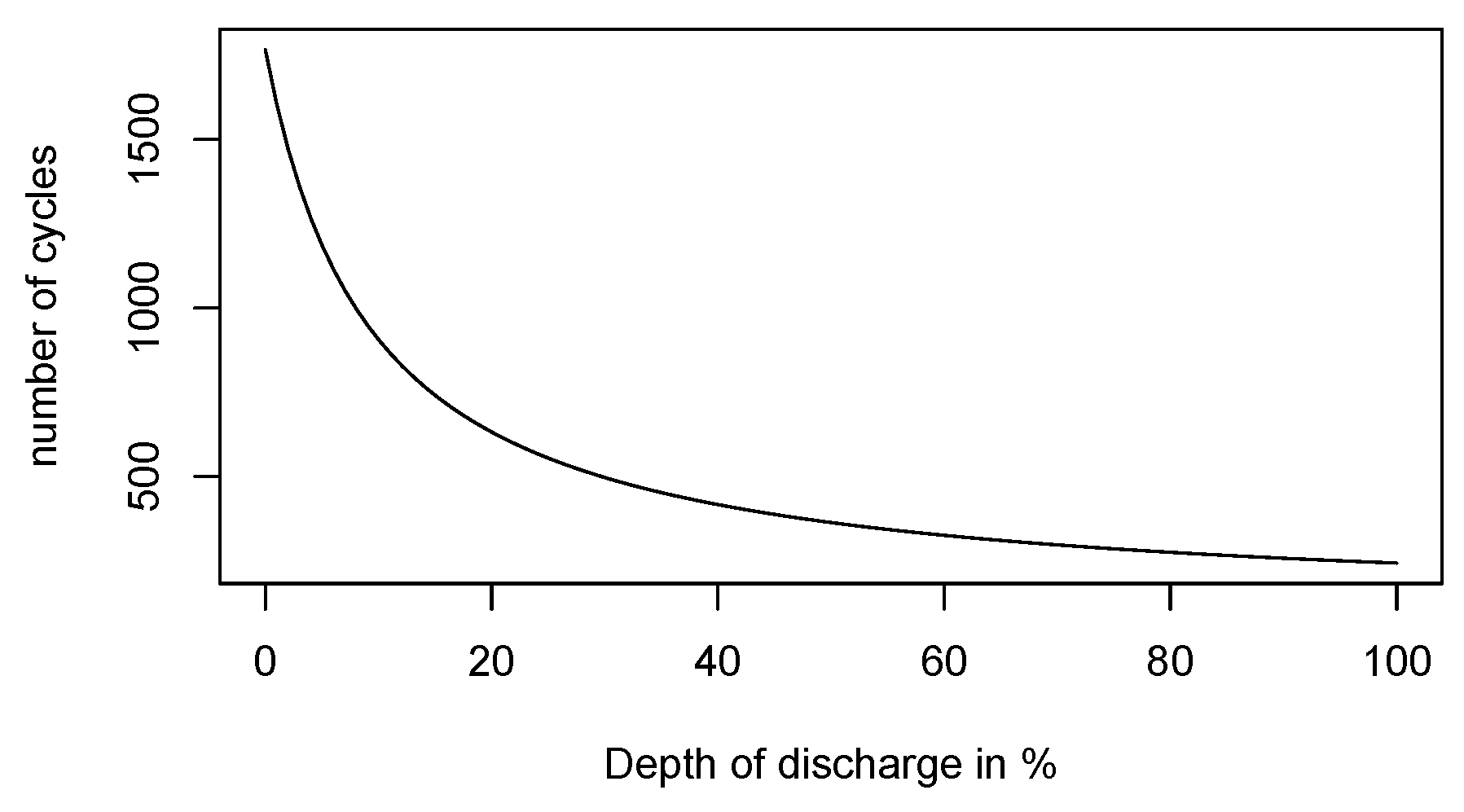The conditions under which batteries are operated affect their performance in terms of the so-called cycle life, which can be defined as the number of cycles completed before the effective battery capacity falls below than $60\%$ of its nominal capacity. Therefore, the Depth of Discharge (DoD) is essential. To give the reader a quantitative understanding of this phenomena, let us consider an example of a lithium ion battery. Assuming that each charge/discharge cycle causes a battery deterioration, one would assume that emptying completely a battery (which corresponds to $100\%$ DoD) 200 times is roughly equivalent (in terms of performance decline) to 400 cycles at $50\%$ DoD and 600 cycles at $33\%$ DoD. However, the actual behavior is different. Usually, a lithium-type battery serves longer than 400 cycles at $50\%$ DoD and significantly longer than 600 cycles at $33\%$ DoD, (see [19]) In our model, we suppose that visiting deep discharge states is costly since it affects battery life. For this reason, we suggest including a user-defined function which penalizes deep discharge states accordingly. Figure 1 illustrates its dependence measured in charge cycles and dependence on depth of discharge. We include such effects into our model by a cost penalization of deep discharge states.

Beyond preventing deep discharge, further operational improvements encompass avoiding that the battery is fully charged (by reducing voltage when charging) and diminishing the so-called charge/discharge rate, which stands for the maximal electric flow during charging/discharging.

We assume that the agent attempts to optimally manage an electricity storage by sequential decisions on the amount of energy procured/purchased through the intraday market and on the optimal charge/discharge of batteries. Obviously, these decisions must take into account the current electricity price, market state, storage level, and all costs and technical restrictions.

Consider an energy retailer facing the obligation to satisfy an unknown energy demand of its customers at times $t=0,\dots ,T-1$, while renewable energy sources produce a random electricity amount given a certain battery storage. To manage a potential energy imbalance, appropriate forward positions are taken in advance and decisions are made to drive the battery storage. This is a typical dynamic control problem, since at any time $t=0,\dots ,T$ an action must be chosen (encompassing a simultaneous energy trade and battery control) which immediately causes some costs but also determines a transition to the next system state (future battery level and market conditions). Clearly, one needs to optimally balance the recent costs against those incurred in the future, based on the current situation. The problems of this type are naturally formulated and solved in terms of dynamic programming.

Remark 2.

Please note that we investigate the problem of electricity storage management within an abstract context which is applicable to most of the deregulated electricity markets, possibly with minor adaptation. Namely we consider energy trading on two time scales. The longer-term trading is realized by forwards or futures or by energy delivery contracts, for instance from the day-ahead trading. In practice, these long-term positions are constantly adjusted on a short-term scale using intraday trading or balancing procedures. This two-scale structure is universal and inherent to any deregulated electricity market and we usually observe significant differences between both scales considering their prices, liquidity, and spread.

Consider an agent who serves an energy consumer whose random demand is (partially) covered from a renewable energy generation facility whose energy output is also random. We denote by $D_t$ the cumulative electricity demand of such facility (which stands for demand if $D_t<0$ and surplus if $D_t>0$) for the delivery period t. Assume that the time point $t=0,\dots ,T-1$ corresponds to the beginning of the period t and agree that the demand $D_t$ is observed after t, at the end of the delivery period t. Let us agree to model $D_t=d_t+{\epsilon }_t$, with a zero-mean random variable ${\epsilon }_t$ standing for the deviation of the realized demand $D_t$ from its prediction $d_t$, which is observable at time t. Moreover, assume that at each time $t=0,\dots ,T$, the producer can take a forward position which attempts to cover $D_t$. Let us describe such position as $d_t+f_t$ where $f_t$ stands for the deviation of the total amount traded forward from the prediction $d_t$. In generic situations, the quantity $f_t$ can be considered to be a “safety margin” which must be purchased on the top of predicted demand $d_t$ to avoid a potential energy shortage during delivery interval. However, we do not assume that $f_t$ or $d_t$ must always be positive. Moreover, introduce the control variable $b_t$, standing for the decision to transfer the energy amount $|b_t|$ from/to the battery, where $b_t>0$ and $b_t<0$ represent discharging and charging actions, respectively. Here, we agree that these control actions must be decided at time t (immediately before the delivery period t starts). With these assumptions, the energy to be balanced during delivery period $t=0,\dots ,T$ using electricity grid is

$$\begin{array}{c}\hfill f_t+d_t-D_t+b_t=f_t+b_t-{\epsilon }_t.\end{array}$$

(28)

Please note that on the right-hand side of this equation, the quantities $f_t$ and $b_t$ must be chosen at t whereas ${\epsilon }_t$ becomes observable after time t.

Now we turn to storage control costs and introduce electricity prices

$$\begin{array}{c}\hfill {\Psi }_t=({\Psi }_t^{+},{\Psi }_t^0,{\Psi }_t^{-})t=0,\dots ,T,\end{array}$$

(29)

with the interpretation that for delivery period t, ${\Psi }_t^0$ stands for the forward price, whereas ${\Psi }_t^{+}$ and ${\Psi }_t^{-}$ are the so-called upper and the lower balancing prices.

Remark 3.

Please note that ${\Psi }_t^0$ stands for the price of energy from long-term market. In the sense of the above remark, this price can represent a forward, futures, or day-ahead price of electrical energy in front of delivery, depending on modeling.

While the forward price ${\Psi }_t^0$ is listed prior to the delivery period t and applies to energy traded in advance, the balancing prices ${\Psi }_t^{+}$, ${\Psi }_t^{-}$ are determined during delivery period t and apply for purchase and procurement of the grid energy. Usually, it holds that

$$\begin{array}{c}\hfill 0\le {\Psi }_t^{+}<{\Psi }_t^0<{\Psi }_t^{-}t=0,\dots ,T.\end{array}$$

(30)

In practice, the price range $[{\Psi }_t^{+},{\Psi }_t^{-}]$ can be wide, meaning that ${\Psi }_t^{+}$ is significantly lower than ${\Psi }_t^0$ which is lower than ${\Psi }_t^{-}$. This issue makes any balancing using grid energy potentially unfavorable. For this reason, the agent attempts to meet the demand as precisely as possible using a combination of the energy from the forward position and from the battery. More specifically, we suppose that the costs, associated with taking forward position, are given by

$$\begin{array}{c}\hfill {\Psi }_t^0(d_t+f_t)+q{(d_t+f_t)}^2\end{array}$$

(31)

where $q>0$ is a coefficient, representing the elasticity of the forward price with respect to contract volume. The total costs associated with energy balancing during the period $t=0,\dots ,T$ is given by

$$\begin{array}{c}\hfill {\Psi }_t^0(d_t+f_t)+q{(d_t+f_t)}^2-{\Psi }_t^{+}{(f_t+b_t-{\epsilon }_t)}^{+}+{\Psi }_t^{-}{(f_t+b_t-{\epsilon }_t)}^{-}.\end{array}$$

(32)

Please note that this quantity is observable after t and is controlled by the variables $f_t$ and $b_t$ which must be chosen at t.

Let us precisely formulate the assumptions on random variables observables, concerning the time of their observation. Suppose that the processes ${\left(d_t\right)}_{t=0}^T$ ${\left(f_t\right)}_{t=0}^T$, ${\left(b_t\right)}_{t=0}^T$, ${\left({\epsilon }_t\right)}_{t=0}^T$ are given on a filtered probability space $(\Omega ,\mathcal{F},\mathbb{P},{\left({\mathcal{F}}_t\right)}_{t=0}^{T+1})$ where ${\mathcal{F}}_t$ represents the information available at time point t, just before the start of the delivery period t. According to the above modeling, we suppose that for $t=0,\dots ,T$

$$\begin{array}{c}{d}_t,f_t,b_t,{\Psi }_t^0\mathrm{are}{\mathcal{F}}_t-\mathrm{measurable},\mathrm{and}\\ {\epsilon }_t,{\Psi }_t^{+},{\Psi }_t^{-}\mathrm{are}{\mathcal{F}}_{t+1}-\mathrm{measurable}.\end{array}$$

Let us suppose that

$$\begin{array}{c}{\Psi }_t=({\Psi }_t^{-},{\Psi }_t^0,{\Psi }_t^{+})\mathrm{and}{\epsilon }_t\mathrm{are}\\ \mathrm{conditionally}\mathrm{independent},\mathrm{given}{\mathcal{F}}_t\end{array}t=0,\dots ,T,$$

(33)

and denote by ${\mathbb{E}}_t(·)$ the expectation, conditioned on ${\mathcal{F}}_t$ for $t=0,\dots ,T$. Applying such conditional expectation ${\mathbb{E}}_t(·)$ to (32), we use the conditional independence (4) to obtain

$$\begin{array}{c}\hfill {\overline{\Psi }}_t^0(d_t+f_t)+q{(d_t+f_t)}^2-{\overline{\Psi }}_t^{+}{\mathbb{E}}_t\left[{(f_t+b_t-{\epsilon }_t)}^{+}\right]+{\overline{\Psi }}_t^{-}{\mathbb{E}}_t\left[{(f_t+b_t-{\epsilon }_t)}^{-}\right].\end{array}$$

(34)

In this equation, the prices expected in front of delivery, are denoted by

$${\overline{\Psi }}_t^{-}={\mathbb{E}}_t\left({\Psi }_t^{-}\right),{\overline{\Psi }}_t^0={\Psi }_t^0={\mathbb{E}}_t\left({\Psi }_t^0\right),{\overline{\Psi }}_t^{+}={\mathbb{E}}_t\left({\Psi }_t^{+}\right),t=0,\dots ,T.$$

To simplify our energy storage management, we furtherer agree that the distribution of prediction errors does not depend on recent information in the sense that

$${\epsilon }_t\mathrm{and}{\mathcal{F}}_t\mathrm{are}\mathrm{independent},t=0,\dots ,T.$$

(35)

This natural assumption yields a compact form for the expected costs (34):

$${\overline{\Psi }}_t^0(d_t+f_t)+q{(d_t+f_t)}^2-{\overline{\Psi }}_t^{+}{h}_t^{+}(f_t+b_t)+{\overline{\Psi }}_t^{-}{h}_t^{-}(f_t+b_t)$$

(36)

with functions $h^{+}$ and $h^{-}$ explicitly computable from

$$h_t^{+}\left(u\right)=\mathbb{E}\left[{(u-{\epsilon }_t)}^{+}\right],h_t^{-}\left(u\right)=\mathbb{E}\left[{(u-{\epsilon }_t)}^{-}\right],u\in \mathbb{R},t=0,\dots ,T.$$

(37)

In view of (34)–(37), the expected costs of (32) depend on the energy control variables f and b as

$$(f,b)\mapsto {\overline{\Psi }}_t^0(d_t+f)+q{(d_t+f)}^2-{\overline{\Psi }}_t^{+}{h}_t^{+}(f+b)+{\overline{\Psi }}_t^{-}{h}_t^{-}(f+b)$$

(38)

Please note that these costs are expected at time t and can be changed by appropriate adjustment of decision variables $f,b\in \mathbb{R}$.

For an agent concerned with the minimization of all costs accumulated within the decision period ranging from $t=0$ to $t=T$, the dynamical aspects are important. Specifically, the decision at time t to use energy b from the storage changes the storage level, which has a distinct impact on the availability of energy in the future, influencing all following decisions.

To formulate our storage control as a dynamic programming problem, we assume that a Markov dynamics ${\left(Z_t\right)}_{t=0}^T$ on $(\Omega ,\mathcal{F},\mathbb{P},{\left({\mathcal{F}}_t\right)}_{t=0}^T)$ carries all relevant information. Therefore, we suppose that ${\left(Z_t\right)}_{t=0}^T$ is a Markovian process which takes values in ${\mathbb{R}}^d$. This process describes the evolution of all relevant state variables of the environment. In particular, we assume that the expected prices are represented by function $\psi :{\mathbb{R}}^d\to {\mathbb{R}}^3$ of state variables, whose components $\psi =({\psi }_t^{-},{\psi }_t^0,{\psi }_t^{+})$ determine the prices as follows:

$$({\overline{\Psi }}_t^{-},{\overline{\Psi }}_t^0,{\overline{\Psi }}_t^{+})={\psi }_t\left(Z_t\right)=({\psi }_t^{-}\left(Z_t\right),{\psi }_t^0\left(Z_t\right),{\psi }_t^{+}\left(Z_t\right))t=0,\dots ,T.$$

(39)

In accordance to (30), we require for $t=0,\dots ,T$ that

$$\begin{array}{c}\hfill 0\le {\psi }_t^{+}\left(z\right)<{\psi }_t^0\left(z\right)<{\psi }_t^{-}\left(z\right),z\in {\mathbb{R}}^d.\end{array}$$

(40)

Furthermore, we suppose that at any time $t=0,\dots ,T$, the conditional expectation of the next period’s demand is described in terms of a deterministic function

$$d:\{0,\dots ,T\}\times {\mathbb{R}}^d\to \mathbb{R},(t,z)\mapsto d_t\left(z\right).$$

Besides the state of the environment $z\in {\mathbb{R}}^d$, the other important state variable is the current storage level $e\in I$. Having denoted the minimal and the maximal energy amounts of the battery by $\underline{e}$ and $\overline{e}$ respectively, we suppose that the storage level e represents by the amount e of energy, which is needed to fully charge the battery. With this interpretation, our variable is the

$$\begin{array}{c}\hfill \mathrm{resource}\mathrm{level}e,\mathrm{which}\mathrm{takes}\mathrm{values}\mathrm{in}\mathrm{the}\mathrm{interval}I=]0,\overline{e}-\underline{e}[.\end{array}$$

(41)

In view of (34)–(39), the expected costs of (32) are now written in terms of a function

$$\begin{array}{cc}\hfill C_t^{e,z}(f,b)=& {\psi }_t^0\left(z\right)(d_t\left(z\right)+f)+q{(d_t\left(z\right)+f)}^2-{\psi }_t^{+}\left(z\right)h_t^{+}(f+b)\hfill \\ \hfill & +{\psi }_t^{-}\left(z\right)h_t^{-}(f+b)+\chi \left(e\right)\hfill \end{array}$$

(42)

of the resource level $e\in I$, the state variable $z\in {\mathbb{R}}^d$, and the control variables $f,b\in \mathbb{R}$ for $t=0,\dots ,T$. Please note that in (42) we include the costs $\chi \left(e\right)$ of deep discharge corresponding to the resource level $e\in I$, modeled by an

$$\begin{array}{c}\hfill \mathrm{increasing}\mathrm{and}\mathrm{convex}\mathrm{function}\chi :I\to \mathbb{R}.\end{array}$$

(43)

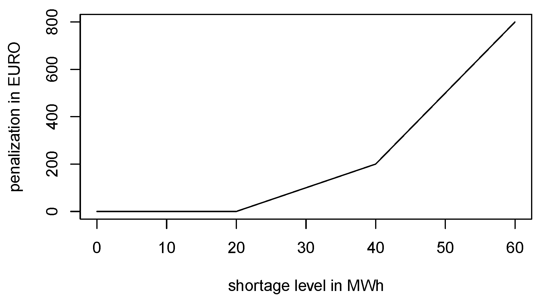
Remark 4.

Ideally, an understanding of the chemistry of a particular battery will suggest some generic penalization function. However, in practice, there are diverse approaches to assess (in economic terms) how the battery life is affected by visiting a deep discharge state. Here, the usual cycle life graph (as in Figure 1), does not detail all aspects required by our approach. The point is that the cycle life is determined by charge/discharge periods oscillating linearly between the minimal and the maximal capacity, rather by a certain strategy run within a random environment. Such life cycle diagrams do not provide any information whether it could be worth visiting a deep discharge state for a short period of time in order to catch an electricity price spike. Given diverse battery storage technologies, there is no simple way of determining an appropriate penalization function. For this reason, the authors suggest a pragmatic approach: For a pre-specified penalization as depicted in Figure 2, the user will calculate the corresponding optimal strategy which must be examined and assessed in simulations. If required by simulation results, the penalty function can be altered, followed by another round of optimization and simulations. Such attempts can be repeated until satisfactory results (considering battery life expectation, peak load response, and total revenue) are reached.

Now, let us propose Bellman recursion for our battery control problem. Recall that in our modeling, the state variables at time $t=0,\dots ,T$ comprise a market situation described by the realization $z=Z_t$ of the environment state process and the current resource level $e\in I$. Having supposed that at the final date $t=T$, in the environment state $z=Z_T$ the entire battery storage content $\overline{e}-e$ can be sold at the market price ${\psi }_T^0\left(z\right)$, we agree that the terminal costs function is

$$C_T(e,z)=-{\psi }_T^0\left(z\right)(\overline{e}-\underline{e}-e)(z,e)\in {\mathbb{R}}^d\times I.$$

(44)

This quantity determines the value function $V_T$ at the final time T by

$$V_T(e,z)=C_T(e,z),(z,e)\in {\mathbb{R}}^d\times I.$$

(45)

Prior to the terminal time $t=0,\dots ,T-1$, the backward induction yields the value functions ${\left(V_t\right)}_{t=0}^{T-1}$ recursively by

$$\begin{array}{cc}\hfill & {\tilde{V}}_{t+1}(e,z)=\mathbb{E}\left(V(Z_{t+1},e)\right|Z_t=z)(z,e)\in {\mathbb{R}}^d\times I,\hfill \end{array}$$

(46)

$$\begin{array}{cc}\hfill & V_t(e,z)=\underset{(f,b)\in \Xi (e,z)}{min}\left(C_t^{e,z}(f,b)+{\tilde{V}}_{t+1}(e+b,z)\right)(z,e)\in {\mathbb{R}}^d\times I,\hfill \end{array}$$

(47)

where the minimum must be taken over the set $\Xi (e,z)$ of all admissible controls

$$\Xi (e,z)=\left\{\right(f,b):f,b\in \mathbb{R},e+b\in I\},e\in I$$

(48)

due to restriction that the energy transfer from/to the storage is limited by the storage capacity. However, in our approach, many arguments rely on the assumption that the set of admissible decisions does not depend on the current situation. To replace the minimization over admissible controls $\Xi (e,z)$ in (11) by a minimization over an unrestricted set

$$\Xi =\left\{\right(f,b):f,b\in \mathbb{R}\},$$

we introduce a penalization for violation $(f,b)\notin \Xi (e,z)$, having in mind that for a sufficiently strong penalization it will be never optimal to violate the restriction $e+b\in I$. This concept is realized by the following recursions:

$$\begin{array}{cc}\hfill & V_T(e,z)=C_T(e,z),(z,e)\in {\mathbb{R}}^d\times I\hfill \end{array}$$

(49)

$$\begin{array}{cc}\hfill & {\tilde{V}}_{t+1}(e,z)=\left\{\begin{array}{cc}\mathbb{E}\left(V_{t+1}(e,Z_{t+1})\right|Z_t=z)\hfill & e\in I\hfill \\ +\infty \hfill & e\notin I\hfill \end{array}\right.,z\in {\mathbb{R}}^d\hfill \end{array}$$

(50)

$$\begin{array}{cc}\hfill & V_t(e,z)=\underset{(f,b)\in \Xi }{inf}\left(C_t^{e,z}(f,b)+{\tilde{V}}_{t+1}(e+b,z)\right),(z,e)\in {\mathbb{R}}^d\times I.\hfill \end{array}$$

(51)

Please note that with this definition, the functions ${\left(V_t\right)}_{t=0}^T$ satisfy (45)–(48) if and only if they fulfill (49)–(51).

5. Variables Reduction for Battery Control

In this section, we adopt and use our variable reduction technique to the specific situation described in Section 4. Therefore, we show that all assumptions of Theorem 1 are fulfilled. Recall from our modeling (44), (42) that the set of activities is given by

$$\begin{array}{c}\hfill \Xi =\left\{\right(f,b):f\in \mathbb{R},b\in \mathbb{R}\}\end{array}$$

(52)

with the interpretation that f and b represent the energy from trading and that from the battery, respectively. On this account, we have assumed that the costs and resource consumption functions are given by

$$\begin{array}{cc}\hfill C_t^{e,z}(f,b)=& {\psi }_t^0\left(z\right)(d_t\left(z\right)+f)+q{(d_t\left(z\right)+f)}^2-{\psi }_t^{+}\left(z\right)h_t^{+}(f+b)\hfill \end{array}$$

$$\begin{array}{cc}\hfill & +{\psi }_t^{-}\left(z\right)h_t^{-}(f+b)+\chi \left(e\right)\hfill \end{array}$$

(53)

$$\begin{array}{cc}\hfill E_t^{e,z}(f,b)=& b\mathrm{for}z\in {\mathbb{R}}^d,(f,b)\in \Xi ,t=0,\dots ,T-1.\hfill \end{array}$$

(54)

Here the coefficient $q>0$ represents the price elasticity whereas the functions $h_t^{+}$ and $h_t^{-}$ are defined by (37) as

$$\begin{array}{cc}\hfill h_t^{+}\left(u\right)& =\mathbb{E}\left[{(u-{\epsilon }_t)}^{+}\right]={\int }_{\mathbb{R}}{(u-ϵ)}^{+}{\mathbb{P}}_{{\epsilon }_t}\left(dϵ\right),\hfill \\ \hfill h_t^{-}\left(u\right)& =\mathbb{E}\left[{(u-{\epsilon }_t)}^{-}\right]={\int }_{\mathbb{R}}{(u-ϵ)}^{-}{\mathbb{P}}_{{\epsilon }_t}\left(dϵ\right),\hfill \end{array}$$

in terms of the distribution ${\mathbb{P}}_{{\epsilon }_t}$ of the demand prediction error ${\epsilon }_t$, this distribution is non-random by assumption (35). Define the function

$$\begin{array}{c}{h}_t(z,u)={\int }_{\mathbb{R}}[-{\psi }_t^{+}\left(z\right){(u-ϵ)}^{+}+{\psi }_t^{-}\left(z\right){(u-ϵ)}^{-}]{\mathbb{P}}_{{\epsilon }_t}\left(dϵ\right)\end{array}z\in {\mathbb{R}}^d,u\in \mathbb{R}$$

(55)

and observe that

$$\begin{array}{c}\hfill u\mapsto h_t(z,u)\mathrm{is}\mathrm{convex}\mathrm{and}\mathrm{non}-\mathrm{increasing}\mathrm{on}\mathbb{R}\mathrm{for}\mathrm{each}z\in {\mathbb{R}}^d\end{array}$$

(56)

due to $0\le {\psi }_t^{+}\left(z\right)<{\psi }_t^{-}\left(z\right)$ stated in (30). Using (55), we rewrite (53) as

$$\begin{array}{c}\hfill \begin{array}{c}{C}_t^{e,z}(f,b)={\psi }_t^0\left(z\right)(d_t\left(z\right)+f)+q{(d_t\left(z\right)+f)}^2+h_t(z,f+b)+\chi \left(e\right)\\ \mathrm{for}(f,b)\in \Xi ,(e,z)\in I\times {\mathbb{R}}^d.\end{array}\end{array}$$

(57)

With this representation, the convexity required by (24) is obvious, since the functions $(f,b)\mapsto q{(d_t\left(z\right)+f)}^2$ and $(f,b)\mapsto h_t(z,f+b)$ are convex on $\Xi$, while $e\mapsto \chi \left(e\right)$ is convex on I.

To verify (22), consider ${\xi }^{\prime }=(f^{\prime },b^{\prime })\in \Xi$ and $e,e^{\prime }\in I$ with $e<e^{\prime }$ to define

$$\xi =(f,b)=(f^{\prime },b^{\prime }+e^{\prime }-e)$$

which yields the same resource consumption

$$e+E_t^{e,z}\left(\xi \right)=e^{\prime }+b^{\prime }=e^{\prime }+E_t^{e^{\prime },z}\left({\xi }^{\prime }\right)$$

at no greater costs

$$\begin{array}{cc}\hfill C_t^{e,z}\left(\xi \right)& ={\psi }_t^0\left(z\right)(d_t\left(z\right)+f^{\prime })+q{(d_t+f^{\prime })}^2+h_t(z,f^{\prime }+b^{\prime }+e^{\prime }-e)+\chi \left(e\right)\hfill \\ \hfill & \le {\psi }_t^0\left(z\right)(d_t\left(z\right)+f^{\prime })+q{(d_t+f^{\prime })}^2+h_t(z,f^{\prime }+b^{\prime })+\chi \left(e^{\prime }\right)=C_t^{e^{\prime },z}\left({\xi }^{\prime }\right),\hfill \end{array}$$

since $h_t$ is non-increasing by (56) in the second variable and the deep discharge penalization function $\chi$ is strictly increasing by assumption (43).

Now let us turn to the Legendre-type transform and verify (21) and (23). To obtain explicit expressions, let us suppose for the sake of concreteness that

$$\begin{array}{c}\mathrm{for}t=0,\dots ,T-1,\mathrm{the}\mathrm{distribution}{\mathbb{P}}_{{\epsilon }_t}\mathrm{possesses}\mathrm{a}\mathrm{strictly}\\ \mathrm{increasing}\mathrm{and}\mathrm{continuous}\mathrm{distribution}\mathrm{function}{F}_{{\epsilon }_t}.\end{array}$$

(58)

The derivative of the function $h_t$ from (55) under the assumptions (58) is evaluated explicitly as

$$\begin{array}{c}\hfill {\partial }_{(0,1)}{h}_t(z,u)=({\psi }_t^{-}\left(z\right)-{\psi }_t^{+}\left(z\right))F_{{\epsilon }_t}\left(u\right)-{\psi }_t^{-}\left(z\right),u\in \mathbb{R}.\end{array}$$

(59)

Given an $A\in \mathbb{R}$, consider the minimization (12) of $C_t^{e,z}\left(\xi \right)+A{E}_t^{e,z}\left(\xi \right)$ over $\xi \in \Xi$, which yields the minimization of a convex and smooth function

$${\mathbb{R}}^2\to \mathbb{R},(f,b)\mapsto {\psi }_t^0\left(z\right)(d_t\left(z\right)+f^{\prime })+q{(d_t\left(z\right)+f^{\prime })}^2+h_t(z,f+b)+Ab$$

(60)

whose first-order conditions are

$${\psi }_t^0\left(z\right)+2q(d_t\left(z\right)+f)+{\partial }_{(0,1)}{h}_t(z,f+b)=0,{\partial }_{(0,1)}{h}_t(z,f+b)+A=0.$$

These conditions are fulfilled by $(f^{\ast },b^{\ast })\in {\mathbb{R}}^2$ obtained from

$${\psi }_t^0\left(z\right)+2q(d_t\left(z\right)+f^{\ast })=A,{\partial }_{(0,1)}{h}_t(z,f^{\ast }+b^{\ast })=-A.$$

(61)

That is, the unique minimum of (60) exists for $0<{\psi }_t^{+}\left(z\right)<A<{\psi }_t^{-}\left(z\right)$ and is given by solution to (61) as

$$\begin{array}{cc}\hfill f_t^{e,z}\left(A\right)& =\frac{A-{\psi }_t^0\left(z\right)}{2q}-d_t\left(z\right),\hfill \end{array}$$

(62)

$$\begin{array}{cc}\hfill b_t^{e,z}\left(A\right)& =F_{{\epsilon }_t}^{-1}\left(\frac{{\psi }_t^{-}\left(z\right)-A}{{\psi }_t^{-}\left(z\right)-{\psi }_t^{+}\left(z\right)}\right)-\frac{A-{\psi }_t^0\left(z\right)}{2q}+d_t\left(z\right),\hfill \end{array}$$

(63)

giving the minimizer

$${\mathcal{X}}_t^{e,z}\left(A\right)=(f_t^{e,z}\left(A\right),b_t^{e,z}\left(A\right))$$

for (21) over the relevant interval

$$\begin{array}{c}\hfill A\in {\mathcal{A}}^{e,z}=]{\psi }_t^{+}\left(z\right),{\psi }_t^{-}\left(z\right)[.\end{array}$$

(64)

Furthermore, assumption (23) is satisfied, since

$$A\mapsto E_t^{e,z}\left({\mathcal{X}}_t^{e,z}\left(A\right)\right)=b_t^{e,z}\left(A\right)$$

is linearly decreasing over the interval (64) ranging from a positive

$$\begin{array}{cc}\hfill \underset{A\downarrow {\psi }_t^{+}\left(z\right)}{lim}{b}_t^{e,z}\left(A\right)& =F_{{\epsilon }_t}^{-1}\left(1_{-}\right)-\frac{{\psi }_t^{+}\left(z\right)-{\psi }_t^0\left(z\right)}{2q}>0,\hfill \end{array}$$

to a negative value

$$\begin{array}{cc}\hfill \underset{A\uparrow {\psi }_t^{+}\left(z\right)}{lim}{b}_t^{e,z}\left(A\right)& =F_{{\epsilon }_t}^{-1}\left(0_{+}\right)-\frac{{\psi }_t^{-}\left(z\right)-{\psi }_t^0\left(z\right)}{2q}<0.\hfill \end{array}$$

All ingredients required for (14)–(16) are specified for $t=0,\dots ,T-1$, $z\in {\mathbb{R}}^d$, $A\in {\mathcal{A}}^{e,z}$ by the following quantities

$$\begin{array}{cc}\hfill E_t^{e,z}\left({\mathcal{X}}_t^{e,z}\left(A\right)\right)& =b_t^{e,z}\left(A\right)\hfill \\ \hfill C_t^{e,z}\left({\mathcal{X}}_t^{e,z}\left(A\right)\right)& ={\psi }_t^0\left(z\right)(d_t\left(z\right)+f_t^{e,z})\left(A\right)+q(d_t\left(z\right)+f_t^{e,z})A^2+h_t(z,f_t^{e,z}\left(A\right)+b_t^{e,z}\left(A\right))+\chi \left(e\right)\hfill \end{array}$$

which are relevant in (14)–(16).

6. The Variables Reduction Technique

This section is devoted to the derivation of Theorem 1. Let us prepare the proof by gradually showing auxiliary results. Our arguments rely on convexity of the functions ${\left(V_t\right)}_{t=0}^T$ from (9)–(11). It turns out that, based on the assumption

$$\begin{array}{c}\hfill \begin{array}{c}{\tilde{V}}_{t+1}(·,z)\mathrm{is}\mathrm{convex}\mathrm{and}\mathrm{non}-\mathrm{decreasing}\mathrm{on}I\\ \mathrm{and}{\tilde{V}}_{t+1}(·,z)=+\infty \mathrm{on}\mathbb{R}\setminus I,\mathrm{for}\mathrm{all}z\in {\mathbb{R}}^d,\end{array}\end{array}$$

(65)

the same properties can be deduced for ${\tilde{V}}_t(·,z)$ as formulated in the following lemma.

Lemma 1.

Given costs and resource consumption (18), let $t\in \{0,\dots ,T-1\}$, suppose that (65) holds and consider $V_t(·,z)$ defined by (11). If (22) holds then $V_t(·,z)$ is non-decreasing on I for all $z\in {\mathbb{R}}^d$. If in addition (24) is satisfied, then $V_t(·,z)$ is non-decreasing and convex on I for all $z\in {\mathbb{R}}^d$.

Proof. 

Given $z\in {\mathbb{R}}^d$, $e,e^{\prime }\in I$ with $e<e^{\prime }$, and arbitrary ${\xi }^{\prime }\in \Xi$ there exists by (22) an action $\xi \in \Xi$ with

$$e+E_t^{e,z}\left(\xi \right)=e^{\prime }+E_t^{e^{\prime },z}\left({\xi }^{\prime }\right)\mathrm{and}{C}_t^{e,z}\left(\xi \right)\le C_t^{e^{\prime },z}\left({\xi }^{\prime }\right)$$

which gives

$$C_t^{e,z}\left(\xi \right)+{\tilde{V}}_{t+1}(e+E_t^{e,z}\left(\xi \right),z)\le C_t^{e^{\prime },z}\left({\xi }^{\prime }\right)+{\tilde{V}}_{t+1}(e^{\prime }+E_t^{e^{\prime },z}\left({\xi }^{\prime }\right),z)$$

and shows $V_t(e,z)\le V_t(e^{\prime },z)$ by minimization in $\xi$ and ${\xi }^{\prime }$ over $\Xi$.

Now we turn to the convexity. Using the infimum in (11) for each $\delta >0$, there exist $\xi ,{\xi }^{\prime }\in \Xi$ such that

$$\begin{array}{cc}\hfill \frac{\delta }{2}+V_t(e,z)& \ge C_t^{e,z}\left(\xi \right)+{\tilde{V}}_{t+1}(e+E_t^{e,z}\left(\xi \right),z),\hfill \\ \hfill \frac{\delta }{2}+V_t(e^{\prime },z)& \ge C_t^{e^{\prime },z}\left({\xi }^{\prime }\right)+{\tilde{V}}_{t+1}(e^{\prime }+E_t^{e^{\prime },z}\left({\xi }^{\prime }\right),z).\hfill \end{array}$$

Please note that these values are finite due to (20), which means that

$$e+E_t^{e,z}\left(\xi \right)\in I,e^{\prime }+E_t^{e^{\prime },z}\left({\xi }^{\prime }\right)\in I.$$

That is, by convex linear combinations of the activities ($\Xi$ is convex by (24)) and resource levels we obtain

$$\begin{array}{cc}\hfill {\xi }^{\left(\lambda \right)}& =\lambda \xi +(1-\lambda ){\xi }^{\prime }\in \Xi \hfill \\ \hfill e^{\left(\lambda \right)}& =\lambda e+(1-\lambda )e^{\prime }\in I.\hfill \end{array}$$

Now, by convexity of costs functions (24) it holds that

$$\begin{array}{cc}\hfill \lambda C_t^{e,z}\left(\xi \right)+(1-\lambda )C_t^{e^{\prime },z}\left({\xi }^{\prime }\right)& \ge C_t^{e^{\left(\lambda \right)},z}\left({\xi }^{\left(\lambda \right)}\right)\hfill \end{array}$$

and using assumption (65) we conclude

$$\begin{array}{c}\hfill \lambda {\tilde{V}}_{t+1}(e+E_t^{e,z}\left(\xi \right),z)+(1-\lambda ){\tilde{V}}_{t+1}(e^{\prime }+E_t^{e^{\prime },z}\left({\xi }^{\prime }\right),z)\ge \\ \hfill \ge {\tilde{V}}_{t+1}(\lambda e+(1-\lambda )e^{\prime }+\lambda E_t^{e,z}\left(\xi \right)+(1-\lambda )E_t^{e^{\prime },z}\left({\xi }^{\prime }\right),z)\ge \\ \hfill \ge {\tilde{V}}_{t+1}(e^{\left(\lambda \right)}+E_t^{e^{\left(\lambda \right)},z}\left({\xi }^{\left(\lambda \right)}\right),z).\end{array}$$

From this, we proceed with

$$\begin{array}{cc}\hfill \delta +\lambda V_t(e,z)+(1-\lambda )V_t(e^{\prime },z)& \ge C_t^{e^{\left(\lambda \right)},z}\left({\xi }^{\left(\lambda \right)}\right)+{\tilde{V}}_{t+1}(e^{\left(\lambda \right)}+E_t^{e^{\left(\lambda \right)},z}\left({\xi }^{\left(\lambda \right)}\right),z)\hfill \\ \hfill & \ge \underset{\xi \in \Xi }{inf}\left(C_t^{e^{\left(\lambda \right)},z}\left(\xi \right)+{\tilde{V}}_{t+1}(e^{\left(\lambda \right)}+E_t^{e,z}\left(\xi \right),z)\right)\hfill \\ \hfill & \ge V_t(e^{\left(\lambda \right)},z)\hfill \end{array}$$

that shows the desired convexity. □

In what follows, we recall the notion $\nabla g$ of the so-called sub-gradient of a convex function $g:{\mathbb{R}}^n\to \mathbb{R}\cup \{\infty \}$, ($n\in \mathbb{N}$) which is defined at each point $u\in {\mathbb{R}}^n$ as the family of linear functionals

$$\nabla g\left(u\right)=\{l:{\mathbb{R}}^n\to \mathbb{R}:l\mathrm{is}\mathrm{linear}\mathrm{with}g\left(u\right)+l(u^{\prime }-u)\le g\left(u^{\prime }\right),\mathrm{for}{u}^{\prime }\in {\mathbb{R}}^n\}.$$

For a function V on $I\times {\mathbb{R}}^d\to \mathbb{R}$ as in (65) which is convex in the first component on I, we agree to consider its sub-gradient in the first component, only for arguments in I. More precisely, for $(e,z)\in I\times {\mathbb{R}}^d$ we write $\nabla V(e,z)$ to denote the set of linear functionals $l:\mathbb{R}\to \mathbb{R}$ satisfying

$$V(e,z)+l(e^{\prime }-e)\le V(e^{\prime },z)\mathrm{for}\mathrm{all}{e}^{\prime }\in \mathbb{R}.$$

Now, let us elaborate on the fixed-point property of the virtual resource price in the optimal regime in the spirit of the remark before Section 4.

Lemma 2.

Assume that the costs and resource consumption functions are given as in (18). Let $t\in \{0,\dots ,T-1\}$ and ${\tilde{V}}_{t+1}$ be a function which satisfies (65), furthermore, suppose that (21) holds. If for $(e,z)\in {\mathbb{R}}^d$ there exists $A^{\ast }\in {\mathcal{A}}^{e,z}$ satisfying the fixed-point equation

$$\begin{array}{c}\hfill A^{\ast }\in \nabla {\tilde{V}}_{t+1}(e+E_t^{e,z}\left({\mathcal{X}}_t^{e,z}\left(A^{\ast }\right)\right),z),\end{array}$$

(66)

then ${\xi }^{\ast }={\mathcal{X}}_t^{e,z}\left(A^{\ast }\right)$ is a minimizer to (11).

Proof. 

By assumption (21) the minimizer ${\xi }^{\ast }={\mathcal{X}}_t^{e,z}\left(A^{\ast }\right)$ to (12) satisfies

$$\begin{array}{c}\hfill C_t^{e,z}\left({\xi }^{\ast }\right)+A^{\ast }{E}_t^{e,z}\left({\xi }^{\ast }\right)\le C_t^{e,z}\left(\xi \right)+A^{\ast }{E}_t^{e,z}\left(\xi \right)\end{array}$$

(67)

for each $\xi \in \Xi$, which is equivalent to

$$\begin{array}{c}\hfill C_t^{e,z}\left({\xi }^{\ast }\right)-C_t^{e,z}\left(\xi \right)\le A^{\ast }(E_t^{e,z}\left(\xi \right)-E_t^{e,z}\left({\xi }^{\ast }\right)).\end{array}$$

(68)

On the other hand, since $A^{\ast }\in \nabla {\tilde{V}}_{t+1}(e+E_t^{e,z}\left({\xi }^{\ast }\right),z)$ by assumption (66), we conclude that

$$\begin{array}{c}\hfill A^{\ast }(E_t^{e,z}\left(\xi \right)-E_t^{e,z}\left({\xi }^{\ast }\right))\le {\tilde{V}}_{t+1}(e+E_t^{e,z}\left(\xi \right),z)-{\tilde{V}}_{t+1}(e+E_t^{e,z}\left({\xi }^{\ast }\right),z).\end{array}$$

(69)

By combining (68) and (69)

$$C_t^{e,z}\left({\xi }^{\ast }\right)-C_t^{e,z}\left(\xi \right)\le {\tilde{V}}_{t+1}(e+E_t^{e,z}\left(\xi \right),z)-{\tilde{V}}_{t+1}(e+E_t^{e,z}\left({\xi }^{\ast }\right),z)$$

we obtain the desired assertion

$$C_t^{e,z}\left({\xi }^{\ast }\right)+{\tilde{V}}_{t+1}(e+E_t^{e,z}\left({\xi }^{\ast }\right),z)\le C_t^{e,z}\left(\xi \right)+{\tilde{V}}_{t+1}(e+E_t^{e,z}\left(\xi \right),z).$$

 □

The above lemma suggests determining a minimizer ${\xi }^{\ast }$ to (11) as ${\xi }^{\ast }={\mathcal{X}}_t^{e,z}\left(A^{\ast }\right)$ where $A^{\ast }$ is obtained as a solution to the fixed-point relation (66). However, according to the dynamic programing principle, the virtual resource price $A^{\ast }\in {\mathcal{A}}^{e,z}$ shall be determined by the minimization (27) rather than by solving a fixed-point relation. The result below shows that under natural assumptions, (27) in fact implies (66).

Lemma 3.

Given costs and resource consumption (18), let $t\in \{0,\dots ,T-1\}$ and $(e,z)\in I\times {\mathbb{R}}^d$, suppose that (65) holds and assume that (21) holds and (23) is satisfied. If $A^{\ast }=A^{e,z}$ fulfills (27), then $A^{\ast }$ also fulfills the fixed-point equation (66).

Proof. 

Given $(e,z)\in I\times {\mathbb{R}}^d$, suppose that $A^{\ast }=A^{e,z}\in {\mathcal{A}}^{e,z}$ satisfies (27). Recall that by assumption (23) there exists $A_0\in {\mathcal{A}}^{e,z}$ there exists a root such that $E_t^{e,z}\left({\mathcal{X}}_t^{e,z}\left(A_0\right)\right)=0$. Since this root is included in the minimization, with a finite (due to $e\in I$) value

$$V_{t+1}(e+E_t^{e,z}\left({\mathcal{X}}_t^{e,z}\left(A_0\right)\right),z)=V_{t+1}(z,e)<\infty ,$$

the infimum is also finite

$$C_t^{e,z}\left({\mathcal{X}}_t^{e,z}\left(A^{\ast }\right)\right)+{\tilde{V}}_{t+1}(e+E_t^{e,z}\left({\mathcal{X}}_t^{e,z}\left(A^{\ast }\right)\right),z)<\infty .$$

By the minimum property (27), for each $A\in {\mathcal{A}}^{e,z}$ it holds that

$$\begin{array}{c}\hfill C_t^{e,z}\left({\mathcal{X}}_t^{e,z}\left(A^{\ast }\right)\right)+{\tilde{V}}_{t+1}(e+E_t^{e,z}\left({\mathcal{X}}_t^{e,z}\left(A^{\ast }\right)\right),z)\le \\ \hfill \le C_t^{e,z}\left({\mathcal{X}}_t^{e,z}\left(A\right)\right)+{\tilde{V}}_{t+1}(e+E_t^{e,z}\left({\mathcal{X}}_t^{e,z}\left(A\right)\right),z).\end{array}$$

(70)

Furthermore, by definition of ${\mathcal{X}}_t^{e,z}\left(A\right)$, it holds on the other hand that

$$\begin{array}{c}\hfill C_t^{e,z}\left({\mathcal{X}}_t^{e,z}\left(A\right)\right)+E_t^{e,z}\left({\mathcal{X}}_t^{e,z}\left(A\right)\right)\le C_t^{e,z}\left(\xi \right)+A{E}_t^{e,z}\left(\xi \right)\end{array}$$

for each $\xi \in \Xi$. Replacing $\xi$ by ${\mathcal{X}}_t^{e,z}\left(A^{\ast }\right)$, we deduce

$$\begin{array}{c}\hfill C_t^{e,z}\left({\mathcal{X}}_t^{e,z}\left(A\right)\right)\le C_t^{e,z}\left({\mathcal{X}}_t^{e,z}\left(A^{\ast }\right)\right)+A(E_t^{e,z}\left({\mathcal{X}}_t^{e,z}\left(A^{\ast }\right)\right)-E_t^{e,z}\left({\mathcal{X}}_t^{e,z}\left(A\right)\right))\end{array}$$

which we combine with (70) to obtain

$$\begin{array}{c}\hfill {\tilde{V}}_{t+1}(e+E_t^{e,z}\left({\mathcal{X}}_t^{e,z}\left(A^{\ast }\right)\right),z)\le \\ \hfill \le A(E_t^{e,z}\left({\mathcal{X}}_t^{e,z}\left(A^{\ast }\right)\right)-E_t^{e,z}\left({\mathcal{X}}_t^{e,z}\left(A\right)\right))+{\tilde{V}}_{t+1}(e+E_t^{e,z}\left({\mathcal{X}}_t^{e,z}\left(A\right)\right),z).\end{array}$$

(71)

Introducing for $(ϵ,z)\in I\times {\mathbb{R}}^d$ the notations

$$\begin{array}{cc}\hfill \mathcal{E}\left(A\right)& =e+E_t^{e,z}\left({\mathcal{X}}_t^{e,z}\left(A\right)\right),A\in {\mathcal{A}}^{e,z},\hfill \\ \hfill \tilde{V}\left(ϵ\right)& ={\tilde{V}}_{t+1}(ϵ,z),\hfill \end{array}$$

the inequality (71) is written as

$$\tilde{V}\left(\mathcal{E}\left(A^{\ast }\right)\right)+A(\mathcal{E}\left(A\right)-\mathcal{E}\left(A^{\ast }\right))\le \tilde{V}\left(\mathcal{E}\left(A\right)\right),A\in {\mathcal{A}}^{e,z}.$$

(72)

For a strictly increasing sequence ${\left(A_n^{+}\right)}_{n\ge 1}\subset {\mathcal{A}}^{e,z}$ converging to $A^{\ast }$ define a sequence

$${\Delta }_n^{+}=\mathcal{E}\left(A_n^{+}\right)-\mathcal{E}\left(A^{\ast }\right),n\ge 1$$

which is strictly decreasing, converges to zero due to (23), and satisfies

$$\tilde{V}\left(\mathcal{E}\left(A^{\ast }\right)\right)+A_n^{+}{\Delta }_n^{+}\le \tilde{V}(\mathcal{E}\left(A^{\ast }\right)+{\Delta }_n^{+}),$$

(73)

because of (72). Similarly, for a strictly decreasing sequence ${\left(A_n^{-}\right)}_{n\ge 1}\subset {\mathcal{A}}^{e,z}$ converging to $A^{\ast }$, define a sequence

$${\Delta }_n^{-}=\mathcal{E}\left(A_n^{-}\right)-\mathcal{E}\left(A^{\ast }\right),n\ge 1$$

which is strictly increasing, converges to zero due to (23), and satisfies

$$\tilde{V}\left(\mathcal{E}\left(A^{\ast }\right)\right)+A_n^{-}{\Delta }_n^{-}\le \tilde{V}(\mathcal{E}\left(A^{\ast }\right)+{\Delta }_n^{-}).$$

(74)

Now apply Lemma 4 with above sequences ${\left({\Delta }_n^{+}\right)}_{n\ge 1}$, ${\left(A_n^{+}\right)}_{n\ge 1}$ and ${\left({\Delta }_n^{-}\right)}_{n\ge 1}$, ${\left(A_n^{-}\right)}_{n\ge 1}$ using their properties (73) and (74) to deduce the assertion

$$A^{\ast }\in \nabla \tilde{V}\left(\mathcal{E}\left(A^{\ast }\right)\right)=\nabla {\tilde{V}}_{t+1}(e+E_t^{e,z}\left({\mathcal{X}}_t^{e,z}\left(A^{\ast }\right)\right),z).$$

 □

Lemma 4.

Let $\tilde{V}:\mathbb{R}\mapsto \mathbb{R}\cup \{\infty \}$ be a convex function and $\epsilon \in \mathbb{R}$ such that $\tilde{V}\left(ϵ\right)<\infty$. Suppose that there exist sequences ${\left({\Delta }_n^{+}\right)}_{n\ge 1}\subset ]0,\infty [$, ${\left({\Delta }_n^{-}\right)}_{n\ge 1}\subset ]-\infty ,0[$ converging to zero and sequences ${\left(A_n^{-}\right)}_{n\ge 1}$, ${\left(A_n^{+}\right)}_{n\ge 1}$ converging to $A^{\ast }\in \mathbb{R}$ such that

$$\begin{array}{c}\hfill \begin{array}{c}\tilde{V}\left(ϵ\right)+A_n^{+}{\Delta }_n^{+}\le \tilde{V}(ϵ+{\Delta }_n^{+})\\ \tilde{V}\left(ϵ\right)+A_n^{-}{\Delta }_n^{-}\le \tilde{V}(ϵ+{\Delta }_n^{-})\end{array},\mathit{for}\mathit{all}n\ge 1.\end{array}$$

(75)

Then it holds that $A^{\ast }\in \nabla \tilde{V}\left(ϵ\right)$.

Proof. 

Suppose on the contrary that $A^{\ast }\notin \nabla \tilde{V}\left(ϵ\right)$: then there exists $\delta \in \mathbb{R}$ with

$$\tilde{V}\left(ϵ\right)+A^{\ast }\delta >\tilde{V}(e+\delta ).$$

(76)

First, we assume that $\delta >0$, then there exists $A_0<A^{\ast }$ such that

$$\begin{array}{c}\hfill \tilde{V}\left(ϵ\right)+A_0\delta >\tilde{V}(ϵ+\delta )\end{array}$$

and since $\tilde{V}$ is convex, the above inequality holds for all intermediate points

$$\begin{array}{c}\hfill \tilde{V}\left(ϵ\right)+A_0\Delta >\tilde{V}(ϵ+\Delta ),\Delta \in ]0,\delta [.\end{array}$$

(77)

However, for sufficiently large $n\in \mathbb{N}$ we obtain $A_n^{+}>A_0$ such that

$$\tilde{V}\left(ϵ\right)+A_n^{+}{\Delta }_n^{+}>\tilde{V}\left(ϵ\right)+A_0{\Delta }_n^{+}>\tilde{V}(ϵ+{\Delta }_n^{+}),$$

which gives a contradiction to (75) for $n\in \mathbb{N}$ sufficiently large to satisfy ${\Delta }_n^{+}\in ]0,\delta [$. A similar argument in the alternative situation $\delta <0$ also shows a contradiction and completes the proof. □

Finally, let us now compose the outcomes of the Lemmas 1–4 to our technique for control variables reduction. Consider a problem defined in Section under the assumptions formulated in Section 3. Let us prove Theorem 1.

Proof. 

We proceed by induction to show that

$$\left.\begin{array}{c}\mathrm{the}\mathrm{functions}{\left(V_t(·,z)\right)}_{t=0}^T\mathrm{and}{\left({\tilde{V}}_t(·,z)\right)}_{t=0}^T\mathrm{are}\\ \mathrm{convex}\mathrm{and}\mathrm{non}-\mathrm{decreasing}\mathrm{on}I\mathrm{for}\mathrm{each}z\in {\mathbb{R}}^d.\end{array}\right\}$$

(78)

Since for each $z\in {\mathbb{R}}^d$ the function

$$I\to \mathbb{R},e\mapsto C_T(e,z)$$

is convex and non-decreasing by (24), the initialization (10) ensures that ${\tilde{V}}_T(·,z)$ is convex and non-decreasing on I. Please note that all conditions of Lemma 1 are fulfilled by assumptions, thus for $t=T-1$ we conclude that that $V_{T-1}(·,z)$ is also convex and non-decreasing on I for each $z\in {\mathbb{R}}^d$, and calculating the conditional expectation, we observe that ${\tilde{V}}_{T-1}(·,z)$ is also convex and non-decreasing on I for each $z\in {\mathbb{R}}^d$. Proceeding for $t=T-1,\dots ,0$ inductively, with the same argumentation, the assertion (78) follows.

Now we turn to the main claim (25). Since (9), (10) coincide with (14), (15), we obtain ${\tilde{V}}_T={\tilde{v}}_T$. With this, we apply Lemma 3 whose assumption (65) is satisfied because of (78), ensuring that ${\tilde{V}}_T={\tilde{v}}_T$ is convex and non-decreasing in the first argument on I. Further conditions (21), (23) of this lemma also hold. Moreover, since we have supposed in (16) that the minimum is reached, say at $A^{\ast }=A^{\ast ,e,z}$, the fixed-point property (66)

$$A^{\ast ,e,z}\in \nabla {\tilde{V}}_T(e+E_{T-1}^{e,z}\left({\mathcal{X}}_{T-1}^{e,z}\left(A^{\ast ,e,z}\right)\right),z)$$

holds for all $(e,z)\in I\times {\mathbb{R}}^d$. Using Lemma 2, we conclude that

$${\xi }_{T-1}^{\ast }={\mathcal{X}}_{T-1}^{e,z}\left(A^{\ast ,e,z}\right)$$

is a minimizer to (10), showing that $V_{T-1}=v_{T-1}$. Repeating the argumentation for $t=T-1,\dots ,1$, the desired assertion $v_t=V_t$ for $t=T,\dots ,0$ follows inductively. □

7. Conclusions

New technologies have triggered a growing attention to optimization algorithms for operational management of energy storage facilities. In the generic settings, a typical electricity retailer determines an optimal strategy for purchase, procurement, generation, and storage of electrical power while taking into account a fluctuating energy price, storage costs, limited storage capacity, and uncertain production rates. Such problems are challenging, since numerous decision and control variables must be considered within a potentially high-dimensional setting. This paper addresses a variables reduction technique for such problems. Within an abstract, but natural framework, we show that a certain Legendre-type transform can be applied to equivalently reformulate the original strategy optimization into a stochastic control problem driven by a single one-parameter family of decision variables. It turns out that the presented technique is sufficiently general and can be applied to solve diverse dynamic resource allocation involving scarce reserves. These problems encompass a wide range of important areas including mining operations, pension fund management, and emission abatement. The authors believe that their approach can be used as a starting point for efficient numerical algorithms and will address this topic in future research.