1. Introduction
In 2016, the building sector accounted for over 40% of the energy consumption in both the United States (US) and European Union (EU) [
1]. A number of regulations exist, with an aim towards improving the standards for electricity consumption of buildings. These regulations are often framed as certifications or building models that predict the expected energy performance of proposed buildings. Despite being certified and expected to perform according to standards, buildings are often observed to underperform, thus consuming more energy than what the building has been designed for [
2].
To discover and potentially address underperformance, the concept of Performance testing/Performance tests (PTing/PTs) has been created, which enables a real-time assessment and analysis of the observed behavior of the building [
3,
4,
5]. A number of tests have been created, which enable comprehensive testing of the building’s subsystems. The results from PTing may lead to discoveries of faults in the building, such as incorrect wiring, misconfiguration, poorly maintained and worn out components, physically broken components, or sensors and meter faults. PTing may also help detect other events that classify as underperformance, such as usage of the building against the original intention. The potential discovery of faults or underperformance in the building through PTing is definitely supporting FDD processes, too [
6,
7,
8,
9]. However, the accurate diagnosis of faults is unattainable due to the PTs’ lack of visibility in the internal metadata of the building.
Building metadata schemas are used to store information on building components, subsystems, and their relations in a way that can be processed programmatically. Various efforts towards the development of a unified schema for building modeling exist [
10,
11,
12], each designed with different uses in mind. Metadata models produced using the schema presented in [
13] are a type of semantic models. There are various benefits to using semantic models, which implies that simpler relational data-based models would pale in comparison as they do not provide the same benefits. Similar attempts at semantic models intending to express buildings’ hardware and the relationships between its components have been developed in Project Haystack [
14]. Project Haystack deals with the development of labelling conventions (named as “tags”) and taxonomies for buildings’ operational data and hardware equipment. While used in the industry presently, Project Haystack has prevalent shortcomings such as users’ ability to create arbitrary tags, which lowers the portability of Haystack models. The Smart Appliances References (SAREF) ontology is also another example of a similar ontology, used for smart homes [
15]. Inspired by the aforementioned developments, the Brick metadata schema [
16,
17] has been developed with a focus on completeness in vocabulary describing buildings’ components and expressiveness in the relationships between them. Considering the documented superiority [
17] of the Brick schema over other state of the art metadata schemas for buildings, in this paper we have chosen to work with Brick.
However, buildings’ metadata expression and storage are only one piece of the complex puzzle that is the assessment of a building’s performance through PTing. There is a complex workflow that involves software, as well as a multitude of people with various expertise, often working independently. Due to this involvement of many parties, various errors may occur, which do not necessarily signify fault within the building. PTs are not immune to misconfiguration errors and metadata models are also not immune to incorrect data being stored within them. This paper addresses all of these types of causes for failed PTs.
Combining PTing with building metadata models might advance the capabilities of PTing to diagnose and detect faults in the buildings or errors in the software-based components. To evaluate this hypothesis, we propose the BuMPeT (Building Metadata Performance Testing) method which combines PTing and building metadata models, and describes a workflow that supports fault and error discovery. We introduce four procedures that use building metadata models and results from PTs to localize or identify a set of causes for failed performance tests. Availability of a metadata model is essential for our method, both for initial configuration of PTs, and for feasibility of examining the results from aforementioned procedures. The BuMPeT method describes errors that may occur in the workflow and thus classifies them for each scenario. This is a clear step towards advancing energy informatics to enable assessable improvements of energy performance in buildings [
18].
The BuMPeT method is superior to existing work by its flexibility to use various models for predicting building’s expected behavior, as well as the coverage of all subsystems in the building. This flexibility enhances our method’s simplicity and applicability.
The contributions of the paper are as follows:
Analysis of the strengths of using building metadata models with PTing;
The BuMPeT method for combining building metadata models with PTing, to discover and classify causes for failed PTs;
Implementation of the BuMPeT method and results for a case study building covering 8500 m2. Within the case study, the focus is on the lighting subsystem given its simplicity of implementation, yet sufficient complexity to perform the experimentation. The BuMPeT method has been applied on both a real and a hypothetical scenario, yielding successful results.
Though the BuMPeT method is designed predominantly for buildings, its methodology of combining PTing results with outcomes from queries to metadata models, may also be applied to additional fields. As an example, the authors in [
19] discuss energy consumption issues in telecommunication networks. As a network is comprised of various components, each with differing needs and energy consumption, it becomes possible to apply the concept of PTing. Further, describing the network ontologically allows for semantic expression of its metadata, which in turns allows for easier diagnosis in cases of failure. A similar approach can be applied to smart home energy management systems [
20] or cellular access networks [
21].
2. The BuMPeT Method
The BuMPeT method combines building metadata models with results from continuous PTing. We present four procedures that utilize various properties of the metadata and the results from the PTs. When a PT fails, it is an indicator of a potential fault in the building, however the possibility of misconfiguration of the executed PT and used metadata model must not be discarded. We are confident that the application of the four procedures narrows down the pool of potential causes for the failure of the PT, thus aiding the diagnosis part of FDD. The BuMPeT method can be integrated into PTing tools, which lowers the need for installing specific FDD tools. Assumptions are the existence of sufficient metering and sensor instrumentation to perform PTing, and the existence of a building metadata model.
Figure 1 provides an outline of the proposed method’s elements. The performance test threshold is calculated based on a specification of the building’s expected energy performance. This calculation could involve the overall electricity consumption of the building and averaging this value across a time interval, thus resulting in an energy threshold defining the roof of compliance. If a PT fails, various procedures may be applied to assess the cause of the failure. These procedures use the building’s metadata model, which needs to be expressive enough to capture relationships and concepts of the building’s components and subsystems that are relevant for the test, as well as their data points. The output of the procedures is a report of potential faults that can further be analyzed and addressed. All scenarios covered in this paper are in accordance with modifications of the diagram displayed in
Figure 2.
2.1. Performance Testing
PTs provide a comparison between the observed and the expected behavior of a building. The observed behavior is obtained through various instrumentation installed in the building. For the PTs of this paper, it observes the behavior for the past two weeks from the timestamp when the PT is executed. We have chosen to use a window of two weeks given that the initial implementation of PTs was carried out according to the commissioning documentation for the case study building, which provided detailed tests with a window of examination of the same time duration. While the commissioning process for the case study building was done once, during handover, the developed PTs allow for an ongoing examination, in which the two weeks examination period is a sliding window. The expected behavior is a result of a regulation or another method of modeling. The comparison between these two values yields a pass/fail, which is considered the outcome of the PT. When running a PT continuously, its results take the form of a timeseries of boolean values. The expected behavior of the building is also termed as ‘threshold’, as it is used to evaluate whether the observed behavior is compliant with the expectations. These PTscover all of the subsystems of a building.
Obtaining a threshold for an expected performance is of high importance for the PTs and it is currently achieved using the the Danish Building Regulations (BR10) [
22] that specify energy consumption of buildings through a modeling tool, wherein a model of the building is created. This modeling tool is static and thus many of the calculations depend on the surface area of the building being measured. As a consequence, often PT thresholds are a function of the surface area that they are assessing. In this paper, thresholds are derived as an average value throughout the year. However, considering the limitations and error of the BR10 modelling tool, additional technique could be further employed to increase the accuracy of the thresholds. Such techniques include dynamic EnergyPlus building models [
23] or timeseries forecasting techniques using Black Box and Gray Box models. Often, to assess a building’s performance, a set of PTs are executed, using various spatial resolutions and focusing on different components and subsystems.
2.2. The Brick Building Metadata Model
Brick [
16] has been shown as more complete than other existing building information schemas for containing needed information for FDD applications [
16]. BuMPeT stores building metadata in a Brick model. Brick is based on the Resource Description Framework (RDF), which makes statements about entities in the form of subject × predicate × object expressions. Each triplet expresses a relationship between the subject and predicate. Brick uses such expressions to define a fixed set of building components, subsystems and relationships between those. A Brick model is a store of triplets rooted in this set. Brick inherits the concept of namespaces from RDF. Extensions to Brick are placed in separate namespaces. The terminology about connecting a component to a meter within this paper, as proposed by the Brick schema, uses the “feeds” relationship. In Brick terms, “component is being fed by meter” is synonymous to “component is measured by meter”.
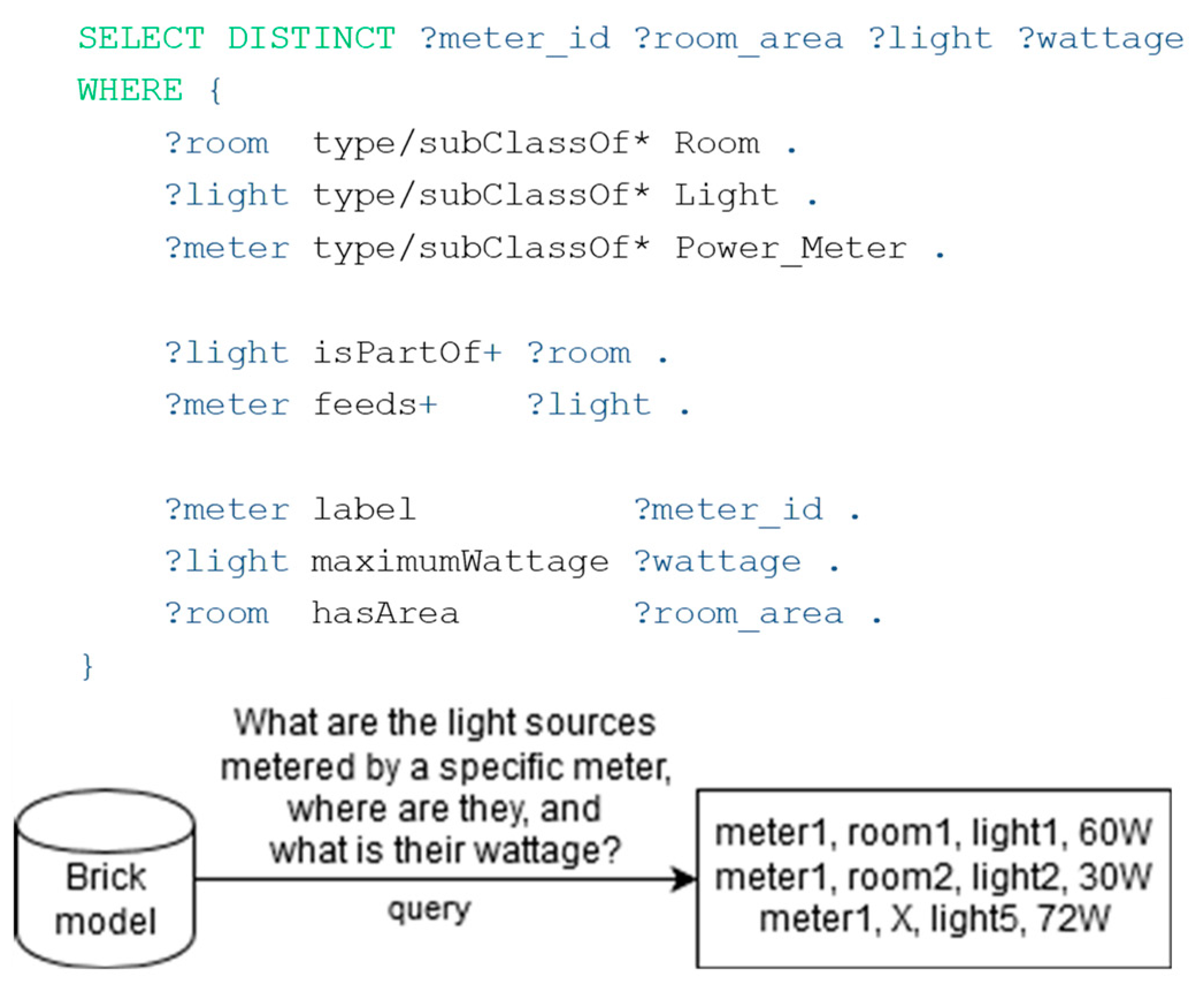
Applications can query a Brick model using the SparQL language. A SparQL query specifies patterns of triples and constraints. In this paper, we show a selection of SparQL queries that have been stripped of namespaces for simplicity. To illustrate, the query in
Figure 3 names three entity variables to extract and lists a set of five restrictions in the WHERE-block. These restrictions define the pattern that the resulting triplets must abide to. Each one defines a path from a subject to an object. This path may be simple or complex in the form of a regular expression-like construct capable of expressing sequence, choice and repetition. Entities with names starting with a question mark are named variables, which can be referenced in the SELECT-block. For every match of the pattern against the underlying RDF store, the query execution engine produces an entry concretizing the named variables from the SELECT-block.
2.3. Procedures for Evaluation of Underperformance
In the following, we present four different procedures for using building metadata models to analyze the output of PTs to discover faults, inconsistencies with the metadata model, or incorrect configuration of the PT. All procedures follow the following algorithm:
A PT is run on various levels of spatial granularity for a period of time;
A list of failed tests and their configurations is generated;
Based on this list, one or more of the proposed procedures are chosen;
The procedure and the list of failed tests are used to produce queries to the metadata model;
The output from the query is postprocessed and analyzed and a potential cause, or set thereof, is identified.
Based on the contents of the list of failed tests and their configurations, different procedures may yield various degrees of benefits. The procedure is chosen based on the coverage of the PT and can be semi-automatically selected based on a list of failed tests and their configurations.
Table 1 presents an overview of the names, requirements, purpose, and potential causes of failed PTs that these procedures may discover. Each of the procedures are explained in detail in the following subsections. Throughout the presentation of the four procedures, we use
Figure 2 to illustrate various examples. The figure does not have a singular meaning and instead is reconfigured for the purpose of the concrete example. Explanations regarding the meanings of the components of the figure will be given for each procedure specifically.
2.3.1. Miswiring Identification Procedure
This procedure has the requirement of the existence of an overall meter on the building level, as well as additional meters for their subsystems that are also wired into the overall meter. If a PT on the overall meter is failing, by examining whether the PT on the submeters wired to it is failing or not, various subsystems can be ruled out as the cause for the failed PT.
Figure 2 illustrates an example of this procedure. On the right side of the figure, meter A has the submeters C, D, and H. We tailor the example to say that the meter H is a submeter of A. We define a PT denoted by P, which evaluates whether the lighting electricity consumption is compliant, while meter H measures the ventilation subsystem electricity consumption. Given this configuration, if the data used for P is from meter A, then the existence of meter H that is a submeter of A implies the need to eliminate H’s contribution to A, since it contains data for another subsystem (ventilation and not lighting). With this, if P is failing and there exists a relationship between A and H, then the potential failing of P might be due to the fact that H is a submeter of A. This implies that a correct result of the PT would be achieved after the elimination of H.
In order to investigate the nature of the meter H, in this procedure we use the query shown in
Figure 3 to extract a mapping from meters to sets of component types and from component types to all more generic types. Such mappings can be used to filter out meters dedicated to measuring components of a specific generic type (e.g., lights). Following the above example, we would like to remove meters measuring components that do not belong to the node types from the lighting system. Metering of any type of ventilation would qualify for exclusion.
2.3.2. Procedure to Discover Presence of Additional Sources
This procedure attempts to detect the existence of unknown components that consume energy under a particular meter. The essence of the procedure lies within the calculation of the theoretical limit for energy consumption for the meter the PT is run for. This theoretical limit represents the amount of consumption in a hypothetical extreme scenario, in which it is assumed that all components metered by a particular meter consume electricity constantly. This is calculated using the metadata model, from which we can extract a detailed array of the hardware that consumes energy and that is ultimately measured by the meter the PT is run on. By taking into account the maximum power for each component type present in the model (e.g., light bulb with highest power) and assuming all of them are being used at the same time, we are able to calculate a value for an exaggerated electricity consumption. This value is known as the theoretical limit. From here, if the timeseries data from a meter exceeds the theoretical limit, then there likely is an additional component being measured by the meter the PT is run on. It is also possible that there is an inconsistency in the metadata model.
Assuming the configuration of the example in
Figure 2, we apply a PT, P, which evaluates whether the consumption from lighting is compliant to the threshold, on the meter X. We define U to be a submeter of meter X, though P is not configured to take this into account, as U’s existence is unknown. If P fails procedure checks whether additional components, which the PT is not configured to take into account, are measured by meter X. This is done through performing a query, which takes into account the power of the electrical components contributing to P—in this case, all components that produce light. Each of these values are summed up and multiplied by the maximum hours in the time period for which P is executed on. The metadata query that is required for this calculation maps meters to the sum of the maximum wattages of all components it meters.
If the consumption of the meter, as calculated in the PT, are higher than the theoretical limit, then we can conclude the existence of an additional component measured by the same meter or an inconsistency with the metadata model. In terms of the example, this means the confirmation of meter U’s contribution to the consumption of meter X. This kind of a result from a PT would potentially be visible from the beginning of the testing; however, it can also appear later on in the lifecycle of the building.
In Brick terms, the procedure needs a mapping from meters to the summed wattage of all lights measured. The query from
Figure 4 collects the wattages of lights being measured by each meter. This is then postprocessed by summing up the wattages per meter to get a theoretical limit of how much the lights can consume.
2.3.3. Procedure to Discover Location of Additional Sources
This procedure aims to discover the location of additional sources that might be measured by an observed meter. This procedure should be applied if suspicion exists that there might be an additional source (for example, after applying the procedure in
Section 2.3.2). Once a query is executed based on the metadata model, it is possible to examine the spatial information of the resulting components. Spatial information may be stored in the form of a string containing a coordinate system tailored to the building, such as office numbers.
In the following, we give a configuration to the example given in
Figure 2, using the tree structure to the right. In this example we assign a PT, P, which evaluates whether the consumption from the lighting subsystem is compliant and uses meter X to acquire the necessary data. From
Figure 2 (to the left) it is obvious that areas A, B, C, D, and E are submetered by the meter X. However, if there is suspicion that an additional component or area exists (meter U), that is being measured by the same meter (X), then a query to the metadata model may be performed. This query would examine the relationships between the meter X used by P and discover all the components that are being measured by it.
By examining the information given regarding the physical location of the components, given as a result from the execution of the metadata query, we may be able to determine which of the components are not present in the same area that P is taking into account. This can be done through examining the location of each component and identifying those that are outside the scope of the PT area or missing location information.
The discovery of additional components that are measured by the same meter that the PT is being run on, which the PT is unaware of, indicates a problem. This problem can resemble an inconsistency between the real world and the metadata model or an underspecified metadata model. Considering the fact that the threshold for the PT is an expected amount of energy per m2, increasing or decreasing the area will yield a different threshold. If the threshold is a different value, whether the test passes or fails might change as well.
The query for this procedure requires a mapping from lights to room names. The query in
Figure 5 extracts this information from the metadata model. Any light without spatial information will be missing from the resulting map.
2.3.4. Procedure to Identify an Underperforming Area
Once a PT fails, it is possible to narrow down the location of a particular underperformance fault. By making use of the metadata model and its information regarding the location of each meter and its respective submeters, we are able to apply a set of rules based on predicate logic and examine the outcomes of various situations.
For
Figure 2 (to the left) if the same PT is applied onto all five meters A, B, C, D, and E, then by producing a truth table from the passing or failing of all five meters, it is possible in some cases to narrow down the area covering the fault. The making of a truth table for all of the meters would imply taking all of the outcomes from the PTs in all of their permutations. This set of situations can then be narrowed down by eliminating some scenarios, such as those where all of the tests are passing or failing. Furthermore, some of the sets will eliminate more areas than others. As this procedure relies on the existence of submeters and reaps the benefits thereof, with increasing the spatial resolution of the meters in an area, i.e., by increasing the number of submeters, the benefits increase. This happens because the existence of more submeters implies the possibility to eliminate more areas, therefore narrowing down the area containing the cause for the underperformance further.
To illustrate this procedure, we present an example using the room drawing in
Figure 2, where all letter symbols denote meters for the area they are assigned to. If the PT for meter A is failing and the PTs for meter C and D are passing, then the fault or underperformance lies within the area of A − (C + D). Similarly, if meter B fails and meter E passes, the area of underperformance is within the area of meter B − E. This kind of rule-based reasoning leads the possibility to calculate the true benefit of the procedure.
The procedure needs a mapping from meters to sets of lamps. We look into two meters MA and MB, which meter the lighting consumption of particular areas. If the set of lamps from meter MA is a proper subset of the set of lamps from meter MB, then MB is closer to the root of the electrical distribution tree, than MA. This allows us to use set operations to reason about the location of the underperforming area. We use the query from
Figure 6 to extract this mapping.
3. Implementation
The following section elaborates on the implementation details of the BuMPeT method. The case building specification has been presented, and appropriate detail has been given with regards to the implementation and setup regarding the PT and the Brick metadata model.
3.1. Case Study Building
The case study building is a new energy efficient teaching building situated in Denmark that became operational at the end of 2015, with about 8500 m2 area containing three levels and one full basement. The building is equipped with a total of 22 m to monitor the electricity consumption from lighting. The basement of the building contains a single meter, while each of the floors contain two meters. Finally, the first floor of the building has three test rooms, each with its own light meters.
For this building, the states of sensors, meters, and actuators are continuously being pulled from the building’s two BMSs (Building Management System) and stored using sMAP [
24] Archiver for easy access. The data from the meters and sensors is stored in a timeseries format. Each timeseries is associated with metadata and queries on this metadata allow us to extract relevant subsets from the available data streams. This paper only relies on data from energy meters, which produce a timeseries stream indicating the accumulated energy usage since installation.
3.2. Implementation of Performance Tests
In this section we provide detailed information of how we obtained the observed and expected behavior of the building. We also provide explanation of the certification tool used to obtain the expected behavior and the calculation used to acquire the observed behavior.
3.2.1. Building Certification Tool
The Danish building energy regulation BR10 was introduced in January 2011, comprising a 25% improvement on the overall energy performance of buildings compared to previous energy classes (14). Two additional future energy classes were added: the low energy class 2015 and the 2020 building energy class, which set strict requirements on the building annual overall energy demand for ventilation, heating, hot water, and lighting. To assess if a building is complying with the BR10 regulations and energy classes, the Danish Building Research Institute (SBi) has developed an energy performance modeling and simulation tool, Be10 [
25], which is the official energy tool for Danish buildings certification based on BR10 regulations. In terms of the modeling and simulation approach, the tool uses a simplified static approach, treating the whole building as one large thermal zone. The tool enables defining static systems parameters in addition to various building constructions with their corresponding area and orientation. However, major assumptions are adopted regarding the loads, schedules, and set points, in addition to neglecting the effect of the weather conditions and the occupancy behavior. Despite this, we consider the outcomes of the model to be valid, as the BE10 modeling tool is a nationally accepted certification tool.
Based on the simulation with the BE10 model, the overall yearly energy consumption of the building is around 41300 Wh/m2. Regarding lighting energy consumption, the tool assumes a standby light intensity of 0.1 W/m2 of the zone area in addition to a nominal light intensity of 3.5 W/m2. Using the assumption of a normal usage for a teaching/office building of operation 9 h per day, 5 days in the week, the BE10 model yields a value of 324 Wh/m2 for lighting in two weeks of normal operation.
3.2.2. Observed Behavior
The PT used within this paper is part of a larger framework that tests various subsystems in the building. Here we focus on the lighting test as it is simple enough to implement, yet complex enough to test the method sufficiently. The test uses the lighting electricity consumption meter data. The electricity consumption is calculated on a 14-day basis. This value is then evaluated to determine whether the PT passes or fails.
The acceptance criterion for this PT is a threshold value +10% with respect to the design numbers derived from the BE10 modeling tool. This ensures that errors within the model that obtained the threshold will be deliberately overcompensated. If the result of the PT is higher than the threshold, the PT fails, otherwise it passes.
The Section regarding the real scenario under Experiments and Evaluation, gives information about the available metering. As each floor aside from the basement contains 2 m, the PT has been run both for each half floor, respectively, but also on a whole floor level. The PT was executed on the entirety of the available data, yielding results for the lighting performance of the whole building for nearly a year of its usage. Our results are saved as separate data streams within the same sMAP Archiver.
3.3. Implementation of Brick Model
Given our focus on the lighting system, the parts of the case study building that are relevant to our PT include the electrical distribution tree with positions of meters and lamps, and which rooms these lamps located in. More specifically, we need to be able to map a meter to a covered area (the union of all rooms containing lamps measured by the meter) and a maximum wattage (the sum of the maximum wattages of all lamps measured by the meter).
To support this mapping, we modeled the case study building in a version of Brick what we extended in three ways: (i) the meters were associated with an ID for reference—the same one that they have in the archiver; (ii) the lights we associated with a maximum power; and (iii) the rooms were associated with a surface area. Each of these annotations are encoded as RDF literals. For portability, both the power and the area mention their SI unit explicitly.
Figure 7 highlights the basic structure on which queries are resolved. The full graph references 22 m, 929 lights, and 222 rooms.
The data for populating the model was manually extracted and linked from three sets of technical drawings covering the electrical distribution tree, the lighting system (type and wattage), and base room information (area).
In an effort to verify that the model is both consistent and a good representative of the case study building we have performed a selection of sanity checks. To do this we added room type to the model and verified that area and light power density followed a Gaussian distribution for each room type. We also added room names that contain the floor in the string of their name and used this to verify the room → floor map.
4. Experiments and Evaluation
The results from the PT and the Brick model provide solid ground for evaluating BuMPeT. A real case scenario of failing performance tests has been resolved through the usage of the method, with the aid of the Procedure to discover presence of additional sources and the Procedure to discover location of additional sources. A hypothetical scenario has been created to evaluate the Procedure to identify an underperforming area and the Miswiring Identification Procedure. In this section, also, we take
Figure 2 to be a generic example that we tailor to the specific needs of the concrete examples.
4.1. Real Scenario
4.1.1. Basement Underperformance
Figure 8 shows results of PTing of the lighting in the basement from February 2016 until the beginning of January 2017. The initial threshold was obtained using the BE10 model, as a function of the light electricity consumption per m
2, multiplied by the total area of the basement which is 1818 m
2. Thus, we get the initial threshold of 587,000 Wh/14 days. To factor in errors, we deliberately overestimate by adding 10% to the original threshold, achieving a value of 645,000 Wh/14 days. The results show a significant amount of data points that are higher than the threshold.
As these failed performance tests might indicate a potential underperforming component or errors of different nature, two of the procedures in the Implementation Section were applied. The theoretical limit (
Section 2) was calculated to discover whether the results from the test were higher than this limit. This calculation was done by querying each light component in the basement from the Brick model using the query from
Figure 9 and summing up their wattages which is 3355W. We then calculated that the theoretical threshold is 1,127,000 Wh/14 days, assuming every lamp being on for the entire period. Considering that there are still many data points that are above the theoretical limit, we concluded that there were additional components being measured by the meter that the PT was not taking into account. This implies either an incorrectly configured PT as its configuration does not reflect reality or a physical miswiring error.
To further investigate these additional components, the query from
Figure 10 was executed to the Brick model to examine the components that were being measured by the basement light meter, according to the Procedure to discover location of additional sources in
Section 2.3.2. The query resulted in 117 components, 8 of which were found to be emergency lighting (which were not on during the timeframe under analysis). Further processing revealed that two of the 108 remaining components were not associated with a specific room.
Reviewing the technical documents revealed the existence of a green wall and outdoor lighting components that were measured by the same meter. With this discovery, the reason for the underperformance of the basement was found to be a miswiring issue. After alerting the building managers, the outdoor lighting and the green wall were wired to a separate meter. The PT and the metadata model were changed accordingly.
An alternative path for investigation could have been to apply the Procedure to identify an underperforming area. However, considering that the basement did not have any submeters for the lighting, the requirements for this procedure were unfulfilled.
4.1.2. Parterre Underperformance
The parterre in the case building is a floor with two meters. The results of the PTing for a year for the meters on this floor are shown in
Figure 8. Failure of the PT is evident around June and December 2016.
The thresholds for the PT are obtained as a function of their areas and the expected consumption based on the BE10 model. As the areas are 1360 and 945 m2 for the south and half floor, respectively, the thresholds are 440,000 Wh/14 days and 306,000 Wh/14 days, respectively, while the overall floor’s threshold is 746,000 Wh/14 days.
Considering there is a submeter for lighting in the Parterre, we apply the Procedure to identify an underperforming area to narrow down the area of underperformance. Thus, we perform the test separately for the two half floors. For the failed test in June, it is evident that the PT for lighting consumption for the north half fails, while the south one doesn’t, eliminating the area of the fault to the north half floor only. For the failed test in December, both PTs for the half floors fail for the same time interval, which means that no gain has been achieved from this procedure. In both cases we suspect that the violation is due to changes in occupancy patterns of the building close to the exam period.
4.1.3. Analysis of Procedure to Discover Presence of Additional Sources
To evaluate this procedure, we look into the case of the underperformance in the basement. We examine the extent to which the theoretical limit could be overestimated and still produce insights in our particular case. For the procedure to be applicable, there needs to be a value in the observed behaviour in the PT which is still higher than the overestimated theoretical limit.
Table 2 presents the configuration of lights for the examined area, showing wattage and count, for each class of lights. The overestimated theoretical limit is achieved by discovering the number of lights that are possible to be changed (with increased wattage), while the total maximum still yields a value lower than the highest point in the observed behavior from the PT. Two of the lights are already rated at 60W, meaning that it is a matter of discovering how many additional lights would be able to be changed (by mistake, or in the model). We do this by assigning a certain percentage of lights to be changed to 60W, while the distribution of the remaining lights is unchanged. In order to search through various possibilities, we have run a script that explored various configurations of percentages of lights changed. The results from the execution of the script show that if 53 of the total lights are 60W and the rest of them maintain the same percentage of contribution to the consumption that they have had in the initial configuration, the theoretical limit would be the highest possible while still lower than the highest of the results from the PT.
In
Table 2, the column “Contribution to old configuration (%)” reveals the percentage with which each of the classes of lights is contributing to the setup of lights per class. The two lights already having 60W are not taken into account, as they are already at their maximum, and we are searching for a configuration for the rest of the lights. Thus, the percentages are calculated out of 105 lights, since we have removed the two out of the original 107. The column “Contribution to new configuration scaled to remaining lights (54)” is calculated by multiplying the percentage out of 105 lights and the number of remaining lights, 54. This way, the new configuration of lights are 53 60W lights, and each row of the fourth column multiplied by its respective wattage. By multiplying this wattage by 336 working hours (representing a two week period), we achieve 1,627,488 Wh/14 days.
These values imply that if 49% of the lights assume the maximum wattage of all lights, the procedure would still be applicable. Considering that some of the lights are already with maximum wattage, if 47% of the lights in the basement were replaced by the maximum wattage lights, the procedure would still be able to detect an additional component that is measured by the same meter.
4.1.4. Analysis of Location of Additional Sources Procedure
In the case of the scenario of basement underperformance, this procedure was applied by querying the Brick model for all of its components that are measured by the basement light meter, yielding the successful discovery of the green wall and outdoor lighting.
4.2. Hypothetical Scenario
4.2.1. First Floor Underperformance
To create a hypothetical scenario, we use the floor plan shown on the left side in
Figure 2. This figure illustrates the first floor of the case study building, where the lights in the areas A and B are measured by separate meters. The areas C, D, and E are test rooms that have been equipped with light meters. We apply the Miswiring Identification Procedure and the Procedure to identify an underperforming area and discuss their benefits within a hypothetical scenario. For the application of the Miswiring identification Procedure, meter H is considered to be a submeter of meter A. For the application of the Location of underperforming area procedure, meter H is not a submeter of meter A.
First Floor Miswiring Identification Procedure
As shown in Figure, meter H is metering the electricity consumption of an HVAC component, and is a submeter to meter A. We define a lighting PT, P, that is run on meter A. In the event that P fails, one procedure to be applied would be the Miswiring identification Procedure to discover whether meter A has any submeters that do not belong to the lighting subsystems. A query to the Brick model would yield a result that shows all submeters of A: C,D,H. Further postprocessing discovers that H is a meter for the ventilation subsystem. Therefore, if P was executed on A, it could need to be configured correctly, so that P does not consider the consumption metered by H.
4.2.2. Analysis of Miswiring Identification Procedure
In the case of the hypothetical scenario in the example of the meter H being a submeter of meter A, this procedure was applied to discover if any of A’s submeters belonged to another subsystem. By querying the Brick model for all of A’s submeters, it was discovered that the meter H contained information indicating its belonging to the ventilation system. Thus, the source of the underperformance was detected.
4.2.3. Analysis of Location of Underperforming Area Procedure
The evaluation has been performed for the first floor of the case building.
Table 3 provides an overview of the percentage of area available to be eliminated. In the situations where the result of a meter or submeter is irrelevant, such as a situation evaluating only one-half floor, NA has been used in the table.
According to
Table 3, the lowest benefit is in the scenario of the north half floor. The highest benefit is obtained in the event that the meter for overall floor PT fails, while one of the half floors fail. Given the large amount of area that was eliminated due to the presence of three submeters, in this case, we conclude that the benefits are proportional to the number of submeters.
5. Related Work
Previous work has already explored PTing for FDD (8) by applying expert knowledge rules for assessment of measured data. For more detailed pinpointing of faults, Mcintosh applied a model-based FDD method comparing simulation results to measured data. In an effort that relates the concepts of FDD and PTing, Stylianou et al. [
26] focused on reciprocating chillers, assuming very detailed knowledge of the particular chiller for their method. Various FDD approaches that utilize historical data are also related to PTing but often the tested thresholds are not based on building certificates. One example is the approach for real-time detection of anomalies presented by Chou et al. [
27], which is based on comparison of real and predicted consumption by applying the two-sigma rule. These approaches use highly detailed models for predicting the expected behavior of a particular component, while BuMPeT is flexible in this sense, and able to work with various kinds of models, regardless of the complexity of their design and usage.
FDD approaches that integrate Building Information Models (BIMs) are also relevant to our method. Existing BIMs, however, only cover a subset of the relevant relationships that Brick is able to represent [
16]. Shi et al. [
28] present a method for using building information models for semi-automatic constructing models for model-based FDD. However, a large proportion of the model parameters are still set by manual surveys or calibrated from historical data. Costa et al. [
6] present a method that from a building information model generates relevant PT cases. However, for detailed fault diagnosis they apply a model-based approach without a direct coupling to the PTs. Another building information model enabled approach has been described by Dong et al. [
7]. This approach integrates a simulation module, a module for static and dynamic information as well as a separate FDD module. While it presents good experimental results, the effort to prepare the information infrastructure necessary for the FDD process is greater than the effort the implementation of BuMPeT would take. Moreover, the modules are not connected.
In comparison, BuMPeT builds on the more descriptive building metadata models. It provides a direct link between PTs and the procedures for narrowing down faults within a building. Furthermore, the results in this paper document the benefits of the method when applied to a real case building. Application to a new building is only conditioned by the availability of the building’s metadata model.
The case study in [
29] has been applied to the HVAC system only, without further information on how to extend the methodology onto other subsystems. One limitation of the proposed system is that it depends on human input, i.e., occupants are expected to submit tickets upon experiencing deteriorated performance of the HVAC. This is a shortcoming as faults or underperformance may emerge long before the occupants experience them and report them. The development of this approach seems to be relatable to a single BIM within the case study and lacks applicability to other BIMs without an extensive integration period. Contrary to this, our approach BuMPeT is based on PTing that utilizes building instrumentation, and thus requires no user input. Furthermore, it is easily extendable to other buildings and their respective BIMs. The ability for the PT framework to automatically discover and instantiate the applicable PTs from a metadata model supports its flexibility and portability [
30].
Sunnam et al. in [
31] analyze a case study that incorporates observation of actual building measurement data and comparisons of the observations with the design’s intent. However, this comparison is done by consulting a commissioning engineer, which presents a drawback in the approach as it is time consuming and likely expensive. The classified data is then analyzed within another module that is not fluently integrated and automatic, presenting another disadvantage. Conversely, BuMPeT’s executions of tests are automatic, both the discovery of thresholds for the tests, as well as the execution of the procedures proposed in this paper.
The approach in [
13] uses a semantic model very similar to the Brick model, whose extensibility to additional subsystems requires introduction of additional semantic models, while Brick already incorporates them. This significantly limits the applicability of the presented approach to other subsystems, which is not the case with BuMPeT. The same research group in [
32] has also developed an approach using Brick that performs FDD through the extraction of knowledge regarding component relationships from a physical model of the building. The authors in [
33] create a framework using the Jena API by Apache, used to extract data from and write to RDF graphs. The creation of the metadata in digital formats, however, requires prior human effort, similar to the creation of a Brick model.
6. Discussion and Future Work
Common practice does not yet incorporate large metadata models that include all of the data related to a building. Therefore, it is of high importance to examine the effort required to produce a metadata model. The initialization and set up of the Brick model used within this effort took approximately 20 h. The addition of the information related to the lighting system took 30 h, resulting in a workload of only 50 h for a model of the lighting subsystem. This data was acquired from technical documents, mainly stored in PDF format. Expanding the model with all subsystems is expected to take no longer than 150 h, including performing some basic plausibility checks. Despite the requirement of 150 h to produce the full metadata model, we believe that it is an improvement in comparison to the manual instantiation of PTs and the manual search for faults in a building. We expect that the general trend of buildings will expand to a situation where metadata models are handed over with new buildings. In this case, the production of the metadata model would fall into the hands of a qualified person within the contractor company and the metadata model would be under development in parallel with the building, reducing these initial effort hours to a minimum. In the case of the Brick schema, however, it is possible to derive a partially complete Brick model based on IFC building information models, which are far more commonly available [
17]. The maintenance of the model is a matter of continuous attention.
Furthermore, the current procedures are semi-automated and still require human help to reason out the true causes of failed PTs. We expect that these procedures would be a part of a more complex system which would intelligently discover when to apply which, and also how best to utilize their results.
Future work heavily relies on expanding the test suite with additional PTs. The growth of the set of implemented PTs also implies the expansion of the metadata model. Creating procedures that use the results from PTs which are not only lighting-related will expand the FDD reasoning to the interactions with the rest of the subsystems.
7. Conclusions
This paper proposes the usage of PTing in the aid of FDD. We presented the BuMPeT method, which uses a metadata model to extend PTing with FDD capabilities. The BuMPeT method presents four procedures, able to narrow down the pool of possible faults causing a filed PT, using metadata queries. The proposed method has been applied to a case study building to assess its validity and benefits, focusing predominantly on experiments with the lighting system in the building. As a threshold for PTs, the BE10 building modeling tool has been used, which reflects Danish building regulations.
Within this paper, we have examined the extent to which the four procedures comprising the BuMPeT method can aid the FDD process, through examining two real scenarios from a case study building, and two hypothetical scenarios. As a result, the Procedure to discover presence of additional sources and the Procedure to discover location of additional sources have been successfully applied to discover the reason for a failed PT. In one case, the failure of a PT was tied to incorrect meter wiring from outdoor lighting and into the meter from the basement. In the second case, the failure of the PT was linked to fluctuations in occupancy schedules due to exam seasons. This paper further examined a hypothetical scenario in which different subsets of the meters failed a PT. In this case, we evaluated the Miswiring Identification Procedure and Procedure to identify an underperforming area. In the best case, the area of the fault was narrowed down by 46% of the total floor area. The results of the application of this method demonstrate that the symbiosis of metadata and performance testing produce insights into the detection and diagnosis of errors or faults in a highly complex workflow that includes people, software, hardware, and data.
Usage of metadata models to describe buildings’ metadata is a part of the movement for the future development of the building industry. Providing machine-readable technical documentation during building-handover is key to automating various FDD and PTing processes. The development of the BuMPeT method in light of PTing and FDD is a clear step towards automating FDD without human input.
Author Contributions
E.M. and A.J. fully conceptualized the BuMPeT method. E.M. wrote the majority of the manuscript, developed the performance tests, calculated the performance test results, and visualized their results. A.J. developed the Brick model and a tight collaboration formed the Brick queries within the procedures. M.B.K. contributed through general supervision of the development of the BuMPeT method, reviewing the manuscript, and editing it. S.L.-M. reviewed and edited the manuscript, in addition to reflecting on the FDD aspects of performance testing in light of BuMPeT. M.J. supervised the developed method and reviewed the manuscript, in particular the sections about the BE10 model. B.N.J. contributed through funding acquisition, supervision of the first author, and reviewing the manuscript.
Funding
This research was carried out under COORDICY Project, funded by Innovation Fund Denmark, ID number: 4106-00003B.
Conflicts of Interest
The authors declare no conflict of interest. The funders had no role in the design of the study; in the collection, analyses, or interpretation of data; in the writing of the manuscript, or in the decision to publish the results.
References
- Cao, X.; Dai, X.; Liu, J. Building energy-consumption status worldwide and the state-of-the-art technologies for zero-energy buildings during the past decade. Energy Build. 2016, 128, 198–213. [Google Scholar] [CrossRef]
- Scofield, J.H. Efficacy of LEED-certification in reducing energy consumption and greenhouse gas emission for large New York City office buildings. Energy Build. 2013, 67, 517–524. [Google Scholar] [CrossRef]
- Markoska, E.; Jradi, M.; Jorgensen, B.N. Continuous commissioning of buildings: A case study of a campus building in Denmark. In Proceedings of the 2016 IEEE International Conference on Internet of Things (iThings) and IEEE Green Computing and Communications (GreenCom) and IEEE Cyber, Physical and Social Computing (CPSCom) and IEEE Smart Data (SmartData), Chengdu, China, 15–18 December 2016. [Google Scholar]
- Markoska, E.; Lazarova-Molnar, S. Towards smart buildings performance testing as a service. In Proceedings of the 2018 Third International Conference on Fog and Mobile Edge Computing (FMEC), Barcelona, Spain, 23–26 April 2018. [Google Scholar]
- Markoska, E.; Lazarova-Molnar, S. LEAF: Live building performance evaluation framework. In Proceedings of the Fourth International Conference on Fog and Mobile Edge Computing (FMEC), Rome, Italy, 10–13 June 2019. [Google Scholar]
- Costa, A.; Keane, M.M.; Torrens, J.I.; Corry, E. Building operation and energy performance: Monitoring, analysis and optimisation toolkit. Appl. Energy 2013, 101, 310–316. [Google Scholar] [CrossRef]
- Dong, B.; O’Neill, Z.; Li, Z. A BIM-enabled information infrastructure for building energy fault detection and diagnostics. Autom. Constr. 2014, 44, 197–211. [Google Scholar] [CrossRef]
- Mattera, C.G.; Jradi, M.; Shaker, H.R. Online energy simulator for building fault detection and diagnostics using dynamic energy performance model. Int. J. Low Carbon Technol. 2018, 13, 231–239. [Google Scholar] [CrossRef]
- McIntosh, I.B.D. A Model-Based Fault Detection and Diagnosis Methodology for HVAC Subsystems. Ph.D. Thesis, University of Wisconsin-Madison, College of Engineering, Madison, WI, USA, 1999. [Google Scholar]
- Bazjanac, V.; Crawley, D. Industry foundation classes and interoperable commercial software in support of design of energy-efficient buildings. In Proceedings of the Building Simulation’99, Kyoto, Japan, 13–15 September 1999. [Google Scholar]
- Compton, M.; Barnaghi, P.; Bermudez, L.; García-Castro, R.; Corcho, O.; Cox, S.; Graybeal, J.; Hauswirth, M.; Henson, C.; Herzog, A.; et al. The SSN ontology of the W3C semantic sensor network incubator group. J. Web Semant. 2012, 17, 25–32. [Google Scholar] [CrossRef]
- Karger, D.R.; Bakshi, K.; Huynh, D.; Quan, D.; Sinha, V. Haystack: A customizable general-purpose information management tool for end users of semistructured data. In Proceedings of the 2nd Biennial Conference on Innovative Data Systems Research (CIDR), Asilomar, CA, USA, 4–7 January 2005. [Google Scholar]
- Ploennigs, J.; Clement, J.; Wollschlaeger, B.; Kabitzsch, K. Semantic models for physical processes in CPS at the example of occupant thermal comfort. In Proceedings of the 2016 IEEE 25th International Symposium on Industrial Electronics (ISIE), Santa Clara, CA, USA, 8–10 June 2016. [Google Scholar]
- Huynh, D.; Karger, D.R.; Quan, D. Haystack: A Platform for creating, organizing and visualizing information using RDF. In Proceedings of the Semantic Web Workshop, Florence, Italy, 13–17 October 2002. [Google Scholar]
- Daniele, L.; Hartog, F.D.; Roes, J. Created in Close Interaction with the Industry: The Smart Appliances REFerence (SAREF) Ontology; Springer Science and Business Media LLC: Larkspur, CA, USA, 2015; Volume 225, pp. 100–112. [Google Scholar]
- Balaji, B.; Bhattacharya, A.; Fierro, G.; Gao, J.; Gluck, J.; Hong, D.; Johansen, A.; Koh, J.; Ploennigs, J.; Agarwal, Y. Brick: Towards a unified metadata schema for buildings. In Proceedings of the 3rd ACM International Conference on Systems for Energy-Efficient Built Environments, Palo Alto, CA, USA, 16–17 November 2016. [Google Scholar]
- Balaji, B.; Bhattacharya, A.; Fierro, G.; Gao, J.; Gluck, J.; Hong, D.; Johansen, A.; Koh, J.; Ploennigs, J.; Agarwal, Y.; et al. Brick: Metadata schema for portable smart building applications. Appl. Energy 2018, 226, 1273–1292. [Google Scholar] [CrossRef]
- Jørgensen, B.N.; Kjærgaard, M.B.; Lazarova-Molnar, S.; Shaker, H.R.; Veje, C.T. Challenge: Advancing energy informatics to enable assessable improvements of energy performance in buildings. In Proceedings of the 2015 ACM Sixth International Conference on Future Energy Systems, Bangalore, India, 14–17 July 2015. [Google Scholar]
- Lange, C.; Kosiankowski, D.; Weidmann, R.; Gladisch, A. Energy consumption of telecommunication networks and related improvement options. IEEE J. Sel. Top. Quant. Electron. 2010, 17, 285–295. [Google Scholar] [CrossRef]
- Han, D.-M.; Lim, J.-H. Smart home energy management system using IEEE 802.15.4 and zigbee. IEEE Trans. Consum. Electron. 2010, 56, 1403–1410. [Google Scholar] [CrossRef]
- Marsan, M.A.; Chiaraviglio, L.; Ciullo, D.; Meo, M. Optimal energy savings in cellular access networks. In Proceedings of the 2009 IEEE International Conference on Communications Workshops, Dresden, Germany, 14–18 June 2009. [Google Scholar]
- EMD. The Danish Ministry of Economic and Business Affairs—BR10 Danish Building Regulation; EMD: Copenhagen, Denmark, 2010. [Google Scholar]
- Crawley, D.B.; Lawrie, L.K.; Winkelmann, F.C.; Buhl, W.; Huang, Y.; Pedersen, C.O.; Strand, R.K.; Liesen, R.J.; Fisher, D.E.; Witte, M.J.; et al. EnergyPlus: Creating a new-generation building energy simulation program. Energy Build. 2001, 33, 319–331. [Google Scholar] [CrossRef]
- Dawson-Haggerty, S.; Jiang, X.; Tolle, G.; Ortiz, J.; Culler, D. sMAP: A simple measurement and actuation profile for physical information. In Proceedings of the 8th ACM Conference on Embedded Networked Sensor Systems, Zürich, Switzerland, 3–5 November 2010. [Google Scholar]
- SBI. The Danish Building Research Institute—BE10 SBI Tool; SBI: Copenhagen, Denmark, 2010. [Google Scholar]
- Stylianou, M.; Nikanpour, D. Performance Monitoring, Fault Detection, and Diagnosis of Reciprocating Chillers; American Society of Heating, Refrigerating and Air-Conditioning Engineers, Inc.: Atlanta, GA, USA, 1996. [Google Scholar]
- Chou, J.-S.; Telaga, A.S. Real-time detection of anomalous power consumption. Renew. Sustain. Energy Rev. 2014, 33, 400–411. [Google Scholar] [CrossRef]
- Shi, Z.; Abdelalim, A.; O’Brien, W.; Attar, R.; Akiki, P.; Graham, K.; Van Waarden, B.; Fai, S.; Tessier, A.; Khan, A. Digital campus innovation project: Integration of building information modelling with building performance simulation and building diagnostics. In Proceedings of the Symposium on Simulation for Architecture & Urban Design, Washington, DC, USA, 12–15 April 2015. [Google Scholar]
- Golabchi, A.; Akula, M.; Kamat, V. Automated building information modeling for fault detection and diagnostics in commercial HVAC systems. Facilities 2016, 34, 233–246. [Google Scholar] [CrossRef]
- Markoska, E.; Johansen, A.; Lazarova-Molnar, S. A Framework for Fully Automated Performance Testing for Smart Buildings. In Proceedings of the Third International Congress on Information and Communication Technology, London, UK, 27–28 February 2018. [Google Scholar]
- Sunnam, R.; Ergan, S.; Akinci, B. Deviation analysis of the design intent and implemented controls of HVAC systems using sensor data: A case study. Comput. Civ. Eng. 2015, 2015, 223–231. [Google Scholar]
- Ploennigs, J.; Maghella, M.; Schumann, A.; Chen, B. Semantic Diagnosis Approach for Buildings. IEEE Trans. Ind. Inform. 2017, 13, 3399–3410. [Google Scholar] [CrossRef]
- Delgoshaei, P.; Austin, M.A. Framework for knowledge-based fault detection and diagnostics in multi-domain systems: Application to heating ventilation and air conditioning systems. Int. J. Adv. Syst. Meas. 2017, 10, 393–409. [Google Scholar]
Figure 1.
Overview of the Building Metadata Performance Testing (BuMPeT) method. FDD: fault detection and diagnostics.
Figure 1.
Overview of the Building Metadata Performance Testing (BuMPeT) method. FDD: fault detection and diagnostics.
Figure 2.
Example floor of the case building with lights and the feeds relationships of the electrical distribution tree. A, B, C, D, E and H are submeters, X is a main meter, and U is an unknown component being fed by meter X.
Figure 2.
Example floor of the case building with lights and the feeds relationships of the electrical distribution tree. A, B, C, D, E and H are submeters, X is a main meter, and U is an unknown component being fed by meter X.
Figure 3.
On the left, a SPARQL query for collecting enough information to construct a mapping from meter to sets of component types (and their chain of superclasses) fed by that meter. An illustration of the query question and example results on the right.
Figure 3.
On the left, a SPARQL query for collecting enough information to construct a mapping from meter to sets of component types (and their chain of superclasses) fed by that meter. An illustration of the query question and example results on the right.
Figure 4.
Query for collecting the wattages of lights being fed by each meter in SPARQL on the left. The sets are constructed from individual pairs in post processing. An illustration of the query question and example results on the right.
Figure 4.
Query for collecting the wattages of lights being fed by each meter in SPARQL on the left. The sets are constructed from individual pairs in post processing. An illustration of the query question and example results on the right.
Figure 5.
Query for collecting spatial information about lights in SPARQL on the left and an illustration of the query question and example results on the right.
Figure 5.
Query for collecting spatial information about lights in SPARQL on the left and an illustration of the query question and example results on the right.
Figure 6.
Query for collecting the sets of lights being fed by each meter in SPARQL on the left. The sets are constructed from individual pairs in post processing. An illustration of the query question and example results on the right.
Figure 6.
Query for collecting the sets of lights being fed by each meter in SPARQL on the left. The sets are constructed from individual pairs in post processing. An illustration of the query question and example results on the right.
Figure 7.
Substructure of Brick model relevant querying, showing how meters (M), lights (L), and rooms (R) are linked.
Figure 7.
Substructure of Brick model relevant querying, showing how meters (M), lights (L), and rooms (R) are linked.
Figure 8.
Plots of performance test results.
Figure 8.
Plots of performance test results.
Figure 9.
Query for collecting per light maximum wattages. The wattages are summed up per meter in post processing.
Figure 9.
Query for collecting per light maximum wattages. The wattages are summed up per meter in post processing.
Figure 10.
Query for collecting per meter light list.
Figure 10.
Query for collecting per meter light list.
Table 1.
Procedures for evaluation of underperformance.
Table 1.
Procedures for evaluation of underperformance.
| Name | Purpose | Requirements | Potentially Discovered Causes for Underperformance |
|---|
| Miswiring identification procedure | Investigation regarding which subsystem is responsible for a holistic underperformance | Existence of meters for various subsystems in the building, as well as overall meter | Identification of underperforming subsystem.
Incorrectly configured performance tests (PT)
Incorrect metadata in model |
| Procedure to discover presence of additional sources | Discovery of the existence of additional components feeding into a meter | Highly detailed metadata for calculating a theoretical limit | Identification of incorrectly wired components metered by a meter.
Incorrectly configured PT
Incorrect metadata in model |
| Procedure to discover location of additional sources | Discovery of the physical location of components that are feeding into a meter | Existence of location specifics for each component in the metadata | Discovery of physical location of incorrectly wired components metered by a meter.
Incorrectly configured PT
Incorrect metadata in model |
| Procedure to identify an underperforming area | Narrowing down the physical area in which the underperformance is occurring | Existence of submetering with higher spatial granularity | Identifying an area (or subset thereof) of underperformance.
Incorrectly configured PT
Incorrect metadata in model |
Table 2.
Discovery of applicability limit.
Table 2.
Discovery of applicability limit.
| Wattage (Class) | No. of Lights | Contribution to Old Configuration (%) | Contribution to New Configuration Scaled to Remaining Lights (54) |
|---|
| 10 | 10 | 9.34 | 5.13 |
| 14 | 6 | 5.6 | 3.078 |
| 15 | 8 | 7.47 | 4.104 |
| 31 | 7 | 6.54 | 3.564 |
| 36 | 69 | 64.48 | 35.478 |
| 46 | 5 | 4.67 | 2.538 |
| 60 | 2 | removed | removed |
Table 3.
Evaluation of Location of underperforming area strategy.
Table 3.
Evaluation of Location of underperforming area strategy.
| X | A | B | C | D | E | Elim. Area |
|---|
| NA | F | NA | P | P | NA | 19% |
| NA | F | NA | P | F | NA | 9% |
| NA | F | NA | F | P | NA | 9% |
| NA | NA | F | NA | NA | P | 20% |
| F | P | F | P | P | P | 74% |
| F | F | P | P | P | P | 45% |
© 2019 by the authors. Licensee MDPI, Basel, Switzerland. This article is an open access article distributed under the terms and conditions of the Creative Commons Attribution (CC BY) license (http://creativecommons.org/licenses/by/4.0/).


 ,
, 


