1. Introduction
Nowadays, the attention paid by various societal components to the negative impacts of a global energy supply based largely on fossil fuels is significant [
1]. This is reflected by the many public funding schemes or policies set up at the local, national or international level with the clear intent to orient the scientific and technological development towards energy efficiency and carbon-free energy sources [
2]. The EU Horizon 2020 framework program and the national incentives schemes to advance renewable energy sources are citable examples. International Energy Agency data support the idea that despite the intense development and competition among rival renewable energy sources, a high unexploited potential for the development and diffusion of solar thermal systems still persists [
3,
4]. Experts in the field also believe that the market for solar thermal systems will profit from a cost-reducing innovation step, considering its current period of stagnation.
The natural purpose of the solar system designer is to maximize the solar energy collected and delivered to the load. To achieve this goal, the traditional (local, without a supervisor) control of discrete components utilising proportional, proportional and integral, or proportional–integral–derivative (P, PI or PID) controllers is not always adequate, as it would be the management of all of the solar system components at the global level, enabling optimal control strategies to be implemented. The implementation of complex feedback control strategies requires a certain number of computations. For this reason, a digital controller is usually a component of modern solar systems. The definition of simple algorithms with a small memory footprint is of particular interest, as such algorithms can be implemented on very low-cost hardware.
In such a framework, cost-saving opportunities arise because the optimal control strategy to achieve the best performance is usually devised heavily relying on time-consuming and computationally intensive numerical simulations. Such simulations are performed at various stages of the design process: (a) to validate the models of the single components of the system; (b) to validate the integrated system as a whole; and (c) to develop the control strategy. Stage (a) is often an iterative process which may involve collecting experimental data from prototypes. Stage (b) may also involve a comparison with field data if the solar system (or plant) to be optimized already exists. In stage (c), the model of the plant is extensively used to perform parametric analyses of the plant model and/or optimizations of the closed loop system.
Another opportunity for cost-savings, in the form of reduced backup systems use due to higher solar energy gains, arise in the case of small solar systems because they often get installed directly by personnel lacking control experience, and an on-field optimization of the control strategy is simply not performed, resulting in the underperformance of the installed systems.
The idea behind this work is to reduce the time spent on modelling and simulations during the design of optimized controllers for solar thermal systems. To attain this goal, a self-learning controller has been designed applying the methods of reinforced learning (RL) and fuzzy control (FC). After a learning phase, the controller can optimize its internal control parameters without the need of finding them a priori through simulations. In this work, controller performance was evaluated using a mathematical model of a simple, well-known solar thermal system. The performance of this coupled RL/FC controller has been compared to other control practices, such as traditional on/off, proportional feedback control and FC. The original work presented in Reference [
5] is here extended by providing an extended literature review, a detailed description of the algorithm used, and additional results about the effect of membership functions and the impact of RL parameters.
The paper is organized into sections and subsections. The rest of the introductory section sets the background regarding the FC topic (
Section 1.1) and RL topic (
Section 1.2) and reviews the applications of traditional control (
Section 1.3), fuzzy control (
Section 1.4), and reinforcement learning (
Section 1.5) to solar thermal systems or to energy management systems. Moreover, a review of the joint application of FC and RL is therein given (
Section 1.6).
Section 2 describes the method and techniques used to implement the controller and the tool used to assess its quality. In particular, this section covers how a guided exploration was added to the original Q-learning algorithm (
Section 2.1), how the algorithm was modified to allow full and partial reset of acquired knowledge (
Section 2.2), how the coupling between FC and RL was implemented (
Section 2.3), the layout of the domestic hot water system used to run simulations (
Section 2.4), and the performance figures used to assess the controller(s) (
Section 2.5).
Section 3 discusses the simulation results which are organized into: results of the reference cases (
Section 3.1), results of the FC alone (
Section 3.2), results of the RL controller alone (
Section 3.3), and results of the joint FC–RL controller. Concluding remarks and options for future developments are given in
Section 4.
1.1. Fuzzy Logic Controllers
Fuzzy logic (FL) is a method of rule-based decision making used for expert system and process control. Fuzzy logic is based on the fuzzy-sets theory, which relates to classes of objects with vaguely defined boundaries in which membership is a matter of degree. This logic was developed by Lofti Zadeh in the early 1960s as a way to model the uncertainty of natural language [
6,
7,
8], and since then it has been successfully applied to several areas of science and technology, and in particular to system control [
9,
10].
A fuzzy controller (FC) is commonly defined as a control system that emulates a human expert using the principles of FL. The key elements of an FC are a set of “if–then” rules (knowledge-base), an internal logic processor (inference mechanism), and two components called fuzzifier and de-fuzzifier [
11]. The rules, in the form “IF
is
THEN
is
”, determine the conclusions of the inference mechanism in a similar way premises determine the conclusions of a deduction engine based on classical logic (the inference process follows the so-called modus ponendo ponens: given the rule “IF
is
THEN
is
. ” and the fact that
is
percent
it concludes that
is
percent
). In the implementation of the FC used in this work, the Mamdani fuzzy inference system was considered. This inference system is characterized by a linguistic variable in the “then” clause of the rules base. The fuzzifier and de-fuzzifier solve the problem of mapping the scalar variables to fuzzy objects that can be processed by the inference engine and vice-versa. In a Mamdani system, membership functions (functions from the domain of real numbers to the closed interval [0,1],
) need to be defined for the input and output variables. Attention should be paid to the definition of the membership functions, overlapping them in order to obtain a regular control curve [
12]. Three overlapping triangularly shaped membership functions for both the input and output quantity. Triangularly shaped functions have been chosen because they are easy to evaluate and are described by only three parameters. Regarding the de-fuzzifier, several methods exist to compute a numeric value from a set of partially true conclusions. The centre of gravity de-fuzzification method was selected because, according to what has been found in the literature, it is currently the most used in concrete applications [
13]. The combination of fuzzifier, set of rules, inference mechanism, and de-fuzzifier results in a non-linear static map between the input and output of the controller.
The FC is also useful because the inference engine can easily be linked to an adaptive system [
14] or a learning system such as the reinforcement learning process [
15]. Here, the agent adjusts the parameters of the fuzzy controller at a different level (membership functions, rules) in order to tune the controller and find the optimal configuration of the control parameters. How this has been done in this paper is explained in detail in the following sections.
1.2. Reinforcement Learning—Q-learning
Systematic research in what is today called the reinforcement learning (RL) field started in late 1979 [
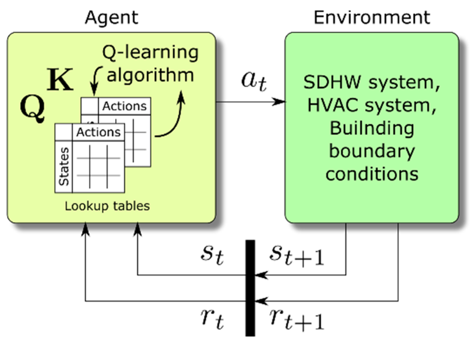
15]. The RL approach is based on the interaction between an agent and his environment (
Figure 1). The agent is something that can see the status or configuration (
) of the environment and that can perform actions (
) to change it. Moreover, upon application of an action, the agent receives from the environment an evaluative feedback signal. This signal is called reinforcement and can be a reward or a punishment. All the actions that the agent applies have an impact on the environment, and the agent learning process is influenced by the environment through the rewards.
The objective of the whole learning process is to find the optimal policy to perform whatever task the agent is supposed to carry out. The optimal policy is defined as the one that maximizes the cumulative reward (or the expected cumulative reward) given by the environment. This is achieved by mapping states (configurations) to actions and modifying that mapping until the optimum is encountered.
The RL technique used in this paper, where an agent learns a policy to maximize an objective function, is based only on the current and next state of the system,
and
, respectively, without using prior history. This approach is justified because the reward depends only on the current state and current action. Normally RL problems are modelled in the framework of Markov decision processes (MDP), that is stochastic processes where the probability of transition from one state to the next one depends only on the actual state, although a deterministic formulation of the method can be given [
16].
To implement a self-optimizing controller for the reference system, a particular RL algorithm called Q-Learning, originally developed in Reference [
17], was applied. This algorithm belongs to the class of unsupervised, model-free RL methods. Here the agent does not have any prior knowledge or model of the system characteristics from which it could estimate the next possible state. Essentially, the agent does not know what the effects on the environment of a certain action are and chooses the next action on the basis of the cumulative effect of the actions performed in the past.
All reinforced learning problems are solved by applying the dynamic programming paradigm to the so-called value function, which is usually defined as a weighted sum of the rewards received by the agent. Model-free methods need to find both the value function and the optimal policy from observed data. Q-learning solves this problem by introducing an evaluation function representing the total cumulative reward obtainable if an action is carried out in a certain state and then the optimal policy is followed afterwards. The value of this function indicates how good is to perform action in state .
For practical application, it is reasonable to assume that the number of states describing the environment and the number of actions that the agent can perform are both limited. Then, the Q-learning algorithm calculates the
function iteratively, storing it in a lookup table
(
Figure 1). During the learning phase, the agent updates the values of the
matrix (initialised to zero) at each step according to the well-known Equation (1):
where α is the learning rate and γ is the discount factor and both take values in the [0,1] interval. These two factors weight, respectively, the increment to the present Q-value (learning speed) and the contribution from the future states (decay or discount). The value multiplied by factor α is also known as the temporal difference error [
15]. In this application, a one-step backup method was used. In this method, the matrix
is updated using the value observed only in the next state [
17] and
represents the reward returned by the environment in the step analysed. Often, the reward is a value from a finite, conventionally defined set such as {100, 0, −100}. In this investigation, we opted to directly link the reward to the energetic performance of the control—essentially the objective function. Details on how the reward is calculated will be given in
Section 3.3.
One of the main RL challenges is finding the correct trade-off between the so-called exploration and exploitation phases [
15]. The trade-off arises because in order to choose the optimal action in every state, the agent has first to discover what the cumulative effect of the actions is, which can be done only by choosing an action with the purpose of exploring the environment, something that most of the time is far from being optimal from the reward point of view.
One of the simplest local methods for the exploration applied in the literature is the ε-greedy method [
15]. Following this method, the next action a
t is selected following two alternative strategies chose randomly. The selection is governed by the ε parameter, which can be set constant throughout or decreasing during the learning process. The action is then chosen through a uniform random selection with probability
and using the Q-learning method otherwise. This is described by Equation (2), where
is a uniform random variable on the interval [0,1].
Normally, the algorithm is stopped when a sort of global convergence indicator reaches a threshold. In the application described in this paper, instead, the learning algorithm goes from exploration to full exploitation using an alternative local method. Unexpected difficulties have indeed been found with the convergence speed of the ε-greedy implementation, which is particularly critical in this type of application. This will be discussed in detail in
Section 2.1.
1.3. Traditional Control of Solar Systems
In their dissertations, Kaltschmitt [
18] and Kalogirou [
19] show how to control two different kinds of solar thermal systems, named Low-Flow and High-Flow, by simply switching on and off the solar circulation pump depending on the differential temperature between the collectors and the thermal storage. They also give some indication of the impact of the pump electrical consumption in relation to the heat available at the outlet of the solar installation. Streicher in [
20] analyses different schemes of solar thermal systems with internal and external heat exchange and the effect of these characteristics on the behaviour of the whole system.
Badescu [
21] studied the optimal flow control for a solar domestic hot water (SDHW) system with a closed loop flat plate collector system, using two levels of constant mass flows in the systems. For an open loop, the same author [
22] finds the optimal flow in order to maximize the exergy extraction from a solar thermal system for DHW. Different strategies for flat-plate collector operation are reported in Reference [
23]. Here, the best strategy to optimize the efficiency of the collectors is applying a constant inlet temperature control (to allow simple connection with other systems) when flow-rate control is not possible (best at 7.8 L/hm
2). For applications where a set point temperature is required as a collector output, the control of the mass flow-rate (with a max of 7.8 L/hm
2) gives the best performance in terms of useful energy and collector efficiency.
As reported in Reference [
22], different control studies were carried out in the past with the optimization of different objective functions. Kovalik and Lesse [
24] and Bejan and Schultz [
25] studied the optimization of the mass-flow rate for a solar system and for heating or cooling an object, respectively, as well as Hollands and Brunger [
26] who studied the flow optimization for a closed loop system. Additional comments could be found in De Winter [
27]. In a recent study, Park [
28] briefly analysed the behaviour of the numerical model of a solar thermal installation in Korea regulating the mass flow in relation to the collector’s area when the state of the system was not observable.
A deep analysis of the effect of mass flow on the collectors of small and large SDHW systems is reported in Furbo [
29]. For small SDHW systems, the greatest performance is claimed at a flow rate from 12 to 18 L/hm² for combi-tank systems and 18 to 24 L/hm² for preheating systems. Moreover, analysis of the performance of these systems are reported when the mass flow control is based on the temperature difference (ΔT between the collector’s output and the bottom of the storage
m’ = 1.5* ΔT (L/hm²)) or on the global radiation on the collectors (G (W/m²), resulting in
m’ = 0.6 × G
0.5 (L/hm²)). These two approaches show an increase in the thermal performance of the system, with respect to the reference case, by 0.9% and 0.8%, respectively. For large scale plants (20–50 m
2; 1–2.4 m
3) two systems were analysed: a low-flow system with a mantel tank and a system made of a spiral tank or storage equipped with external exchanger. Also, this class of systems was analysed to understand the effect of different control strategies.
1.4. Applications of Fuzzy Control to Solar Thermal Systems
In their review of the control techniques concerning buildings integrated with thermal energy storages, Yu et al. cite a work where fuzzy control is used in a peak-shaving controller [
30]. Their comments about the feasibility of such type of control for solar thermal systems are in line with those of Camacho [
31,
32], where the usefulness of a fuzzy controller is ascribed to its ability to deal with nonlinear or complex behaviours. Compared with other thermal systems, where the availability of the energy source is under control of the plant operating agent, in solar plants, the availability of the primary energy source cannot be manipulated, and it is stochastic in nature. The position of the sun, the intensity of direct and diffuse solar radiation modified by cloud cover in addition to components like storage, thermal machines, and heat exchangers that are traditionally part of solar thermal applications heavily affect the dynamic behaviour of such systems. Salvador and Grieu [
33] give an example of how fuzzy logic can be used to model occupancy in an optimization problem regarding the impact of thermal loads such systems and the power grid.
An exhaustive paper written by Kalogirou [
34] presents the application of artificial intelligence techniques to solar energy applications. Here, after an introduction of artificial intelligence techniques, their application to solar systems are listed. Concerning fuzzy controllers, only a selection of the most significant control strategies are reported here. The first one regards a fuzzy controller predicting the internal air temperature used to manage the house heating system [
35]. The others, due to Lygouras [
36,
37], regard the application of fuzzy control and its comparison with a traditional PID control to a solar cooling air conditioning system using two different approaches. An adaptive fuzzy algorithm for a specific domestic hot water system (instantaneous boiler) was proposed by Haissing and Wössner [
38]. The motivations behind their approach are the same as this paper, although the purposes are different: there, the optimization of a PID controller was performed, and here, the energetic aspects of the application were considered.
1.5. Applications of Reinforced Learning to Energy Systems
Many applications of RL in the fields of combinatorial search and optimization process like board games, industrial process control, manufacturing, robotics, and power systems appeared in the literature over the past years. Focusing on energy systems, an application of RL to the automatic generation control (AGC) of a power system is reported in References [
39,
40], where the performance of an RL algorithm is compared with that of a properly designed linear controller. The paper underlines the potential of the method related to the flexibility in specifying the control objective before the learning phase. Other applications in this field are reported in the PhD thesis of Jasmin [
41], focused on the application of RL for solving the power scheduling problem.
Regarding the application of RL to thermal systems, Anderson [
42] presents a comparison between the different control strategies for a heating coil in a simulated domain. Here, the RL is combined with a PI controller to reduce the error of the controlled variable over the time. The result of this combination shows, after an opportune training phase, a reduction of the root mean square error compared with the simple PI controller. Reinforced learning is also covered in the review by Yu et al. [
30] cited above.
A couple of papers by Dalamagkidis and Kolokotsa [
43,
44] present an implementation of RL using a temporal difference (TD) error method for optimising the thermal comfort control of commercial buildings without requiring an environment model. In these works, the authors coupled the RL with a recursive least squares method to increase the method convergence speed. In Reference [
43], in particular, the authors show the use of a reward composed of different parameters, properly weighted, in order to minimise the energy consumption while maximising, at the same time, the comfort and air quality. The state of the system is related to the internal and external temperature and the actions are related to the operation of the heat pump, the compression chilling system or the automatically opening windows function. One of the issues underlined from the authors is the lack of scientific contributions related to the application of this methodology to internal comfort control; therefore, the choice of the reinforcement learning parameters was made on the experience and test effectuated on the system. Moreover, the authors stress the importance of the reward mechanism in the learning process and this topic will be addressed with future development. Finally, it is claimed that the environmental inertia must be deeply analysed in order to understand the time response of the environment and correctly compute its effect in the learning analysis. Concerning the energy efficiency of next generation buildings, the papers of Yang et al. [
45] and Kim and Lim [
46] give details on how the power consumption can be reduced utilising the Q-learning algorithm. Both papers provide details on how the state space is constructed and employ a stochastic framework for the problem formulation. Yang et al. [
44] is very effective in describing the problem, the demo case, the theoretical references, and the details of the implementations. Moreover, it deals with the curse of dimensionality by coupling Q-learning with artificial neural networks. In Yang et al. [
44], the benefits are a result of the combination of reinforced learning and the solution for an optimization problem, while Kim and Lim [
45] solve the optimization problem implicitly using the Q-learning algorithm itself. Both papers are relevant to this work, although here the scope is narrower: not the building but the solar DHW system alone. Kazmi et al. [
47] proposed a solution for this problem employing a set of tools including a hybrid reinforcement learning process, seasonal auto-regressive integrated mobile average (SARIMA) model, and a hybrid ant-colony optimization (hACO) algorithm. The paper contains useful remarks about thermal energy storage modelling.
In a two-paper work, Liu and Henze [
48,
49] present the RL application to the optimal control of building passive and active systems. In particular, a thermal passive system is controlled in order to minimize the energy consumption of the heating and cooling system installed in a commercial test structure. In this work, an interesting hybrid approach is presented based on two different phases: the simulated learning phase and the implemented learning phase. This idea came from the knowledge that the RL method for control gives near optimal results compared with the optimal control strategy based on predictive control, but takes an unacceptably long time during the learning phase. Starting from these premises, the hybrid approach was developed to combine the positive features of both the model-based and the RL approach. In this way, in the first learning phase, the agent is trained using a model of the system followed by a refined learning phase (or tuning phase) when the agent finalises the learning phase in direct connection with the real system.
In a previous work, Henze [
50] showed how to generate an increase in the peak savings and a reduction of the costs for the same class of problems (related to the charging and discharging phases control of a cool thermal storage system) using a model-free RL to optimize the control. Henze points out that the RL controller does not reach the best performance of a model-based predictive optimal control but shows a favourable comparison with conventional control strategies for cooling. Furthermore, the RL approach allows, using past experience and actual exploration, to account for the non-stationary features of the physical environment related to seasonal changes and natural degradation. An example application of RL techniques can be found in Reference [
51], where the authors present a model-based RL algorithm to optimize the energy efficiency of hot water production systems. The authors make use of an ensemble of deep neural networks to approximate the transition function and get estimates of the current state uncertainty.
1.6. Joint Applications of FC and RL
Several applications where FC and some sort of learning or self-tuning procedures are applied synergistically have been found. However, this synergy does not seem to be often exploited in energy systems. A few non-exhaustive examples of the joint application of the two techniques are: the optimization of the data traffic in a wireless network [
52]; the tuning of a fuzzy navigation system for small robots [
53]; the robust control of robotic manipulators [
54]; and the PI and PD controllers’ tuning [
55,
56]. All these papers refer to an adaptation of the Q-learning algorithm called Fuzzy Q-learning [
57,
58]. Kofinas et al. [
59] applied this algorithm also to manage energy flows in micro-grids. Other applications where fuzzy logic is coupled to other self-learning approaches are: Reference [
60], where actor–critic learning, neural networks, and fuzzy inference mechanism are used to design an adaptive goal-regulation mechanism for future manufacturing systems; Reference [
61], where RL and the adaptive neural fuzzy inference system (ANFIS) are used to implement a non-arbitrage algorithmic trading system; the inspiring work of Onieva et al. [
62], where an on-line learning procedure is implemented to adapt the number and shape of input linguistic terms and the position of the output singletons of a vehicle cruise control system FC; and Reference [
63], where an iterative procedure called iterative learning tuning, based on minimization of a cost function, is used to tune the singletons output membership functions of a monocycle controller. Integration of reinforced learning and fuzzy logic at high level is found in the work of Haber et al. [
64], where these techniques are used to demonstrate the feasibility of what is called artificial cognitive control architecture. The paper describes the design of the architecture and its implementation to an industrial micro-drilling process. The work is an excellent example of how the tools and concept of theoretical computer science and cognitive sciences can be applied to the control of complex industrial systems. Details about the design of the reinforced learning component of the cognitive controller are found in the Reference [
65].
In the field of energy systems for buildings, an interesting work by Yu and Dexter [
66] appeared, where the authors present the application of RL to tune a supervisory fuzzy controller for a low-energy building. In this work, the authors showed an application of online learning scheme based on pre-generated fuzzy rule-based. Here, the learning process is accelerated with the use of the Q(λ) algorithm with a fuzzy state variable and eligibility traceback. The successful application of RL to the supervisory control of buildings is strongly dependent on reducing the state space and action space of the controller. As reported in other papers, the importance of off-line learning is underlined, included in this case in the knowledge used to devise the fuzzy controller rules. The approach based solely on the online learning takes an unacceptably long training time.
The above discussion suggests that despite its potentiality, the application of an FL control and RL to thermal energy systems is lacking (
Table 1). It seems, therefore, reasonable to investigate their application to this type of system.
2. Methods and Performance Figures
The typical cycle time of digital controllers employed in solar thermal systems ranges from about a few seconds to several minutes. This is quite large compared to other industrial fields (e.g., power electronics, robotics) where the cycle time can be more than three orders of magnitude smaller. This is a consequence of the small value of the thermal diffusivity and long transport delays of such systems, which limits their bandwidth and makes them more difficult to control. Often, it takes several seconds to see the effect of an action, such as the activation of a circulator, on the temperature measurements. Of course, the slower the controller, the fewer data per the unit of time are available for exploration, making the Q-learning algorithm slower to understand how the environment responds to exogenous stimuli.
The size of the state-space representing the system, i.e., the size of the so-called
matrix, has obviously a great impact on the convergence time of the algorithm. In fact, the larger the state-space and the number of possible actions, the longer it takes to explore. This is particularly true when the state-space describing the system is multi-dimensional and continuous. Such state spaces need to be discretized with caution (due to the curse of dimensionality) before applying any reinforcement learning algorithm [
67,
68].
These are major challenges to the development of self-learning controllers for solar thermal systems which are naturally described by continuous variables (temperature, pressure, flow) and face daily and yearly seasonality. Obviously, a controller taking several years to find the optimal policy does not sound so smart to the potential customer. In the test case, the state space was obtained by discretizing the Cartesian product of two continuous variables.
2.1. Q-Learning with Guided Exploration
The application of the standard ε-greedy Q-learning algorithm to the test case described in
Section 2.4 required modifications to overcome a problem during the explorative iterations.
Being that the number of explorative actions was relatively low and the number of trials quite small in the present application, there was no guarantee that the pseudo-random generator would distribute the various actions evenly across the action space within a reasonable time. This can lead to runs where some points of the state–action matrix are not visited for long times. In order to overcome this limitation, a guided exploration algorithm was implemented in place of the random ε-greedy approach. The idea is to explore, at each step, the action whose outcome is less known until a sufficient number of explorations has been performed. To implement this idea, a second matrix was introduced. . has the same dimensions as ( rows and columns) and contains the number of times each state–action pair has been visited up to the current time-step. Given a certain state, the new action is selected evaluating the minimum of the matrix along the row corresponding to that state, until a minimum number of trials per action () is performed. In this way, the exploration of each action is ensured in a minimal number of trials. Moreover, if some states are visited more frequently than others, they reach convergence before those visited less frequently. This means that after a state reaches convergence, in that state the following actions are chosen purely based on the Q-value. In this paper, this is called a local convergence criterion because the transition from the exploration to the exploitation phase was evaluated for each state independently.
To understand how this was achieved in detail, the vector
is introduced. For every state
,
is defined to be 1 when the sum of the numbers in the row of
referring to state
is greater than
and 0 otherwise. This is concisely expressed by Equation (3).
The action to be performed at time
is then selected by means of Equation (4) instead of Equation (2).
In either case, matrix
is updated by incrementing the entry referring to the current state
and the so selected action
, like in Equation (5),
while matrix
is update with Equation (1) as usual. From how the
matrix is updated, it follows that
is equal to one if and only if the state
has been fully explored, that is all the actions in state
have been tried out at least an
number of times.
The vector
is used to define a convergence criterion for the RL algorithm. Considering that
always holds (with
at the beginning of the exploration phase and
at the end), the
exploration factor can be defined (Equation (6)).
This parameter indicates the percentage of the matrix explored, and consequently the progress of the learning process toward its end.
The RL algorithm is also beneficial for tracking an evolution in the behaviour of the system (or more generally the environment), e.g., due to ageing of components or to the time variance of its boundary conditions. In these circumstances, the agent should be able to recognize the new distribution of the optimal actions to do. However, making an analogy with the human learning process, this can be as difficult as trying to correct a bad habit (or “wrong learning”). If an output pattern or a sequence of events has been tried a lot of time, it brings with itself an experience (the data stored in the and matrices) that is difficult to discard when the optimal policy changes. Moreover, in the adapted algorithm the exploration phase stops when a state is fully explored.
2.2. Partial Reset of Stored Information
To overcome these limitations, the
and
matrices are periodically reset by partially discarding the information therein stored. To clarify this point, it is understood that the information is
totally discarded when the two matrices are reset to zero. In this way, all the information that the system has gained in the previous period is forgotten and the algorithm restarts from arbitrary initial conditions. Totally discarding the accumulated knowledge is, however, not adequate for tracking slow changes of the system parameters such as fouling. Thus, a “partial discard” is more useful. The information in the two matrices is said to be
partially discarded when the new matrices in the learning are computed as:
The parameters and ( in the following) span between 0 and 1 and are understood as a sort of “exploration degree” when a new explorative phase is started. represents a matrix the same size as . and composed entirely by identity elements. When the RL agent updates the matrices with Equation (7), a new exploration phase with a duration depending on the selected parameter is started.
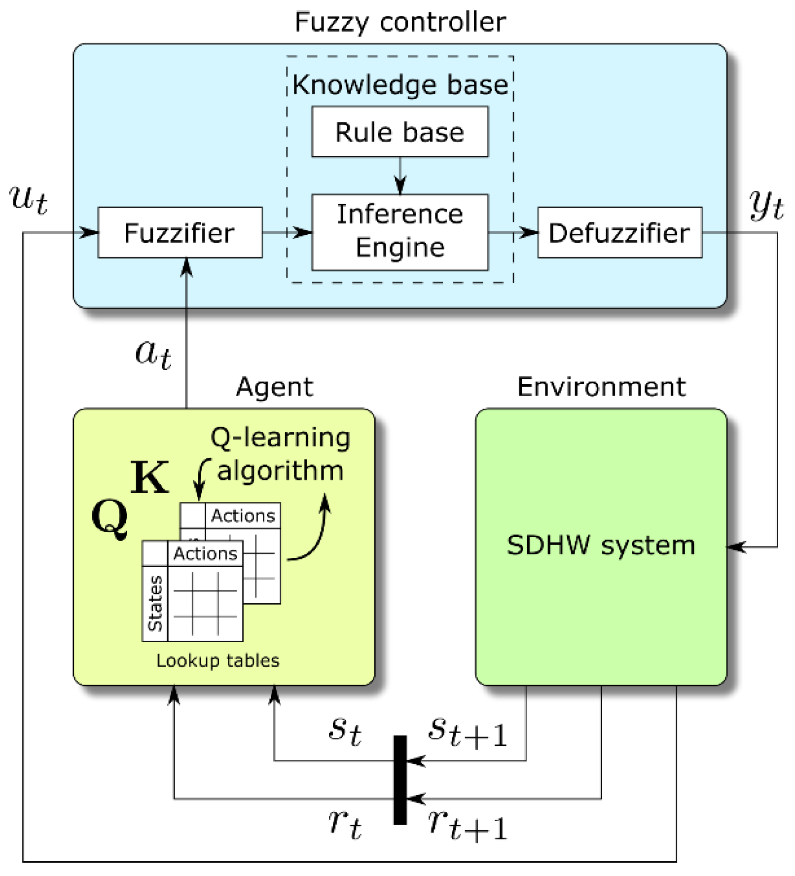
2.3. Coupling between FC and RL
Two aspects motivate the coupling of the Q-learning algorithm with a fuzzy logic controller. The first one is the easiness with which complex controls can be designed and modified using fuzzy logic. The second one is their intrinsic ability to approximate and discretize functions [
69]. Essentially, the FC is designed as a function of a limited input quantity (solar irradiation)
x to a limited output quantity (circulator command)
y. The input quantity is transformed into a linguistic variable by using the linguistic values “low”, “medium”, and “high”. A similar transformation is used for the output quantity. The rule base embedded in the inference engine represents the identity and is not subject to change. The RL is coupled to this FC by changing the definitions (in terms of membership functions) of the input linguistic values, i.e., the actions made by the Q-learning agent are performed directly on the FC fuzzifier (
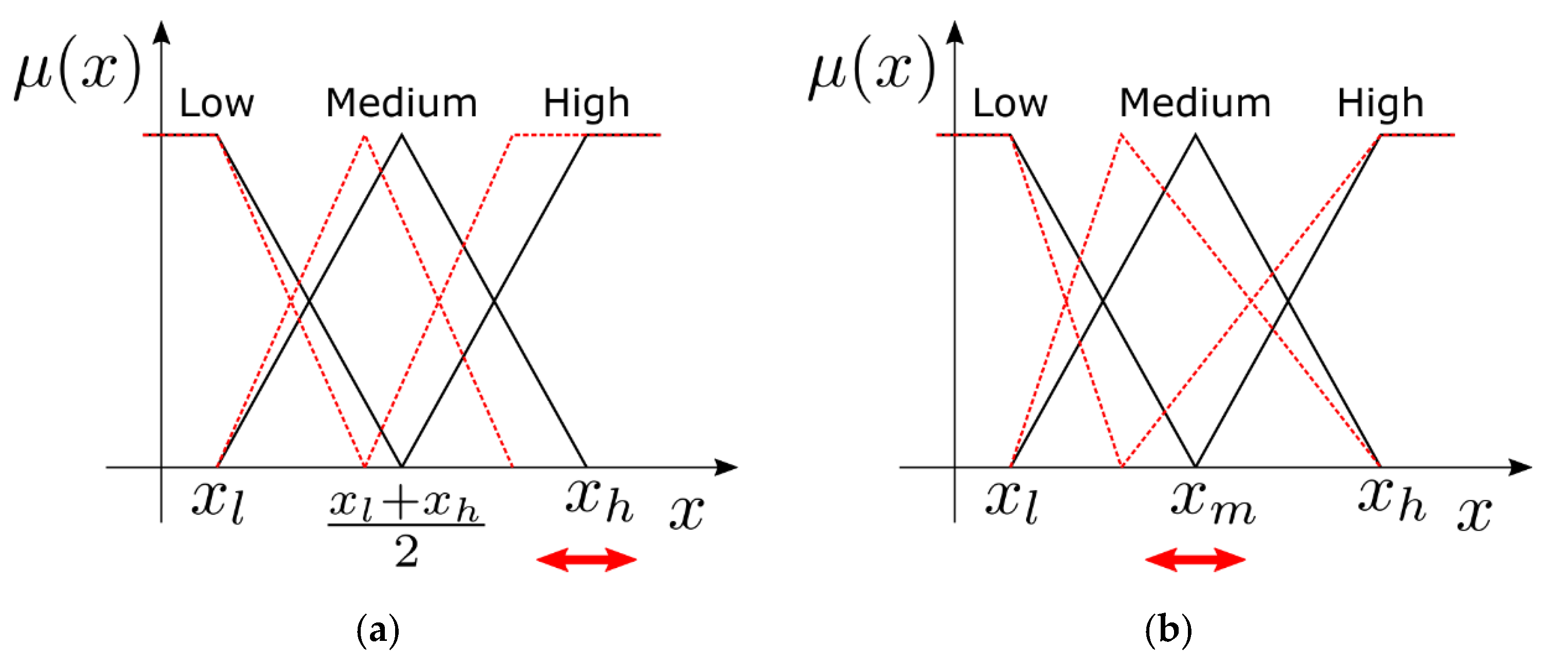
Figure 2).
Two ways to perform the coupling were considered: changing the position of the peak of the “high” linguistic value and changing the position of the “medium” linguistic value.
Figure 3a,b clarifies how the membership functions were modified by a change of the controlled parameters in the two cases.
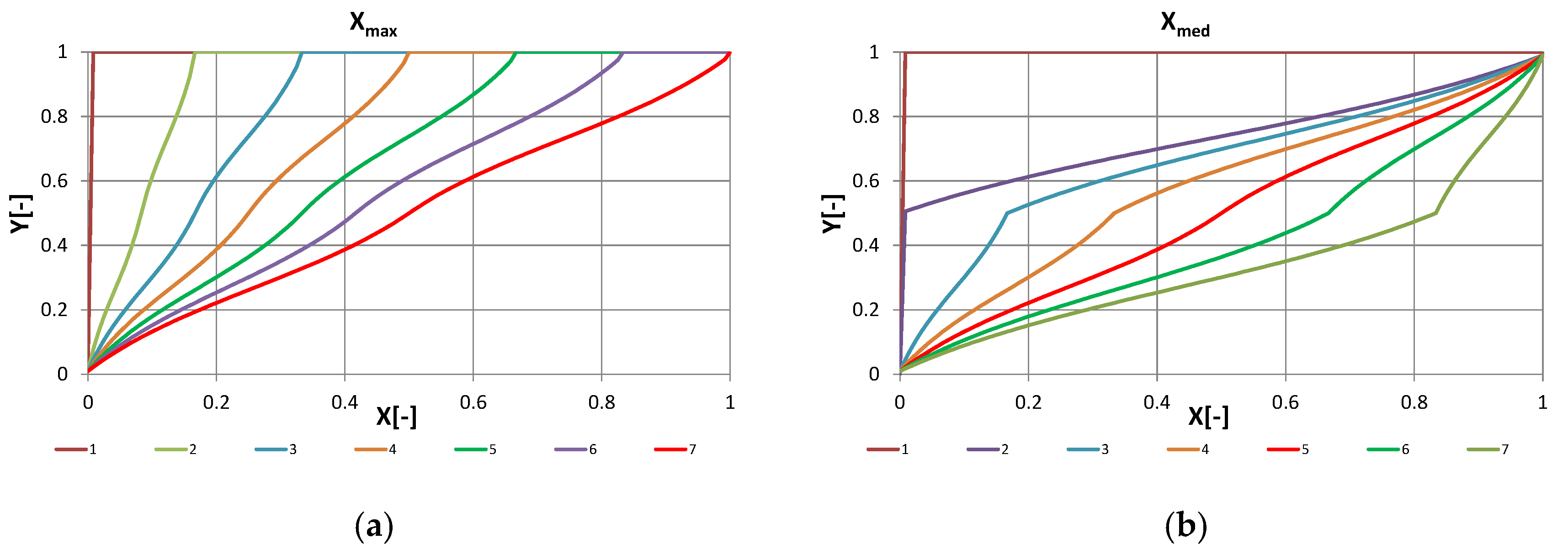
Figure 4a,b shows the resulting input–output mappings under seven different values of the control parameter.
The action performed by the RL is the selection of the trans-characteristic to be in the next period. In the first case, this is like changing the control gain used in the circulator control.
This arrangement allowed us to come up with a controller with a relatively small state-space (693 states) and a behaviour not too far from those used in experimental practice (control proportional to the solar irradiation).
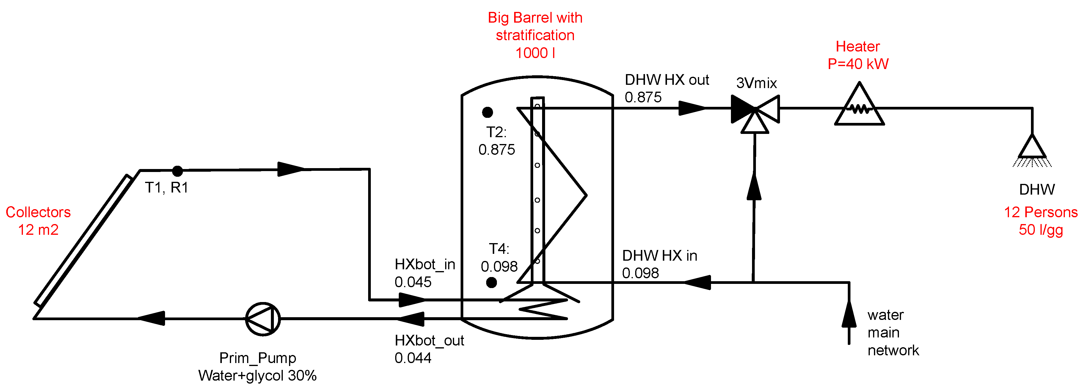
2.4. System Description
As an application example of the methodology explained previously, a simple traditional solar thermal system for domestic hot water (SDHW) was considered. A Trnsys model of such system was developed to understand the effect of different control strategies. The design and components sizing was made starting from the thermal storage because the numerical model of this component [
70] was validated using monitoring data from a SolarCombi+ installation [
71] following the procedure reported in Reference [
72].
The thermal storage consists of a 1 m
3 water container with two internal heat exchangers, one for the solar primary loop and one for the domestic water loop, as shown in
Figure 5. A stratifying storage was employed to take advantage of the increased heat exchange between the stored water and the DHW heat exchanger due to the stratification of the temperature inside the storage. It was assumed that a mixture of water and propylene glycol (30% in volume) was present in the primary loop to avoid freezing during winter seasons. A collectors area of 12 m
2 was adopted using standard design rules of thumbs of solar thermal systems for DHW [
20]. The DHW request profile was computed using DHWcalc [
73,
74] considering a multi-family house with a daily consumption of 50 L/gg per person and three families composed of four persons each. An electrical backup system was considered to fulfil the energy demand reaching the DHW set temperature of 40 °C when not enough solar energy was harvested and stored in the tank. The configuration with two heat exchangers was used also to avoid problems with bacteria from the
Legionella genus [
20].
2.5. Performance Figures
Some figures of merit were used for the evaluation of the system’s thermal performance and the variation of the behaviour using different control logics.
Collectors’ efficiency “
”: the ratio of the energy collected in the reference period (
= {year, month}) by the solar system over the energy that hits the collectors.
Gross solar yield “GSY”: represents the energy captured from the solar field per square meter of collectors. Like the efficiency, this parameter shows how efficiently the collectors do their work.
Seasonal performance factor of the primary circuit “SPF
coll”: a seasonal index obtained by forming the ratio of the thermal energy collected by the system over the electrical energy consumed by the circulation pump of the solar circuit.
Seasonal performance factor of system “SPF
dhw”: the ratio of the thermal energy used to cover the DHW demand over the total electrical energy employed for fulfilling this demand. The total electrical demand is composed of the consumption of the auxiliary electrical heater and the electrical energy consumed by the circulation pump of the solar circuit (
).
The global radiation on the collectors’ plane “
”: simply the integral of the global irradiance
.
Lost heat for control purposes
: a parameter quantifying the inconvenient situation where the difference between the inlet and outlet temperature of the internal heat exchanger is negative, which may happen during the initial phases of the system start-up or in the evenings.
3. Results Discussion
3.1. Base Cases
As mentioned in the introduction, solar DHW systems are traditionally controlled using the temperature difference between the fluid in the collectors and in the thermal storage. More evolved systems take into account a minimum radiation at which the system is switched on, and as reported in Ref. [
29], the control signal of the pump can be a function of the radiation itself. Therefore, four different control strategies were applied to this system in order to form a solid base of reference cases:
Control of the primary pump based on the temperature difference between the collectors and the thermal storage (DT) using a hysteresis with fixed values (2–7 °C);
Control of the primary pump based on the global irradiance using a hysteresis with fixed values (100–150 W/m2);
A combination of controls A and B. The A controller is qualified by the output of the hysteresis of the B controller;
Control C where the primary pump modulates the mass flow as a function of the radiation (linear modulation with the maximum at 600 W/m2).
In all the above cases, a further control on the maximum temperature allowed in the storage has been implemented to avoid overheating and stagnation problems in the solar circuit during simulations.
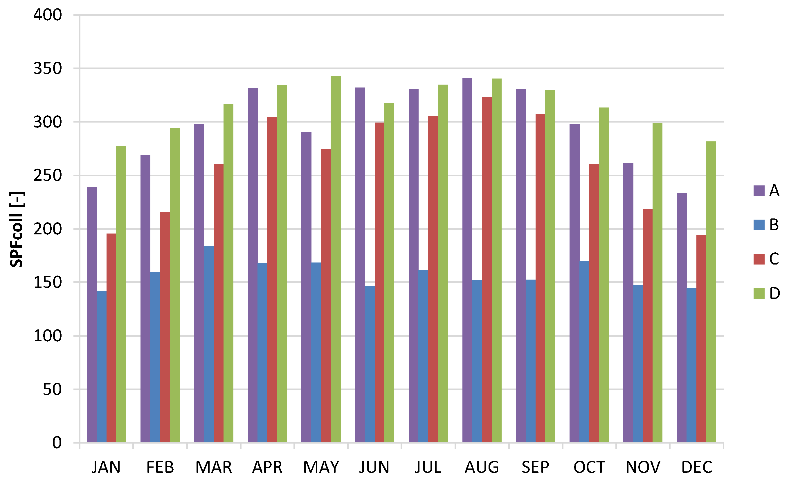
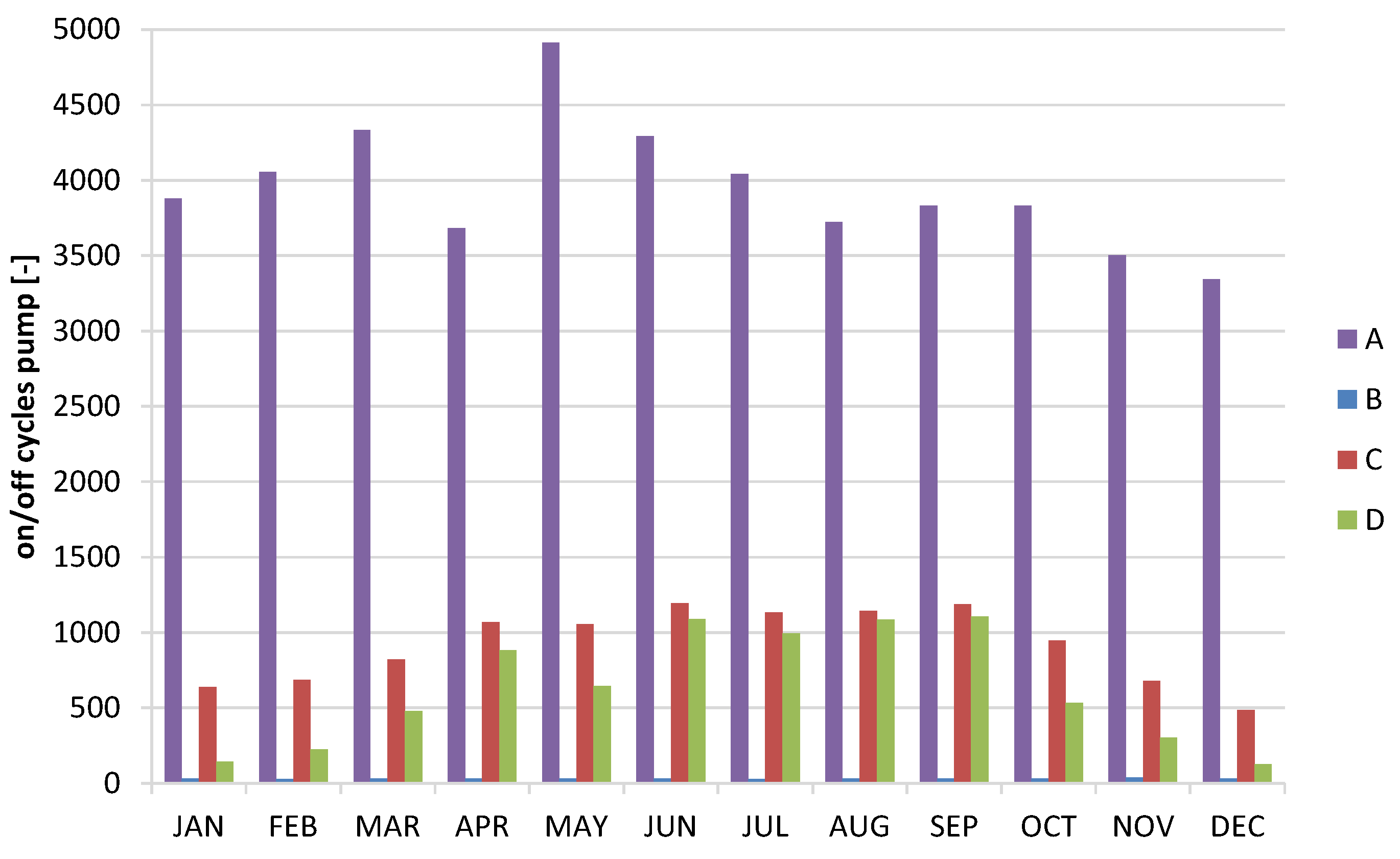
Table 2 compares the yearly performance of the four control strategies using the performance figures introduced above, while
Figure 6 and
Figure 7 graph the monthly performance. The SPF
coll increases from case B, to cases A, C, and D mainly for the use of a control strategy based on two parameters (radiation and temperature) that allows a reduction of the thermal losses and the electrical consumption of the pump. The best SPF
coll performance was achieved in case “D” where the control of temperature, radiation, and the modulation of the pump (as a function of the radiation) were adopted. From the system point of view, the best performance in terms of SPF
DHW was achieved when the losses (reversed energy flow) were minimized using the DT control and temperatures in the storage were maximized, reducing the usage of electrical backup (case “C”). In this case, however, the number of times the circulator was switched on and off was higher, as clearly shown by the monthly profiles reported in
Figure 7.
Increasing the hysteresis controlling the temperature difference in the cases A, C, and D (from 2–7 °C to 2–14 °C) allows decreasing the number of on/off cycles with a limited impact on the performance. A slight increase of SPFcoll can be observed in case C and D and a slight decrease in case A, all between 2.5% and 7.5%. The situation was opposite for SPFdhw, where a slight increase in case A and a slight decrease in cases C and D was observed. The number of on/off cycles, however, remained elevated, between 5200 and 7200 per year.
3.2. Fuzzy Logic Controller
The development of a fuzzy–based reinforcing learning algorithm was seen as a way to attain good performance both in terms of SPF and in terms of on/off cycles. Reducing on/off cycles to a minimum can have a great impact on the expected life of circulators, increasing it significantly.
The fuzzy controller was designed starting from the logic of case B where the independent quantity was the solar irradiance and the control variable the circulator speed. As mentioned in
Section 2.3, the linguistic terms “low”, “medium”, and “high” were implemented with three triangular membership functions centred at about 0, 600, and 1200 W/m
2, respectively. The output membership functions were defined in the same way, with three triangular membership functions, equally distributed on the universe of discourse of the control parameter (between 0 and 1). The method used for the defuzzification phase was the centre of area [
11,
66] and three rules were defined that related the three membership functions on the input with three membership functions on the output (low radiation with low speed, medium radiation with medium speed, and high radiation with high speed).
In order to assess the robustness of the controller and to provide a connection to the RL algorithm, the FC controller was implemented with two different parametrizations of the input linguistic terms. In the first one, denoted by letter H, the membership functions were parameterized by the “high” radiation peak. In the second one, denoted by letter M, the parameterization was done by the “medium” peak. The two families of membership functions are shown in
Figure 4, while the resulting control characteristics are shown in
Figure 5. In the following tables, the yearly results of the H-FC are reported in
Table 3, while those of the M-FC are reported in
Table 4.
A higher level of SPF
coll can be reached with the “medium” radiation setup, although this is attained decreasing the electrical consumption of the pump at the expanses of the captured solar energy (GSY). The “high” radiation setup, instead, achieved the maximum values in terms of SPF
dhw. Monthly data of SPF
coll for the H-FC case were also reported in
Figure 8 with different lines for seven different values of the parameter defining the family, from 0 to 1200 W/m
2. To ease comparison with the previous four control strategies shown in
Figure 4, its bars were re-plotted in the background of this figure. Looking at this graph, the big difference notable is between case D and the FC with the action a7 (high radiation imposed at 1200 W/m
2) that allows to reach the best performance in terms of SPF
coll.
3.3. Reinforced Learning Controller
The RL was applied to both cases of FC introduced above by means of the modified Q-learning algorithm described in
Section 2.1. The RL and FC parts were connected, as described in
Section 2.3, because the learning agent (controller) can choose which membership function to employ in the FC. This resulted in the selection of one out of seven characteristic functions (shown in
Figure 5 left or right) to be used in the real-time control for the entire period
between two iterations of the Q-learning algorithm.
The definition of the state-space variables for the application of RL techniques was performed, trying to minimize the number of states, and therefore, the number of variables involved. Two parameters were identified as essential to describe the system dynamics: the solar radiation at the collectors and the temperature of the storage. Since no reference was found in literature covering the discretization of the state-space in such an application, the following arbitrary choices were made:
The average temperature of the storage was modelled with nine intervals of 10 °C each from 0 to 90 °C;
The radiation on the collectors’ plane was modelled with 11 intervals of 100 W/m2 each from 0 to 1100 W/m2.
The Cartesian product of these two grids represents the Q-learning algorithm state-space. The elements of such space were ordered and rearranged as a vector to be addressed linearly. This vector had a total of
components. The size of the action space was
, as there were seven curves in each FC family to be selected from. The period of the Q-learning iteration
was set to 5 min down from the initial 15 min which were initially considered in order to reduce the algorithm convergence time. The parameters affecting the implemented Q-learning algorithm are summarized in the following
Table 5.
The objective of this work was to compare the performance of the coupled RL and FC controller with the reference cases. In particular, the SPFcoll indicator was considered because it is directly influenced by the variables selected to construct the Q-learning state space. The SPFdhw is somewhat more relevant from the economic point of view but it is influenced by a variable (the DHW draws) which is not in the selected state-space, and therefore, the algorithm cannot learn anything about it.
The reward function was defined assuming that rewards proportional to the current value of the quantity to maximise (SPF
coll) results in the actual maximization of that quantity. A preliminary analysis used a reward equal to SPF
coll measured on the
interval, but simulations showed that the learning was not effective, and the best performance of the reference cases could not be achieved. The following additive form of the SPF
coll has proven to give better results than using directly its fractional form (10):
3.4. Coupled RL and FC Simulations Outcomes
The results of two simulations of the coupled control algorithm spanning 5 years are shown in
Table 6. The first five rows refer to the H parametrization, while the successive five rows refer to the M parametrization. In either case, after the second year, the SPF
coll value gets close to the maximum attained by the reference cases (
Table 2 and
Table 3).
Figure 9 shows a clear difference between the first and the second year of the monthly profile of the performance indicator for the five years of learning (reported also in the first five rows of
Table 6), while in the following years, the values are close to each other. Most of the learning phase happens during the first seven months of the first year.
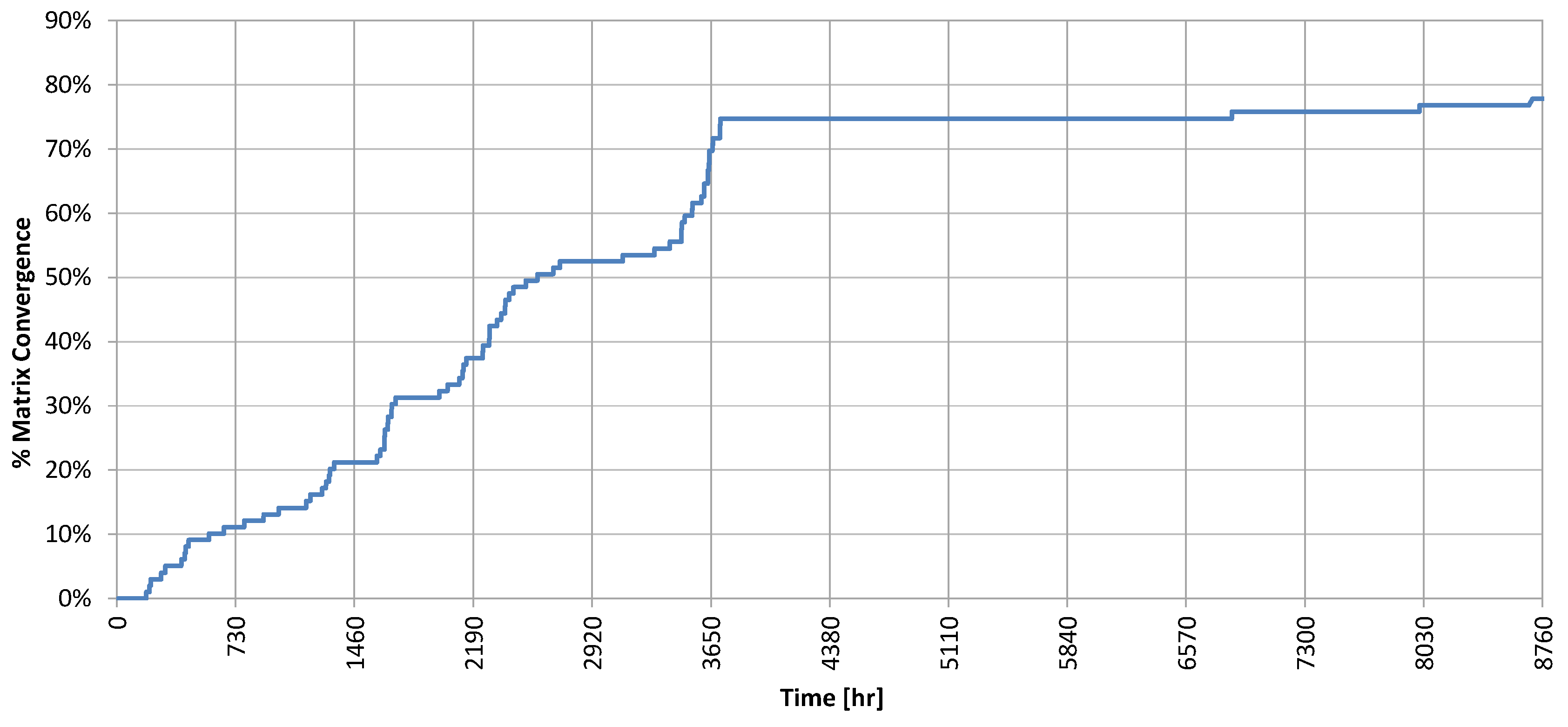
This was confirmed by the exploration factor (
) reported in
Figure 10. It becomes apparent why the performance profile did not change significantly after the first year: the maximum of the exploration factor was reached within this time (in fact the first five months), meaning that what the Q-learning had to learn about the system, it had learnt it within this time. Minor increments in the following seven months were due to states visited rarely during the normal operation of the system. The reader may wonder why the exploration factor did not reach 100% after enough time. This was unavoidable and happens because some states (for example, a temperature of the storage less than 10 °C with a level of radiation higher that 900 W/m
2) were not reachable, and therefore, never explored.
Different simulation runs were performed increasing the Q-learning cycle time , the minimum number of events , and the total number of states (by discretizing more). In all cases, the duration of the explorative phase increases, and therefore, so does the time required to reach convergence, while the final performance of the controller does not change substantially.
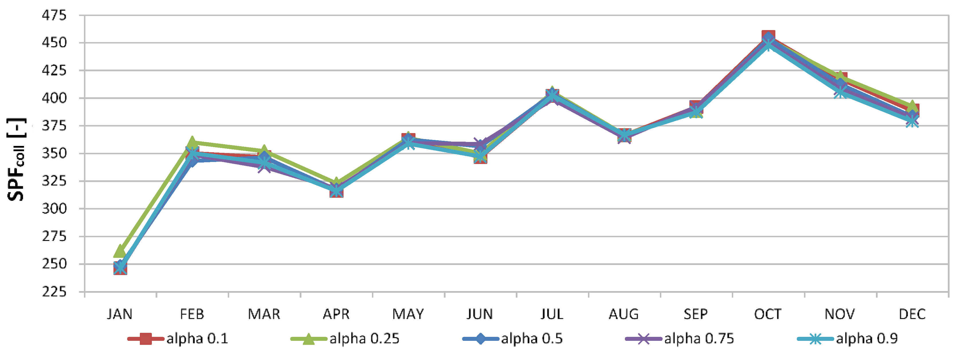
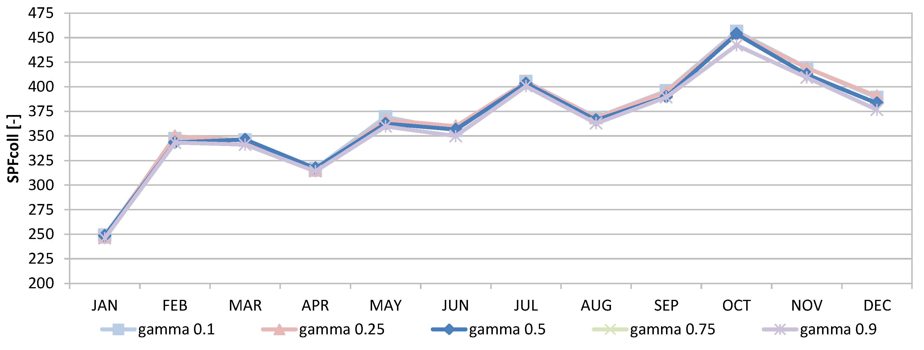
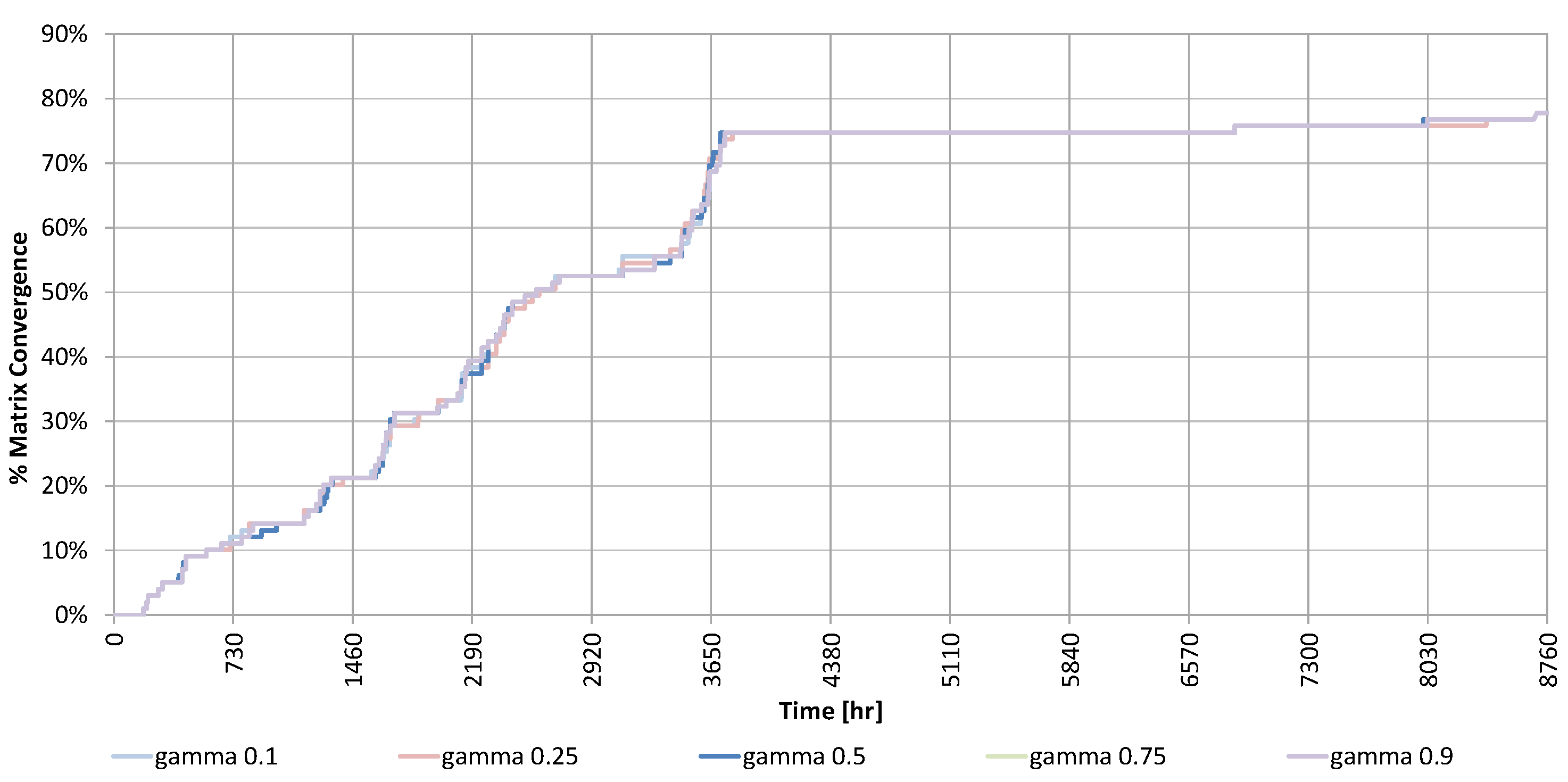
For the H-FC case, further simulation runs were performed varying the learning factor
and the discount factor
.
Figure 11 and
Figure 12 show the deviations in the monthly performance and the exploration factor, respectively, by varying
, while
Figure 13 and
Figure 14 show the deviation when
was varied. Evidently, these parameters affect only modestly the performance and exploration factors.
Other tests have been done by varying physical parameters of the solar system, i.e., the efficiency of the collectors and the electrical consumption of the pump, within 75% and 125% of their original value resulting in changes too small to change the optimal control policy.
In the rest of this section, the partial reset of the stored information, an essential feature to handle slowly time-variant systems, is discussed. To illustrate the behaviour of the Q-learning algorithm, an artificial use case was constructed. A baseline was created by letting the Q-learning controller explore and exploit the system for 5 years. After this period, a sudden and structural change of the system was simulated by reversing the definition of the agent actions. This modified system was simulated for another period of 5 years. Reversing the order of the actions implies that if action a1 corresponds to making use of the membership function associated with the minimum value of the parameter in the baseline, later it corresponds to using the one associated to the maximum. This rather academic example with no physical meaning was extremely useful to test the behaviour of the system. That is because what to expect was known a priori and the outcome was clearly visible in the values stored in the matrix. In the absence of a full reset after the system change, the Q-learning algorithm is rather slow in forgetting the knowledge acquired in the first phase and adapts to the altered system. If a full reset is applied, the re-learning time is substantially the same as in the first phase.
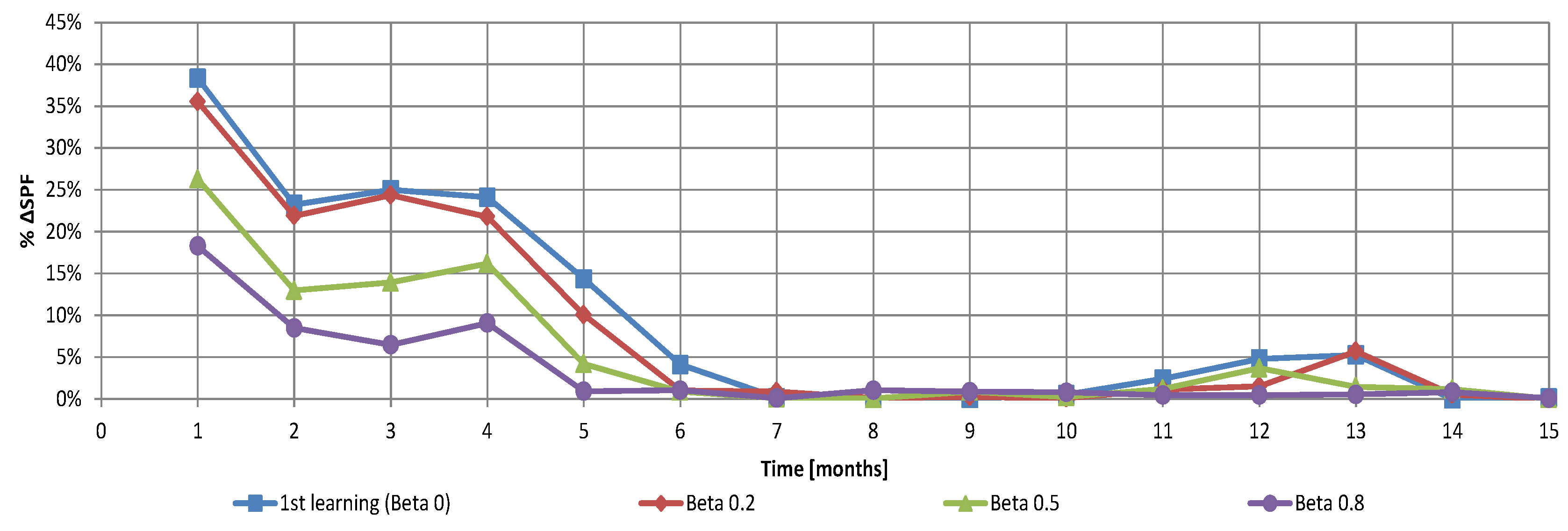
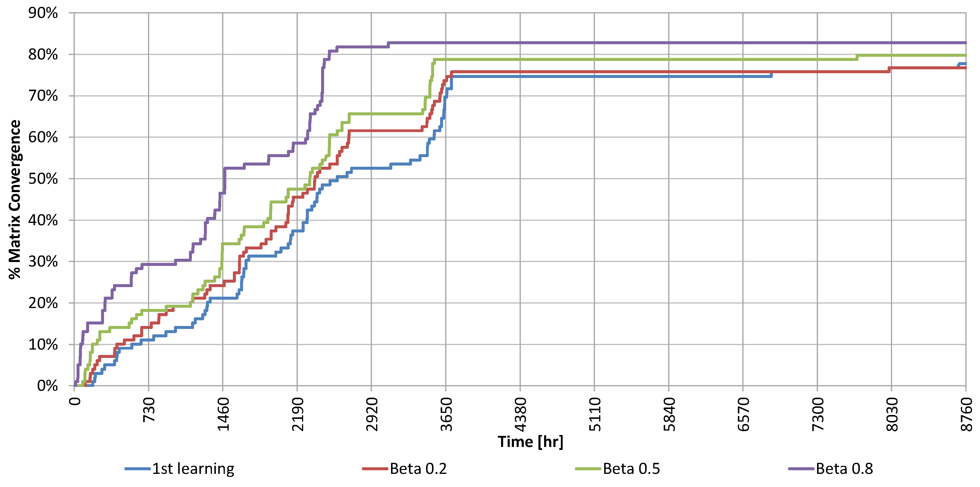
In the last less academic use case, the controller was partially reset after five years of learning using different values of the
parameter without changes in the system. The results are shown in
Figure 15, where the relative errors of SPF
coll (with respect to the convergence values after five years) for four different values of β are plotted, and in
Figure 16, where the exploration factor can be seen.
As expected, the more knowledge was retained the faster the algorithm converged. However, the convergence speed with may seem relatively slow. This is an effect of yearly seasonality. Although the number of explorations per state before reaching convergence was only 2, the exploration was limited because some states were not reachable during that period of the year. This was proven by the fact that the exploration factor tends to form steps where stays constant when all the reachable states have already been fully explored.
4. Conclusions and Future Developments
The results of the controller proposed in this work provide a further confirmation of the benefits of applying a reinforced learning approach to the control of a SDHW system. The main contribution of this paper being that, to the authors’ knowledge, no other study has assessed the performance of a coupled Q-learning-fuzzy control controller on a simple system such as a SDHW. The fact that the underlying system is simple (deterministic) and well known (compared to those investigated in the many works cited in the introductory section generally describing methods to optimize the overall consumptions of a building) has the merit of making immediately clear which component brings what benefit. Moreover, no other study, to the authors’ knowledge, compares the results of such a controller against a simple fuzzy controller alone, and four other simpler control mechanisms (A, B, C and D). The results were not obvious. For example, disregarding certain metrics (circulators on/off cycles), it may turn out that a hysteretic thermostatic control (A), using which there would be no need of installing any micro-processor in a real-life application, is close to providing best system performances.
Regarding the benefits of the proposed controller, experimental results show that it can provide good performance while keeping the number of on/off cycles of the primary circulator low. Looking at this metric, the controller performs only 14% worse than the best reference controller (B), while, at the same time, performing 2.6 time better in terms of SPFcoll. The work shows that the reinforced learning controller can find the best fuzzy controller among those described by a parameter. Looking at the SPFcoll indicator, the new controller shows significantly better performance compared to the best reference cases (between 15% and 115%), while keeping low the number of on/off cycles of the primary pump (1.2 per day down from 30 per day). Regarding the SPFdhw metric, the performance of the self-learning controller was about 11% percent worse than the best reference controller (C). This happened since (a) optimizing the overall performance factor required deciding when to sacrifice solar energy to avoid an unneeded temperature rise, which in turn, required a guess as to when the water would be used in the future; and (b) the creation of a predictor for the DHW load requests was purposely left outside the scope of this work. From this it can be concluded that if the proposed controller is not extended to include a prediction of the load demand, users can be better off relying on a much simpler control strategy. Determining whether this is a fact concerning only the proposed controller or a general fact concerning any so-called smart or advanced SDHW controllers, would require a formal proof or a much broader body of evidence to be gained with further investigations. The literature review indicates that this does not seem to be the case when the energy consumption of an entire building is considered. The last point made by this work is that that the convergence speed of the proposed controller can be increased initialising the algorithm’s internal state with a suitable pre-defined pattern. This is a fundamental property for real-world applications.
Looking for ways to improve the performance of the proposed controller, the most promising option seems to be including a model of the DHW load, which necessarily requires moving from a deterministic approach to a stochastic approach in the problem formulation. Alternative formulations of the reward function, including an extended state, would be required in this case. Another interesting point to be investigated, which seems to be not covered in the literature, is the relation between the γ parameter, the Q-learning cycle time , and the characteristic time constant of the controlled system.


