1. Introduction
The current state of tracking waste containers in municipalities is rigid, inefficient, and hard to oversee [
1]. Following the current shift towards smart cities, there have been attempts to integrate smart technology into urban areas; the most implemented and discussed technology is radio-frequency identification (RFID).
However, this technology needs to be manually employed in containers and the interaction with it must be done locally. This introduces problems of flexibility and cost and a high environmental impact [
2,
3]. To deal with this, we propose a tracking system for waste containers based on computer vision. This solution would remove the constraints and disadvantages of RFID, since it does not require direct interaction with containers or a manual installation of any sort, and, hence, deal with the problems of flexibility and cost and the environmental impact. This is also an opportunity to experiment with computer vision on tasks that involve the use of complex technology. This has been done frequently in industrial settings, but there is a lack of examples on urban scenarios regarding regular activities besides driving or pedestrian detection.
The use of the object recognition approach introduces such problems as an occlusion of containers, perspective shifts, illumination variance, different shapes, scale, and rotation [
4]. The dimension of each problem depends on the scenario and the used object recognition technique. To sum up, the main goal is to be able to successfully identify and classify waste containers in a reliable manner. To achieve this goal, the work presented in this paper makes the following contributions:
Research on approaches to object detection and classification;
The employment of different approaches to object detection, and their implementation in a controlled test scenario; and
An analysis of the results and the possibility of working with the different approaches in the future.
The remainder of this paper is organized as follows.
Section 2 describes the state-of-the-art methods used in this study. These descriptions explore the general concepts and procedure of the methods.
Section 3 details the data and the technology used to serve as a benchmark in the case of replication, how the methods were implemented, and the results obtained from each method. The metrics used to evaluate the results are also pointed out, and the section ends with an analysis of the obtained results.
Section 4 draws conclusions on the work presented in this document and discusses future work.
2. Related Work
The main focus of this study is general object detection and classification, as, with this project, there is a concern with differentiation among types of waste containers [
4].
Currently, there are several approaches to the task of object recognition and classification. There is a requirement to decide amongst the different object recognition techniques: the leading ones in terms of research and results, in their respective fields, are feature-based methods and convolutional neural nets [
5].
The traditional method carries some constraints. The feature detectors and descriptors need to be manually engineered to encode the features. This task is difficult due to the variety of backgrounds, the previously stated transformations, their appearance, and their association with simple and shallow architectures. This approach involves picking features (points) in images that are distinct, repeatable, in great quantities, and accurately localized. Subsequently, these features are described in a way that makes them invariant to several image transformations. Features obtained this way are denoted low-level features, and it is harder to acquire semantic information (information that is useful to recognize objects) from these features [
6]. The majority of waste containers have features that differentiate them. By constructing a database of these features, we can obtain a satisfactory detection rate. The main problem lies in the low flexibility of this approach. The power of this approach comes from its application to limited and specific domains, as seen in [
7,
8].
In the last decade, convolutional neural networks (CNNs) have received more attention and interest from the computer vision community. CNNs constitute a class of models from the broader artificial neural networks field, and they have been shown to produce the best results in terms of efficiency and accuracy [
9]. Their advantages versus traditional methods can be summarized into three main points [
6]: features are represented hierarchically to generate high-level feature representation; the use of deeper architectures increases the expressive capability; and the architecture of CNNs permits the conjunction of related tasks. The architecture itself is also similar to the way an eye works. Similar to an eye, CNNs start by computing low-dimensionality features and end up computing high-dimensionality features that are used for classification. Applying CNNs, specifically to waste containers, provides a major increase in flexibility in the detection and production of results, but only if a proper dataset is obtained and the processing power is reasonable, being the last point the downfall of this approach.
This section is divided into two main topics, each one regarding the previously mentioned methods, and also discusses open research issues.
2.1. Feature-Based Methods
Content-based image retrieval (CBIR) [
10,
11] involves the retrieval of images based on the representation of visual content to identify images that are relevant to the query. The identification of the types of containers is based on what type of image is returned. The CBIR method used in this application is denoted the vector of locally aggregated descriptors (VLAD) [
12,
13].
In order to build a VLAD, descriptors are required, and there is a multitude of them to choose from. In this study, Oriented FAST and Rotated BRIEF (ORB) [
14] was chosen because, unlike other state-of-art descriptors, such as speeded up robust features (SURF) [
15] and scale-invariant feature transform (SIFT) [
16], it is patent-free. Being patent-free is important as this application is intended to have commercial use. Usually, this kind of descriptor is separated into three distinct phases [
4,
16]. In this application, only the first two were necessary.
The first phase is feature detection or extraction. In this phase, an image is searched for locations that are considered likely to match on other images. The second phase is feature description. In this phase, each region around a detected feature is transformed into a numerical descriptor that follows a model to have invariant characteristics.
Each phase introduces important choices. In the feature detection phase, choices need to be made on a feature detection method and the parameters that define a good feature; more precisely, that make an ideal feature. This has been extensively studied in [
17] and more recently in [
18].
In the feature description phase, the problem lies in image transformations. Such transformations can alter a feature’s orientation, illumination, scale, and affine deformation. For these reasons, the chosen descriptor needs to be invariant to the transformations an image can go through [
4]. ORB has some shortcomings; however, it still manages to achieve good results, as demonstrated in [
19].
2.2. Convolutional Neural Networks
The CNNs in the field of computer vision, regarding object detection, can be split in two types: region-proposal-based and regression/classification-based. Regression/classification-based CNNs have better-performing networks with respect to computational cost while maintaining a level of accuracy that is on par with other CNNs. For this reason, this section will be focused on the use of the regression CNN known as you only look once (YOLO) [
20], mainly the last two iterations, which are considered to be state-of-the-art regression-based CNNs [
6].
The CNNs YOLOv2 [
21] and YOLOv3 [
22] were built over YOLO, the first instance of this object detection CNN. This section will be based on the YOLOv2 article [
21], and will delineate its advantages versus other state-of-the-art CNNs with regard to the specific task of object recognition. The YOLOv3 changes are briefly stated at the end of the section.
YOLO performs object detection and classification. In practice, it yields results by surrounding the detected object with a squared box and the predicted class. Regarding complexity, YOLO employs a single neural network to perform predictions of bounding boxes and class probability in one evaluation (hence the name you only look once), which makes it possible to achieve outstanding speed during recognition. Its concepts can be boiled down to three main ideas: (1) the unification of separate common components in object detection into one single neural network; (2) making use of features of an entire image to predict bounding boxes; and (3) the concurrent prediction of all bounding boxes for each class. The inner workings of YOLO will be explained without going deep into the details; this explanation is intended to give the reader a broad idea of its procedure.
YOLO starts out by dividing an input image into a W × W grid cell. Each cell is responsible for detecting an object if the object center falls into it. Then, each cell predicts B bounding boxes and confidence scores for the B predicted boxes. These scores indicate the certainty of an object being present in the box as well as how precise the model believes the box’s prediction is. If there are no objects, the scores should evaluate to zero. Each cell also predicts C conditional probabilities (Class|Object). These probabilities are limited to a cell containing an object.
YOLOv3 is the latest version of this CNN. It is not the primary focus of this study for two reasons: it has a deeper network architecture, and [
22] states that this CNN performs worse when detecting medium-to-large objects. The first reason affects the training and detection phase; a deeper network means that a longer time is necessary for training, and with the current resources the process of training would take a long time to reach a good detection point. The second reason hinders the main goal of this paper, i.e., the detection of large objects.
2.3. Open Research Problems
VLAD is not supposed to perform object detection, at least in the way that is desired. CBIR is a system that retrieves images based on queries and that is not what was intended. VLAD was implemented in part thanks to unfamiliarity with the field of computer vision. However, even if these methods are not the best for the problem at hand, they still produced interesting results.
In contrast to traditional methods, CNNs demonstrate greater potential in the computer vision field. In this study, CNNs were used to substitute an existing technology and yet again prove their flexibility and capacity to adapt to new situations without directly re-engineering their inner workings. The following section delves deeper into the implementations and results for each implementation. It also provides a benchmark scenario for verification of the results.
3. Performance Evaluation
This section starts by stating the hardware and software that were used for each implementation and to obtain the results. Then, we provide a guide for each implementation along with a discussion of the respective results.
3.1. Reference Benchmark Scenario
All of the following implementations were done on a standard ASUS NJ750 with Ubuntu 18.04.1 LTS. The images were all obtained using a Xiaomi Pocophone F1 and resized to 960 × 720 in .jpg format. We used a total of 375 images.
Table 1 demonstrates how they were divided and used. The pictures were taken with different perspectives, illumination settings, and distances relative to containers.
Table 1 demonstrates the picture distribution in terms of illumination settings. The pictures taken were of an emulation of a trash recollection setting, which is detailed as follows. The distance from a container to the camera was never greater than the width of an average road (approximately 10 m). In terms of the camera angle, if the front face of a container is considered to be at 90°, the pictures were taken approximately between 40° and 140°. This study focuses on four different types of containers for which there are some small differences in appearance. A focus on identifying containers with a different appearance is outside the scope of this preliminary study. These pictures also include several examples where there is partial occlusion of the containers to mimic a real scenario. Figures 1, 2, 7, 8, and 9 demonstrate the variety of camera–object distances, camera angles, illuminations, and obstructions.
For both of the implementations, it was necessary to install the OpenCV 3.2.0 library [
23]. For the implementation of VLAD, we used an open-source implementation of VLAD in Python called PyVLAD [
24]. This implementation had some small advantages over the original [
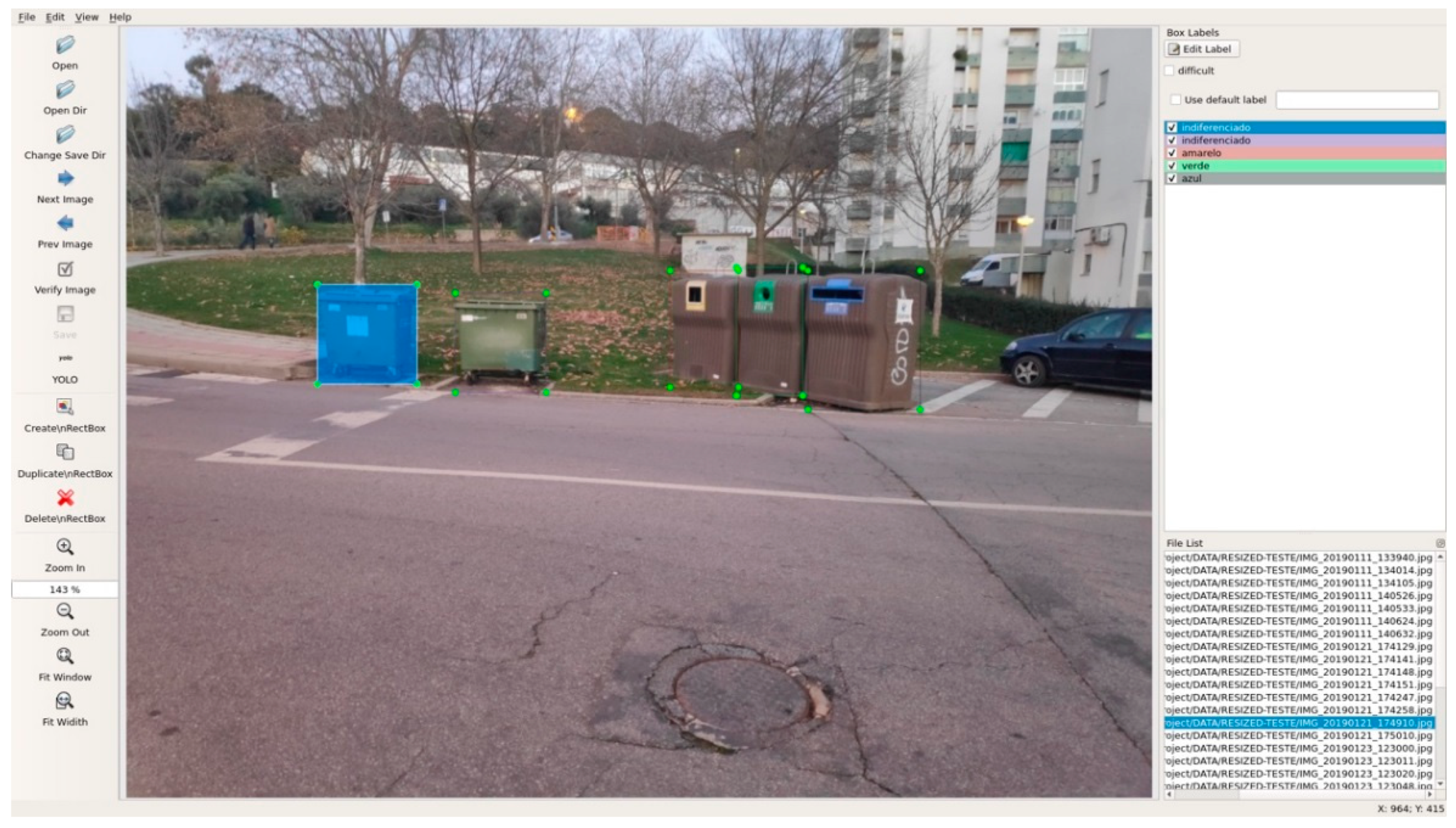
13], such as minor fixes to the code and the addition of multi-threading in the description phase. For YOLOv2 and YOLOv3, the starting point is to prepare the data. This means labeling each container on every picture with the correct bounding box and class.
Figure 1 shows an example of the labeling process. The labeling was done using the labelImg open-source tool [
25].
After the labeling, we used a translation of darknet [
22] to tensorflow, called darkflow [
26], for training and testing the first implementation of YOLOv2. For the second implementation of YOLOv2 and the implementation of YOLOv3, we used a different version of darknet [
27]. It is important to point out that all of the implementations of neural networks had approximately the same amount of training time.
Neural networks almost need to be trained on a graphical processing unit (GPU) due to a GPU’s superiority when performing parallel computation. The use of a GPU requires the installation of CUDA [
28] and cuDNN [
29]; more precisely, CUDA 9.0 and cuDNN 7.1.4. All parameters were left at their defaults or were rearranged to match the computational power available. These changes had no repercussions for the results.
The metrics used to measure the VLAD results were created specifically for this implementation, and the details can be found in the results. For CNNs, the metric used was the mean average precision (mAP) [
30]. For the first implementation of YOLOv2, in order to obtain some of the information about the mAP and the corresponding graphs, the open-source software mAP was used [
31]. For the second implementation of YOLOv2 and the implementation of YOLOv3, the mAP was calculated while the CNN was being trained. This permitted us to plot a graph with the changes in mAP at every fourth iteration. The mean average loss is a metric that is used to identify how well a CNN is being trained and how much longer it needs to be trained. When the average starts to stabilize or reaches a low value, it means that the training process can be stopped.
3.2. VLAD
The implementation of VLAD followed [
12], where it starts with feature detection and description using ORB. Then, each descriptor was associated with the closest cluster of a vocabulary of visual words of size
n. For every cluster, the differences amongst descriptors and cluster centers were accumulated and concatenated in a
n x 32 vector. Then, this vector was square-root normalized and, subsequently,
L2 was normalized. This process was done on every VLAD block to obtain our aggregated local descriptor and attain intra-normalization [
32]. Multi-VLAD was not implemented, since the object retrieval is focused on large-scale objects. Also, vocabulary adaptation was not implemented, as, after obtaining the VLAD descriptors, no data were added.
Since VLAD is not a tool that fits the problem, it was necessary to use it in a different way than its authors intended. First, the images used to create VLAD are single pictures of each container at different settings (illumination, perspective, container). The number of images per class of container is even (56 images, 14 images per class).
The second part was the creation of VLAD using PyVlad. This process is divided into four steps that need to be followed in order: (1) computation of the descriptors using ORB; (2) construction of a visual dictionary using the descriptors calculated during the first step; (3) computation of the VLAD from the visual dictionary and giving each image the appropriate class label; and (4) the creation of an index from the previously computed VLAD descriptors.
With VLAD now computed, it is possible to query the index images containing several containers. This query returns a number of images that are predefined; however, the images themselves are not needed. Only the labels associated with the images are required; as it is with the returned labels that it is possible to obtain results.
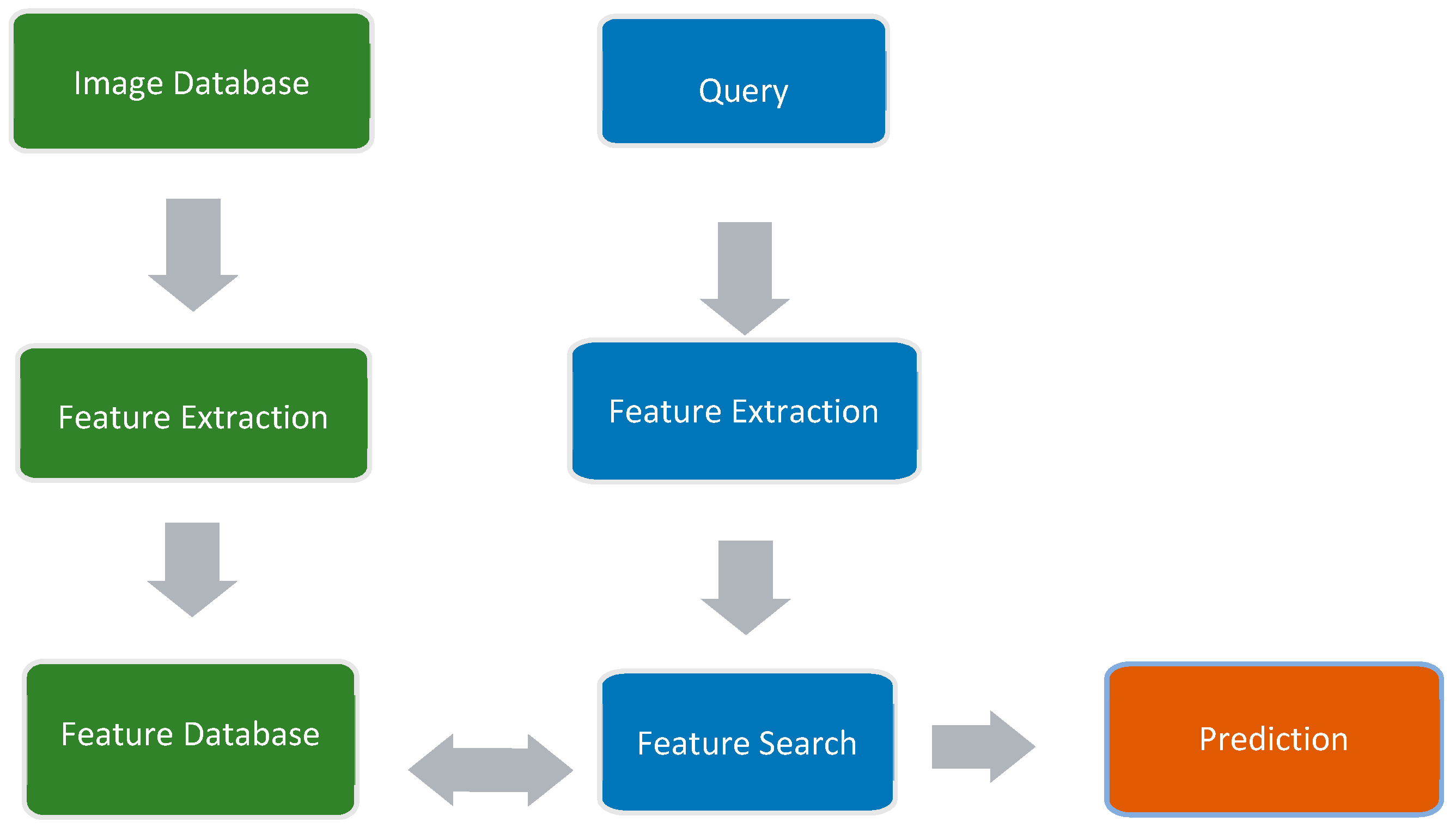
Figure 2 illustrates this process, which has been divided into general topics and separate working areas: green represents the first order of events that is needed to use VLAD; blue represents the process of querying the database containing the extracted information on features; and orange represents the obtained prediction. The method for obtaining results from the predictions is explained in the next paragraph.
The predefined number of labels retrieved from the query was set to 12. After that, a percentage by class is calculated. For example, if the image contains a blue container and the percentage obtained from the labels in the blue class is over 30%, it is counted as a true positive; if it is less than 30%, it is counted as a false positive.
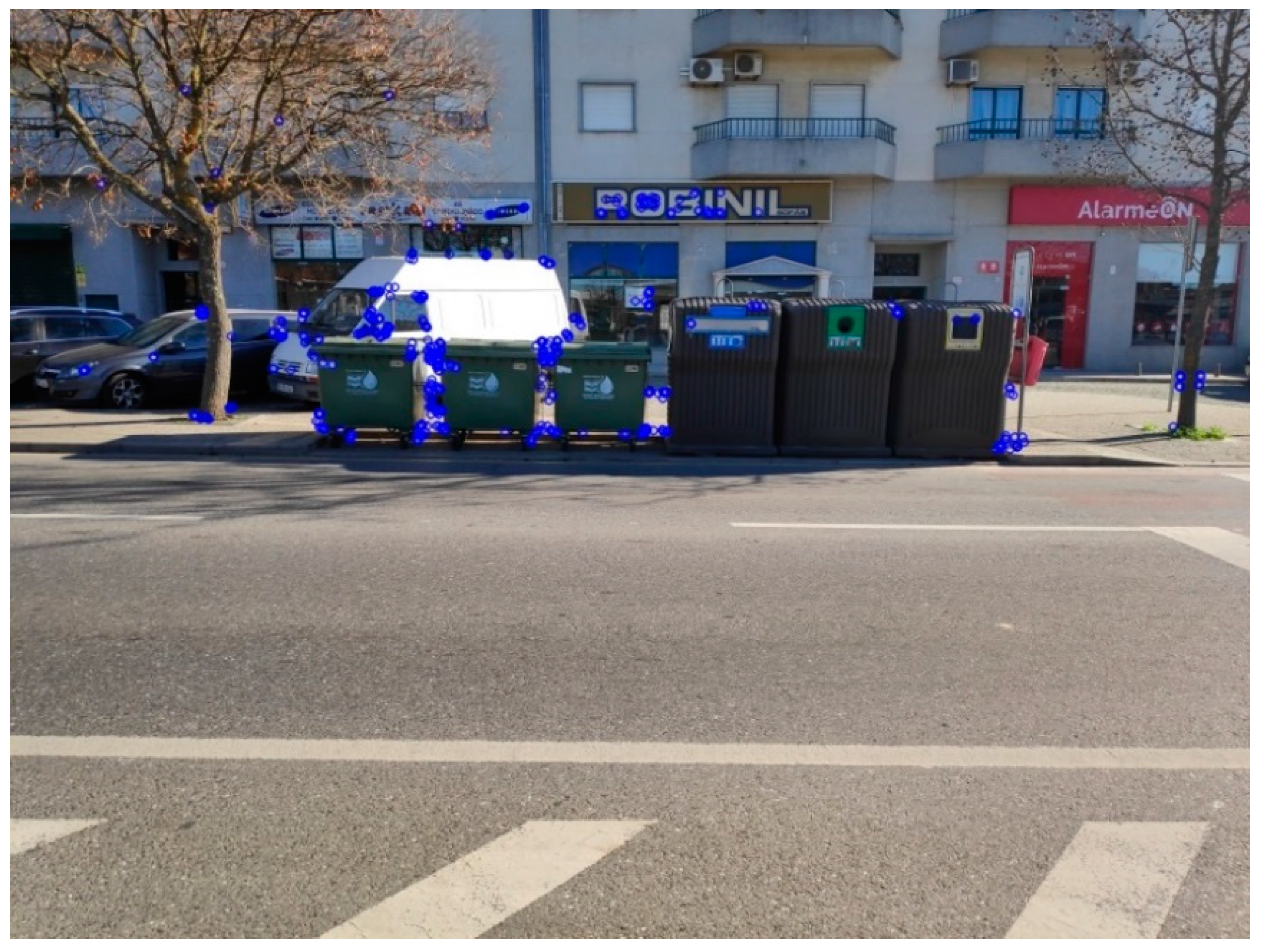
It can be observed from
Table 2 that there is a tendency to always have positive and false results, making the predictions unreliable. The return of labels is limited to the classes, meaning that there will always be at least one true positive, one false positive, and one fail. More interesting is that this is what was observed during the collection of this data. If an image had multiple containers of the same class, the majority of the labels would correspond to that class. The same happens if a container is closer to the camera. This is likely due to the number of descriptors of one class being greater than the rest as seen in
Figure 3, where the blue circles identify the detected ORB features.
3.3. YOLOv2 and YOLOv3
For YOLOv2, the implementation is straightforward. The first step is labelling the images. In this implementation of YOLO, only labelled pictures were used (144 images total). Darkflow has all the tools necessary for training and testing, except the pretrained “.weight” file that needs to be downloaded from the YOLOv2 website [
21]. After that, a python script is created with information about the location of the dataset; the location of the labels; and the used architecture. The python script is executed to start training the CNN. The distribution of the object instances in the training set is shown in
Table 3.
The amount of time that is required to train a neural network depends heavily on the used GPU. On a GTX 850M, it took 9 h to achieve good detection. If trained for too long, the CNN will start to overfit the dataset and its performance during detection will begin to decrease. This is plotted in
Figure 3.
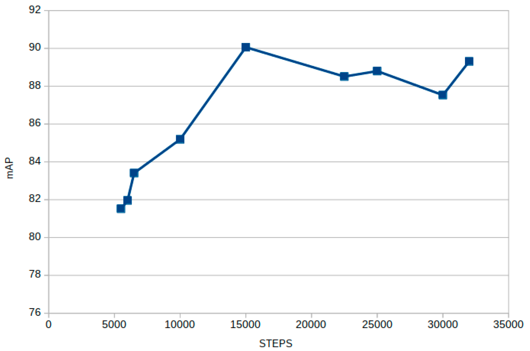
Looking at
Figure 4, the iteration with the highest mAP is at the 15,000-step checkpoint. That is the weight that is going to be used to obtain further results.
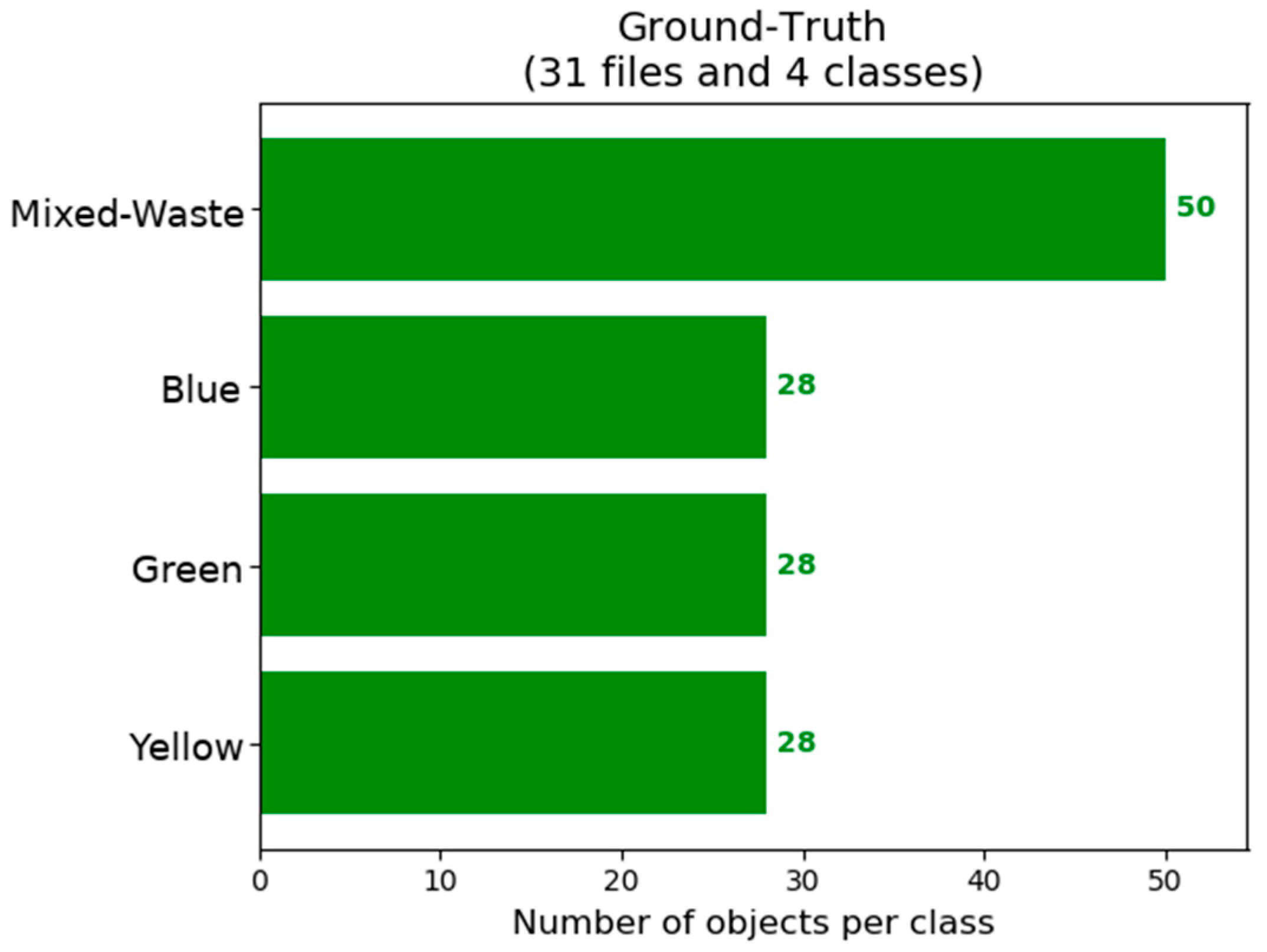
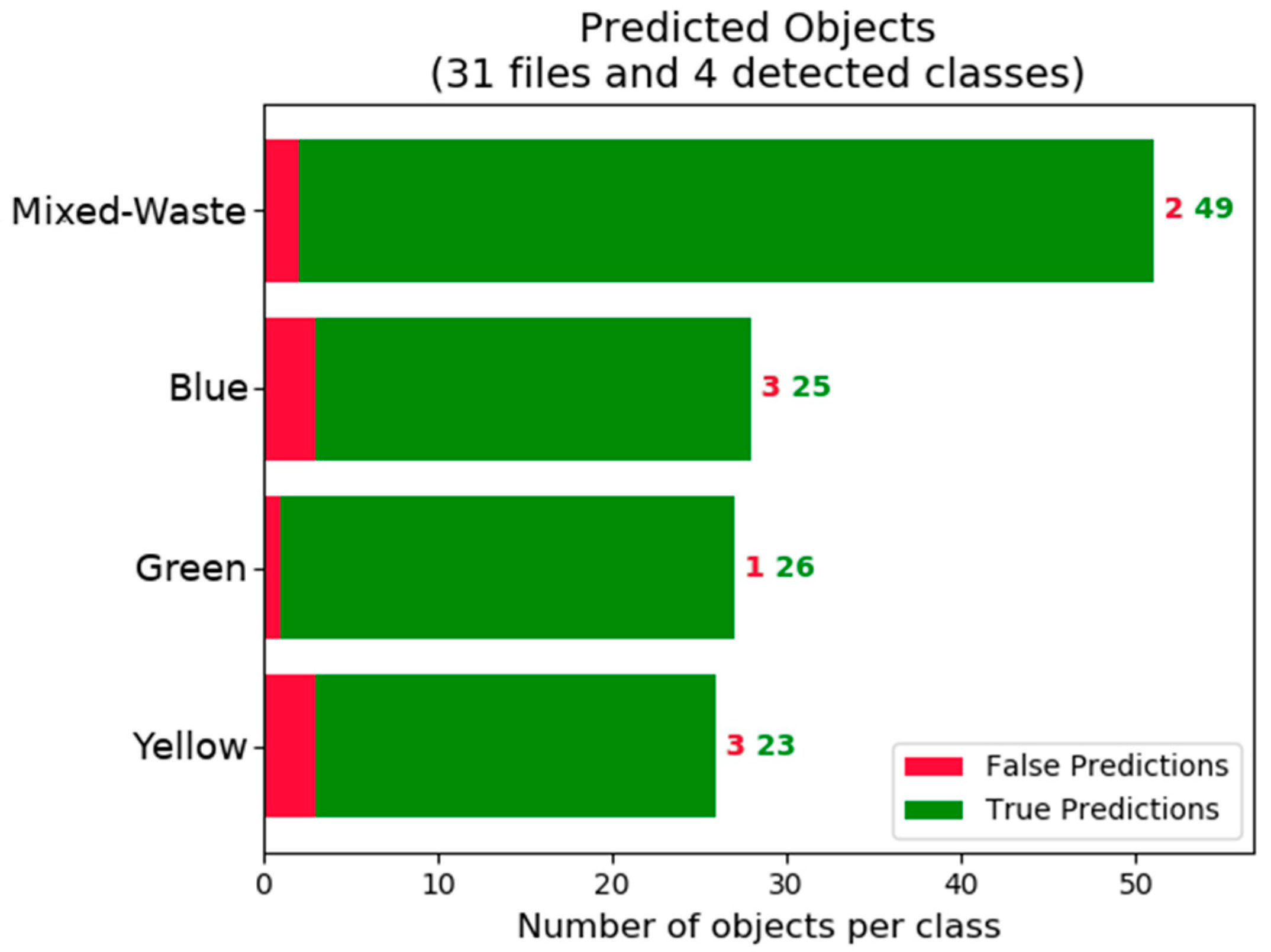
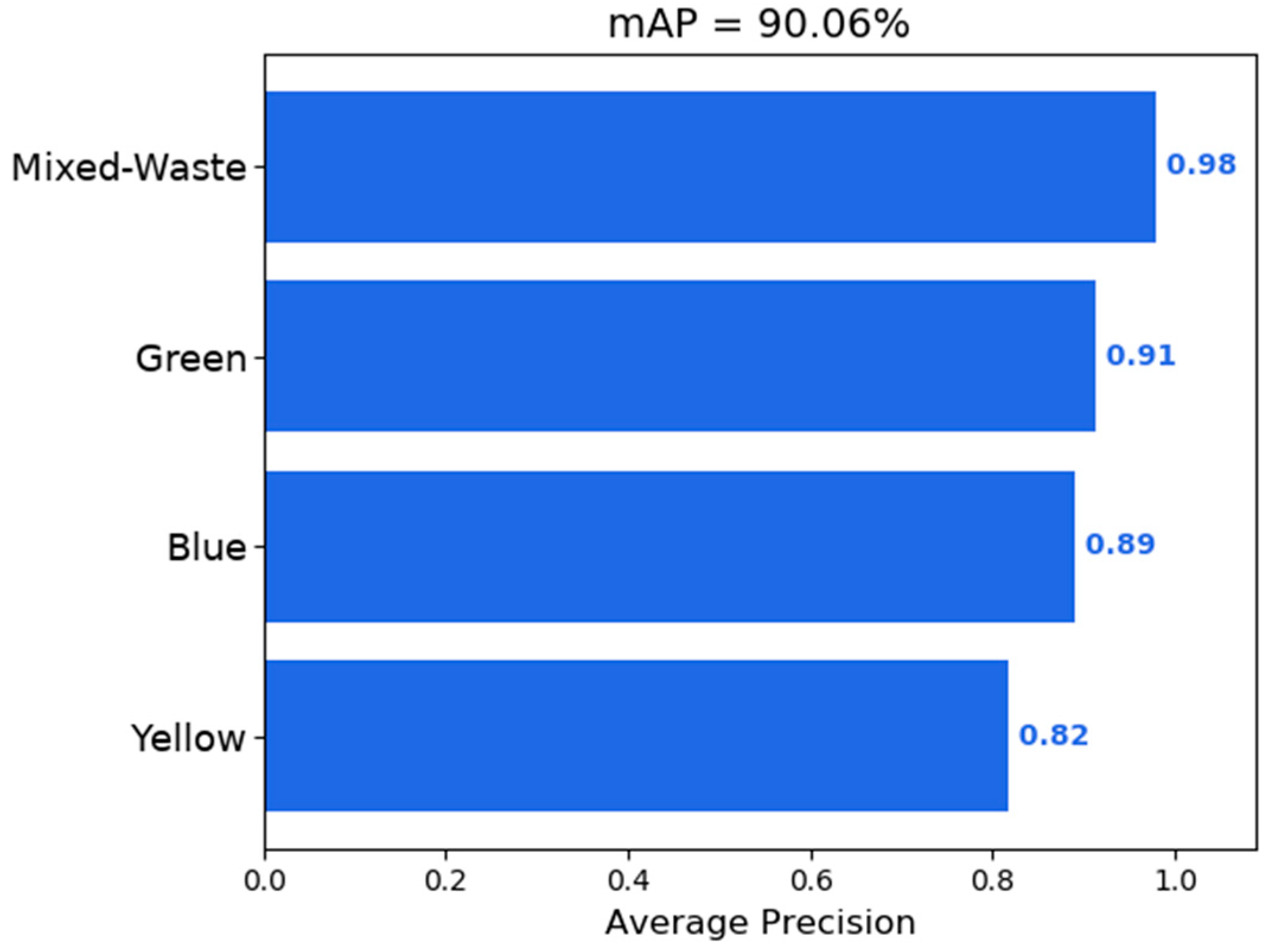
Figure 5 and
Figure 6 show that there is a tendency to obtain better detection of containers in the mixed-waste class. This is attributed to a larger number of instances of this class in the training set as shown by and in part due to the small test dataset that also contains a larger number of mixed-waste containers.
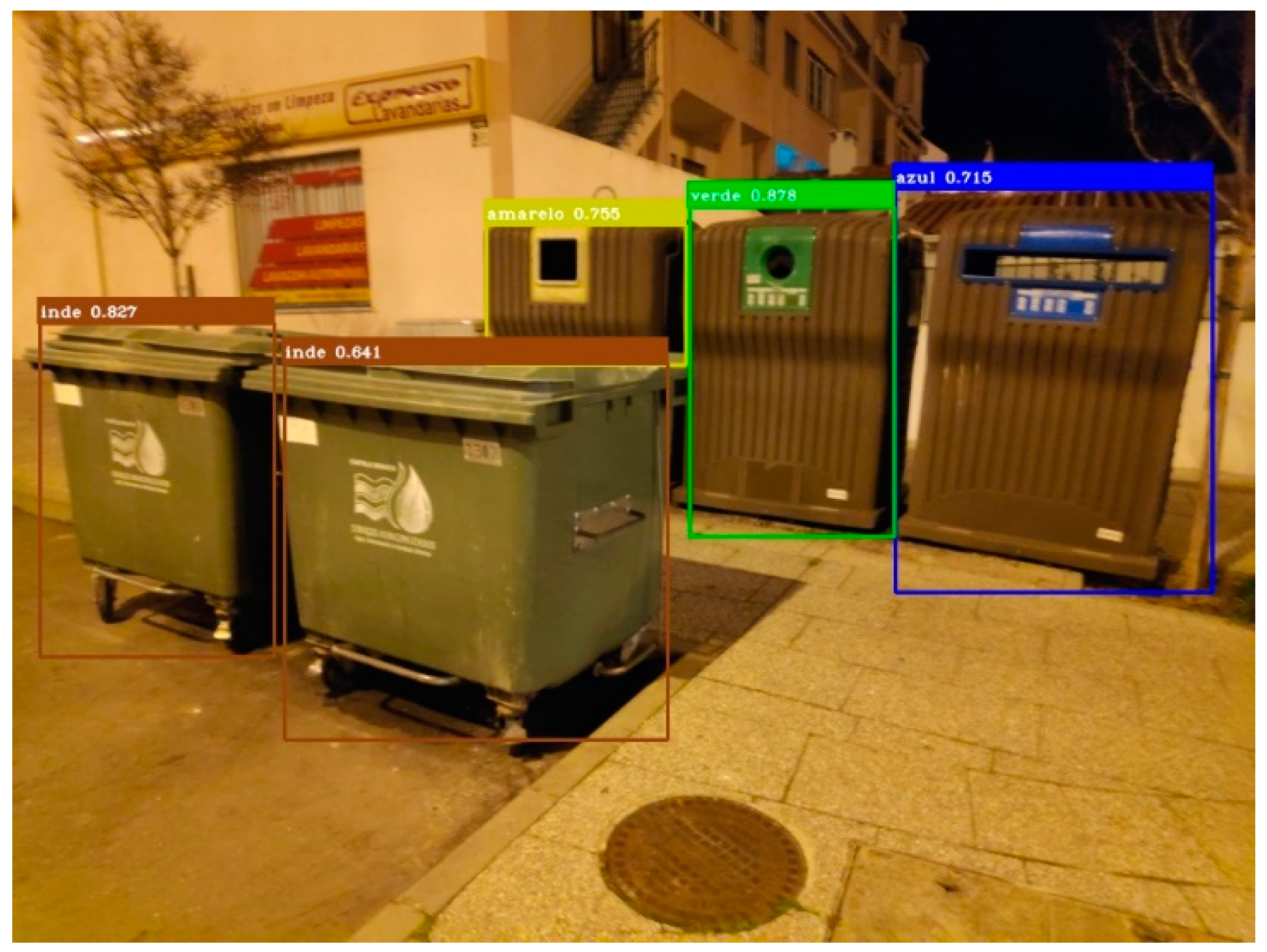
Figure 7 demonstrates an occurrence of a false positive detection.
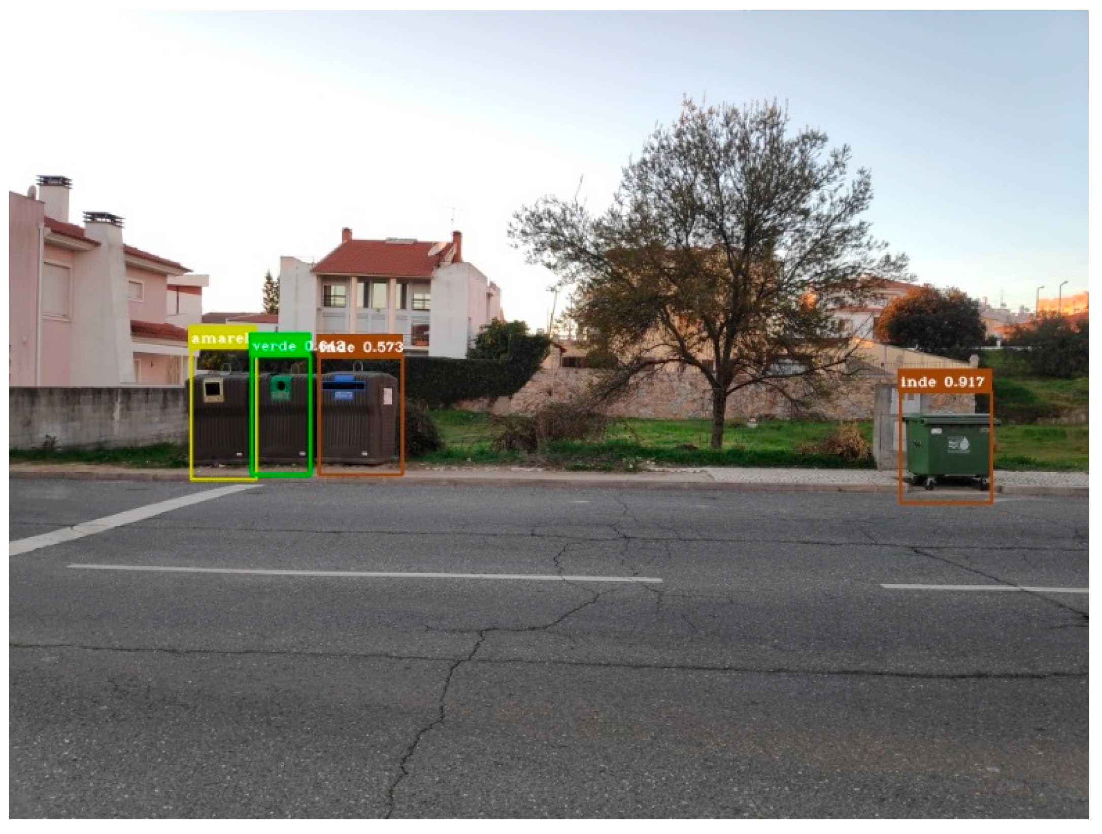
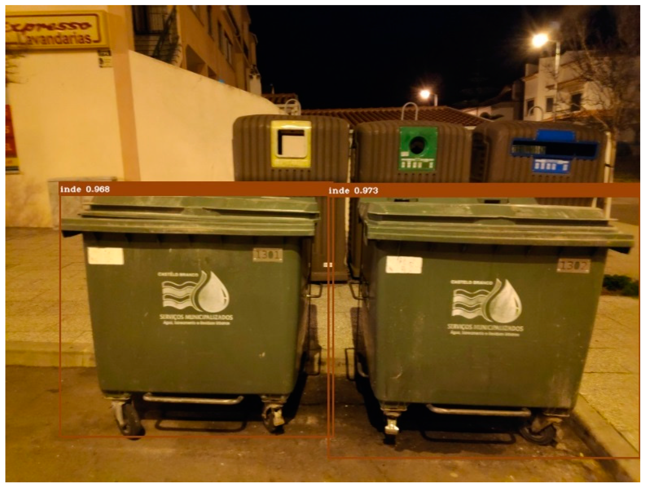
Figure 8 shows that the detection works, even with some occlusion and the same can be seen in the video samples. This is not always the case, as seen in
Figure 9. This robustness to occlusion comes from the training set, where samples with occlusion were used. Video samples that suffer rotation are not able to have reliable detection, since rotation was not present in the training set. The training set should reflect what we can expect from the detection phase.
Unfortunately, the size of the test set is not large, as clearly seen in
Figure 10. The small statistical differences may be due to the size of the test set. Right now, there is no way to be certain without further testing with larger training and testing datasets. The potential of CNNs is undisputed, as these implementations showed a strong capacity for object detection and classification even with limited resources.
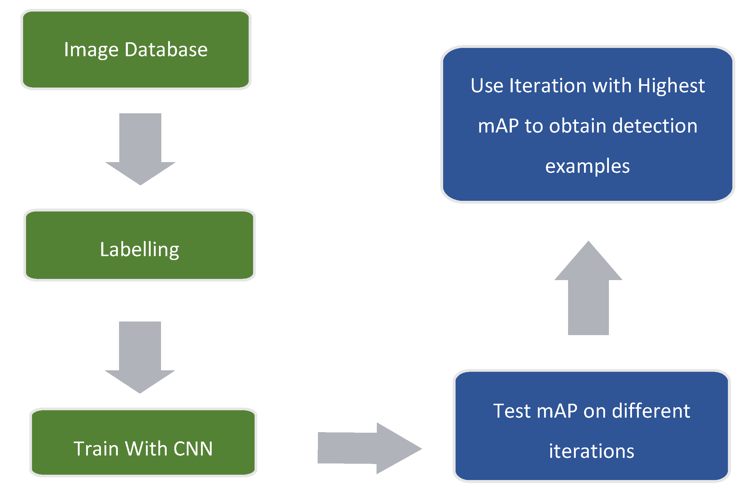
Figure 11 contains a block diagram with the main steps that were followed in order to obtain the presented results and detection examples.
For the second implementation of YOLOv2, we used a total of 288 images. Half of the images comprise of random shots from streets without containers. The addition of these images was done to see whether it improves the mAP during the test.
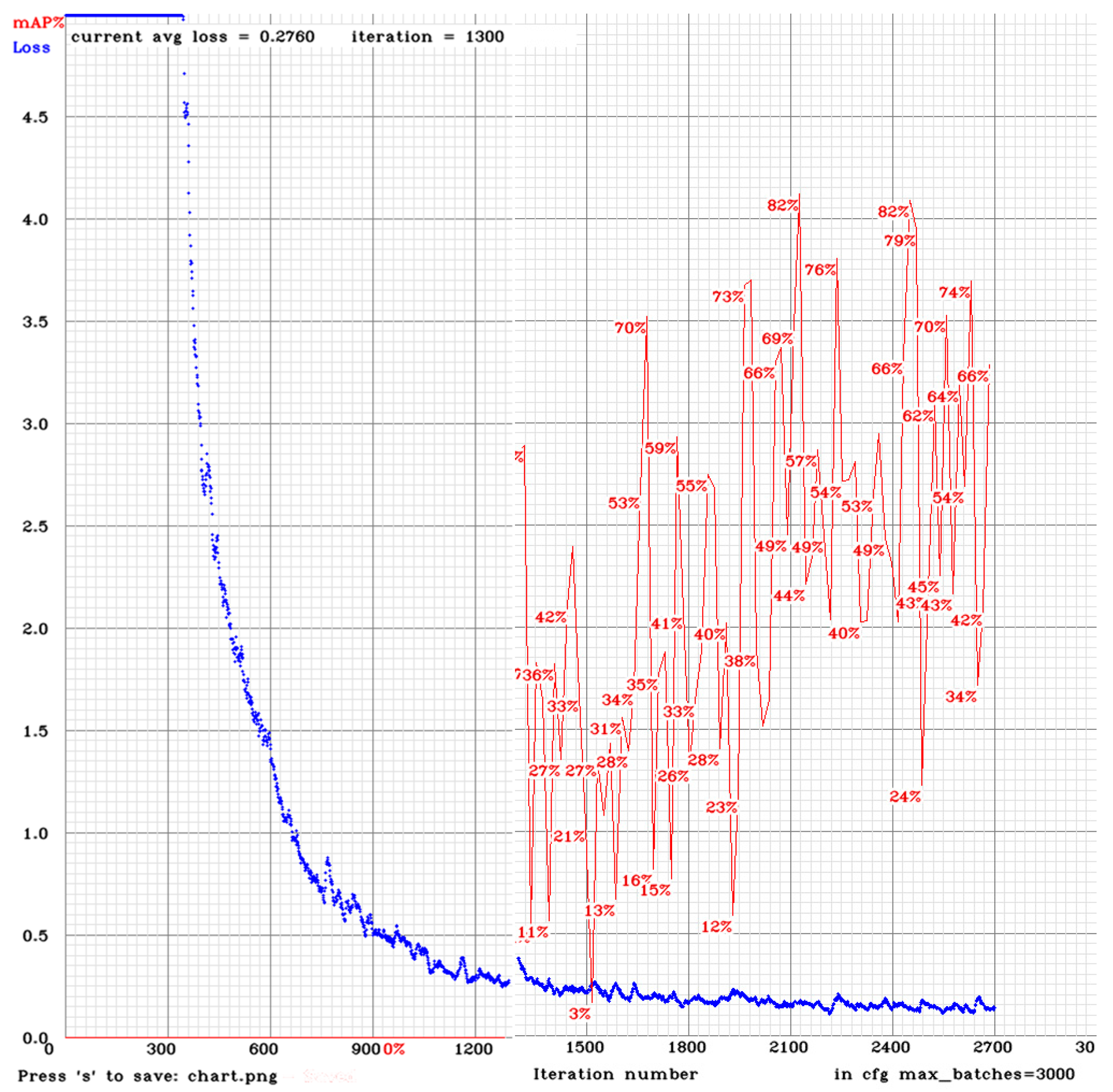
Figure 12 shows how the mAP fluctuates during training. It peaks at 82% around the iterations 2100 and 2460. This mAP value does not reach the 90% mark of the previous implementation. This may be due to the fact that more images were used or that more time was required to reach a higher mAP.
Figure 12 looks a bit off because it is the result of a stitch between two images. This was due to a problem with the first half of the training process, in which the mAP was not being calculated.
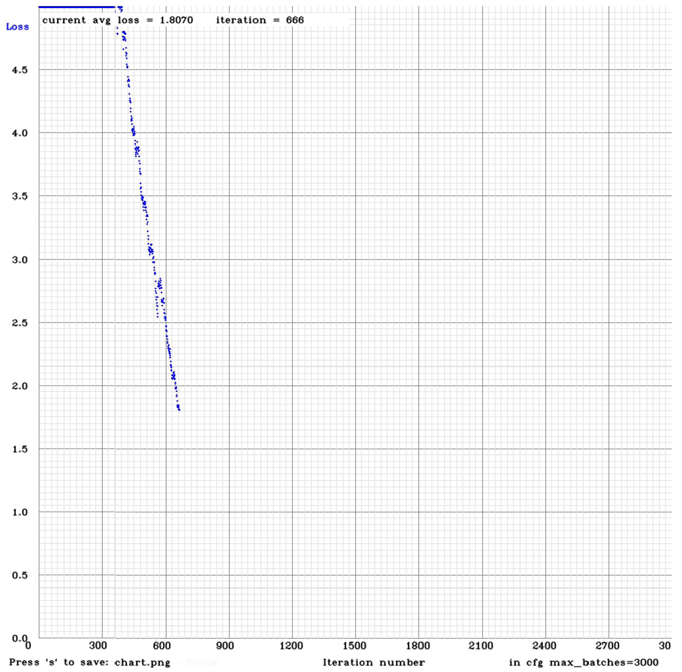
The YOLOv3 architecture is deeper, and, as mentioned earlier, this causes a slower training process. In order to speed up the training process, the calculation of mAP was not applied, and the dataset was comprised of only labelled pictures (144 pictures total). The time that was used for training this implementation was roughly the same as that for the second implementation of YOLOv2. It is important to remember that the second implementation of YOLOv2 had twice as many pictures and was calculating the mAP. Still, after 666 iterations, the average loss was still being reduced and was not stabilizing, as can be seen in
Figure 13.
4. Conclusions
This study focused on the need for a different solution for waste detection and a means to accomplish it using computer vision techniques. This work evaluated different approaches to object detection and classification towards the differentiation of waste container types. Several experiments were performed using feature-based methods and convolutional neural networks.
Regarding VLAD, the implementation will no longer be used as it does not fit the problem of the detection itself. A possible use for this tool would be having a VLAD with images of waste containers at different locations, having those locations be associated with the images, and finding the location of a queried picture that encompasses waste containers. If this kind of scenario is required, then this technique can be revisited. However, in the meantime, there is no use for it considering the results obtained with other implementations.
Concerning CNNs, the detection and classification of the containers peaked at an mAP of 90%. The work with CNNs will be continued, since the achieved results are remarkable given that the results were obtained with constraints on the amount of data, the computational power, and the computation time. These constraints have had a great influence on the acquired results, and this was evident during the implementation of YOLOv3.
The viability of a computer vision approach to replace the current method of detection of waste containers seems promising, although further research and testing needs to be done to make sure the results obtained were not a result of an ad-hoc methodology. As mentioned in the Introduction, if this method produces good and repeatable results, a transfer of target concerning the detection of objects can be initiated.
Future work aims to have a larger dataset with more types of waste containers, as well as a better hardware setup to generate results faster. Since the final goal is to implement this technology in a mobile platform, the created program can complement CNNs. This can involve the creation of a database with geo-locations associated with the detection of waste containers. This information can then be used to confirm a detection or to identify false positives. This process will then generate data that can be used to train CNNs to increase their accuracy.
Author Contributions
All authors contributed to the research, the tests, and the performance evaluations that were presented in this work. All authors contributed to the writing of the paper.
Funding
This work was funded by FCT/MEC through national funds and, when applicable, co-funded by the FEDER–PT2020 partnership agreement under the project UID/EEA/50008/2019.
Acknowledgments
The authors would like to acknowledge the companies EVOX Technologies and InspiringSci, Lda for their interest in and valuable contributions to the successful development of this work.
Conflicts of Interest
The authors declare no conflict of interest.
References
- Zanella, A.; Bui, N.; Castellani, A.; Vangelista, L.; Zorzi, M. Internet of things for smart cities. IEEE Internet Things J. 2014, 1, 22–32. [Google Scholar] [CrossRef]
- Abdoli, S. RFID application in municipal solid waste management system. IJER 2009, 3, 447–454. [Google Scholar] [CrossRef]
- Gnoni, M.G.; Lettera, G.; Rollo, A. A feasibility study of a RFID traceability system in municipal solid waste management. Int. J. Inf. Technol. Manag. 2013, 12, 27. [Google Scholar] [CrossRef]
- Szeliski, R. Computer Vision: Algorithms and Applications; Springer Science & Business Media: Berlin, Germany, 2010. [Google Scholar]
- Achatz, S. State of the Art of Object Recognition Techniques. Sci. Semin. Neurocientific Syst. Theory 2016. [Google Scholar]
- Zhao, Z.-Q.; Zheng, P.; Xu, S.; Wu, X. Object detection with deep learning: A review. arXiv, 2018; arXiv:1807.05511. [Google Scholar]
- Hu, F.; Zhu, Z.; Zhang, J. Mobile panoramic vision for assisting the blind via indexing and localization. In European Conference on Computer Vision; Springer: Berlin, Germany, 2014; pp. 600–614. [Google Scholar]
- Niu, J.; Lu, J.; Xu, M.; Lv, P.; Zhao, X. Robust lane detection using two-stage feature extraction with curve fitting. Pattern Recognit. 2016, 59, 225–233. [Google Scholar] [CrossRef]
- Zheng, L.; Yang, Y.; Tian, Q. SIFT meets CNN: A decade survey of instance retrieval. IEEE Trans. Pattern Anal. Mach. Intell. 2018, 40, 1224–1244. [Google Scholar] [CrossRef] [PubMed]
- Zhou, W.; Li, H.; Tian, Q. Recent Advance in Content-based Image Retrieval: A Literature Survey. arXiv, 2017; arXiv:1706.06064. [Google Scholar]
- Kumar, K.K. CBIR: Content Based Image Retrieval. In Proceedings of the National Conference on Recent Trends in Information/Network Security, Chennai, India, 12–13 August 2010; Volume 23, p. 24. [Google Scholar]
- Jégou, H.; Douze, M.; Schmid, C.; Pérez, P. Aggregating local descriptors into a compact image representation. In Proceedings of the IEEE Conference on Computer Vision and Pattern Recognition (CVPR), San Francisco, CA, USA, 13–18 June 2010; pp. 3304–3311. [Google Scholar]
- Diaz, J.G. VLAD. GitHub Repository. 2017. Available online: https://github.com/jorjasso/VLAD (accessed on 14 February 2019).
- Rublee, E.; Rabaud, V.; Konolige, K.; Bradski, G. ORB: An efficient alternative to SIFT or SURF. In Proceedings of the 2011 IEEE International Conference on Computer Vision (ICCV), Barcelona, Spain, 6–13 November 2011; pp. 2564–2571. [Google Scholar]
- Bay, H.; Tuytelaars, T.; van Gool, L. Surf: Speeded up robust features. In Proceedings of the European Conference on Computer Vision, Graz, Austria, 7–13 May 2006; pp. 404–417. [Google Scholar]
- Lowe, D.G. Distinctive image features from scale-invariant keypoints. Int. J. Comput. Vis. 2004, 60, 91–110. [Google Scholar] [CrossRef]
- Tuytelaars, T.; Mikolajczyk, K. Local invariant feature detectors: A survey. Found. Trends® Comput. Graph. Vis. 2008, 3, 177–280. [Google Scholar] [CrossRef]
- Salahat, E.; Qasaimeh, M. Recent advances in features extraction and description algorithms: A comprehensive survey. In Proceedings of the 2017 IEEE International Conference on Industrial Technology (ICIT), Toronto, ON, Canada, 22–25 March 2017; pp. 1059–1063. [Google Scholar]
- Miksik, O.; Mikolajczyk, K. Evaluation of local detectors and descriptors for fast feature matching. In Proceedings of the 21st International Conference on Pattern Recognition (ICPR), Tsukuba, Japan, 11–15 November 2012; pp. 2681–2684. [Google Scholar]
- Redmon, J.; Divvala, S.; Girshick, R.; Farhadi, A. You only look once: Unified, real-time object detection. In Proceedings of the IEEE Conference on Computer Vision and Pattern Recognition, Las Vegas, NV, USA, 27–30 June 2016; pp. 779–788. [Google Scholar]
- Redmon, J.; Farhadi, A. YOLO9000: Better, faster, stronger. arXiv preprint. ArXiv161208242. Available online: https://arxiv.org/abs/1612.08242 (accessed on 25 December 2016).
- Redmon, J.; Farhadi, A. Yolov3: An incremental improvement. arXiv, 2018; arXiv:1804.02767. [Google Scholar]
- Bradski, G. The OpenCV Library. Dr. Dobb’s J. Softw. Tools 2000, 25, 120–125. [Google Scholar]
- Bober-Irizar, M. PyVLAD. GitHub Repository. 2017. Available online: https://github.com/mxbi/PyVLAD (accessed on 14 February 2019).
- Lin, T. labelImg. GitHub Repository. 2019. Available online: https://github.com/tzutalin/labelImg (accessed on 14 February 2019).
- Trieu, T.H. Darkflow. GitHub Repository. Available online: https://github.com/thtrieu/darkflow (accessed on 14 February 2019).
- Bezlepkin, A. Darknet. GitHub Repository. 2019. Available online: https://github.com/AlexeyAB/darknet (accessed on 14 February 2019).
- NVIDIA Corporation. NVIDIA CUDA Compute Unified Device Architecture Programming Guide; NVIDIA Corporation: Santa Clara, CA, USA, 2007. [Google Scholar]
- Chetlur, S.; Woolley, C.; Vandermersch, P.; Cohen, J.; Tran, J.; Catanzaro, B.; Shelhamer, E. Cudnn: Efficient primitives for deep learning. arXiv, 2014; arXiv:1410.0759. [Google Scholar]
- Everingham, M.; van Gool, L.; Williams, C.K.I.; Winn, J.; Zisserman, A. The pascal visual object classes (voc) challenge. Int. J. Comput. Vis. 2010, 88, 303–338. [Google Scholar] [CrossRef]
- Cartucho, J. map. GitHub Repository. 2019. Available online: https://github.com/Cartucho/mAP (accessed on 14 February 2019).
- Arandjelovic, R.; Zisserman, A. All about VLAD. In Proceedings of the IEEE Conference on Computer Vision and Pattern Recognition, Portland, OR, USA, 23–28 June 2013; pp. 1578–1585. [Google Scholar]
© 2019 by the authors. Licensee MDPI, Basel, Switzerland. This article is an open access article distributed under the terms and conditions of the Creative Commons Attribution (CC BY) license (http://creativecommons.org/licenses/by/4.0/).


 ,
, 


