Article

Hidden Sea Level Effect on Mediterranean Outflow Proxies

by
Javier P. Tarruella
1,2,* and
Francisco J. Sierro
3,4
1
Área de Paleontología, Departamento de Geología, Universidad de Salamanca, 37008 Salamanca, Spain
2
Área de Estratigrafía, Departamento de Ciencias de la Tierra y del Medio Ambiente, Universidad de Alicante, 03080 Alicante, Spain
3
School of Geographical Sciences, University of Bristol, University Road, Bristol BS8 1SS, UK
4
Departamento de Geología (Grupo GEAPAGE), Universidad de Salamanca, 37008 Salamanca, Spain
*
Author to whom correspondence should be addressed.
Quaternary 2026, 9(5), 65; https://doi.org/10.3390/quat9050065 (registering DOI)
Submission received: 20 August 2026 / Revised: 13 September 2026 / Accepted: 16 September 2026 / Published: 18 September 2026

Abstract

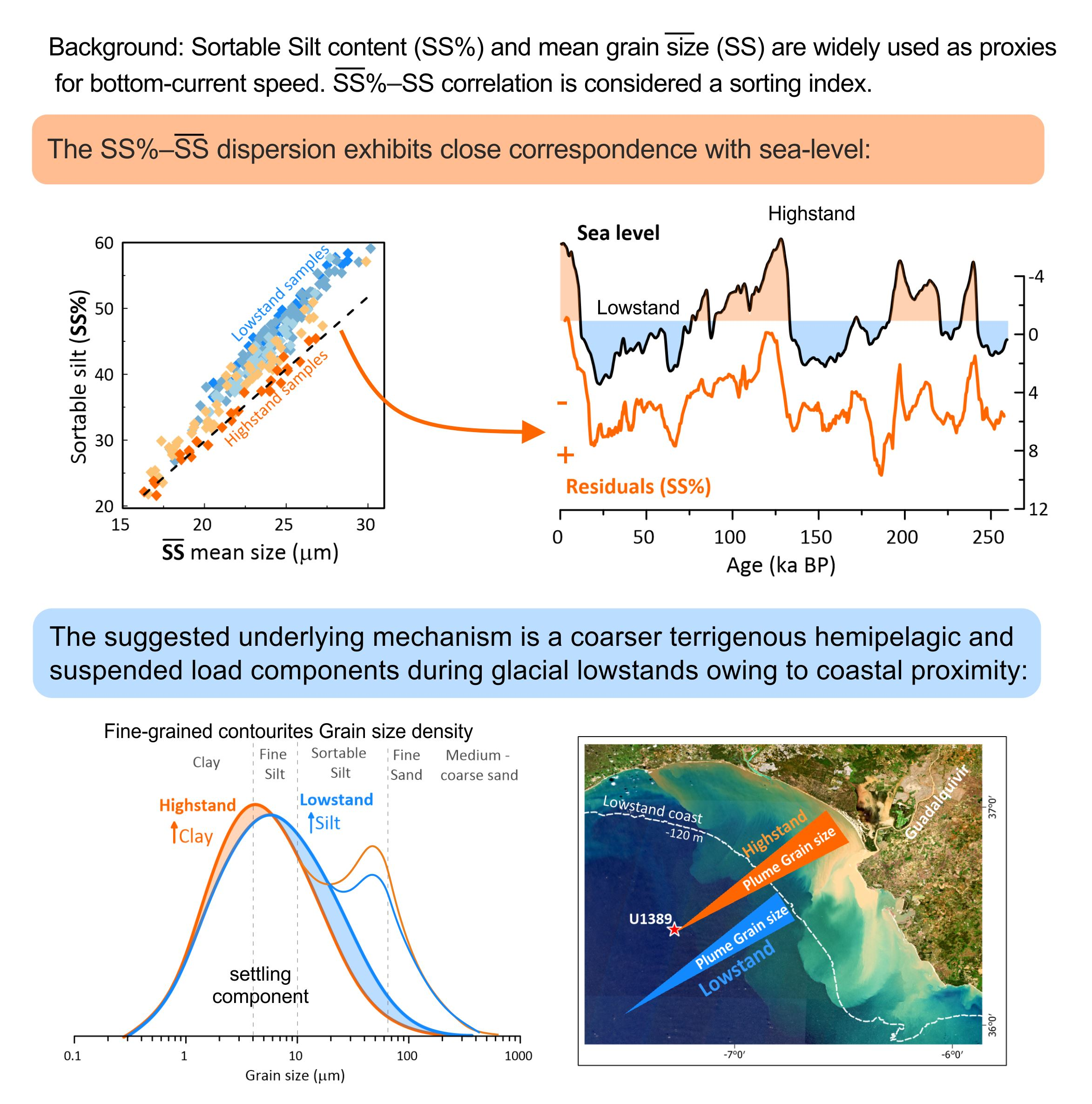
Contourite activity in the Gulf of Cadiz (GoC) is dominated by the precession-driven, ~20 ka cyclicity of the Mediterranean circulation and Mediterranean Outflow Water (MOW). Grain size distributions in contourites are strongly influenced by bottom current speed and are therefore widely used in the GoC to trace past MOW strength changes. However, the influence of sea level changes, driven by the expansion and retreat of ice sheets following the “100 ka world”, is superimposed to some extent through variations in terrigenous sediment supply. Despite the numerous high-resolution proxy records of MOW strength, the influence of glacial–interglacial relative sea level (RSL) changes on these records remains unclear. By analyzing the correlation between sortable silt grain size parameters at IODP U1389, we isolated the grain size variability that is not controlled by bottom current (MOW) sorting. This residual grain size variability closely follows the RSL curves and accounts for the higher sortable silt content observed during RSL lowstands. We suggest that the RSL-induced shoreline proximity contributes to a coarser terrigenous hemipelagic/suspended load component in contourites, increasing silt content. Furthermore, we present novel outflow proxy records based on the specific mineral components by using mica (allogenic) and pyrite (authigenic) counts.

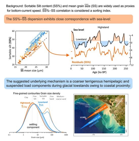
Graphical Abstract

1. Introduction

Mediterranean Outflow Water (MOW) constitutes a contouritic current that has generated the most extensive contourite depositional system in the world [1]. The flow of MOW along the Gulf of Cadiz (GoC), on the northeastern Atlantic margin (Figure 1), has generally been reconstructed via grain size analyses of sediments deposited under the influence of this contouritic current [2,3,4,5]. These sediments originate from markedly different sources: the biogenic fraction is mainly composed of planktonic foraminifera and coccoliths; the detrital fraction mainly derives from terrestrial material supplied by rivers to the continental shelf and upper slope [6,7], which is subsequently captured and transported alongslope by MOW [4,8].
Under the influence of MOW on the middle slope of the GoC, sediment grain size distribution is strongly controlled by bottom current speed [5,8]. Since the middle Pleistocene, sedimentation has been governed by two main processes: the settling of fine-grained sediments from suspension (dominant process during weak MOW periods) and the deposition of detrital grains mainly transported by saltation as bedload (dominant process during strong MOW periods) [8,9]. Thus, contouritic sediments have a mixed origin, as reflected by their usually bimodal grain size distributions [8]. Under weakened MOW, the fine-grained hemipelagic background settling constitutes a significant fraction of the sediment [8]. This hemipelagic component progressively decreases under increasing bottom current speed, promoting the resuspension and winnowing of the fine-grained material [10,11]. Both via grain sorting and via winnowing the fine-grained fraction, the MOW flow speed exerts the major control on grain size distributions [8].
During glacial periods, terrigenous sediment supply generally increases as sea level fall causes the shoreline and river mouths to migrate closer to the shelf edge [12] (Figure 1). At IODP Site U1389, several proxies reflect this glacial (RSL lowstand) increase in sediment supply, including overall higher sedimentation rates, increased natural gamma radiation, and changes in clay mineral composition [6,10,11]. While MOW flow strength is mainly controlled by changes in Mediterranean termohaline circulation, driven by precession-related ~20 ka climate cycles, terrigenous clay–silt supply is mainly controlled by sea level [6,12], governed by the 100 ka periodicity of glacial–interglacial cycles since the Middle Pleistocene Transition [13,14], and climate [15]. However, the strong influence of MOW strength on sediment grain size distributions is concomitantly superimposed to the clay–silt supply signal, concealing the latter variable [10]. Outside the influence of MOW, sedimentation on the adjacent continental shelf is indeed mainly controlled by glacial–interglacial sea level changes, which enhance terrigenous supply and generate regressive sequences during lowstands [12]. Sea level generally controls the partition of riverine terrigenous material among the shelf, slope, and abyssal plain, increasing sedimentation rates in the latter environments during lowstands [2,16]. Along the middle slope, at intermediate depths, the reduced activity of the upper MOW branch during glacial periods may also contribute to increased sedimentation rates through reduced winnowing [4,17].
MOW flow speed proxy records at IODP Site U1389 have been obtained from a broad range of grain size and sediment composition analyses. Regarding grain size, the proportion of very fine sand [2,18,19], as well as that of sortable silt ( g r a i n   s i z e   10 63   μ m ) [5,20], is considered representative of the detrital fraction and thus proportional to the MOW flow speed. Conversely, >150 µm is mainly composed of foraminifera and other bioclasts [7], whereas fine silt and clay predominantly comprise hemipelagic terrigenous material and nanoplankton [11]. The mean size of sortable silt ( S S ¯ ) is considered proportional to the bottom current speed [21], and it has been used to quantify MOW flow speed in absolute terms [4,5]. The S S ¯ –SS% correlation is considered a current sorting index for paleoflow, and timeseries running correlation is used to validate grain size data as records for flow history [22]. Regarding composition, major element ratios derived from XRF analyses, such as Zr/Al [23], Zr/Rb [4], and Zr/Ti ratios [11], have also been used to reconstruct MOW strength. In these ratios, zirconium (Zr) represents the coarser terrigenous fraction (heavy detrital minerals); K, Al, Rb, K, and eventually Ti are considered proxies for the finer terrigenous fraction (fine silt–clay) [4,8,24], which arrives via river sediment plumes, aeolian dust, and nepheloid layers and as suspended load [7,25,26]. Therefore, these ratios are also affected by changes in terrigenous supply in addition to variations in MOW strength. Several studies used these and other bottom current proxies to identify astronomical cycles and to tune age models through correlation between MOW contourite activity and astronomical curves [5,15]. One of the most significant features is the occurrence of dominant hemipelagic sedimentation, indicative of very weak bottom current activity, during periods of Eastern Mediterranean stagnation and sapropel deposition, around precession minima [15,19,23].
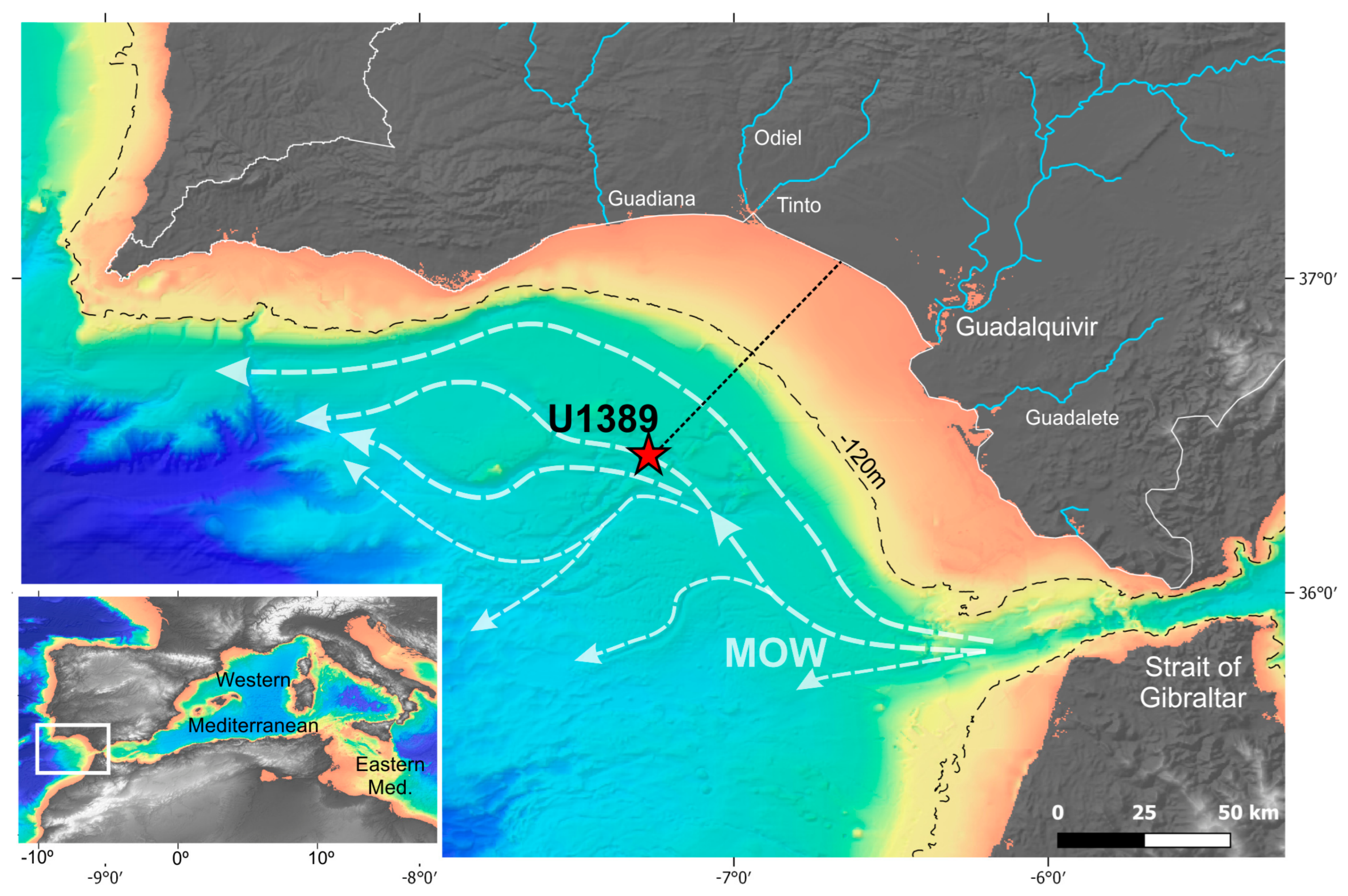
The IODP Site U1389 (36°25.515′ N, 7°16.683′ W, 640 mbsl), located on the middle slope in the central GoC (Figure 1), has become a reference site for reconstructing MOW strength over the last several glacial–interglacial cycles. This site was drilled into a sheeted-drift deposit, whose high sedimentation rates (up to 100 cm×ka−1) and stratigraphic continuity enable high-resolution palaeoceanographic reconstructions [27,28]. The sedimentary record at U1389 is characterized by the strong precession-related cyclicity described above (~20 ka period), increasing the hemipelagic content (indicating reduced MOW strength) during precession minima, coeval with Mediterranean sapropel deposition [2,23,29]. This pronounced precession-driven cyclicity contrasts with the global climate variability since the Middle Pleistocene Transition, characterized by the global expansion and retreat of ice sheets, dominated by the eccentricity-driven glacial–interglacial cycles [13,14]. During glacial periods, millennial-scale variability is superimposed on orbital variability, in which Greenland stadials (GSs) correspond to relatively high MOW speed and Greenland interstadials (GIs) to relatively low MOW speed [18,19,30].
Figure 1. The oceanographic setting of IODP Site U1389 (red star) in the middle slope of the Gulf of Cadiz, ~150 km away from the Atlantic–Mediterranean gateway. White arrows: The Mediterranean outflow pathway. The −120 m isobath is represented to illustrate the potential glacial–interglacial shoreline displacement. Note that during glacial maxima, distance to the coast can reach half of that of today. The main rivers of the GoC are represented in blue. Bathymetry data from [31].
Quaternary 09 00065 g001
Although the proportion of the detrital fraction and its mean grain size are commonly assumed to be indicators of paleocurrent activity, factors other than bottom current speed may also influence the final detrital content of the sediment [2,32]. In this study, we analyzed the relationship between S S ¯ and SS% in response to glacial–interglacial relative sea level changes and their influence on terrigenous sediment supply to the middle slope. By this approach, we aim to successfully isolate the RSL influence on contouritic sediments. Furthermore, we investigated the nature of the particles composing the sandy fraction of contourite deposits at Site U1389 to explore new MOW strength proxies based on specific mineral components.

2. Materials and Methods

2.1. IODP Site U1389 Core Samples

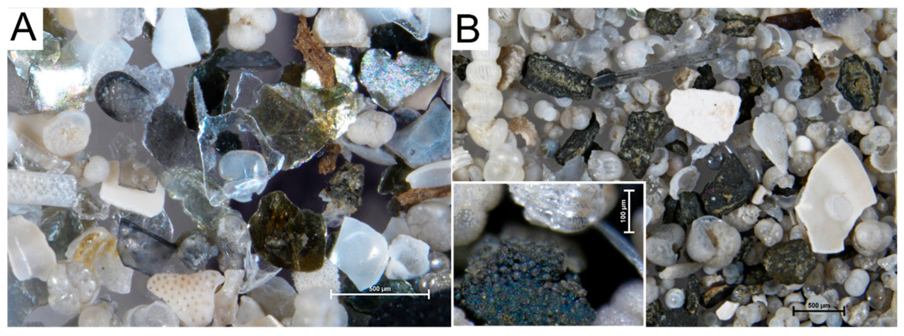
For sediment composition visual analysis, 296 samples from the top 95 mcd (meters composite depth) were analyzed (mean sampling rate = 17 cm). Approximately 12 cm3 of sediment was collected from each sample, freeze-dried, and weighted. The samples were then disaggregated in water and wet-sieved at 62 µm to remove the clay- and silt-sized fractions. The >63 µm residue was dried and sieved again at 150 µm. Sandy fractions and bulk sediment weights were published by [2]. The >150 µm fraction was divided into halves using a microsplitter until a representative subsample was obtained (n > 300 particles; [33]) and subsequently examined under a binocular microscope. All particles in the >150 µm fraction were identified and counted (average n = 1463 particles/sample; total particles = 433,453). Particular attention was paid to the main authigenic and allogenic minerals present in this fraction, which are pyrite and micas, respectively (Figure 2). Particle contents were expressed as density (n particles > 150 µm/g of bulk sediment) and as percentages (n particles > 150 µm/total particles > 150 µm). To eliminate the effect of sediment dilution, particle content was also expressed as fluxes, obtained as follows:
F l u x = n   c o u n t s × 2 n   s p l i t s b u l k   w e i g h t   g × 1.9   g c m 3 × c m k a = n   p a r t i c l e s c m 2 × k a

2.2. Age Model

The age model was adopted from [2] for the last 265 ka, which encompasses the main period studied. This age model was established by using radiocarbon dating and by tuning the high-resolution record of the δ18O of planktic foraminifer Globigerina bulloides (Figure 3G) to the Greenland δ18O synthetic records [34], according to the INTIMATE event stratigraphy [35]. The age model is highly constrained by the combined stable isotope event stratigraphy and correlations of physical properties and XRF data with some nearby well-dated sites [23]. Below 265 ka BP (~130 mcd), the last age model published is from [5]. The latter age model was built by tuning grain size data to insolation curves, based on the occurrence of Mediterranean sapropels during boreal summer insolation maxima. We only used data below 265 ka to extend the record for spectral analyses, to achieve greater robustness at longer astronomical periodicities (>100 ka).

2.3. Grain Size Data and SS% Residuals

The complete grain size record was taken from [5,11], including the S S ¯ (mean size of sortable silt fraction) and SS% (sortable silt proportion in the <63 µm fraction). We used the top 130 mcd, which correspond to the last 260 ka (n = 490; mean sampling rate = 27 cm; mean temporal resolution ≈ 0.5 ka). Carbonate particles (bioclasts) were not removed before grain size measurements [11]; hence grain size data refers to bulk sediment, not only the siliciclastic component. The validity of this dataset as a MOW strength record was established by previous studies [5,11,29]. The strong S S ¯ –SS% correlation reported by previous works indicates that the S S ¯ and SS% records are primarily controlled by bottom current grain size sorting [5,22]. To test the validity of our approach, a subset of recently published carbonate-free grain size measurements (n = 48; 91–96 mcd) was taken from [9].
The SS% residuals were obtained from the linear regressions of S S ¯ vs. SS% of subsets of samples under a limited RSL range. We used the Late Pleistocene–Holocene subset of samples (last 129 ka), which includes the two periods of highstands of the studied period, considering a highstand > −10 m. Sea level correspondence for each U1389 sample was obtained by resampling the RSL curve from [36], usually considered a reference for global sea level. Resampling was conducted according to the selected age model. SS% residuals were then calculated as observed SS% minus predicted SS% from the regression of highstand samples. SS% residuals were also calculated from lowstand regression, considering a lowstand RSL < −90 m.
The SS% residuals of the whole subset were compared to RSL correspondence. Shoreline displacement due to RSL changes was calculated from a bathymetric profile from the studied site perpendicular to the coast, based on GEBCO bathymetry data [31] (Figure 1). Considering the nonlinear relationship between shoreline displacement and RSL due to gradual slope changes, the potential dependence of SS% residuals on RSL was estimated using a 2-degree polynomial fit. The SS% residuals of carbonate-free samples were calculated from the linear regression of the complete dataset due to its limited number of samples.
The timeseries of SS% residuals were compared to RSL curves for the last 260 ka. All variables were represented as the running averages of 9 points (mean window = 4.5 ka) to reduce noise at glacial–interglacial timescales. Additionally, an S S ¯ –SS% running correlation record was obtained (9 points; mean window = 4.5 ka) to test the validity of the size record, following [22].
Complete grain size distributions from [5,11] were analyzed to aid in the interpretation of the results. Samples with similar S S ¯ and significant RSL differences were examined to identify the origin of SS% residuals. The identification of hemipelagites and different types of contourites was made according to the contourite facies model and representative grain size density curves from [11].

2.4. Spectral Analyses

To corroborate the orbital periodicities of S S ¯ , SS% and SS% residuals, both simple and evolutionary spectral analyses were performed using Acycle 2.8 [37]. A red noise test was performed to test the robustness of analyses. For the evolutionary spectral analyses, a moving window of 120 ka was used (between 2 and 4 times the mean astronomical cycles), following the recommendations for the LAH-FFT method applied [38].

3. Results

3.1. Allogenic and Authigenic Mineral Counts

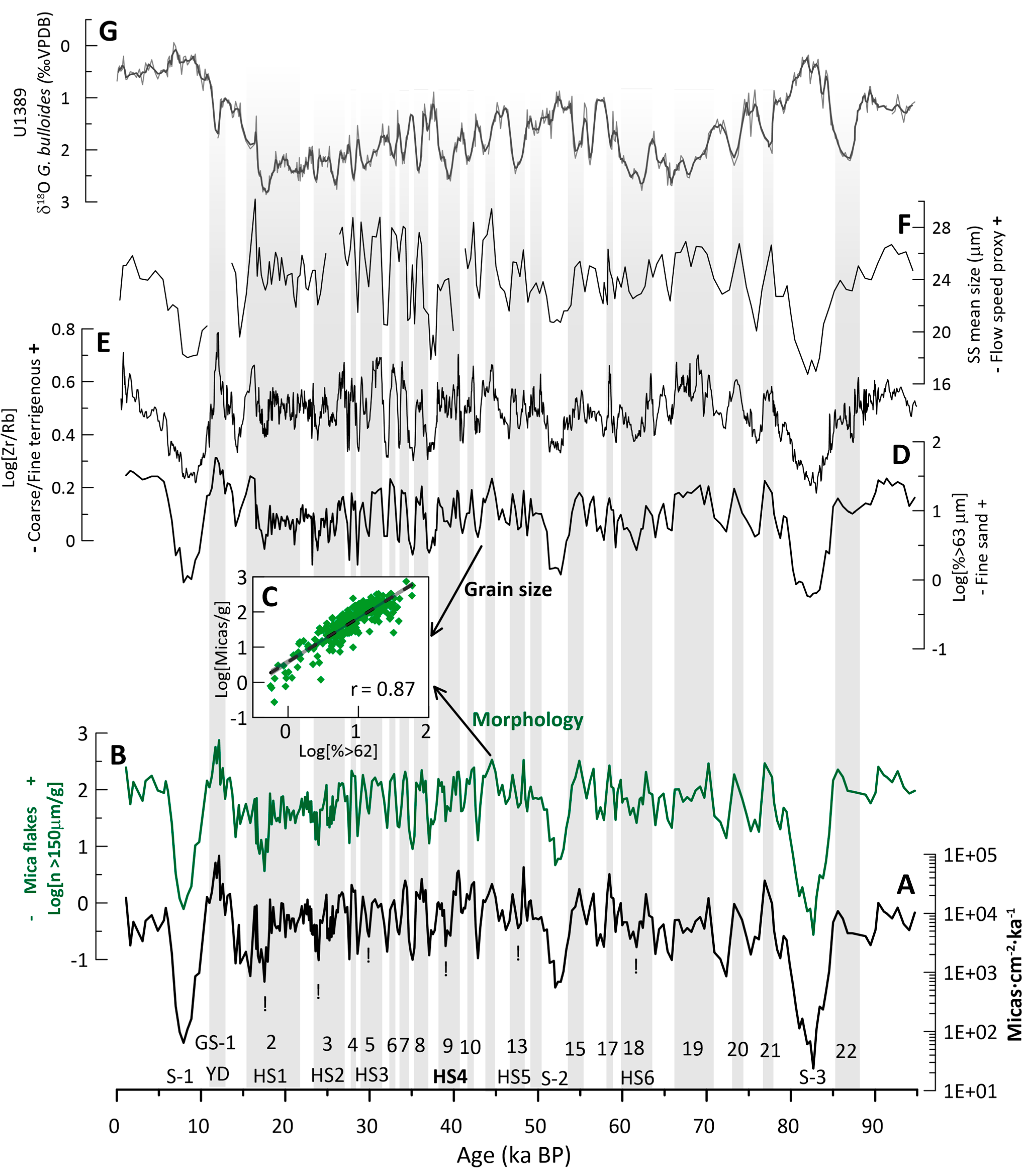
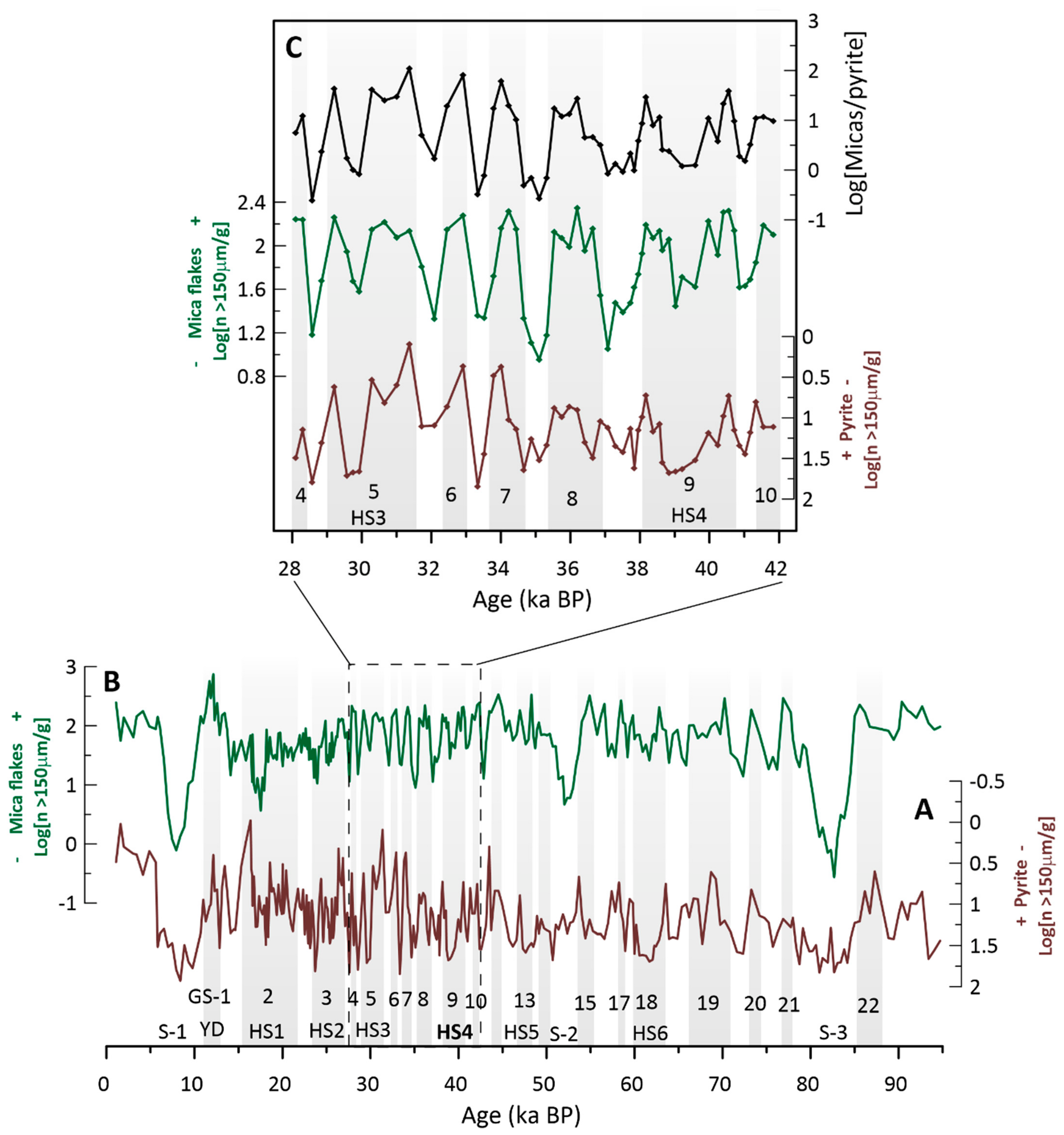
Mica flake content (>150 µm particles/g of dry bulk sediment) shows strong correlation with the proportion of fine sand (r = 0.87 vs. % fine sand) (Figure 3B–D). As for the rest of MOW strength proxies, mica content exhibits relative maxima during Greenland stadial (GS) periods, relative minima during Greenland interstadial (GI) periods, absolute minima during Mediterranean sapropels and the absolute maximum at the Younger Dryas (YD, ~12 ka BP). During Heinrich stadials, mica content exhibits a three-phase structure, in which an event of weaker MOW interrupts the relatively strong MOW stadials (Figure 4C).
Framboidal pyrite content shows an overall inverse correlation with MOW strength proxies and mica flakes. It exhibits relative minima during GSs and relative maxima during GIs and Mediterranean sapropels (Figure 4A).

3.2. Sortable Silt Residuals

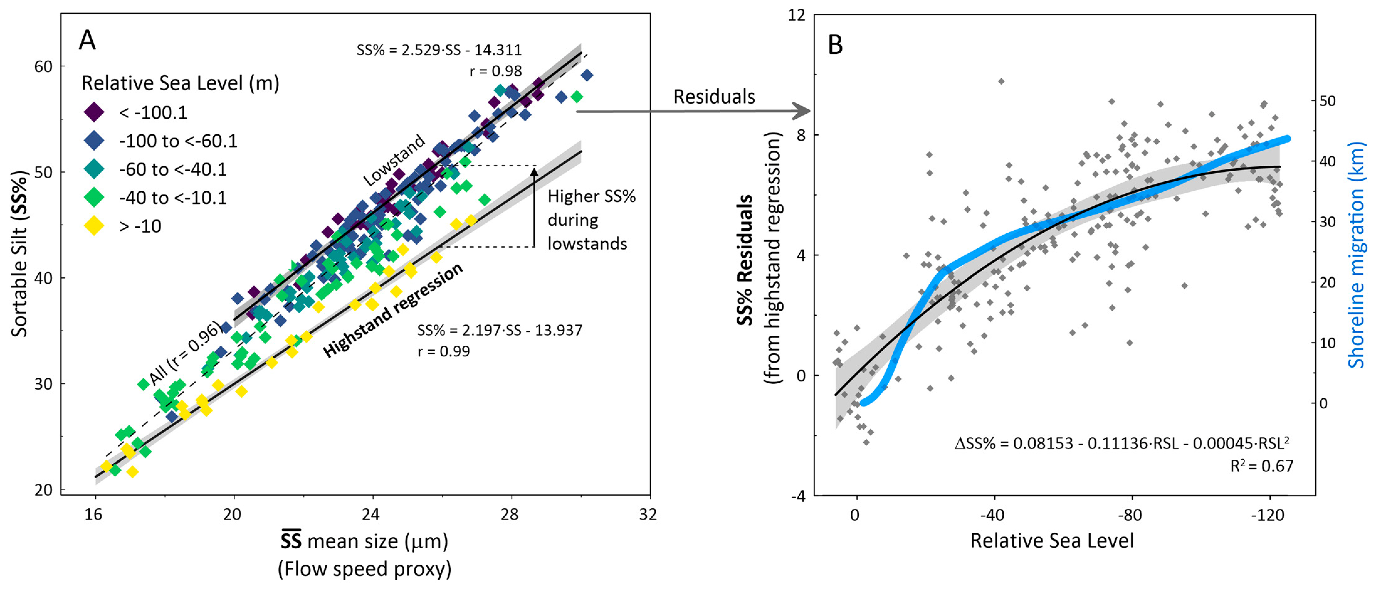
S S ¯ shows strong correlation with SS% for the Late Pleistocene (r = 0.96; Figure 5A). When representing RSL correspondence for each sample, lowstands display higher SS% for a given S S ¯ . Linear regression for Late Pleistocene highstands is as follows:
SS % = 2.197 S S ¯ 13.937   ( r = 0.99 ;   p < 0.0001 ; n = 28 )   ( Figure   5 A )
Linear regression for the Late Pleistocene lowstand (LGM) is as follows:
SS % = 2.519 S S ¯ 14.311   ( r = 0.98 ;   p < 0.0001 ; n = 46 )   ( Figure   5 A )
SS% residuals from highstand linear regression are compared to the coeval RSL and related shoreline migration (Figure 4B). The 2-degree polynomial fitting for the SS% residuals vs. RSL scatter is as follows:
SS% = 0.08153 − 0.11136RSL − 0.00045RSL2 (R2 = 0.67; p < 0.0001) (Figure 5B)
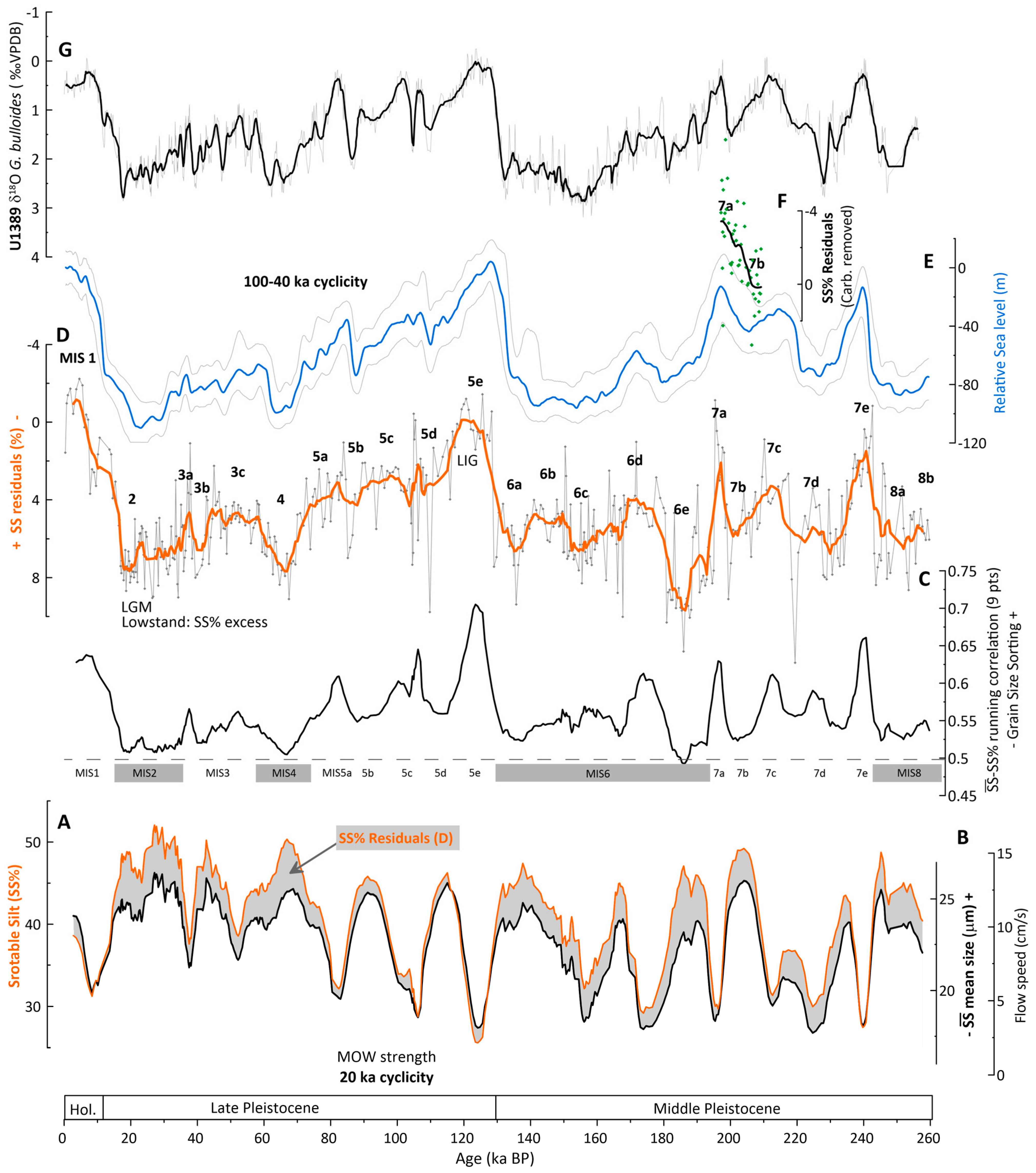
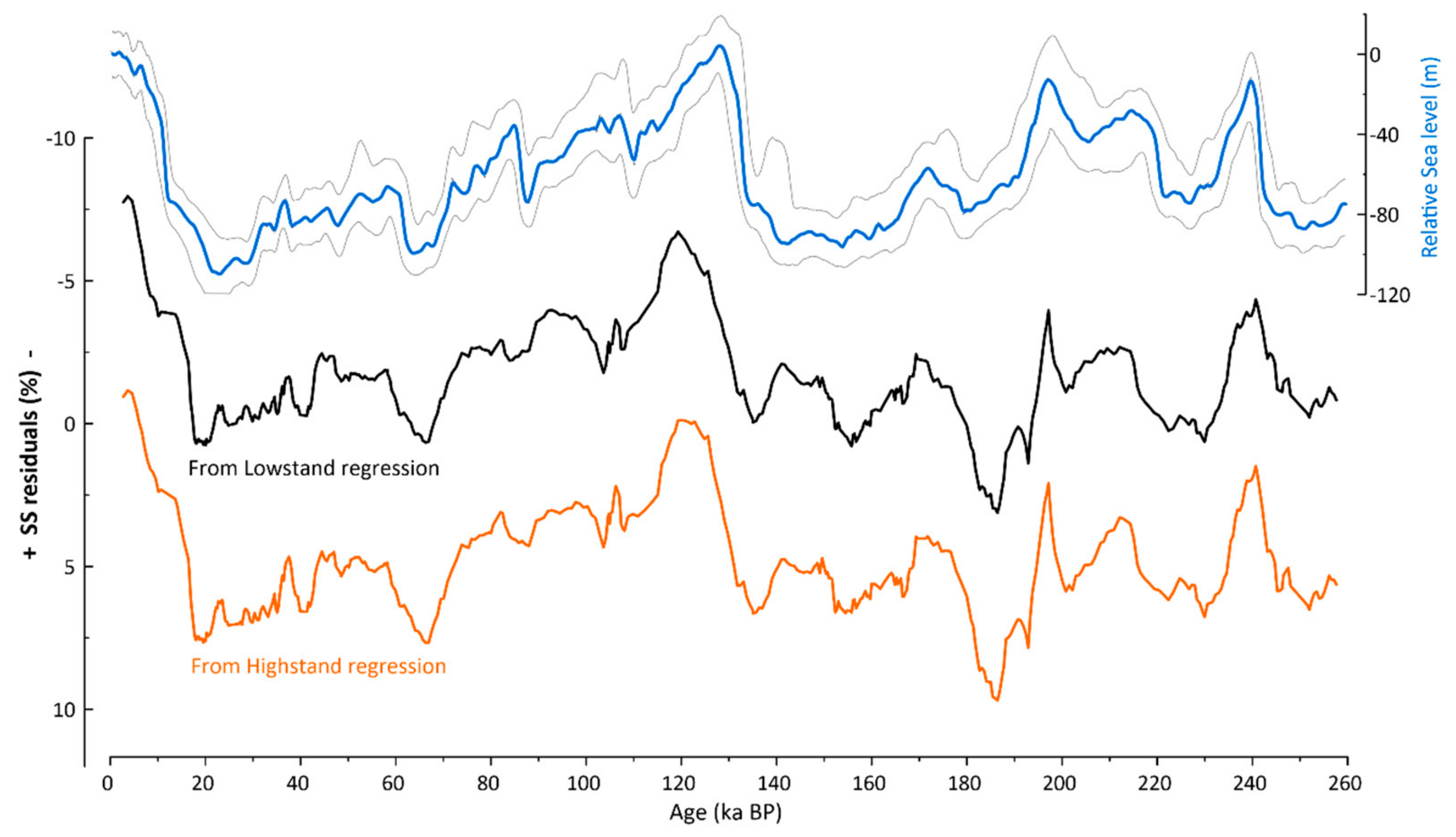
The timeseries of SS% residuals from highstand regression correlate with the RSL curve [36] over the last 260 ka (Figure 6D,E), marking all the correspondent Marine Isotopic Stages (MISs) and substages as defined by [39]. Glacial maxima (lowstands) are characterized by an SS% excess of approximately 8% with respect to the highstand regression from Figure 5A. SS% residuals from the lowstand regression in Figure 5A exhibit similar trends (Figure A1). The 9-sample running correlation of S S ¯ –SS% is >0.5 throughout the record, displaying lower values during lowstands (even MISs) (Figure 6C). SS% residuals display maximum values of ~10% during MIS 6e (~180–190 ka BP), corresponding to the minimum running S S ¯ –SS% correlation (Figure 6C).
The SS% residuals of the carbonate-free dataset spans from MIS 7a to MIS 7b (~195–210 ka BP [39]) and exhibit a decreasing trend with ΔSS% = 4% (Figure 6F), similar to that observed in non-carbonate-free residuals over the same period.

3.3. Spectral Analyses

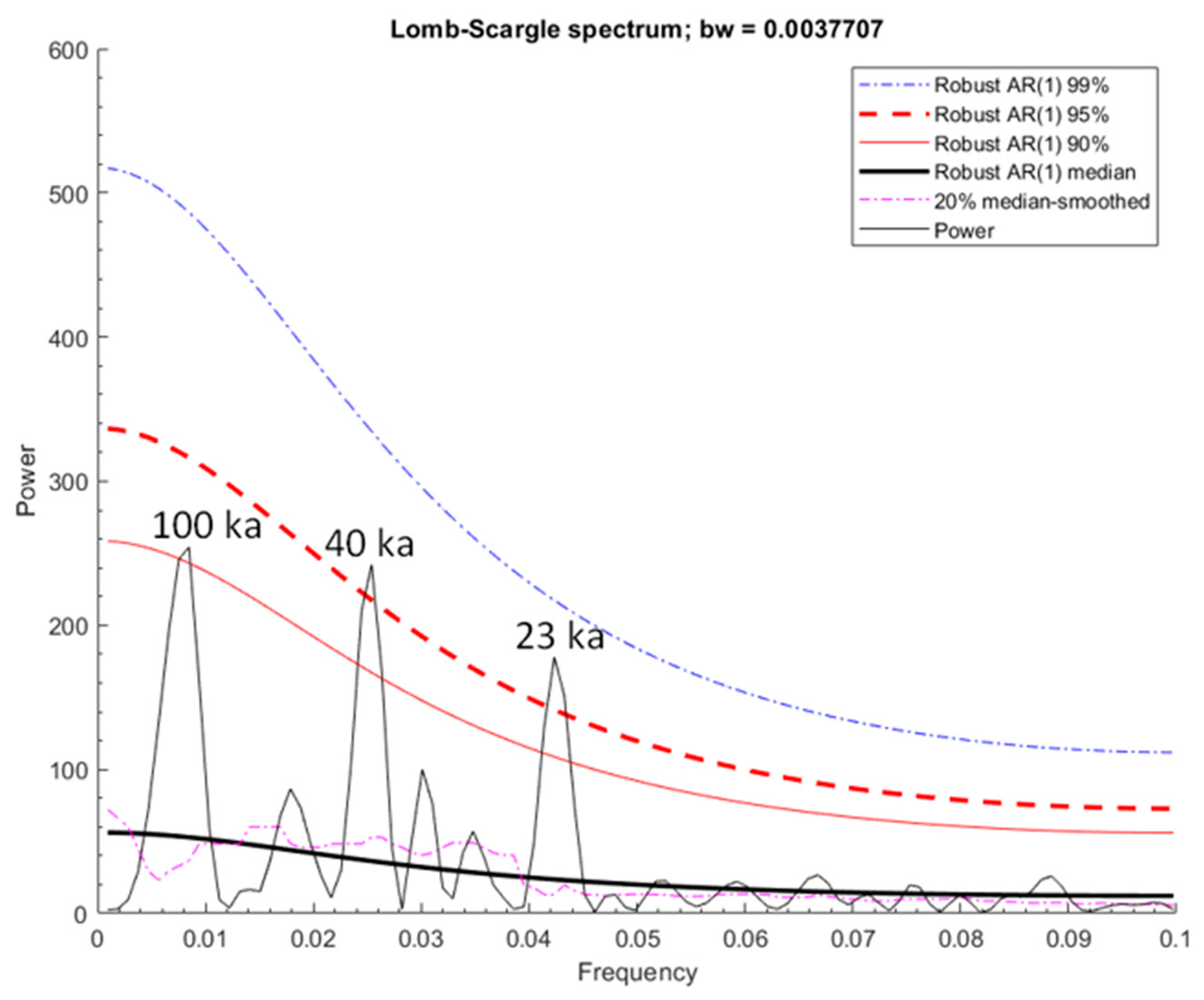
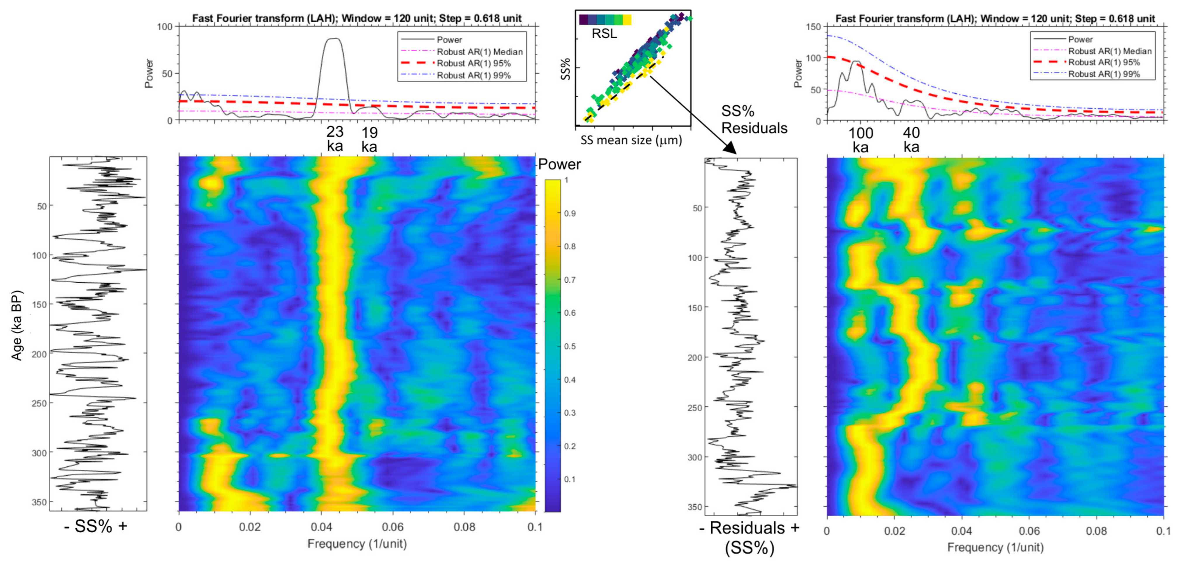
The SS% record from [5] exhibits a dominant and significant 20 ka cyclicity (power above the 99% AR significance level) over the last 360 ka, as previously reported by [5]. The SS% residuals after highstand regression from Figure 5A exhibit dominant, significant 100 ka periodicity (power > AR 95%) over the last 360 ka (Figure 7). Evolutionary spectral analysis indicates that these cyclicities are consistent throughout the record. Spectral analysis for the last 265 ka (age model from [2]) exhibits significant periodicities at 23 ka (precession), 40 ka (obliquity) and 100–120 ka (eccentricity) (Figure A2).

4. Discussion

4.1. Allogenic and Authigenic Minerals as MOW Strength Proxies

Strong correlation between >150 µm mica content, the >63 µm fraction, and the rest of MOW strength proxies (Figure 3) highlights the sensitivity of these particles to bottom current activity. The latter property is well known, as micas and other platy particles have been used to identify current-influenced depositional environments [40]. Owing to their platy shape (Figure 2), mica flakes serve as proxies for finer grain size fractions, exhibiting hydrodynamic drag equivalent to that of a quartz grain approximately ten times smaller in size [41]. Therefore, the concentration of sand-sized mica flakes would be proportional to the sortable silt fraction. Mica content may be biased by the diluting effect of major sediment components (primary productivity, terrigenous supply). Mica flakes, as individual counting features, can be expressed in flux units thanks to the well-constrained age model, thereby minimizing the effects of sediment dilution (Figure 3A).
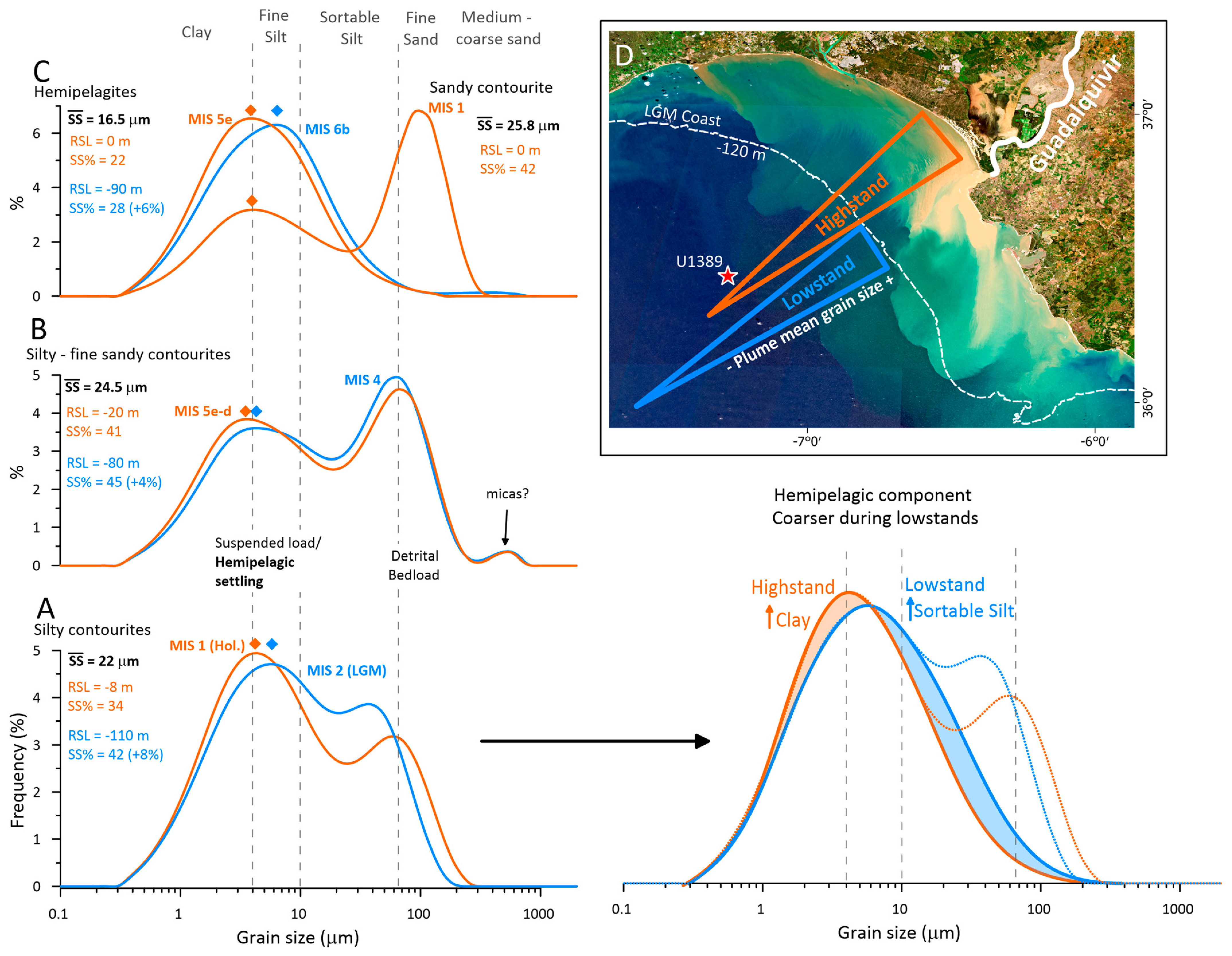
The high sensitivity of mica abundance to bottom current activity makes micas a valuable proxy that records subtle changes during periods of weak bottom current activity, such as those associated with Mediterranean sapropel events. During Mediterranean sapropel S3 (~83 ka BP), the minimum mica content is more pronounced than that observed in the fine sand fraction and coincides with the minimum Ln[Zr/Rb], an established MOW strength proxy [4] (Figure 3E). Mica flakes, as a detrital component of unique hydrodynamic behavior, may also bias the grain size distribution. Most silty contourite samples exhibit a subtle peak in the sand size range, located approximately one order of magnitude above the sorted component peak, which may be attributed to the presence of mica flakes (and bioclasts) (Figure 8B).
Pyrite, as an authigenic mineral, is not directly related to bottom current strength. The precipitation of this iron sulfide is controlled by a complex combination of variables on the seafloor. Authigenic pyrite is generally induced by the biogenic reduction of sulfates under euxinic, anoxic or dysoxic conditions within the upper centimeters of sediment [42]. Hence, organic matter flux and preservation, dissolved oxygen, temperature, Fe availability, grain size distribution and other variables interact to promote pyrite precipitation [43]. At IODP Site U1389, several variables that promote pyrite precipitation are inversely correlated to MOW strength: the bottom current activity of MOW winnows fresh organic matter from export productivity and fine particles, as evidenced from the massive accumulation of coccoliths occurring only during sapropel periods [2], despite relatively low surface productivity [44]; MOW strength is closely linked to Mediterranean ventilation, and therefore dissolved oxygen, which inhibits pyrite formation, is expected to be proportional to MOW strength; and MOW strength, via grain size sorting and winnowing, promotes coarse-grained sediments, with connected pore-waters that inhibit oxygen depletion and pyrite formation.
Rising pyrite content is also a common feature in the Eastern Mediterranean during sapropel deposition [43,45]. Nevertheless, previous studies highlighted that Mediterranean ventilation influences not only pyrite concentration but also its grain size and morphology. A detailed interpretation of the pyrite content record, attending to its formation conditions, remains beyond the scope of this study. Our results indicate that pyrite content is, overall, inversely correlated with MOW strength, although this relationship may arise through different mechanisms. Pyrite registers certain changes with apparent high precision, such as the three phases described for Heinrich stadials [2], in which a relatively low-MOW-strength event disrupts the relatively high MOW strength characteristic of Greenland stadials (Figure 4C).
Since mica and pyrite concentration (n/g) may be affected by dilution from other sediment components, while fluxes (n×cm−2×ka−1) depend on sedimentation rates and thus the accuracy of age models, we propose the authigenic/allogenic (mica/pyrite) ratio. As discussed above, the correlation between mica and MOW strength is as straightforward as with the rest of detrital content, and the pyrite–MOW correlation appears to be more complex. The proposed mica/pyrite ratio combines two mineral components that are independent of the biogenic fraction and are related to MOW activity. The use of ratios is intended to minimize the influence of dilution and age model uncertainties, following a similar approach to that commonly used for XRF major element ratios. Thus, the mica/pyrite ratio may provide a complementary proxy for MOW strength variability, subject to further validation through studies in other locations.

4.2. The RSL Imprint on Grain Size Distribution

Previous studies suggested that RSL influences MOW strength by varying sill depth at SoG, which increases density contrast between Mediterranean and Atlantic water masses [5,46] and hampers the water mass exchange [47]. This RSL control on MOW strength would result in an increase of 1 µm in S S ¯ for every 20 m drop in RSL, superimposed on the main S S ¯ precessional variability [5]. However, this possible RSL influence on MOW strength would affect grain size sorting in terms of the rest of MOW strength variability, following the S S ¯ –SS% correlation [22,29], without explaining the observed S S ¯ –SS% dispersion. Our results show higher SS% values under similar S S ¯ during lowstands. The so-called “source effect” in S S ¯ [20] could explain the observed S S ¯ -SS% dispersion by increasing the availability of coarse sortable silt on the middle slope during lowstands, due to the greater proximity of the shoreline to the shelf edge [20,48]. The source effect in S S ¯ would lead to an underestimation of flow speed with further sediment sources due to the lower availability of coarse silt [20]. However, from S S ¯ –SS% dispersion, the source effect does not play a significant role in S S ¯ , since S S ¯ is relatively higher for a given SS% during highstands (Figure 5A). By contrast, shorter sediment source distance is associated with higher sortable silt fractions. Next, we explain how RSL not only may influence MOW strength by changing the SoG section but also biases the grain size fractions.
Throughout the last 260 ka, SS% residuals are inversely correlated with RSL (Figure 6D–F), which controls the distance between the studied site and Guadalquivir river mouth, the main sediment source of the study area [6,7] (see sediment plume in Figure 8D). Sea level controls the partition of riverine terrigenous material for deposition on the shelf, slope, and abyssal plain, increasing sedimentation rates in the latter environments during lowstands [16]. The increase in terrigenous supply during lowstands is consistent with the relatively high sedimentation rates described in the study area for the last glacial periods [2,11,32], mineral clay composition [6] and the dominance of terrestrial organic matter in U1389 sediments during glacial periods [9].
Mean grain size in river sediment plumes decreases with increasing distance from the river mouth, which has been demonstrated in Mediterranean rivers of comparable size to the Guadalquivir [49]. Differences in grain size distributions between highstand and lowstand samples suggest that the right tail of the fine-grained component of the sedimentation adds extra weight to the sortable silt fraction during lowstands (Figure 8), likely leading to the obtained SS% residuals following the RSL. According to previous studies, the fine-grained component of sedimentation at U1389 is originated from suspended load up to 50 µm, and below 20 µm it mainly corresponds to the background hemipelagic settling dominant in the study area [11]. Considering the potential amplitude of RSL-driven Guadalquivir river mouth migration, we suggest that the terrigenous, hemipelagic component of the sediment shifts toward coarser grain sizes during lowstands, as observed in the proximal areas of sediment plumes. This fine-grained sediment may also arrive to U1389 transported by the MOW from upstream or via nepheloid layers from the shelf edge [50]. Regardless of its origin, the deposition of the fine-grained fraction is subject to MOW (winnowing) weakening. The higher mean grain size of the hemipelagic component and suspended load would lead to the higher contribution of this component to sedimentation under similar MOW speed, which would also contribute to higher sedimentation rates.
The predominantly hemipelagic origin of the SS% residuals is supported by the consistency of the signal throughout the record, even during hemipelagite intervals (as defined by [11]) corresponding to Mediterranean sapropels. During glacial period MIS6 (low RSL), a sapropel deposition occurred in the Eastern Mediterranean, known as “glacial sapropel” S6 [51], leading to a minimum in MOW strength at U1389 [19]. The grain size distributions of samples corresponding to this hemipelagic interval were compared with those of hemipelagite samples of similar S S ¯ from the previous sapropel S5, which occurred during a highstand period (Figure 8C). SS% residual differences were consistent with RSL differences between hemipelagite samples.
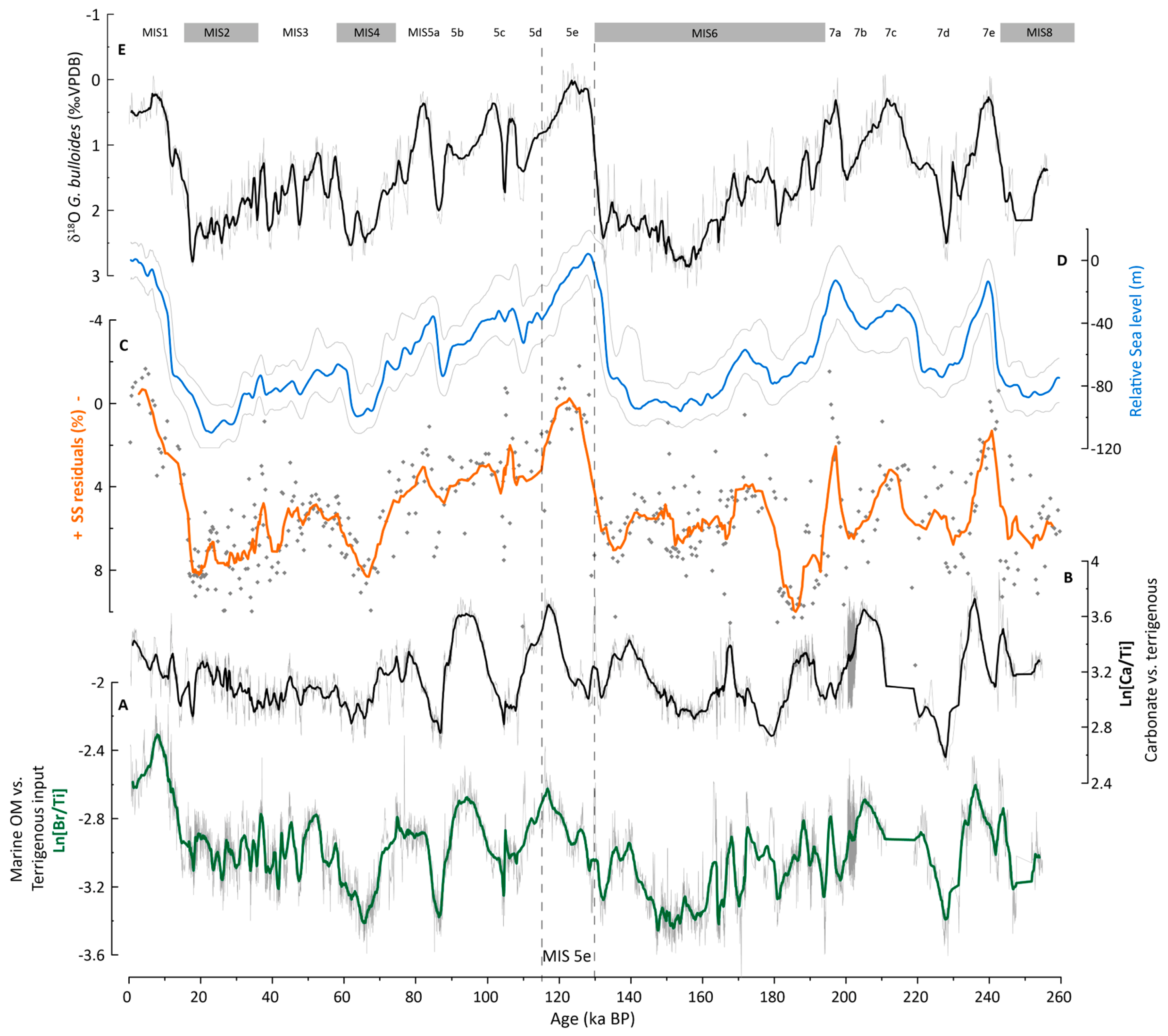
Despite the consistent correlation between SS% residuals and RSL, a contribution from either a lowstand-enhanced pelagic biogenic component (particularly calcareous nanoplankton), aeolian dust or river discharge variability to this proxy cannot be ruled out. SS% residuals from the carbonate-free dataset showed similar trends to those in the bulk sediment SS% residuals (Figure 6F), suggesting that carbonate dilution does not substantially influence SS% residuals. To further explore the possible bias from export productivity, we compared the SS% residuals to the XRF Ca/Ti record, which represents carbonate production vs. terrigenous input [11], and to Br/Ti, which serves as a proxy of marine organic matter accumulation [11,51]. These ratios showed no covariance with the SS% residuals (Figure A3). Regarding aeolian dust, SS% residuals are coherent with RSL across MIS-5, despite marked African humid/dry phases, which were accompanied by pulses of aeolian dust [51]. These African humid periods were almost coeval to the Mediterranean humid periods that affected the Guadalquivir basin [52] and would have been translated into a sediment supply increase. However, coherence across MIS-5 (Figure 6C) suggests that climate (river discharge variability) exerts minor control in SS% residuals compared to RSL. According to the polynomial fitting from SS% residuals vs. RSL (R2 = 0.67; Figure 5B), RSL explains a substantial proportion of the S S ¯ –SS% dispersion.
Once the potential influence of RSL on contourite grain size has been better constrained, future studies could investigate whether variability in river discharge or aeolian input may also influence grain size distributions. The utility of a variable (SS% residuals) that correlates with global sea level curves may extend beyond the interpretation of MOW strength proxies, with potential chronostratigraphic or paleogeographic applications. Applying this approach to other oceanographic settings may provide further insights into its utility and potential broader applicability.

5. Conclusions

Allogenic (mica flakes) content within sandy fractions at IODP Site U1389 shows strong correlation with Mediterranean outflow strength proxies. As a count variable, mica can be used as a MOW strength proxy than can be expressed in flux units. This proxy is based on the laminar grain shape of micas, which makes them proportional to finer detrital fractions. Authigenic (pyrite) content in sediment is overall inversely correlated to MOW strength and can be used in combination with micas to obtain the mica/pyrite ratio, which is presented as a complementary MOW strength proxy.
Sortable silt SS% residuals from S S ¯ /SS% regression may represent RSL-induced sediment supply variability. SS% residuals can be correlated with global RSL curves, displaying an excess of SS% ≈ 8 during glacial maxima. The suggested mechanism underlying SS%–RSL correlation is the relatively coarser terrigenous supply during lowstands that would bring extra sortable silt to the suspended load and the hemipelagic settling. These results may help to interpret past changes in terrigenous supply related to glacial–interglacial sea level changes and the potential influence of these changes on MOW strength records.

Author Contributions

J.P.T.: Conception, writing, figures; F.J.S.: Writing—review, funding acquisition, sample processing. All authors have read and agreed to the published version of the manuscript.

Funding

This research was funded by the contract FPU19/01656 of the Ministry of Universities of Spain awarded to J.P.T. and Project PID 2021-128322-NB-100 (PICTURE) of the Ministry of Science and innovation of the Spain government granted to the Grupo de Geociencias Oceánicas (GGO) of the University of Salamanca.

Data Availability Statement

The following supporting information is available for download at http://doi.org/10.5281/zenodo.20698811 [53]. Raw > 150 µm fraction counts and dry weights, including mica and pyrite content records. SS, SS% and SS% residual records. All additional research data required to reproduce this work is reported in this manuscript.

Acknowledgments

We are very grateful to IODP for providing the samples.

Conflicts of Interest

The authors declare no conflicts of interest.

Appendix A

Figure A1. Comparison of SS% residuals from highstand and lowstand regressions: SS% residuals from highstand regression (Orange) and SS% residuals from Lowstand regression (black). Both highstand and lowstand residuals behave similar regardin RSL variability (in blue; [35]) over the last 260 ka. This similarity is subject to the similar slope of both linear regressions.
Quaternary 09 00065 g0a1
Figure A2. Periodogram of SS% residuals for the last 265 ka BP according to the age model from [2]. All orbital periodicities (eccentricity 100–120 ka; obliquity 40 ka and precession 23 ka) are represented.
Quaternary 09 00065 g0a2
Figure A3. Comparison between SS% residuals and carbonate–export productivity proxies for IODP Site U1389. (A) Br/Ti, proxy for Marine OM accumulation [24,9] (green); (B) Ca/Ti, proxy for carbonate accumulation and principal component of XRF data [24,9] (black); (C) SS% residuals 9 point running average (orange) and data points (gray); (D) Relative Sea Level [36] (blue); (E) Planktic δ18O record from U1389 used for age model tuning [2].
Quaternary 09 00065 g0a3

References

  1. Hernández-Molina, F.J.; Llave, E.; Stow, D.A.V.; García, M.; Somoza, L.; Vázquez, J.T.; Lobo, F.J.; Maestro, A.; Del Rio, V.D.; León, R. The Contourite Depositional System of the Gulf of Cadiz: A Sedimentary Model Related to the Bottom Current Activity of the Mediterranean Outflow Water and Its Interaction with the Continental Margin. Deep. Sea Res. Part II Top. Stud. Oceanogr. 2006, 53, 1420–1463. [Google Scholar] [CrossRef] [Scilit]
  2. Sierro, F.J.; Hodell, D.A.; Andersen, N.; Azibeiro, L.A.; Jimenez-Espejo, F.J.; Bahr, A.; Flores, J.A.; Ausin, B.; Rogerson, M.; Lozano-Luz, R.; et al. Mediterranean Overflow Over the Last 250 Kyr: Freshwater Forcing From the Tropics to the Ice Sheets. Paleoceanogr. Paleoclimatol. 2020, 35, e2020PA003931. [Google Scholar] [CrossRef] [Scilit]
  3. Voelker, A.H.L.; Lebreiro, S.M.; Schönfeld, J.; Cacho, I.; Erlenkeuser, H.; Abrantes, F. Mediterranean Outflow Strengthening during Northern Hemisphere Coolings: A Salt Source for the Glacial Atlantic? Earth Planet. Sci. Lett. 2006, 245, 39–55. [Google Scholar] [CrossRef] [Scilit]
  4. Nichols, M.D.; Xuan, C.; Crowhurst, S.; Hodell, D.A.; Richter, C.; Acton, G.D.; Wilson, P.A. Climate-Induced Variability in Mediterranean Outflow to the North Atlantic Ocean During the Late Pleistocene. Paleoceanogr. Paleoclimatol. 2020, 35, e2020PA003947. [Google Scholar] [CrossRef] [Scilit]
  5. McCave, I.N. One Million Years of Mediterranean Outflow Strength. Quat. Sci. Rev. 2023, 317, 108260. [Google Scholar] [CrossRef] [Scilit]
  6. Moal-Darrigade, P.; Ducassou, E.; Bout-Roumazeilles, V.; Hanquiez, V.; Perello, M.C.; Mulder, T.; Giraudeau, J. Source-to-Sink Pathways of Clay Minerals in the Cadiz Contourite System over the Last 25 Kyrs: The Segregational Role of Mediterranean Outflow Water. Mar. Geol. 2022, 443, 106697. [Google Scholar] [CrossRef] [Scilit]
  7. Campderrós, S.; Pena, L.D.; Garcia-Solsona, E.; Paredes-Paredes, E.; Català, A.; Frigola, J.; Haghipour, N.; Cacho, I. Sediment Provenance and Transport Pathways along the Atlantic Iberian Margin. Earth Planet. Sci. Lett. 2026, 676, 119788. [Google Scholar] [CrossRef] [Scilit]
  8. de Castro, S.; Hernández-Molina, F.J.; Rodríguez-Tovar, F.J.; Llave, E.; Ng, Z.L.; Nishida, N.; Mena, A. Contourites and Bottom Current Reworked Sands: Bed Facies Model and Implications. Mar. Geol. 2020, 428, 106267. [Google Scholar] [CrossRef] [Scilit]
  9. Stow, D.; Smillie, Z.; Wilkin, J.; Pan, J.; Esegbue, O.; Bahr, A.; Ducassou, E. Anatomy of the Bi-Gradational Contourite Sequence: Case Study from the Gulf of Cadiz. Mar. Geol. 2023, 458, 107026. [Google Scholar] [CrossRef] [Scilit]
  10. Lofi, J.; Voelker, A.H.L.; Ducassou, E.; Hernández-Molina, F.J.; Sierro, F.J.; Bahr, A.; Galvani, A.; Lourens, L.J.; Pardo-Igúzquiza, E.; Pezard, P.; et al. Quaternary Chronostratigraphic Framework and Sedimentary Processes for the Gulf of Cadiz and Portuguese Contourite Depositional Systems Derived from Natural Gamma Ray Records. Mar. Geol. 2016, 377, 40–57. [Google Scholar] [CrossRef] [Scilit]
  11. de Castro, S.; Hernández-Molina, F.J.; de Weger, W.; Jiménez-Espejo, F.J.; Rodríguez-Tovar, F.J.; Mena, A.; Llave, E.; Sierro, F.J. Contourite Characterization and Its Discrimination from Other Deep-Water Deposits in the Gulf of Cadiz Contourite Depositional System. Sedimentology 2021, 68, 987–1027. [Google Scholar] [CrossRef] [Scilit]
  12. Mestdagh, T.; Lobo, F.J.; Llave, E.; Hernández-Molina, F.J.; Van Rooij, D. Review of the Late Quaternary Stratigraphy of the Northern Gulf of Cadiz Continental Margin: New Insights into Controlling Factors and Global Implications. Earth. Sci. Rev. 2019, 198, 102944. [Google Scholar] [CrossRef] [Scilit]
  13. Hays, J.D.; Imbrie, J.; Shackleton, N.J. Variations in the Earth’s Orbit: Pacemaker of the Ice Ages. Science 1976, 194, 1121–1132. [Google Scholar] [CrossRef] [Scilit] [PubMed]
  14. Hobart, B.; Lisiecki, L.E.; Rand, D.; Lee, T.; Lawrence, C.E. Late Pleistocene 100-Kyr Glacial Cycles Paced by Precession Forcing of Summer Insolation. Nat. Geosci. 2023, 16, 717–722. [Google Scholar] [CrossRef] [Scilit]
  15. Sierro, F.J.; Ledesma, S.; Flores, J.-A.; Torrescusa, S.; del Olmo, W.M. Sonic and Gamma-Ray Astrochronology: Cycle to Cycle Calibration of Atlantic Climatic Records to Mediterranean Sapropels and Astronomical Oscillations. Geology 2000, 28, 695–698. [Google Scholar] [CrossRef] [Scilit]
  16. Schönfeld, J.; Kudrass, H.-R. Hemipelagic Sediment Accumulation Rates in the South China Sea Related to Late Quaternary Sea-Level Changes. Quat. Res. 1993, 40, 368–379. [Google Scholar] [CrossRef] [Scilit]
  17. Molina, G.S.; Schmiedl, G.; Jiménez-Espejo, F.; Kuhnert, H.; Rodrigues, T.; Voelker, A.H.L. Environmental Changes at the Seafloor of the Faro Drift (Gulf of Cadiz) during the Transition from the Early to the Middle Pleistocene. J. Micropalaeontol. 2026, 45, 117–145. [Google Scholar] [CrossRef] [Scilit]
  18. Llave, E.; Schönfeld, J.; Hernández-Molina, F.J.; Mulder, T.; Somoza, L.; Díaz Del Río, V.; Sánchez-Almazo, I. High-Resolution Stratigraphy of the Mediterranean Outflow Contourite System in the Gulf of Cadiz during the Late Pleistocene: The Impact of Heinrich Events. Mar. Geol. 2006, 227, 241–262. [Google Scholar] [CrossRef] [Scilit]
  19. Sierro, F.J.; Andersen, N. An Exceptional Record of Millennial-Scale Climate Variability in the Southern Iberian Margin during MIS 6: Impact on the Formation of Sapropel S6. Quat. Sci. Rev. 2022, 286, 107527. [Google Scholar] [CrossRef] [Scilit]
  20. McCave, I.N.; Thornalley, D.J.R.; Hall, I.R. Relation of Sortable Silt Grain-Size to Deep-Sea Current Speeds: Calibration of the ‘Mud Current Meter’. Deep. Sea Res. Part I Oceanogr. Res. Pap. 2017, 127, 1–12. [Google Scholar] [CrossRef] [Scilit]
  21. McCave, I.N.; Manighetti, B.; Robinson, S.G. Sortable Silt and Fine Sediment Size/Composition Slicing: Parameters for Palaeocurrent Speed and Palaeoceanography. Paleoceanography 1995, 10, 593–610. [Google Scholar] [CrossRef] [Scilit]
  22. McCave, I.N.; Andrews, J.T. Distinguishing Current Effects in Sediments Delivered to the Ocean by Ice. I. Principles, Methods and Examples. Quat. Sci. Rev. 2019, 212, 92–107. [Google Scholar] [CrossRef] [Scilit]
  23. Bahr, A.; Kaboth, S.; Jiménez-Espejo, F.J.; Sierro, F.J.; Voelker, A.H.L.; Lourens, L.; Röhl, U.; Reichart, G.J.; Escutia, C.; Hernández-Molina, F.J.; et al. Persistent Monsoonal Forcing of Mediterranean Outflow Water Dynamics during the Late Pleistocene. Geology 2015, 43, 951–954. [Google Scholar] [CrossRef] [Scilit]
  24. Bahr, A.; Jiménez-Espejo, F.J.; Kolasinac, N.; Grunert, P.; Hernández-Molina, F.J.; Röhl, U.; Voelker, A.H.L.; Escutia, C.; Stow, D.A.V.; Hodell, D.; et al. Deciphering Bottom Current Velocity and Paleoclimate Signals from Contourite Deposits in the Gulf of Cádiz during the Last 140 Kyr: An Inorganic Geochemical Approach. Geochem. Geophys. Geosystems 2014, 15, 3145–3160. [Google Scholar] [CrossRef] [Scilit]
  25. Stow, D.; Smillie, Z. Distinguishing between Deep-Water Sediment Facies: Turbidites, Contourites and Hemipelagites. Geosciences 2020, 10, 68. [Google Scholar] [CrossRef] [Scilit]
  26. McCave, I.N.; Hall, I.R. Turbidity of Waters over the Northwest Iberian Continental Margin. Prog. Oceanogr. 2002, 52, 299–313. [Google Scholar] [CrossRef] [Scilit]
  27. Hernández-Molina, F.J.; Stow, D.; Alvarez-Zarikian, C.; Expedition, I. IODP Expedition 339 in the Gulf of Cadiz and off West Iberia: Decoding the Environmental Significance of the Mediterranean Outflow Water and Its Global Influence. Sci. Drill. 2013, 16, 1–11. [Google Scholar] [CrossRef] [Scilit]
  28. Stow, D.A.V.; Hernández-Molina, F.J.; Zarikian, C.A.A. Proceedings of the Integrated Ocean Drilling Program; Integrated Ocean Drilling Program Management International, Tokyo: Tokyo, Japan, 2013; Volume 339. [Google Scholar]
  29. Chen, X.; Wu, J.; Pang, X.; Dang, H.; Zhong, L.; Yu, J.; Colin, C.; Liu, Z.; de Lange, G.J.; Kaboth-Bahr, S.; et al. Depth Fluctuations of Mediterranean Outflow Water Along Its Northward Propagation During the Late Pleistocene. Geophys. Res. Lett. 2025, 52, e2025GL116967. [Google Scholar] [CrossRef] [Scilit]
  30. Toucanne, S.; Mulder, T.; Schönfeld, J.; Hanquiez, V.; Gonthier, E.; Duprat, J.; Cremer, M.; Zaragosi, S. Contourites of the Gulf of Cadiz: A High-Resolution Record of the Paleocirculation of the Mediterranean Outflow Water during the Last 50,000 Years. Palaeogeogr. Palaeoclimatol. Palaeoecol. 2007, 246, 354–366. [Google Scholar] [CrossRef] [Scilit]
  31. GEBCO Bathymetric Compilation Group. The GEBCO_2025 Grid—A Continuous Terrain Model for Oceans and Land at 15 Arc-Second Intervals; NERC EDS British Oceanographic Data Centre NOC: Liverpool, UK, 2025. [Google Scholar]
  32. Sierro, F.J.; Flores, J.A.; Baraza, J. Late Glacial to Recent Paleoenvironmental Changes in the Gulf of Cadiz and Formation of Sandy Contourite Layers. Mar. Geol. 1999, 155, 157–172. [Google Scholar] [CrossRef] [Scilit]
  33. Phleger, F.B. Ecology and Distribution of Recent Foraminifera; John Hopkins Press: Baltimore, MD, USA, 1960. [Google Scholar]
  34. Barker, S.; Knorr, G.; Edwards, R.L.; Parrenin, F.; Putnam, A.E.; Skinner, L.C.; Wolff, E.; Ziegler, M. 800,000 Years of Abrupt Climate Variability. Science 2011, 334, 347–351. [Google Scholar] [CrossRef] [Scilit] [PubMed]
  35. Rasmussen, S.O.; Bigler, M.; Blockley, S.P.; Blunier, T.; Buchardt, S.L.; Clausen, H.B.; Cvijanovic, I.; Dahl-Jensen, D.; Johnsen, S.J.; Fischer, H.; et al. A Stratigraphic Framework for Abrupt Climatic Changes during the Last Glacial Period Based on Three Synchronized Greenland Ice-Core Records: Refining and Extending the INTIMATE Event Stratigraphy. Quat. Sci. Rev. 2014, 106, 14–28. [Google Scholar] [CrossRef] [Scilit]
  36. Grant, K.M.; Rohling, E.J.; Ramsey, C.B.; Cheng, H.; Edwards, R.L.; Florindo, F.; Heslop, D.; Marra, F.; Roberts, A.P.; Tamisiea, M.E.; et al. Sea-Level Variability over Five Glacial Cycles. Nat. Commun. 2014, 5, 5076. [Google Scholar] [CrossRef] [Scilit] [PubMed]
  37. Li, M.; Hinnov, L.; Kump, L. Acycle: Time-Series Analysis Software for Paleoclimate Research and Education. Comput. Geosci. 2019, 127, 12–22. [Google Scholar] [CrossRef] [Scilit]
  38. Kodama, K.P.; Hinnov, L.A. Time Series Analysis for Cyclostratigraphy. In Rock Magnetic Cyclostratigraphy; Wiley-Blackwell: Oxford, UK, 2014; pp. 52–89. [Google Scholar]
  39. Railsback, L.B.; Gibbard, P.L.; Head, M.J.; Voarintsoa, N.R.G.; Toucanne, S. An Optimized Scheme of Lettered Marine Isotope Substages for the Last 1.0 Million Years, and the Climatostratigraphic Nature of Isotope Stages and Substages. Quat. Sci. Rev. 2015, 111, 94–106. [Google Scholar] [CrossRef] [Scilit]
  40. Adegoke, O.S.; Stanley, D.J. Mica and Shell as Indicators of Energy Level and Depositional Regime on the Nigerian Shelf. Mar. Geol. 1972, 13, M61–M66. [Google Scholar] [CrossRef] [Scilit]
  41. Doyle, L.J.; Cleary, W.J.; Pilkey, O.H. Mica: Its Use in Determining Shelf-Depositional Regimes. Mar. Geol. 1967, 6, 381–389. [Google Scholar] [CrossRef] [Scilit]
  42. Berner, R.A. Burial of Organic Carbon and Pyrite Sulfur in the Modern Ocean; Its Geochemical and Environmental Significance. Am. J. Sci. 1982, 282, 451. [Google Scholar] [CrossRef] [Scilit]
  43. Passier, H.F.; Middelburg, J.J.; De Lange, G.J.; Böttcher, M.E. Modes of Sapropel Formation in the Eastern Mediterranean: Some Constraints Based on Pyrite Properties; Elsevier: Amsterdam, The Netherlands, 1999; Volume 153. [Google Scholar]
  44. Penaud, A.; Eynaud, F.; Etourneau, J.; Bonnin, J.; de Vernal, A.; Zaragosi, S.; Kim, J.-H.; Kang, S.; Gal, J.-K.; Oliveira, D.; et al. Ocean Productivity in the Gulf of Cadiz Over the Last 50 Kyr. Paleoceanogr. Paleoclimatol. 2022, 37, e2021PA004316. [Google Scholar] [CrossRef] [Scilit]
  45. Passier, H.F.; Middelburg, J.J.; de Lange, G.J.; Böttcher, M.E. Pyrite Contents, Microtextures, and Sulfur Isotopes in Relation to Formation of the Youngest Eastern Mediterranean Sapropel. Geology 1997, 25, 519–522. [Google Scholar] [CrossRef] [Scilit]
  46. Rohling, E.J.; Bryden, H.L. Estimating Past Changes in the Eastern Mediterranean Freshwater Budget, Using Reconstructions of Sea Level and Hydrography. In Proceedings of the Koninklijke Nederlandse Akademie van Wetenschappen (1990); North-Holland Publishing Company: Amsterdam, The Netherland, 1994; Volume 97, pp. 201–217. [Google Scholar]
  47. Rogerson, M.; Rohling, E.J.; Bigg, G.R.; Ramirez, J. Paleoceanography of the Atlantic-Mediterranean Exchange: Overview and First Quantitative Assessment of Climatic Forcing. Rev. Geophys. 2012, 50, RG2003. [Google Scholar] [CrossRef] [Scilit]
  48. Covault, J.A.; Graham, S.A. Submarine Fans at All Sea-Level Stands: Tectono-Morphologic and Climatic Controls on Terrigenous Sediment Delivery to the Deep Sea. Geology 2010, 38, 939–942. [Google Scholar] [CrossRef] [Scilit]
  49. Pitarch, J.; Falcini, F.; Nardin, W.; Brando, V.E.; Di Cicco, A.; Marullo, S. Linking Flow-Stream Variability to Grain Size Distribution of Suspended Sediment from a Satellite-Based Analysis of the Tiber River Plume (Tyrrhenian Sea). Sci. Rep. 2019, 9, 19729. [Google Scholar] [CrossRef] [Scilit] [PubMed]
  50. Lebreiro, S.M.; Antón, L.; Reguera, M.I.; Marzocchi, A. Paleoceanographic and Climatic Implications of a New Mediterranean Outflow Branch in the Southern Gulf of Cadiz. Quat. Sci. Rev. 2018, 197, 92–111. [Google Scholar] [CrossRef] [Scilit]
  51. Ziegler, M.; Tuenter, E.; Lourens, L.J. The Precession Phase of the Boreal Summer Monsoon as Viewed from the Eastern Mediterranean (ODP Site 968). Quat. Sci. Rev. 2010, 29, 1481–1490. [Google Scholar] [CrossRef] [Scilit]
  52. Camuera, J.; Ramos-Román, M.J.; Jiménez-Moreno, G.; García-Alix, A.; Ilvonen, L.; Ruha, L.; Gil-Romera, G.; González-Sampériz, P.; Seppä, H. Past 200 Kyr Hydroclimate Variability in the Western Mediterranean and Its Connection to the African Humid Periods. Sci. Rep. 2022, 12, 9050. [Google Scholar] [CrossRef] [Scilit] [PubMed]
  53. Tarruella, J.P.; Sierro, F. IODP Site U1389 sediment counts (0–55 mcd; 0–95 ka BP) and SS% residuals (0–130 mcd; 0–265 ka BP) [Dataset]. Zenodo 2026. [Google Scholar] [CrossRef]
Figure 2. The >150 µm fractions of two different samples. (A) A sample rich in allogenic mineral particles, mainly mica flakes. (B) A sample rich in authigenic mineral particles (pyrite). A detailed view shows the common framboid morphology of pyrite.
Quaternary 09 00065 g002
Figure 3. IODP Site U1389 MOW strength proxies. (A) The >150 µm mica content expressed as flux (n×cm−2×ka−1). (B) The >150 µm mica concentration in sediment expressed as n/g (this work). (C) The positive correlation between the very fine sand fraction and sandy mica flakes. The gray-shaded area marks the 95% confidence interval. (D) The fine sand proportion [2]. (E) XRF fine terrigenous/detrital content proxy Zr/Rb [24]. (F) Sortable silt mean size (SS) [5]. (G) The planktic δ18O record from U1389 used for age model tuning [2]. Abbreviations refer to Mediterranean sapropels (S-n), Greenland stadials (GSs, gray bands), Heinrich stadials (HSn) and Younger Dryas (YD). Heinrich events 1 to 6 are marked with !.
Quaternary 09 00065 g003
Figure 4. (A) Pyrite content in sediment expressed as Log[n particles/g]. Note that the y-axis is inverted. (B) Mica content in sediment expressed as Log[n/g]. (C) An expanded interval showing stadial–interstadial variability and Log[mica/pyrite]. Numbers refer to Greenland stadials (GSs, gray bands) and Heinrich stadials (HSn), and white intervals correspond to Greenland interstadials (interstadial n comes before stadial n).
Quaternary 09 00065 g004
Figure 5. (A) S S ¯ –SS% correlation (sorting proxy) for the last 129 ka. Linear regressions for RSL highstand (>−10 m) and lowstand (<−90 m) samples are shown. Gray bands indicate 95% confidence intervals for regressions. (B) The distribution of SS% residuals from the highstand linear regression of A with respect to RSL (scatter). The 2-degree polynomial fitting of SS% residuals—RSL (black line and 95% confidence level in gray). Shoreline displacement due to sea level according to present bathymetry is indicated in light blue and the right Y axis.
Quaternary 09 00065 g005
Figure 6. (A) Running average (9 pts) of SS% record [5] for last 260 ka (orange). (B) Running average (9 pts) of sortable silt mean size ( S S ¯ [5] (black). Y axes are scaled proportional to highstand linear regression values from Figure 5A; therefore, distance between curves (gray-shadowed) represents SS% residulas. (C) S S ¯ –SS% 9-sample running correlation as a sorting proxy as defined by [22]; dashed line marks 0.5 threshold. (D) Running average (9 pts) of SS residuals (%) from highstand regression (orange) and individual sample data points (gray). Main Marine Isotopic Stages (MISs) and substages, labeled in black (definition by [39]). Note that Y axis is descending. (E) RSL curve with 95% confidence interval [36] (blue). (F) SS% residuals from regression of carbonate-free samples from [9]. Running average in black. (G) Planktic δ18O record from U1389 used for age model tuning [2]. LGM: Last Glacial Maximum; LIG: Last Interglacial.
Quaternary 09 00065 g006
Figure 7. Spectral and evolutionary spectral analyses of SS% (left) and SS% residuals from highstand regression (right). Note that this interval includes the age model from [5].
Quaternary 09 00065 g007
Figure 8. The grain size distribution of several pairs of samples with equal sortable silt mean size (indicated as S S ¯ in µm). Grain size data from [5,8]. Orange curves represent the relatively high RSL sample, blue curves the relatively low RSL. Diamonds indicate the modal size of the fine-grained component. Note that the fine-grained mode is similar regardless of bottom current speed. (A) Silty contourites with S S ¯ = 22 µm. The possible decomposition of curves is shown on the right. (B) Fine sandy contourites with S S ¯ = 24.5 µm. (C) Hemipelagites corresponding to Mediterranean sapropel periods with S S ¯ = 16.5 µm and sandy contourite with S S ¯ = 25.8 µm; the fine-grained, hemipelagic component of the sediment is shifted to the right during lowstands, adding coarser (sortable silt) particles. The lowstand shift in the hemipelagic component to coarser values can explain the SS% residuals and the strong correlation to the RSL curve. (D) A partial explanation of SS% residual changes between highstand and lowstand periods through river sediment plume grain size. The satellite image from 14 February 2026 illustrates the sediment plumes of the Guadalquivir river approaching the U1389 site (red star) (Sentinel-2; Copernicus EO browser) https://apps.sentinel-hub.com/eo-browser/ (accessed on 16 April 2026).
Quaternary 09 00065 g008
Disclaimer/Publisher’s Note: The statements, opinions and data contained in all publications are solely those of the individual author(s) and contributor(s) and not of MDPI and/or the editor(s). MDPI and/or the editor(s) disclaim responsibility for any injury to people or property resulting from any ideas, methods, instructions or products referred to in the content.