Article

Climate During the Last Glacial Maximum in the Southern Sangre de Cristo Mountains, Colorado, U.S.A.

1
Geology Discipline, University of Minnesota, Morris, MN 56267, USA
2
Integrated Terrain Analysis Program, Division of Earth and Ecosystem Sciences, Desert Research Institute, Northern Nevada Science Center, Reno, NV 89512, USA
3
Department of Geology and Geophysics, University of Utah, Salt Lake City, UT 84112, USA
*
Author to whom correspondence should be addressed.
Quaternary 2025, 8(4), 64; https://doi.org/10.3390/quat8040064
Submission received: 7 August 2025 / Revised: 22 September 2025 / Accepted: 13 October 2025 / Published: 3 November 2025

Abstract

Reconstruction of seven paleoglaciers in the southern Sangre de Cristo Mountains of Colorado formed the basis of temperature-index modeling to estimate the magnitude of temperature change during the Last Glacial Maximum (LGM). The model is used to determine temperatures and precipitation that would maintain steady-state mass balance of the glaciers at their maximum LGM extents. If precipitation was similar to that today, modeling suggests that LGM mean annual temperatures were between ~8.9 and 10 °C cooler, with associated uncertainties of ±1 °C. Modest increases in precipitation (i.e., 100 mm yr−1) that are indicated by some climate modeling do not appreciably lower the magnitudes of temperature depression required for steady-state mass balances. While these new estimates of temperature depression in the Colorado Rocky Mountains align with some that were similarly derived, they are significantly greater (cooler) than others. However, they are consistent with regional-scale climate models as well as high-resolution downscaling of global LGM climate for the Sangre de Cristo.

1. Introduction

The Last Glacial Maximum (LGM; ~26.5–19 thousand years, or ka [1]) represented an extreme climate state in Earth’s past. Knowledge of LGM climate is therefore fundamental for understanding climate dynamics that ultimately informs model projections of future climate change. This knowledge has largely relied on pollen spectra and other microfossils, speleothem records, lake level reconstructions, and so forth. These proxies in and of themselves are important in understanding paleoclimate dynamics, but also because they constrain regional scale climate modeling, particularly in the western United States [2,3,4,5]. Yet while forming the core of available climate proxies, these often do not yield quantitative measures of climatic parameters. More significantly, some proxies begin some time after and thus do not strictly record LGM climate.
Alternatively, modeling of mass balances of paleoglaciers has provided quantitative estimates of LGM climate in the Rocky Mountains [6,7,8,9,10,11,12,13,14,15,16,17]. In general, temperatures and/or precipitation are sought that maintain steady-state mass balances of paleoglaciers at their LGM extents using difference approaches. These include more physically based coupled energy/mass balance and ice flow models [6,7,8,9,10,11,12] and more empirical temperature-index modeling [13,14,15,16,17]. While these approaches have in some instances differed on the precise magnitude, they suggest an LGM temperature depression of ~5 to 9 °C cooler than the present. However, most studies have focused on glaciated ranges in Utah, Wyoming, and northern and central Colorado; few studies [8,10,16] have examined the most southerly regions of the Rocky Mountains region. Moreover, temperature depression in the southernmost Sangre de Cristo Mountains in New Mexico appears to be cooler than expected [10] from that suggested by climate modeling (e.g., Oster et al., 2015 [2]; Lora and Ibarra [5]; Shafer et al., 2021 [18]) that show a consistent north-to-south decrease in cooling along the Rocky Mountains.
Accordingly, it is clear that our understanding of paleoclimate over the southern extent of the Rocky Mountains would benefit from additional estimates of LGM temperature depression. These would add to the existing sparse record of late glacial climate change and thus better constrain regional climate simulations. Thus, in this paper we provide another estimate of LGM temperature depression in the southern Sangre de Cristo Mountains in Colorado based on glacier reconstruction and temperature-index modeling.

2. Regional Setting

2.1. Geologic and Geomorphological Setting

Forming a prominent physiographic barrier, the fault-bounded Sangre de Cristo Mountains extend from south central Colorado south-southeast into northern New Mexico (Figure 1). Rocks of the region include Proterozoic igneous and metamorphic basement and Paleozoic through Cretaceous sedimentary sequences. Overall, the structural history of the range is complex, involving deformation through the Late Paleozoic to the present. The range is bounded on the west by the Rio Grande Rift that became active as early as the Miocene [18]. To the east lies the Wet Mountain Valley, to the north a down-faulted block, and southward the downwarped trough of the Raton Basin [19].
Rising some 1000 to over 1500 m above the adjacent valleys, the crest of the Sangre de Cristo consists of numerous peaks exceeding 4000 m (all elevations referred to herein are meters above sea level). Ongoing tectonism has resulted in deeply incised and steep valleys. Presently no glaciers exist in the study area, but many valleys exhibit features of alpine glacial erosion and deposition of the last, or Pinedale, glaciation (ca. ~23–14 ka, corresponding to the LGM and Marine Isotope Stage (MIS) 2) and to some extent the penultimate Bull Lake glaciation (ca. 200–130 ka, MIS 6). Scant evidence exists for a pre-Bull Lake glaciation [20]. Rock glaciers, possibly still active, and other periglacial landforms are common in cirque basins. Valley mouths are deeply incised owing to continued tectonism of the Rio Grande Rift and are fronted by well-developed alluvial fans with surfaces indicating multiple stages of development [21,22].

2.2. Modern Climatology

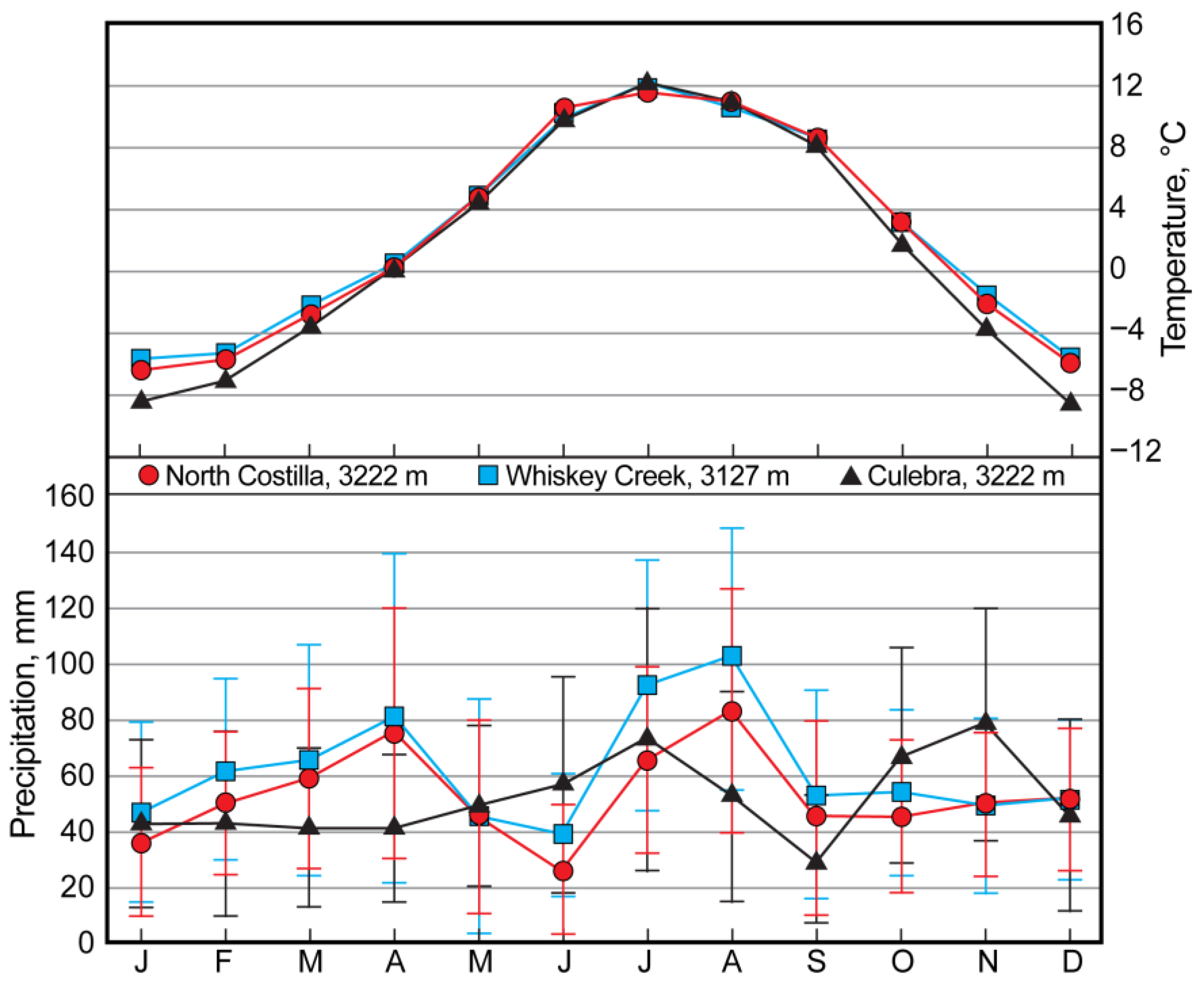
Existing meteorological stations within the study area are limited to elevations (<~2700 m) that are below those of glacier extents. Modern climate is therefore characterized in the model by the PRISM gridded climatology (Parameter-elevation Regressions on Independent Slopes Model; http:/www.prism.oregonstate.edu (accessed on 6 March 2025); [23]) augmented with data from three Snow Telemetry (SNOTEL) stations all located at similar higher elevations (Figure 1 and Figure 2). Median values of 1990–2020 normals are used here. Mean annual precipitation at the highest elevations (~4000 m) is ~1000 mm, decreasing to about half that at valley mouths (~570 mm at ~2900 m).
SNOTEL data are representative of the monthly variation in precipitation (Figure 2). Stations on the eastern slopes (North Castilla and Whiskey Creek) show fairly distinct peaks in precipitation during mid-spring and summer, the latter being more pronounced. This peak is not present in the Culebra SNOTEL record on the western slope. This suggests that the mid-spring peak is possibly related to either late winter/early spring upslope precipitation events over the eastern slopes [24,25] or a result of snow advection by the prevailing westerlies augmenting snow accumulation on eastern slopes [26]. The summer peak in precipitation, evident in all three records, presumably reflects the influence of the summer monsoon [27] that brings subtropical moisture from the Pacific Ocean and Gulfs of California and Mexico. Regionally within the study area, the PRISM data (1991–2020 normals) indicate that eastern slopes annually receive ~150–200 mm more precipitation over elevations between 3000 and 4000 m, this difference increasing with elevation. Precipitation dependence on elevation, a critical aspect of the modeling pursued here, is statistically significant; all correlation coefficients (r2) exceed 0.89 with the number of PRISM gridpoints n used to develop the regressions varying between 45 and 187 depending on the valley or location of interest.
Maximum summer and minimum winter temperatures are typically ~15 and −3 °C, respectively, in valleys, and about ~8 and −11 °C at the highest elevations in the study area. Temperatures strongly vary linearly with elevation, with r2 values all > 0.95 (again, n = 45 to 187). Seasonal temperature variations (January to July) are on the order 18 to 20 °C and relatively constant, but in some valleys show some dependence on elevation. No appreciable differences in seasonal temperature variations are evident over eastern and western slopes as exemplified by the SNOTEL records (Figure 2).

2.3. Timing of the Local LGM

A glacial chronology for the study area has not been established but 10Be exposure ages of boulders on terminal moraines in other areas of the Sangre de Cristo Mountains provide a temporal setting for the local LGM. Preliminary exposure ages (Feldman et al., in prep.) from moraines in Long Valley, New Mexico, about 25 km south-southwest of the study area, suggest that glaciers in that valley reached their maximum extent at ~24.5 ± 1.6 ka. In the Winsor Creek valley, also in New Mexico, about 150 km south-southwest, the LGM is dated to 21.2 ± 2.0 ka [11]. In the South Crestone and South Colony valleys of Colorado, approximately 100 km north-northwest of the study area, glaciers advanced to their maximum ~21 ka [9]. Considering these ages in the context of those in other ranges in Colorado [15,16,28,29,30], the timing of the local LGM in the study area was likely ~20–25 ka and consistent with those in the mountains of the western United States [31].

3. Materials and Methods

3.1. Glacier Reconstruction

The LGM ice extents of seven paleoglaciers (Figure 3) were reconstructed using varying combinations of field mapping of glacial features, high-resolution lidar imagery and derived digital elevation models, geological [32,33,34] and topographic maps, and Google Earth® imagery (Version 7.3.6.10441). Private land ownership limited field mapping in some areas, therefore the reconstructions presented here are more reliant on “remote approaches,” especially lidar. Additionally, detailed reconstructions were not undertaken in valleys where ice limits were ambiguous owing to mass movements and possible remobilization of till in terminal and lateral moraines, among other complexities that would increase uncertainties in model results. Ice in these valleys is shown schematically in Figure 3.
Although software exists for paleoglacier reconstructions, ice surface contours were drawn manually with due consideration of ice extent, local flow directions indicated by erosional forms—often subtle on imagery—and general convergent flow in accumulation zones and divergent flow in ablation zones. Contours were adjusted iteratively so that reconstructed ice surface slopes were sub-parallel to those of the valley and to ensure driving stresses τ were between 50 and 200 kPa, values typically associated with modern glaciers [35]. Stresses were calculated using:
τ =   S f ρ g h   s i n α
where ρ is the density of ice, g is gravitational acceleration, h is ice thickness, α is the slope of the ice surface, and Sƒ is a shape factor to account for drag of the valley sides [36]. Surface slopes were averaged over distances of 10h to account for longitudinal stress gradients [35,37].

3.2. The Temperature-Index Model and Its Implementation

The temperature-index model (TM) and the rationale for using this approach (as opposed to energy-balance modeling) have been discussed in greater detail elsewhere [15,16,17], therefore a brief overview is presented here. The net mass balance Bn of a glacier in steady state with climate will be equal to zero; that is, averaged over some years and over its surface area, the glacier is neither gaining nor losing mass. The annual variation of the specific net mass balance, here at a specific elevation z, is
b n z = t 1 t 2 P s t , z + M t , z d t  
where Ps(t,z) is the rate of snow accumulation, M(t,z) the rate of snow or ice melt (ablation) over the glacier’s surface during the interval t1 to t2, taken as the hydrologic year. In practice, Equation (2) is numerically integrated over a monthly time-scale to yield monthly melt that is combined with monthly precipitation. This sum is then integrated over the hydrologic year to obtain the net balance at z.
Monthly melt is calculated by summing daily melt using a melt factor mƒ that empirically relates ablation to mean daily air temperature Td(t,z):
M z , t = m f T d t , z T d t , z > T m 0 T d t , z T m
where Tm is a threshold temperature above which melting occurs. A compilation of measured melt factors for ice (Supplementary Material in [17]) yields mean (and standard deviation) and median values of 7.33 ± 2.7 and 6.7 mm water equivalent (w.e.) °C−1 d−1, respectively (n = 92). Similarly, for snow the values are 4.3 ± 1.8 and 4.0 mm w.e. °C−1 d−1 (n = 61). For the sake of modeling, therefore, the values of mƒ for ice and snow are taken as 7.0 and 4.5 mm w.e. °C−1 d−1 but in subsequent sensitivity analyses these values were allowed to vary by 2.0 mm w.e. °C−1 d−1. In the model, mƒ is initially set for snow until all snow is melted after which that for ice is used. The threshold for melt was set to +1 °C; additional modeling runs used 0 °C.
Daily air temperature as a function of time of year and elevation is
T d z , t = H ( z ) 1 cos 2 π d 365 ϕ 2 k ( z ) T j a n ( z ) T
where H(z) is the difference between mean July and January temperatures (amplitude of the sinusoid), d is the day of the year, ϕ is the phase lag (=0.359 rads), and Tjan(z) is the mean January temperature at elevation z based on the January linear lapse rate obtained by PRISM climate data (r2 ~0.99). In implementing the model, ∆T is the prescribed LGM temperature perturbation. A tuning parameter k(z) is used to adjust the sharpness of the temperature sinusoid so as to minimize the difference between modeled monthly temperatures during the ablation season (May through September) and those from the PRISM data. Because of valley-to-valley differences in climate, especially precipitation, subsets of the PRISM data vary accordingly. H(z), Tjan(z), and k(z) are also specific for each glaciated valley and in the case of SNOTEL station location (see Section 4.2). Note that H and k are given here as functions of elevation, varying linearly, but in some valleys or regions the correlations are weak and therefore modeling was performed with constant (mean) values of these parameters.
Monthly snow precipitation Ps(t,z) is partitioned from modern monthly precipitation Pmod(t,z) and the prescribed change in LGM precipitation ∆P via a continuous temperature-dependent function determined from the SNOTEL records:
Ps(t,z) = ƒ(Tmonth) (Pmod(t,z) +P).
In detail, ƒ(Tmonth) has the form of a logistic curve relating the snow-to-rain ratio to mean monthly temperature and ensures that in some months a fraction of precipitation falls as snow, some as rain rather than all snow or all rain according to a threshold temperature. Modeling runs used the partitioning function based on proximity to a SNOTEL site, but the effect of using different functions was investigated and discussed subsequently.

4. Results

4.1. Glacier Reconstruction and Equilibrium-Line Altitudes

Attributes of the reconstructed paleoglaciers shown in Figure 3 are summarized in Table 1. Driving stresses are within limits of what is observed in modern glaciers. In general, larger stresses are associated with greater ice thicknesses and/or steeper ice surface slopes, the latter following the steepness of subglacial topography in the valleys. Conversely, lower driving stresses are due to thin ice and/or more moderate slopes and are often found near glacier termini.
Of particular note here are the equilibrium-line altitudes (ELAs) derived from area–altitude ratios (AARs). Regardless of the precise value of the AAR, the reconstructions suggest LGM ELAs on the eastern slopes in the study area are slightly more than 100 m lower than those on the west-facing slopes. Similar east–west asymmetries were recognized elsewhere in the Sangre de Cristo Mountains in Colorado [25] and in the Mosquito Range in central Colorado [15] that, like the Sangre de Cristo, is the most prominent topographic barrier for southeasterly derived moisture transport. Today these ranges are subject to upslope precipitation events in the late winter and early spring that bring Gulf of Mexico moisture that often enhances snow accumulation on the eastern slopes [24,25]. If similar events occurred during the LGM, this could have resulted in greater accumulation which would in effect lower equilibrium lines. This apparent difference in ELAs on opposing slopes has also been attributed to wind transport of snow from western to eastern slopes, either by deflation on the former [38] or advection prior to deposition [17,26], and/or by virtue of difference in net radiation. Presumed strengthening of the prevailing westerlies and/or intensification of the winter jet [2,39,40,41,42] during the LGM could potentially lead to greater wind transport and hence accumulation.
However, a mitigating factor for the enhancement of snow accumulation via such mechanisms is glacier growth and its orographic influence on moisture transport and temperatures [43]. In brief, the growth of glaciers on the western windward slopes not only increases snowfall but also can lead to increased albedo, cooler temperatures, and therefore decreased ablation. Conversely, the eastern slopes would be deprived of snowfall and experience warmer temperatures due to reduced albedo and cloud cover, thus increasing ablation [43]. Combined, this would promote lower ELAs on western and higher ELAs on eastern slopes—the opposite of what is observed in this region of the Sangre de Cristo Mountains. Additionally, ice thicknesses in the study area would not have substantially altered orography, leading to a muted, if any, influence on glacier mass balance. Ultimately, given these competing factors, an explanation for the discrepancy in ELAs remains equivocal.

4.2. Temperature-Index Modeling: Model Skill

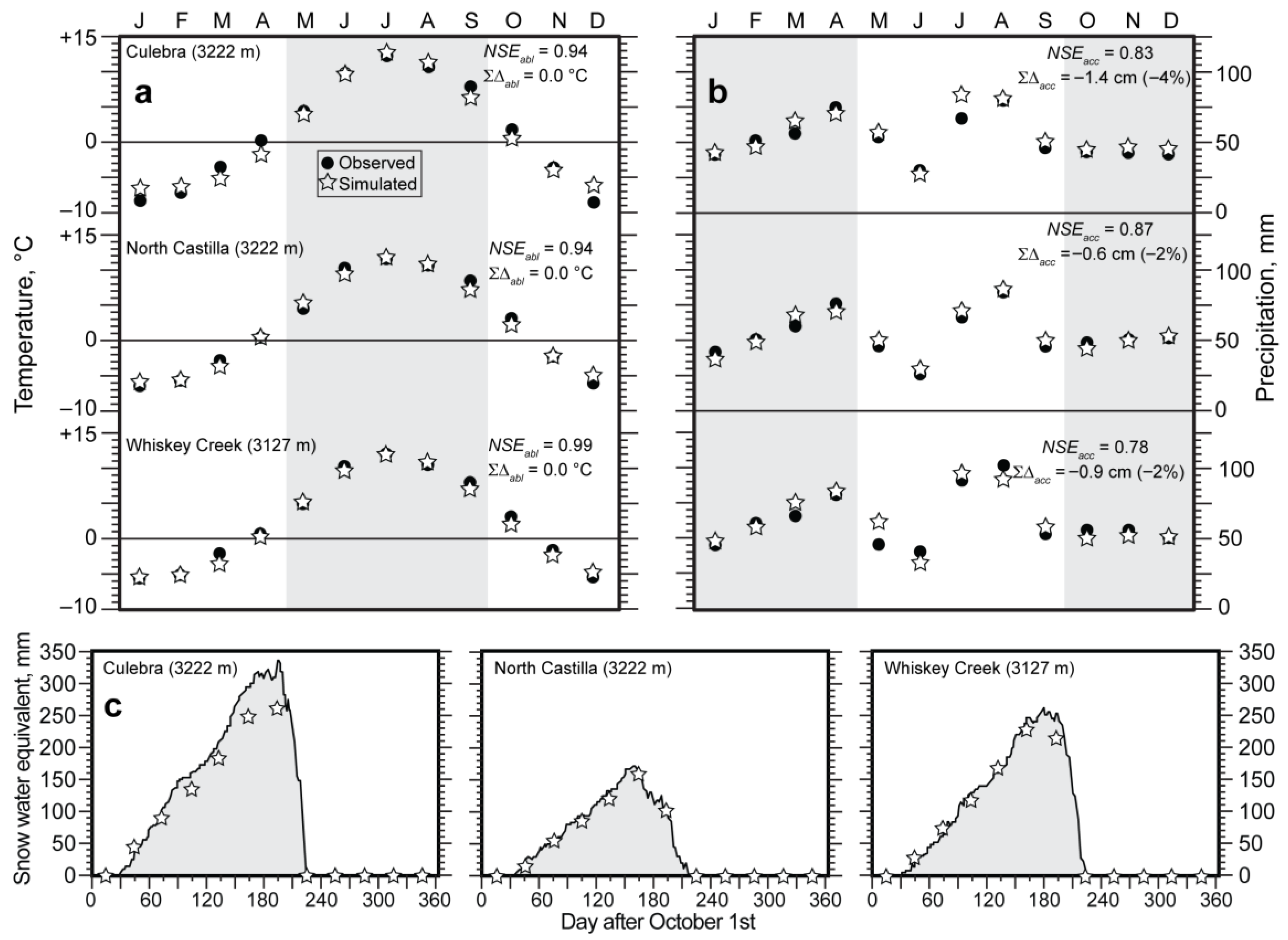
Evaluation of model skill follows the criteria previously used [13,14,15,16,17]: how well the model (1) captures modern climate and (2) reproduces snowpack evolution at SNOTEL stations using parameterization that is unique to the SNOTEL sites. Modeled modern temperatures and precipitation at SNOTEL sites are graphically compared with those observed in Figure 4a,b. For the purpose of modeling, accurate temperatures are most critical during the ablation season (taken here as May through September) and precipitation during the accumulation season (November through April). Cumulative temperature differences during the former are ~0 °C, which is not surprising in view of the fact that the model is tuned (via H(z) and k(z) in Equation (4)) specifically for the SNOTEL locations. Cumulative precipitation differences (no tuning) are very small and negative for all three SNOTEL sites, meaning accumulation season precipitation is very slightly overestimated in the model.
Model–data agreement is also quantified using Nash–Sutcliffe efficiency criteria commonly used in hydrologic modeling:
N S E = 1   i = 1 n ( O i p i ) 2 i = 1 n ( O i O ¯ ) 2
where Oi are the observed values, pi are those modeled, and the overbar denotes the mean of n number of values. A value of 1.0 indicates perfect agreement between modeled and observed values, whereas values approaching or less than 0.0 suggest a poor fit to the observed values. NSE values (Figure 4a,b) are all close to one and thus suggest model results faithfully match the observed SNOTEL data.
Similar comparisons between modeled modern temperatures and precipitation and PRISM values for the valleys of interest are summarized in Table 2. These comparisons are perhaps more significant in that they are more regional in nature and also account for elevational variations in differences. With one exception, modeled temperatures differ from PRISM values by less than 1 °C and on average less than 0.5 °C. NSE statistics for temperature are ≥0.97, indicating nearly perfect agreement. Modeled precipitation values differ by ~10–20 mm or less than 5% of total precipitation. NSE scores for precipitation, with the exception of two, exceed 0.84, indicating good correspondence between modeled and PRISM values. Table 2 also shows that there are no systematic differences, that is, the TM approach neither consistently over- nor underestimates temperature or precipitation.
Finally, modeled snowpack evolution is compared with median 1991–2020 snowpack depth (in snow water equivalent) recorded at the three SNOTEL sites over a hydrologic year (Figure 4c). Here again, PRISM data, the H(z) and k(z) parameters, and snow-to-rain ratio used in the model are specific to each site. Despite differences in temporal resolution (monthly in the model, daily in the SNOTEL records), the agreement is quite good, particularly for the North Castilla and Whiskey Creek sites.

4.3. Steady-State Mass Balances of Paleoglaciers and Implications for LGM Climate

Estimates of LGM climate in the study area were determined by finding temperature and/or precipitation combinations that maintain steady-state mass balances Bn of the reconstructed glaciers, i.e., those that satisfy
B n = A b n d A i = 1 j b n i A i = 0
where bn is the annual specific net mass balance given by Equation (2), A is glacier area composed of j elevation increments, and i denotes the value at an elevation increment, thus glacier hypsometry is explicitly included.
As there are an infinite number of solutions for Equation (7), limits must be placed on possible changes in precipitation in order to obtain estimates of LGM temperature depression. Proxy records of precipitation would serve as such limits, however, such records are sparse in the region and typically do not provide the magnitude of that change. Nevertheless, pluvial lake levels and speleothem records, as well as climate modeling [2,4,44,45,46,47,48,49], point to wetter conditions in the American Southwest during the LGM. Therefore, modeling examined the required temperature depression under imposed increases in precipitation of 100 and 200 mm yr−1 corresponding to ~10–15% and 20–30% increases over modern precipitation, respectively, depending on elevation. It should be noted that paleohydrology of Lake Estancia, about 280 km south-southwest from the study area, suggests possible increases in precipitation at times during the LGM could have been as large as 50 to 100% over modern [36,39], albeit for short intervals of decades. While a number of contrasting mechanisms have been invoked to explain apparent increases in LGM precipitation in the southwest [2,5,50,51,52,53,54,55], the question remains whether these would have affected the study area. In particular, climate models [2,4,5] place the study area at or near the boundary between wetter conditions to the south and drier conditions to the north (the so-called “precipitation dipole”). Thus, in the interest of completeness, additional modeling runs investigate the effect of reducing LGM precipitation by similar amounts.
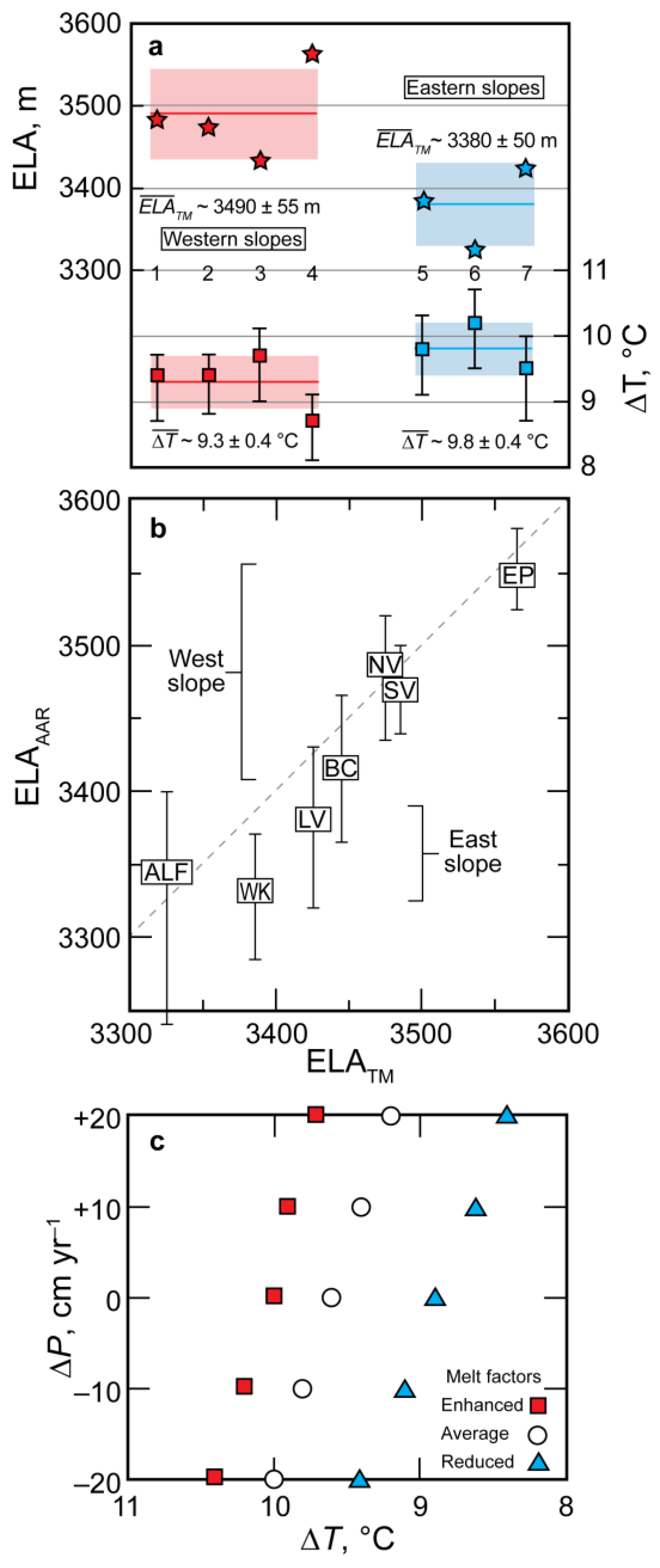
Table 3 and Figure 5a summarize the temperature depression required to maintain steady-state mass balance of the seven paleoglaciers under different scenarios. Assumptions include that LGM precipitation was similar to that today, increased or decreased precipitation, and differences in melt factors. Under the assumption of no change in precipitation and average melt factors, temperature depressions range from 8.7 to 9.8 °C. Figure 5a also shows the associated ELAs from modeling. The individual differences notwithstanding, mean temperature depression appears to be slightly greater, by ~0.5 °C, on the eastern slopes of the study area. Furthermore, ELAs tend to be ~110 m lower on the eastern slopes, consistent with what was noted above for the AAR-derived ELAs. Figure 5b shows ELAs determined by modeling closely agree with using the AAR method. However, given these differences generally fall within estimates of uncertainties (discussed subsequently) and in the interest of determining regional LGM climate, the emphasis here is placed on the (grand) mean temperature depressions of ~9.6 °C for the standard melt scenario and ~8.9 and 10.0 °C for the reduced and enhanced melt scenarios, respectively.
As discussed above, considering the possibility of increased LGM precipitation of 100 mm yr−1 the mean temperature depression to maintain steady-state mass balances is ~9.4 °C, and for 200 mm yr−1 it is ~9.2 °C. In combination with lower melt factors, these temperature depressions could be on the order of ~1 °C less; conversely, with higher melt factors they are ~0.5 °C greater (Table 3) and minimally dependent on these prescribed changes in precipitation (Figure 5c). Decreases in LGM precipitation of 100 mm yr−1 would, on average, require temperatures to be ~9.8 °C cooler than present. A decrease of 200 mm yr−1 would require temperature depressions of ~10.0 °C. Under the reduced and enhanced melt scenarios temperature depressions would be ~0.7 less and ~0.4 °C greater, respectively, and again not strongly dependent on the prescribed changes in precipitation.

4.4. Uncertainties in the Estimates of LGM Temperature Depression

Uncertainties in the TM results were evaluated by performing sensitivity analyses with different model parameters. Specifically, these were parameters in Equation (3): the melt factors mƒ and melt threshold Tm; in Equation (4): k(z)—constant (average value) or non-constant, H(z)—constant or non-constant, the lapse rate Tjan(z); and in Equation (5): ƒ(Tmonth). Additional analyses examine the effect of the melt threshold and glacier hypsometry. Individual uncertainties were added in quadrature. Maximum uncertainties associated with these parameters from each of the seven paleoglaciers, where appropriate, were used to calculate total uncertainty.
Variation in the melt factors for snow and ice yield uncertainties in the estimates of temperature depression of about +0.5/−0.8 °C, corresponding to more or less melt. If the melt threshold is assigned a value of 0 °C instead of +1 °C, required temperature depressions increase by ~0.2 °C. Assuming the tuning parameter k(z) is constant (i.e., a mean value) or not (i.e., a function of elevation) introduces a very small uncertainty less than ± 0.05 °C. Similarly, whether the yearly amplitude in temperature H(z) is assumed constant with respect to elevation or not results in a uncertainties that do not exceed ~±0.3 °C. Reasonable variations in the lapse rate Tjan(z) based on the regressions introduces an uncertainty of ~±0.3 °C. Temperature depressions using different partitioning functions defined at each of the three SNOTEL sites differ by a maximum of ~0.3 °C.
The uncertainties associated with glacier hypsometry are more challenging to assess. Following Brugger et al. [15] a Monte Carlo scheme was used wherein glacier area within elevation intervals was allowed to increase or decrease randomly by 15%; this essentially addresses uncertainties in ice contours as reconstructed and thereby mass balance via Equation (7). This approach suggests uncertainties associated with the hypsometries of the paleoglaciers do not exceed ±0.2 °C. Based on the foregoing the total uncertainty in the estimates of temperature depression is on the order of ±1.0 °C.

5. Discussion

The results of temperature-index modeling suggest that regional LGM temperatures in the southernmost Sangre de Cristo Mountains in Colorado were on the order of 9 to 10 °C cooler even allowing for a modest increase in precipitation. With due consideration of uncertainties, the apparent difference in temperature depression of ~0.5 °C on east- and west-facing slopes (Figure 5a, Table 3) is likely not significant. Nevertheless, the fact that ELAs, determined by both the modeling and using the AAR method, are significantly lower on the eastern slope warrants some attention. As noted above this has been observed elsewhere and possibly reflects less incoming solar radiation, and hence less ablation, and/or any mechanism whereby accumulation is enhanced [17,24,25,26,38] on the eastern slope. Under the assumption that precipitation differences existed during the LGM as they do today, say +100 mm yr−1 on the eastern slope, this difference is reduced, and when combined with the assumption of less ablation (reduced melt scenario), LGM temperatures on the eastern slope would be ~9 °C cooler, again within uncertainties. Thus, the estimates of LGM temperature depression presented here appear to be robust. It bears mentioning that, under these assumptions, TM-derived ELAs on the eastern slope are at most ~20 m higher, thus maintaining accord with those using the AAR approach.
Perhaps the most intriguing result is that of the magnitude of LGM temperature depression. Estimates using a similar TM approach [13,14,15,16,17] and coupled energy/mass balance and flow models [8,9,12] in Colorado show neither a consistency in magnitude nor a coherent spatial pattern (Figure 6). (It should be noted that previous TM modeling referred to here used slightly different melt factors, but this accounts for a difference of ~0.1 °C). For example, in the Front Range of northern Colorado, temperature depression has been estimated to be 4.5 °C assuming precipitation was similar to that today [8]. In contrast, temperature depression over the Blanca Massif in the Sangre de Cristo Mountains may have been nearly twice as large [17] with the same assumption regarding precipitation. This contrast runs counter to the southward decrease in LGM cooling evident in climate models [2,5,18,56], presumably due to less climatic influence of the Laurentide Ice Sheet.
It bears mentioning that this lack of a systematic southward decrease in LGM temperature depression is also evident on a considerably broader latitudinal scale, the paucity of quantitative estimates notwithstanding. Temperature depressions based on glaciological approaches in the Northern Rocky Mountains of Montana [57] range from ~8.5–9.2 °C or ~10.5 °C if drier conditions prevailed. Farther south, in the Central Rocky Mountains of Utah and Wyoming, the same approach yielded temperature depressions that span ~8.5 to 11.5 °C assuming no significant changes in LGM precipitation [11,58,59].
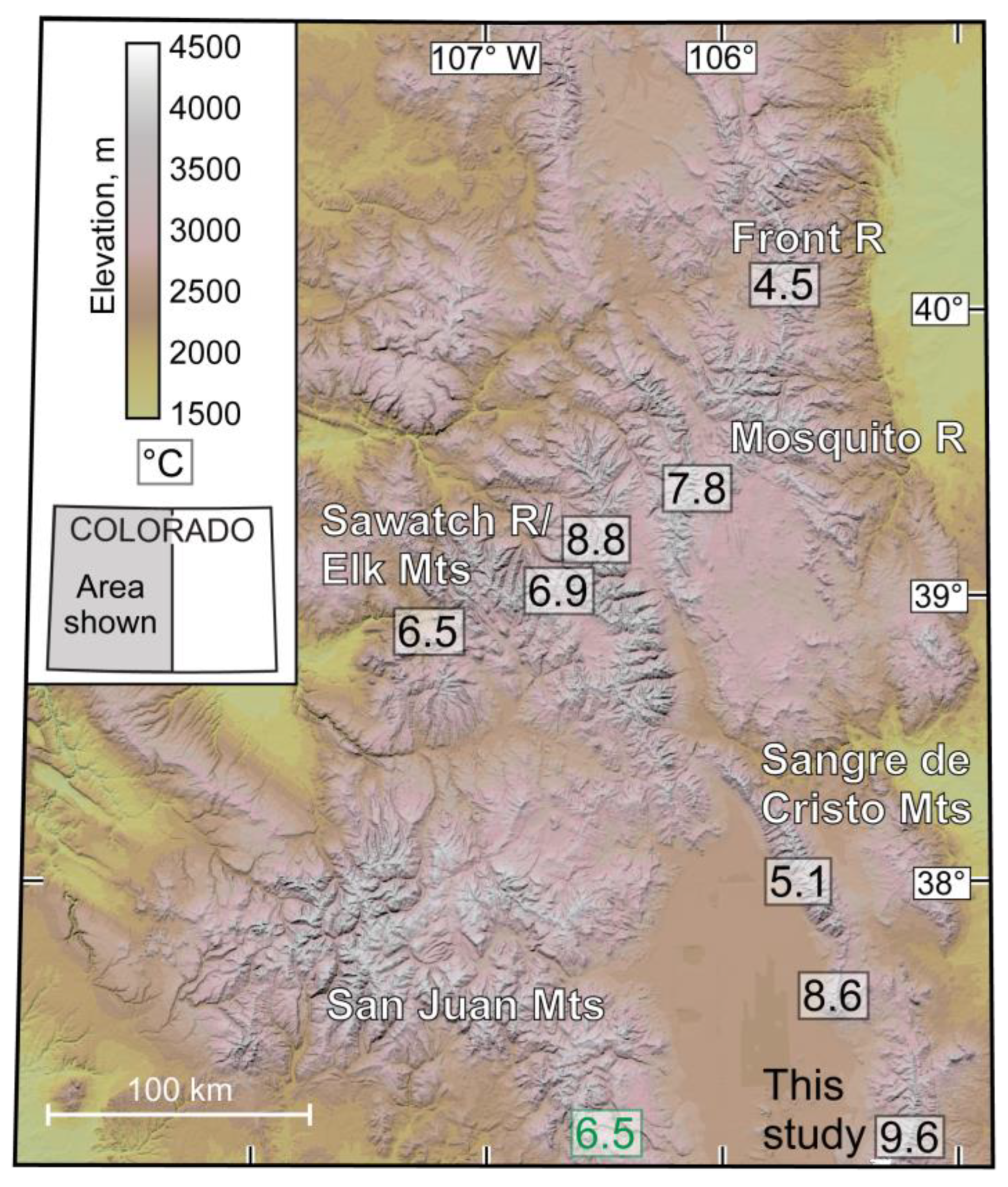
While our estimates of ~9–10 °C appear to support a more severe cooling during the LGM, at least in the Sangre de Cristo Mountains, a temperature depression of ~5 °C has been suggested for the Crestone Peaks region of the range, about 100 km north of the study area [9]. Moreover, recent work [60] using lipid biomarkers in bog sediment in the nearby San Juan Mountains, about 110 km west (Figure 6), yielded an LGM temperature 6.5 °C colder than today. However, (1) basal sediment age was estimated to be ~19.2 ka, potentially predating the LGM in the study area by several thousand years; and (2) this value is the departure from pre-industrial temperatures and therefore probably ~1 °C greater if comparing to modern conditions. Additional support for a colder LGM in the region comes from the southernmost Sangre de Cristo Mountains in New Mexico, where temperature depression was estimated to be 8.6–9.0 °C, providing precipitation was similar to the present, or ~8.0 °C cooler if precipitation was greater than modern [11].
Figure 6. Estimates of LGM temperature depression in Colorado based on glaciological approaches (black) [8,9,12,14,15,16,17]. The values shown here assume LGM precipitation was not different from modern. The estimate shown in green (southern San Juan Mountains) is based on lipid biomarkers [60].
Quaternary 08 00064 g006
The disparate estimates of temperature depression in Colorado (and over the entire Rocky Mountain region) are likely due in part to local modulation of regional climate (i.e., the role(s) of microclimate), differences in the precise timing of local LGM (comparing climate at different times), and/or the particular methodology used to obtain the estimate. But these in and of themselves are not likely to account for such large differences in the measure of LGM climate change. What is not known and therefore somewhat unconstrained in modeling are changes in precipitation that could significantly affect glacier mass balance and consequently temperature depression. This further complicates the picture of regional climate change during the LGM.
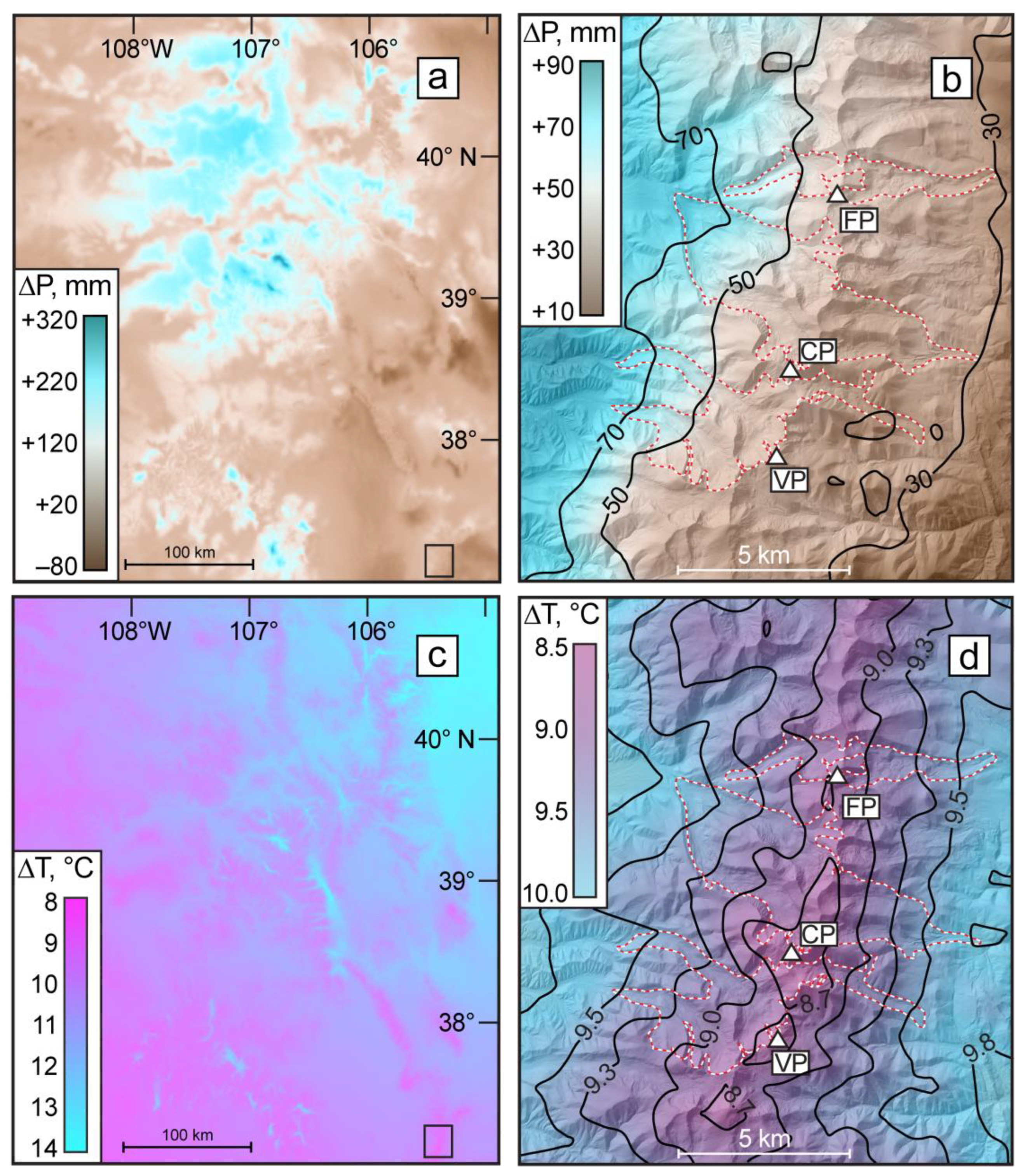
Although the biomarker proxy in the San Juan Mountains [60] is indicative of drier conditions during the LGM, several climate models suggest possible increases in precipitation. An ensemble of nine Paleoclimate Modeling Intercomparison Project Phase 3 [2] (PMIP3) models suggests a mean increase in precipitation within the study area of ~20%, or about 100–150 mm yr−1. However, five of the nine models indicate a reduction of precipitation of similar magnitude, therefore rendering any conclusion with regard to precipitation changes based on PMIP3 models equivocal. More recent Transient Climate Evolution of the last 21k years (TraCE21k) modeling using the downscaling Climatologies at High resolution for the Earth’s Land Surface Area [56] (CHELSA) suggests substantial increases in LGM precipitation in many mountain ranges in Colorado (Figure 7a). In the study area (Figure 7b) more modest increases in precipitation are indicated, on the order of 30 to 70 mm annually. The CHELSA-TraCE21k output also implies a disproportionate increase in precipitation on the western slopes, furthermore suggesting LGM precipitation was more uniform over the study area. This appears to be at odds with the ELA differences on eastern- and western-facing slopes discussed previously. If, however, the greater increase in precipitation on the western slopes resulted from intensification of the prevailing westerlies during the LGM [2,3,4,54,55], this could have also resulted in greater wind drift and/or advection of snow that enhanced accumulation on the eastern slopes. (Obviously, differences in insolation and its effect on local energy balances would factor, at least to some extent, in any explanation of these differences).
Increased precipitation would have the effect of decreasing the magnitudes of LGM temperature depression, particularly in the northern mountain ranges in Colorado. But in the study area the small increase would not significantly affect our results, making it seem more of an outlier. Yet in examining the CHELSE-TraCE21k temperature output, regionally LGM temperatures (Figure 7c) might have been ~8 °C cooler in southwestern Colorado to ~14 °C cooler in the north-central area of the state. In the Sangre de Cristo Mountains (Figure 7d), temperatures appear to have been ~8.5 to ~10 °C colder than present, the change perhaps being more pronounced at lower elevations, possibly due to changes in lapse rates. Such departures from modern temperatures are also corroborated by PMIP3 models that show about an 8.7 ± 2.5 °C cooling in the Sangre de Cristo [2]. Furthermore, using the same approach as that used here, temperature depression on the Blanca Massif just 50 km to the north of the study area averages ~8.6 °C, assuming no change, or ~8.3 °C with a slight increase in precipitation [17].
It is difficult to reconcile this magnitude of temperature depression with other estimates in the region based on glaciological approaches, particularly ~5 °C in the Crestone Peaks area of the Sangre de Cristo Mountains [9] (Figure 6) about 100 km away. Under reasonable optimal conditions for glaciers in the study area, i.e., modest increases in LGM precipitation and reduced melt (Table 3), and allowing for uncertainties, temperature depression might have been as small as ~7.6 °C. Conversely, in the absence of these conditions, our estimate of temperature depression is consistent with the CHELA-TraCE21k downscaling and PMIP3 models and that for the southernmost Sangre de Cristo [11,17]. Lacking more definite temperature and precipitation proxies that would constrain modeling, the LGM in the study area was ~9.6 to 8.6 °C cooler than present.

6. Conclusions

The salient points based on the reconstruction of glaciers in the southern Sangre de Cristo Mountains of Colorado are:
(1)
At the glacier’s maximum LGM extents, ELAs on east-facing slopes were on average ~100 m lower than those on west-facing slopes. This east–west asymmetry in ELAs has been documented elsewhere in the Sangre de Cristo [25] and in the Mosquito Range farther north [15]. This is possibly a result of less insolation, and hence ablation, and/or mechanisms through which accumulation might have been enhanced via wind drift or snow advection [17,26,38] or late winter/early spring upslope precipitation events [24].
(2)
Temperature-index modeling was used to determine the temperatures and precipitation necessary to maintain steady-state mass balances of the glacier. Modeling suggests mean temperature depressions during the LGM of between 8.9 and 10.0 °C, this range being associated with different melt factors used in the model and if LGM precipitation did not differ from that today. Considering modest increases in precipitation, the magnitude(s) of temperature depressions is slightly reduced by ~0.3 °C, well within estimated uncertainties of ±1 °C. Under the most reasonably favorable glacial conditions, temperature depression could have been as small as 8.6 or even 7.6 °C incorporating uncertainty.
(3)
While the temperature depression obtained for the study area is significantly greater than some other estimates elsewhere in Colorado, it is consistent with those suggested by CHELSA-TraCE21k downscaling [56] and PMIP3 ensembles [2]. With due consideration of the associated uncertainties, it is also in agreement with the mean temperature depression determined for the nearby Blanca Massif [17] and the southernmost Sangre de Cristo Mountains in New Mexico [11].
(4)
Because of their dependence on knowledge of paleoprecipitation, models seeking to understand the nature of LGM temperature change in the Colorado Rocky Mountains would be better constrained by, and benefit from, new and/or improved precipitation proxies.

Author Contributions

Conceptualization, K.A.B., A.F., L.S.A. and B.S.; Methodology, K.A.B.; Validation, K.A.B. and L.S.A.; Writing–original draft preparation, K.A.B.; writing–review and editing, K.A.B., A.F., L.S.A. and B.S.; Visualization, K.A.B. All authors have read and agreed to the published version of the manuscript.

Funding

This research received no external funding.

Data Availability Statement

Data used in this study are available from the corresponding author.

Acknowledgments

The comments and suggestions of anonymous reviewers help clarify certain points of discussion and/or led to improvements in the manuscript.

Conflicts of Interest

The authors declare no conflict of interest.

References

  1. Clark, P.U.; Dyke, A.S.; Shakun, J.D.; Carlson, A.E.; Clark, J.; Wohlfarth, B.; Mitrovica, J.X.; Hostetler, S.W.; McCabe, A.M. The Last Glacial Maximum. Science 2009, 325, 710–714. [Google Scholar] [CrossRef] [PubMed]
  2. Oster, J.L.; Ibarra, D.E.; Winnick, M.J.; Maher, K. Steering of westerly storms over western North America at the Last Glacial Maximum. Nat. Geosci. 2015, 8, 201–205. [Google Scholar] [CrossRef]
  3. Lora, J.M. Components and Mechanisms of Hydrologic Cycle changes over North America at the Last Glacial Maximum. J. Clim. 2018, 31, 7035–7051. [Google Scholar] [CrossRef]
  4. Ibarra, D.E.; Oster, J.L.; Winnick, M.J.; Caves Rugenstein, J.K.; Byrne, M.; Chamberlain, C.P. Warm and cold wet states in the western United States during the Pliocene-Pleistocene. Geology 2018, 46, 355–358. [Google Scholar] [CrossRef]
  5. Lora, J.M.; Ibarra, D.E. The North American hydrologic cycle through the last deglaciation. Quat. Sci. Rev. 2019, 226, 105991. [Google Scholar] [CrossRef]
  6. Laabs, B.J.; Plummer, M.A.; Mickelson, D.M. Climate during the last glacial maximum in the Wasatch and southern Uinta Mountains inferred from glacier modeling. Geomorphology 2006, 75, 300–317. [Google Scholar] [CrossRef]
  7. Refsnider, K.A.; Laabs, B.J.C.; Plummer, M.A.; Mickelson, D.M.; Singer, B.S.; Caffee, M.W. Last Glacial Maximum climate inferences from cosmogenic dating and glacier modeling of the western Uinta ice field, Uinta Mountains, Utah. Quat. Res. 2008, 69, 130–144. [Google Scholar] [CrossRef]
  8. Dühnforth, M.; Anderson, R.S. Reconstructing the glacial history of green lakes valley, North Boulder Creek, Colorado Front Range. Arct. Antarct. Alp. Res. 2011, 43, 527–542. [Google Scholar] [CrossRef]
  9. Leonard, E.M.; Laabs, B.J.C.; Plummer, M.A.; Kroner, R.K.; Brugger, K.A.; Spiess, V.M.; Refsnider, K.A.; Xia, Y.; Caffee, M.W. Late Pleistocene glaciation and deglaciation in the Crestone Peaks area, Sangre de Cristo Mountains, USA-chronology and paleoclimate. Quat. Sci. Rev. 2017, 158, 127–144. [Google Scholar] [CrossRef]
  10. Quirk, B.J.; Moore, J.R.; Laabs, B.J.C.; Plummer, M.A.; Caffee, M.W. Latest Pleistocene glacial and climate history of the Wasatch Range, Utah. Quat. Sci. Rev. 2020, 238, 106313. [Google Scholar] [CrossRef]
  11. Leonard, E.M.; Laabs, B.J.C.; Roberson, A.; Plummer, M.A.; Ibarra, D.E.; Caffee, M.W. Late Pleistocene glaciation in the southernmost Sangre de Cristo Mountains, New Mexico—Chronology and paleoclimate. Quat. Sci. Adv. 2023, 9, 100070. [Google Scholar] [CrossRef]
  12. Quirk, B.J.; Larsen, I.J.; Hidy, A.J. Latest Pleistocene glacial chronology and paleoclimate reconstruction for the East River watershed, Colorado, USA. Quat. Res. 2024, 119, 86–98. [Google Scholar] [CrossRef]
  13. Brugger, K.A. Late Pleistocene climate inferred from the reconstruction of the Taylor River glacier complex, southern Sawatch Range, Colorado. Geomorphology 2006, 75, 318–329. [Google Scholar] [CrossRef]
  14. Brugger, K.A. Climate in the southern Sawatch Range and Elk Mountains, Colorado, USA, during the Last Glacial Maximum: Inferences using a simple degree-day model. Arct. Antarct. Alp. Res. 2010, 42, 164–178. [Google Scholar] [CrossRef]
  15. Brugger, K.A.; Laabs, B.; Reimers, A.; Bensen, N. Late Pleistocene glaciation in the Mosquito Range, Colorado, USA: Chronology and climate. J. Quat. Sci. 2019, 34, 187–202. [Google Scholar] [CrossRef]
  16. Brugger, K.A.; Ruleman, C.A.; Caffee, M.W.; Mason, C.C. Climate during the Last Glacial Maximum in the Northern Sawatch Range, Colorado, USA. Quaternary 2019, 2, 36. [Google Scholar] [CrossRef]
  17. Brugger, K.A.; Leonard, E.M.; Refsnider, K.A.; Dolan, P. Climate on the Blanca Massif, Sangre de Cristo Mountains, Colorado, USA, during the Last Glacial Maximum. Quaternary 2021, 4, 27. [Google Scholar] [CrossRef]
  18. Shafer, S.L.; Bartlein, P.J.; Izumi, K. PMIP3/CMIP5 lgm Simulated Temperature Data for North America Downscaled to a 10-km Grid; U.S. Geological Survey data release; US Geological Survey: Reston, VA, USA, 2021. [Google Scholar] [CrossRef]
  19. Lindsey, D.A.; Caine, J.S. Thick- and thin-skinned contractional styles and the tectonic evolution of the northern Sangre de Cristo Mountains, Colorado, USA. Geosphere 2024, 20, 678–710. [Google Scholar] [CrossRef]
  20. Lindsey, D.A. The Geologic Story of Colorado’s Sangre de Cristo Range; US Geological Survey: Reston, VA, USA, 2010; 14p. [Google Scholar]
  21. Johnstone, S.A.; Hudson, A.M.; Nicovitch, S.; Ruleman, C.A.; Sare, R.M.; Thompson, R.A. Establishing chronologies for alluvial-fan sequences with analysis of high resolution topographic data: San Luis Valley, Colorado, USA. Geosphere 2018, 14, 2487–2504. [Google Scholar] [CrossRef]
  22. Nicovich, S.R.; Schmitt, J.G.; Gray, H.J.; Klinger, R.E.; Mahan, S.A. Construction and modification of debris-flow alluvial fans as captured in the geomorphic and sedimentary record: Example from the western Sangre Mountains, south-central Colorado. Geol. Soc. Am. Spec. Pap. 2023, 561, 47. [Google Scholar] [CrossRef]
  23. Daly, C.; Halbleib, M.; Smith, J.I.; Gibson, W.P.; Doggett, M.K.; Taylor, G.H.; Curtis, J.; Pasteris, P.P. Physiographically sensitive mapping of climatological temperature and precipitation across the coterminous United States. Int. J. Climatol. 2008, 28, 2031–2064. [Google Scholar] [CrossRef]
  24. Boatman, J.F.; Reinking, R.F. Synoptic and mesoscale circulation and precipitation mechanisms in shallow upslope storms over the western high plains. Mon. Weather Rev. 1984, 112, 1725–1744. [Google Scholar] [CrossRef]
  25. Refsnider, K.A.; Brugger, K.A.; Leonard, E.M.; McCalpin, J.P.; Armstrong, P.P. Last glacial maximum equilibrium-line altitude trends and precipitation patterns in the Sangre de Cristo Mountains, southern Colorado, USA. Boreas 2009, 38, 663–678. [Google Scholar] [CrossRef]
  26. Gutmann, E.D.; Rasmussen, R.M.; Lui, C.; Ikeda, K.; Gochis, D.J.; Clark, M.P.; Dudhia, J.; Thompson, G. A comparison of statistical and dynamical downscaling of winter precipitation over complex terrain. J. Clim. 2012, 25, 262–281. [Google Scholar] [CrossRef]
  27. Sheppard, P.R.; Comrie, A.C.; Packin, G.D.; Angerbach, K.; Hughes, M.K. The climate of the US Southwest. Clim. Res. 2002, 21, 219–238. [Google Scholar] [CrossRef]
  28. Brugger, K.A. Cosmogenic 10Be and 36Cl ages from late Pleistocene terminal moraine complexes in the Taylor River drainage basin, central Colorado, USA. Quat. Sci. Rev. 2007, 26, 494–499. [Google Scholar] [CrossRef]
  29. Young, N.E.; Briner, J.P.; Leonard, E.M.; Licciardi, J.M.; Lee, K. Assessing climatic and non-climatic forcing of Pinedale glaciation and deglaciation in the western United States. Geology 2011, 39, 171–174. [Google Scholar] [CrossRef]
  30. Schweinsberg, A.D.; Briner, J.P.; Licciardi, J.M.; Schroba, R.R.; Leonard, E.M. Cosmogenic 10Be exposure dating of Bull Lake and Pinedale moraine sequences in the upper Arkansas River valley Colorado Rocky Mountains, USA. Quat. Res. 2020, 97, 125–139. [Google Scholar] [CrossRef]
  31. Laabs, B.J.C.; Licciardi, J.M.; Leonard, E.M.; Munroe, J.S.; Marchetti, D.W. Updated cosmogenic chronologies of Pleistocene mountain glaciation in the western United States and associated paleoclimate inferences. Quat. Sci. Rev. 2020, 242, 106427. [Google Scholar] [CrossRef]
  32. Kirkham, R.M.; Lufkin, J.L.; Lindsay, N.R.; Dickens, K.E. Geologic Map of the La Valley Quadrangle; Colorado Geological Survey Open-File Report; Colorado Geological Survey: Costilla County, CO, USA, 2004; pp. 4–8. [Google Scholar]
  33. Kirkham, R.M.; Keller, J.W.; Price, N.R.; Lindsay, N.R. Geologic Map of the South Half of the Culebra Peak Quadrangle; Colorado Geological Survey Open-File Report; Colorado Geological Survey: Costilla and Las Animas Counties, CO, USA, 2005. [Google Scholar]
  34. Fridrich, C.J.; Kirkham, R.M. Preliminary Map of the Culebra Peak Area, Sangre de Cristo Mountains, Las Animas and Costilla Countaines; U.S. Geol. Surv. OFR 2007-1428; USA Geological Survey: Reston, VA, USA, 2007. [Google Scholar]
  35. Cuffey, K.M.; Paterson, W.S.B. The Physics of Glaciers, 4th ed.; Elsevier: Boston, MA, USA, 2010. [Google Scholar]
  36. Nye, J.F. The flow of a glacier in a channel of rectangular, elliptic or parabolic cross-section. J. Glaciol. 1965, 5, 661–690. [Google Scholar] [CrossRef]
  37. Bindschadler, R.; Harrison, W.D.; Raymond, C.F.; Crossen, R. Geometry and dynamics of a surge-type glacier. J. Glaciol. 1977, 18, 181–194. [Google Scholar] [CrossRef]
  38. Brocklehurst, S.H.; MacGregor, K.R. The role of wind in the evolution of glaciated mountain ranges: Field observations and insights from numerical modelling. AGU Fall Meet. Abstr. 2005, 2005, H51C-0390. [Google Scholar]
  39. Lora, J.M.; Mitchell, J.L.; Tripati, A.E. Abrupt reorganization of North Pacific and western North American climate during the last glaciation. Geophys. Res. Lett. 2016, 43, 11796–11804. [Google Scholar] [CrossRef]
  40. Kim, S.-J.; Crowley, T.J.; Erickson, D.J.; Govindasamy, B.; Duffy, P.B.; Lee, B.Y. High-resolution climate simulation of the last glacial maximum. Clim. Dyn. 2008, 31, 1–16. [Google Scholar] [CrossRef]
  41. Wang, N.; Jiang, D.; Lang, X. Northern westerlies during the Last Glacial Maximum: Results from CMIP5 simulations. J. Clim. 2018, 31, 1135–1153. [Google Scholar] [CrossRef]
  42. Hu, Y.; Xia, Y.; Liu, Z.; Wang, Y.; Lu, Z.; Wang, T. Distorted Pacific-North American teleconnections at the Last Glacial Maximum. Clim. Past. 2020, 16, 199–209. [Google Scholar] [CrossRef]
  43. Wei, Q.; Liu, Y.; Yan, Q.; Yao, T.; Wang, M.; Huang, H.; Hu, Y. The glacier-climate interaction over the Tibetan Plateau and its surroundings during the Last Glacial Maximum. Geophy. Res. Lett. 2023, 50, e2023GL103538. [Google Scholar] [CrossRef]
  44. Menking, K.M.; Anderson, R.; Shafike, N.; Syed, K.H.; Allen, B.D. Wetter or colder during the Last Glacial Maximum? Revisiting the pluvial lake question in southwestern North America. Quat. Res. 2004, 62, 280–288. [Google Scholar] [CrossRef]
  45. Asmerom, Y.; Polyak, V.; Burns, S. Variable winter moisture in the southwestern United States linked to rapid glacial climate shifts. Nat. Geosci. 2010, 3, 114–117. [Google Scholar] [CrossRef]
  46. Menking, K.M.; Polyak, V.J.; Anderson, R.Y.; Asmerom, Y. Climate history of the southwestern United States base on Estancia Basin hydrologic variability from 69 to 10 ka. Quat. Sci. Rev. 2018, 200, 237–252. [Google Scholar] [CrossRef]
  47. Menking, K.M.; Bixby, R.J.; Cutler, S.M. Diatom evidence for a groundwater divide that limited the extent of Lake Estancia, New Mexico, USA, highstands during the Last Glacial Maximum. GSA Bull. 2022, 135, 407–419. [Google Scholar] [CrossRef]
  48. Hudson, A.M.; Quade, J.; Holliday, V.T.; Fenerty, B.; Bright, J.E.; Gray, H.J.; Mahan, S.A. Paleohydrologic history of pluvial lake San Agustin, New Mexico: Tracking changing effective moisture in southwest North America through the last glacial transition. Quat. Sci. Rev. 2023, 310, 108110. [Google Scholar] [CrossRef]
  49. Lora, J.M.; Skinner, C.B.; Rush, W.D.; Baek, S.H. The hydrologic cycle and atmospheric rivers in CESM2 simulations of the Last Glacial Maximum. Geophy. Res. Lett. 2023, 50, e2023GL104805. [Google Scholar] [CrossRef]
  50. Kutzbach, J.E.; Wright, H.E., Jr. Simulation of the climate of 18,000 years BP: Results for the North American/North Atlantic/European sector and comparison with the geologic record of North America. Quat. Sci. Rev. 1985, 4, 147–187. [Google Scholar] [CrossRef]
  51. Lyle, M.; Heusser, L.; Ravelo, C.; Yamamoto, M.; Barron, J.; Diffenbaugh, N.S.; Herbert, T.; Andreasen, D. Out of the Tropics: The Pacific, Great Basin Lakes, and the late Pleistocene water cycle in the western United States. Science 2012, 337, 1629–1633. [Google Scholar] [CrossRef]
  52. Lora, J.M.; Mitchell, J.L.; Risi, C.; Tripati, A.E. North Pacific atmospheric rivers and their influence on western North America at the Last Glacial Maximum. Geophys. Res. Lett. 2017, 44, 1051–1059. [Google Scholar] [CrossRef]
  53. Morrill, C.; Lowry, D.P.; Hoell, A. Thermodynamic and dynamic causes of pluvial conditions during the last glacial maximum. Geophys. Res. Lett. 2018, 45, 335–345. [Google Scholar] [CrossRef]
  54. Tabor, C.; Lofverstrom, M.; Oster, J.; Wortham, B.; de Wet, C.; Montañez, I.; Rhoades, A.; Zarzycki, C.; He, C.; Liu, Z. A mechanistic understanding of oxygen isotope changes in the western United States at the Last Glacial Maximum. Quat. Sci. Rev. 2021, 274, 107255. [Google Scholar] [CrossRef]
  55. Amaya, D.J.; Seltzer, A.M.; Karnauskas, K.B.; Lora, J.M.; Zhang, X.; DiNezio, P.N. Air-sea coupling shapes North American hydroclimate response to ice sheets during the Last Glacial Maximum. Earth Planet. Sci Lett. 2022, 578, 117271. [Google Scholar] [CrossRef]
  56. Karger, D.N.; Nobis, M.P.; Normand, S.; Graham, C.H.; Zimmermann, N.E. CHELSA-TraCE21k-high resolution (1 km) downscaled transient temperature and precipitation data since the Last Glacial Maximum. Clim. Past 2023, 19, 439–456. [Google Scholar] [CrossRef]
  57. Quirk, B.J.; Huss, E.; Laabs, B.J.C.; Leonard, E.; Licciardi, J.; Plummer, M.A.; Caffee, M.W. Late Pleistocene glacial chronologies and paleoclimate in the northern Rocky Mountains. Clim. Past 2022, 18, 293–312. [Google Scholar] [CrossRef]
  58. Birkel, S.D.; Putnam, A.E.; Denton, G.H.; Koons, P.O.; Fastook, J.L.; Putnam, D.E.; Maasch, K.A. Climate inferences from a glaciological reconstruction of the Late Pleistocene Wind River ice cap, Wind River Range, Wyoming. Arct. Antarct. Alp. Res. 2012, 44, 265–276. [Google Scholar] [CrossRef]
  59. Marchetti, D.W.; Harris, M.S.; Bailey, C.M.; Cerling, T.E.; Bergman, S. Timing of glaciation and last glacial maximum paleoclimate estimates from the Fish Lake Plateaus, Utah. Quat. Res. 2011, 75, 183–195. [Google Scholar] [CrossRef]
  60. Todd, V.L.; Shanahan, T.M.; Johnson, B.G. Hydroclimate and ecosystem changes in the Colorado Rocky Mountains since the Last Glacial Maximum. Paleocean. Paleoclim. 2025, 40, e2024PA005049. [Google Scholar] [CrossRef]
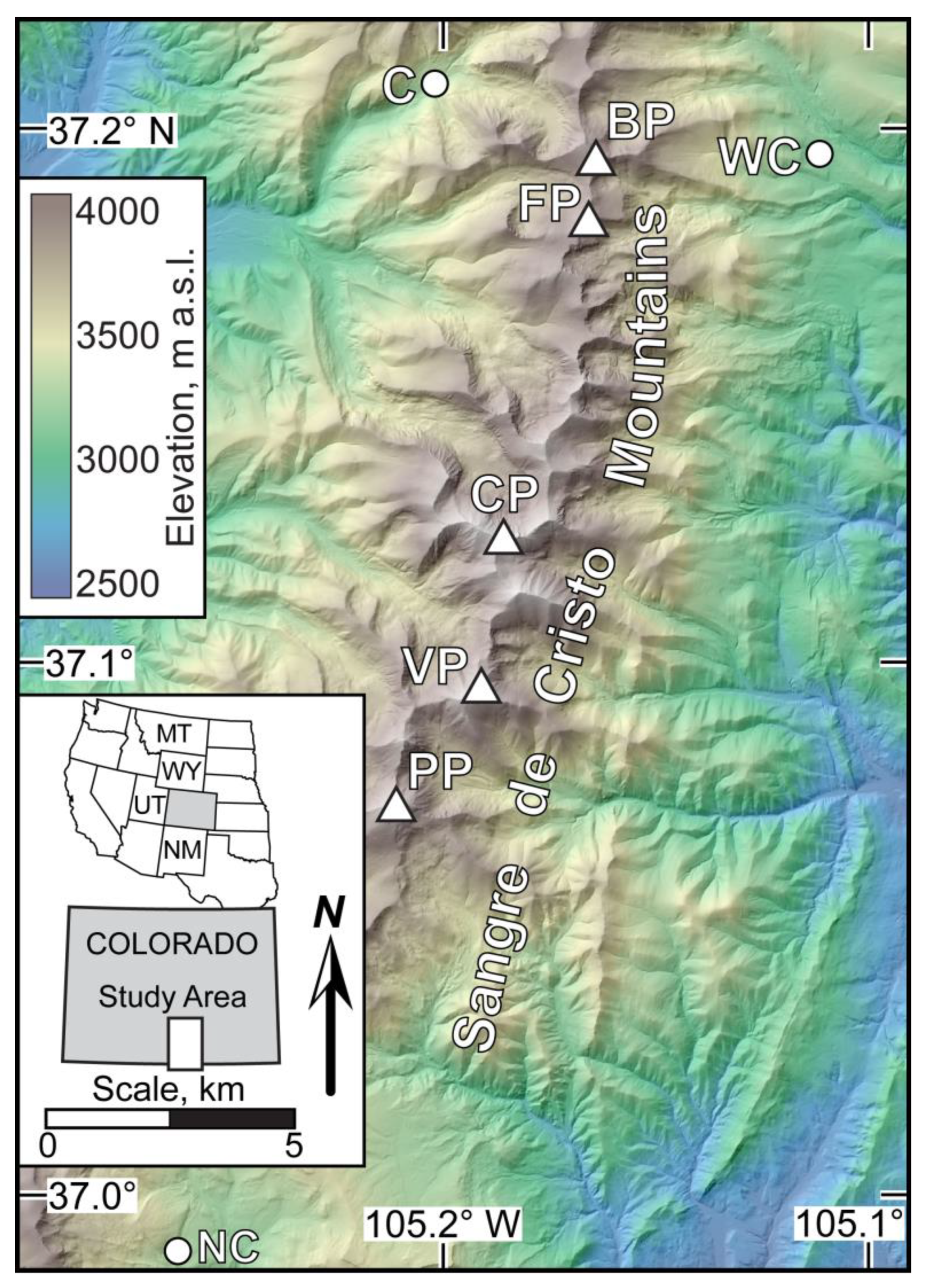
Figure 1. Location map of the study area in the Sangre de Cristo Mountains of Colorado. Abbreviations in inset map: MT—Montana; NM—New Mexico; UT—Utah; and WY—Wyoming. Circles are SNOTEL stations used to define modern climate and test model skill. Triangles are several of the prominent peaks in the region. Abbreviations: C—Culebra SNOTEL; NC—North Costilla SNOTEL; WC—Whiskey Creek SNOTEL; BP –Beaubien Peak (4016 m); CP—Culebra Peak (4280 m); FP—Francisco Peak (3999 m); PP—Purgatoire Peak (4169 m); and VP—Vermejo Peak (4168 m). Shaded relief image is from the United States Geological Survey 3D Elevation Program 1 m Digital Elevation Model via OpenTopography. https://doi.org/10.5069/G9NP22NT (accessed on 21 July 2025).
Quaternary 08 00064 g001
Figure 2. Median temperatures and precipitation recorded at SNOTEL stations for 1990–2020 normals. Temperatures from individual stations are small (~1–2 °C) and therefore standard deviations are omitted for clarity, whereas standard deviations for precipitation as shown are significant.
Quaternary 08 00064 g002
Figure 3. Reconstructed paleoglaciers in the study area at their LGM extents. Glaciers and/or ice masses not reconstructed are shown schematically, and not all are shown here. Abbreviations as in Figure 1.
Quaternary 08 00064 g003
Figure 4. Comparison of modeled and observed 1991–2020 median (a) temperatures and (b) precipitation at SNOTEL stations. NSE are the Nash–Sutcliffe Efficiency statistics, and ∑abl and ∑acc are the cumulative differences for the ablation and accumulation seasons (shaded), respectively (see text for discussion). (c) Modeled and observed snowpack evolution at the SNOTEL stations.
Quaternary 08 00064 g004
Figure 5. (a) Steady-state ELAs of the paleoglaciers and associated LGM temperature depressions based on temperature-index modeling. Results for western and eastern slopes are shown in red and blue respectively. Bold lines in the shaded boxes are the mean values and the shading reflects the standard deviation. Error bars in individual values of temperature depression reflect different melt factor scenarios (see text for discussion). (b) Comparison of modeled and AAR-derived ELAs. Color and shading as in (a). Abbreviations and numbering: 1, SV—South Vallejos; 2, NV—North Vallejos; 3, BC—Bernardino–Carneros; 4, EP—El Perdido; 5, WK—Wilkens; 6, ALF—Abbot–Left Fork Abbot; and 7, LV—Las Vigas. Diagonal line represents concordance between ELAs. (c) Average temperature depressions required for steady-state mass balance assuming different combinations of LGM precipitation and melt factors used in the modeling.
Quaternary 08 00064 g005
Figure 7. CHELSA-TraCE21k downscaling of LGM changes in LGM precipitation (a,b) and temperature (c,d) with respect to modern. The geographic extent of (a,c) is the same as that shown in Figure 6. The study area is shown in (b,d). White triangles indicate major peaks with abbreviations as in Figure 1. The red and white outlines in (b,d) delineate the extent of the reconstructed glaciers; nunatacks and unglaciated interfluves are not shown. Note color scales are different in each panel.
Quaternary 08 00064 g007
Table 1. Surface area, length, mean and maximum thickness, driving stresses, and AAR-derived ELAs of reconstructed glaciers.
GlacierAreaLength, km *Average IceMaximum IceDriving Stresses,AAR-Derived ELA, m †
km2kmThickness, m *,†Thickness, m *,†kPa ** (Mean)=0.65=0.70=0.60
Western slope
South Vallejos7.025.810513053–118 (93)347034403500
North Vallejos7.957.610515573–156 (95)348534353525
Bernardino-14.237.510515083–131 (113)341533653465
Carneros †† 7.311016065–122 (91)
El Perdido3.254.67510055–152 (90)355035253580
Means348034403520
Eastern slope
Wilkens4.656.110513066–135 (108)333032853370
Abbot-Left6.877.0608050–154 (95)334532903400
Fork Abbot †† 5.16010052–187 (98)
Las Vigas3.095.9709552–144 (98)338033203430
Means335533053405
* Longest flow line where applicable. † Nearest 5 m, likely minimum estimates owing to till and post-glacial fluvial deposition. ** Calculated at a number of ice contours. †† Although likely confluent, treated here as individual glaciers except glacier area and ELAs. Named first valley is larger area and length of subordinate glacier is that to the confluence.
Table 2. Comparison of modeled modern temperatures (°C) during the ablation season and precipitation (mm) during the accumulation season with PRISM values at given elevations (m) in pertinent regions. denotes cumulative values during the respective seasons. Positive differences in temperature reflect cooler modeled temperatures, those in precipitation indicate drier conditions. Differences in precipitation are also given in percent (rounded). NSE is the Nash–Sutcliffe Efficiency statistic. Mean difference uses the absolute values.
Elevation (n) *TablationNSEablationPaccumulationNSEaccumulation
North and South Vallejos Valleys
3999 (3)−0.60.98+23 (+4%)0.93
3801 (5)+0.10.98−11 (−2%)0.97
3601 (5)+0.20.98−12 (−3%)0.97
3398 (4)+0.80.98+1 (<1%)0.99
3195 (6)−0.20.97+7 (+2%)0.97
3001 (6)−0.60.99−11 (−3%)0.92
Means0.4 9 (2%)
Bernardino, Carneros, and El Perdido Valleys
3900 (3)−0.60.98+22 (+4%)0.95
3750 (8)+0.050.98+7 (+1%)0.99
3599 (3)+0.60.98−50 (−10%)0.70
3450 (5)+0.60.98−25 (−6%)0.91
3198 (4)−0.60.98−1 (0%)1.00
Means0.5 21 (4%)
Wilkens Valley
3865 (3)−0.20.99+31 (+5%)0.91
3654 (4)−0.60.98+25 (+5%)0.91
3291 (3)+1.00.98+5 (+1%)1.00
3054 (3)−0.20.98+2 (<1%)0.85
Means0.5 16 (3%)
Abbot, Left Fork Abbot, and Las Vigas Valleys
3904 (4)+0.70.98−6 (−1%)0.93
3771 (4)−0.10.98+29 (+5%)0.85
3497 (6)+0.40.98+39 (+9%)0.84
3299 (3)+0.40.98+18 (+4%)0.94
2994 (6)−0.20.99−20 (−6%)0.72
Means0.4 22 (5%)
* Elevations represent mean values of n—number of PRISM grid points “clustered” around target elevations (generally ± ~25 m or less). Note elevations, elevation range, and n are constrained by PRISM data in each region.
Table 3. Temperature depressions (∆T) with or without accompanying annual precipitation changes (∆P) required to maintain steady-state mass balances of reconstructed paleoglaciers and steady-state ELAs. Average melt uses mƒ for snow and ice equal to 7.0 and 4.5 mm w.e. °C−1 d−1, reduced melt uses 5.0 and 2.5 mm w.e. °C−1 d−1, and for enhanced melt 9.0 and 6.5 mm w.e. °C−1 d−1.
Glacier∆T (°C; ∆P = 0)∆P (mm) *ELA †
Average MeltReduced MeltEnhanced Melt+200+100−100−200
   West slope
1. South Vallejo9.48.79.79.09.29.59.73485
2. North Vallejo9.48.79.89.09.29.69.83475
3. Bernardino-Carneros9.79.010.19.39.59.910.23435
4. El Perdido8.78.19.18.48.58.99.13565
   Means9.38.69.78.99.19.59.73490
   East Slope
5. Wilkens9.89.110.39.59.710.010.33385
6. Abbot-Left
  Fork Abbot10.29.510.79.910.010.510.73325
7. Las Vigas9.58.810.09.19.39.810.03425
   Means9.89.110.39.59.710.110.33380
   Grand means9.58.810.09.29.39.710.03440
   Reduced melt, means 8.48.69.19.3
   Enhanced melt, means 9.69.810.110.3
* Average melt factors. † ELA is for average melt and no change in precipitation and rounded to nearest 5 m.
Disclaimer/Publisher’s Note: The statements, opinions and data contained in all publications are solely those of the individual author(s) and contributor(s) and not of MDPI and/or the editor(s). MDPI and/or the editor(s) disclaim responsibility for any injury to people or property resulting from any ideas, methods, instructions or products referred to in the content.