Revisit the Medieval Warm Period and Little Ice Age in Proxy Records from Zemu Glacier Sediments, Eastern Himalaya: Vegetation and Climate Reconstruction

Abstract

The Late Holocene fossil pollen records from the Zemu glacier, located in Yabuk, North Sikkim, in the eastern Himalayas, effectively generated quantitative climate reconstructions based on the transfer function model. The transfer function model was developed by establishing a modern pollen–climate calibration set from the temperate alpine belt of North Sikkim. A redundancy analysis was carried out to detect the pattern of variation of climatic variables in the modern pollen datasets. The mean annual precipitation (MAP) and mean temperature of the warming month (MTWA) had the strongest influence on the composition of the modern pollen samples among the climatic variables considered in the analysis. Proxy data in the form of fossil pollen records were analyzed for reconstructing past climate based upon the relationships between modern pollen vegetation assemblages and climatic patterns. Transfer functions for MAP and MTWA were developed with the partial least squares (PLS) approach, and model performance was assessed using leave-one-out cross-validation. The validated model was used to reconstruct MAP and MTWA for the last 2992 cal years BP (1042 BC) in North Sikkim. The variability observed in the reconstructions was analyzed for past global climatic events. It was further compared with the available regional and hemispheric proxy-based climate reconstructions. The reconstructions captured comparable Medieval Warm Period (MWP) and Little Ice Age (LIA)-like events from the Zemu glacier region. The fossil pollen data and climate reconstructions were further compared with the mineral magnetism data of the subsurface sediment profile.

1. Introduction

The decadal-to-millennial-scale climate variability records of the Quaternary period are of significant interest to scientists; their chronology and mechanisms have been widely discussed, prompting extensive analysis and recommendations [1]. However, further detailed analysis is needed in order to obtain a deeper understanding of the authenticity of past climate change studies. An introspective look at the dynamics and functioning of the past climatic system will allow us to understand its behavior and patterns in the future. This will improve greatly if long-term climate data are available beyond the existing instrumental records. Thus, palaeoclimatic data are essential to obtain comprehensive information about the past climate system, without which reliable forecasting of future conditions will not be possible [2]. High-elevation mountainous regions also represent unique areas for the detection of climatic change and the assessment of climate-related impacts [3]. One reason for this is that, as the climate changes rapidly with altitude over relatively short horizontal distances, so do vegetation and hydrology [4]. Past climate records from such high-elevation mountainous regions and remote areas can be used to evaluate the regional climate and its association with global climate dynamics. These high-altitude environments comprise glaciers, snow, permafrost, water, and the uppermost limits of vegetation and other complex life forms in the mountains, and they are the most sensitive to climatic changes occurring on a global scale [5].

Instrumental meteorological records from high-altitude sectors of the Himalayas, such as regions in proximity to glaciers, do not cover a longer time span as they were not recorded before the last century. Thus, assessing long-term climatic variability in higher elevations and remote regions of the Himalayas as well as its future impact is hindered by the paucity of long-term meteorological and glaciological observations. For this, extensive climate records from natural archives and proxies are required. Based on these natural archives or proxy data, detailed climate reconstructions have been carried out globally [6,7]. Proxy-based climate reconstructions can be useful to place recent climate trends in the context of a longer time scale. These climate reconstructions allow a comparison to be made of recent trends with past climatic variation and with well-known climatic events of the Late Holocene period, such as the Medieval Warm Period (MWA), or Epoch (MWE) [8], more recently coined as the Medieval Climatic Anomaly (MCA) [9,10,11], and the Little Ice Age (LIA) [12]. It also facilitates assessing the local pattern of climate variability in a regional, continental, hemispheric, and global context. The quantitative climate reconstructions from the Himalaya region are mostly available from tree-ring proxy records [13] and are highly concentrated in the western Himalayan region [13]. Only a few tree-ring-based temperature reconstructions are available from the eastern Himalayas, including parts of India [14,15] and Bhutan [16]. Tree-ring data were used by Bhattacharyya and Chaudhary [14] for temperature reconstruction from the eastern Himalayan region carried out in sites close to the present pollen study sites.

The pollen grains preserved in sub-surface sediments have been extensively studied as a proxy indicator of palaeoclimatic and palaeoecological changes during the Quaternary period [7,17], and many methodological advances in various fields have been made during the last five decades [18,19,20,21,22]. Palynological analysis of the Quaternary sediment from temperate to alpine regions of the Himalayas has been carried out for past vegetation vis-à-vis climate analysis [23,24]. These records mainly show qualitative past climate based on the vegetation assemblages during the Late Quaternary. However, quantitative past climate reconstruction using the pollen dataset is poorly studied in the Indian Himalayan region and absent from Sikkim in the eastern Himalayas [25]. In spite of the fact that quantitative climate reconstruction of temperature and precipitation based on modern pollen–climate relationships are useful for perceiving Quaternary Palaeoecology and Palaeoclimatology [26], various climatic variables such as mean annual temperature (MAT), mean temperature of the coldest month (MTCO), mean temperature of the warmest month (MTWA), and mean annual precipitation (MAP) are widely experimented climatic parameters. These have been applied in several quantitative climatic reconstructions using a variety of proxies. After the pioneering works of Iverson [27] and Grichuk [28], pollen data from lacustrine and sedimentary archives became the most frequently used proxy to quantify changes in the Holocene and Pleistocene climate from various geographical regions [29]. The algorithm for the reconstruction of environmental variables using biological proxies was introduced long ago by Imbrie and Kipp [30]. Since then, pollen climate transfer functions have been widely attempted for the quantitative reconstruction of climatic parameters on different geological time scales from various parts of the globe [31,32,33,34,35,36,37,38,39,40,41,42,43,44,45,46,47,48,49,50,51,52]. Pollen-based quantitative climate reconstruction has made great strides over the past few decades in various parts of the world, using several different reconstruction techniques [53]. Transfer function-based climate reconstruction using pollen records has also made advances in Asian subcontinents [54,55,56,57,58,59,60,61,62,63,64,65,66].

The strengths and weaknesses of quantitative climate reconstruction using pollen as a proxy, modeled with discrete transfer function methods as demonstrated in the reviews [17,20,26,37,38,67,68,69,70,71,72,73,74,75,76], are discussed by Birks [77]. However, these widely studied climate reconstruction techniques have not been widely applied in the eastern Himalayan region despite the availability of the pollen-based Late Quaternary records [25]. There are few studies in which the coexistence approach has been used to reconstruct quantitative climate during the Late Quaternary period using pollen [78] and phytolith [79] records from the eastern Himalayas. The coexistence approach was introduced by Mosbrugger and Utescher [80] for the quantitative reconstruction of Tertiary terrestrial palaeoclimates using plant fossils. It is not widely used for fossil pollen-based climate reconstruction, especially for the Holocene. The limited take-up of the coexistence approach in Holocene studies is because other related methods, such as direct transfer functions, are available [81]. However, this technique has been used in China for several Holocene pollen records [82,83].

The fossil pollen studies previously carried out in Sikkim have mostly deduced past vegetation with qualitative reconstructions of the climate. Late Holocene vegetation climate history was reported based on fossil records from Khechipiri Lake [84] and Kupup Lake [85] located in Sikkim, the Himalayas. In the adjoining temperate parts of this region, few fossils pollen studies have been carried out [86,87]. Sharma and Chauhan [86] have reported vegetation history dating from the Last Glacial Maximum (LGM) based on pollen records from Mirik Lake, Darjeeling Himalaya. Other studies from Jore-Pokhari, a temperate lake located in Darjeeling Himalaya [87], described qualitative climatic records since 2500 cal. BP. In addition, there is no modern pollen climate calibration set that is a pre-requisite for quantitative climate reconstruction. The surface pollen spectra from Sikkim Himalaya have been studied at only one site [85]. The study included the relationship between vegetation and modern pollen rain from the Kupup Lake vicinity using 12 surface samples, but no quantitative comparisons with the modern climate of the region have yet been established. Similarly, there is one recent study of only modern pollen data sets from the North Sikkim region, and emphases have been placed on the feasibility of the data for future palaeovegetation and palaeoclimatic reconstruction [88]. However, in this study, no pollen fossil data sets were utilized for palaeoclimate reconstruction. Thus, the development of pollen-based quantitative climate reconstruction using the transfer function model in the eastern Himalayas is needed.

Here, we make the first attempt to reconstruct climate in quantitative terms and to assess its past variation at the Zemu glacier, eastern Himalaya. We try to establish the possible roles of regional climate, global teleconnection, and long-term climate variation in the Zemu glacier, eastern Himalaya. In this study, modern pollen climate calibration was established and applied to a Late Holocene fossil pollen record from Yabuk, Zemu glacier, North Sikkim, for quantitative past climate reconstruction. The reconstructed climatic variables were further compared to the environmental geomagnetic data of the profile sediments. The study of the mineral magnetic properties of sediments has become an increasingly useful tool to understand the input of sediment flux in different depositional environments containing iron mineral particles [89,90,91,92,93]. The technique is useful for reconstructing climate and environment because the mineral magnetic characteristics of sediments are sensitive to variations in climate, transport medium, and environmental conditions [90,91,94,95,96]. Lake sediment properties of magnetic susceptibility and remanence reflect past limnological conditions and have been widely used as climate proxies in high-altitude Himalayan palaeolake sediments [97,98,99,100,101].

The measured environmental magnetic parameters are also sensitive to magnetic grain size variations, and, subsequently, the determination of environmental changes at the site and depositional environments [89,90,91]. The magnetic grain size and thus domain structure of iron minerals in sediments range between multidomain (MD), stable single domain (SSD or SD), pseudo-SD (PSD), and superparamagnetic (SP) grains. Information about the magnetic grain size in sediments can be used to identify sediment provenance areas [102,103]. We describe here the magnetic mineral data with reference to the pollen zone constituting the sediment profile. This has been carried out to identify the similarities and significance of the magnetic data and the palynological interpretations.

Inferences were further drawn to highlight the changes occurring in the Late Holocene climate at the Zemu glacier, North Sikkim, and their regional and global teleconnections to other existing proxy-based qualitative and quantitative records.

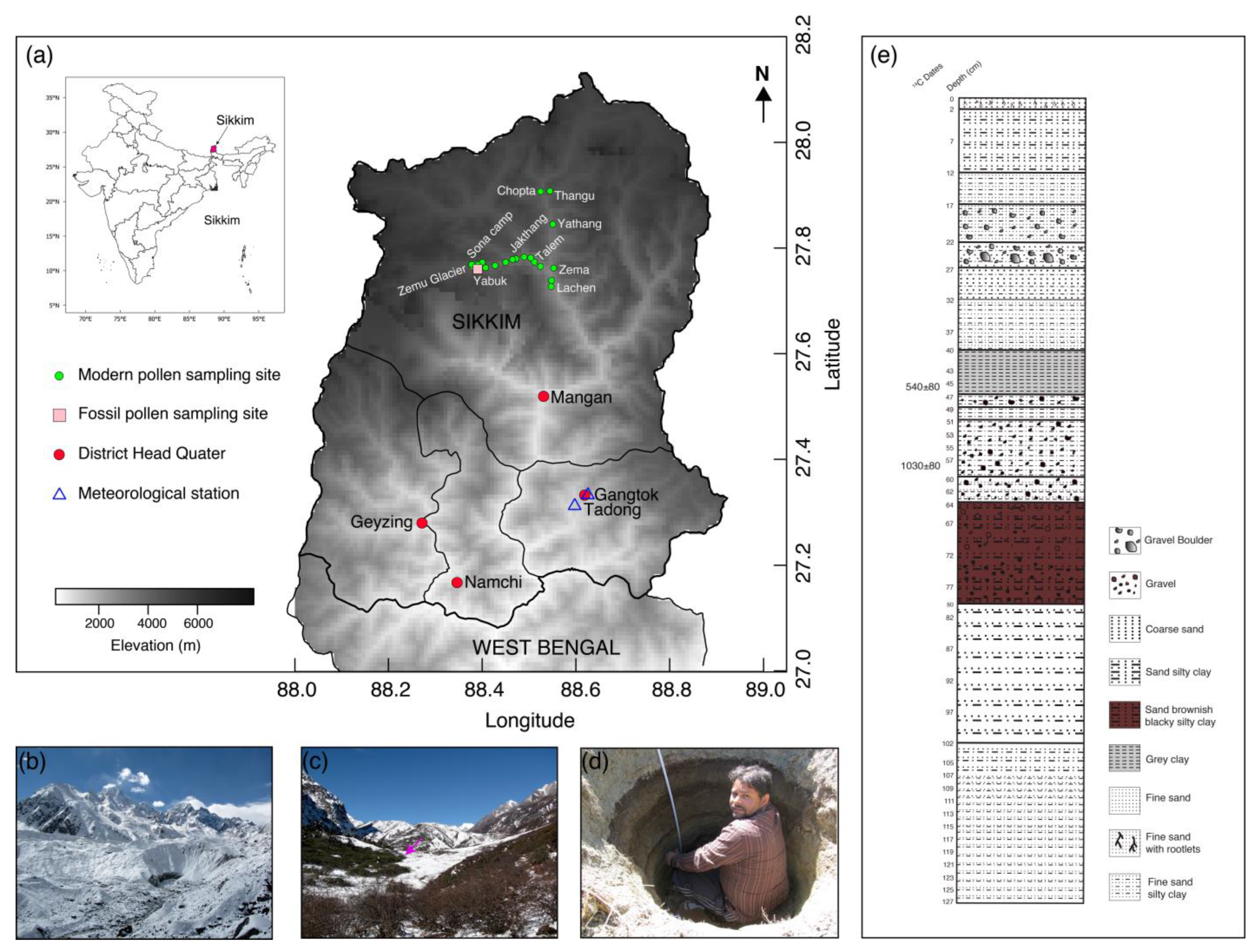
2. Materials and Methods

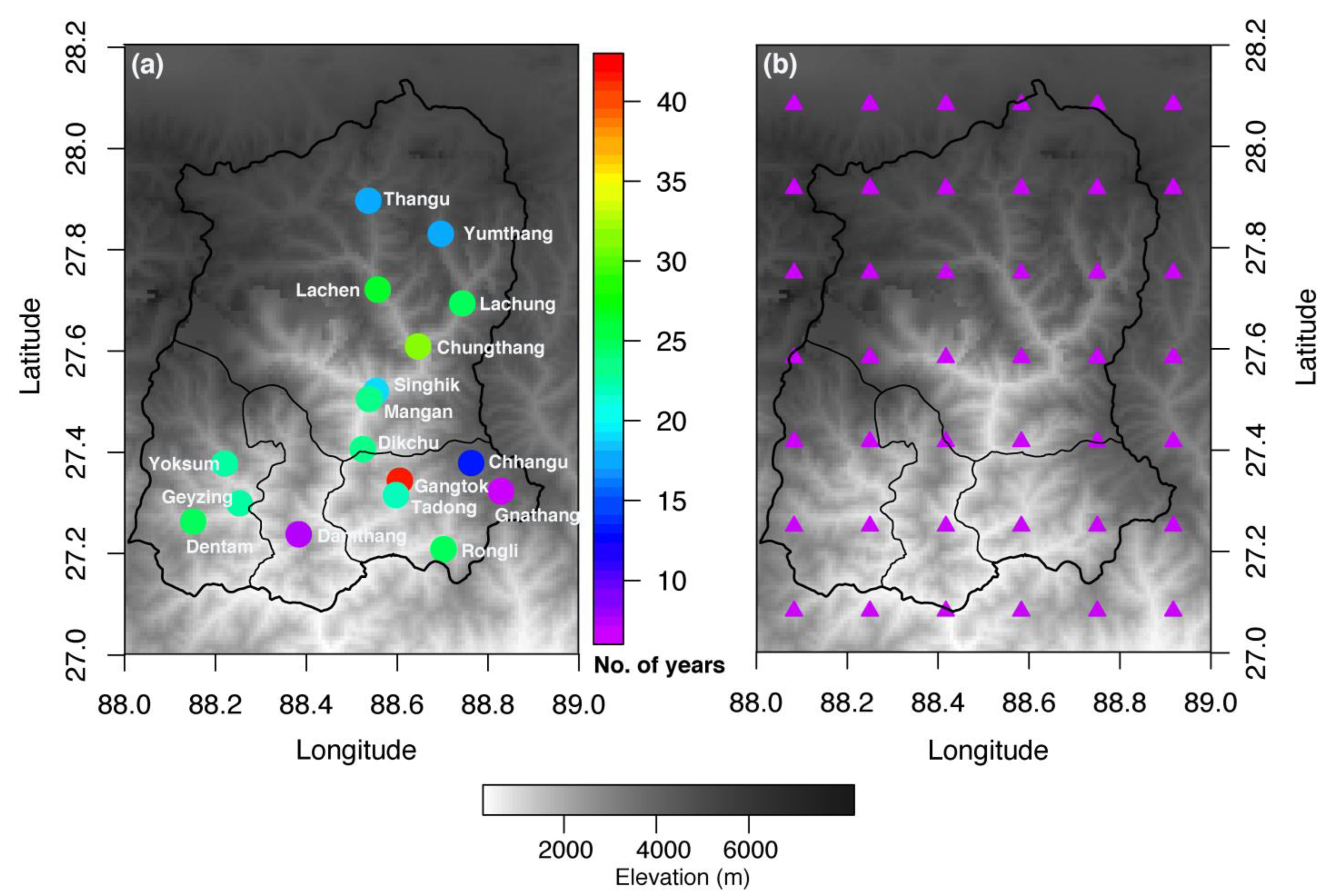
Study Sites, Environmental Setting and Vegetation

The Sikkim Himalayas are occupied by glacierized basins, mostly in the western and northern regions of the state. Most of these glaciers drain their water into the Tista River and are commonly termed Tista Basin glaciers. The four main glacier basins are the East Rathong basin, Talung basin, Changme Khangpu basin, and Zemu basin, covering about 7172.21 km². Among these, the Zemu Basin occupies an area of 2391.60 km², covered by 250 glaciers. This basin contributes to two major tributaries, the Zema Chhu (‘Chhu’: river) and Hema Chhu [104]. The Zemu Chhu is the main feeder of the river Tista. The present study site is situated in the Zemu glacier basin, North Sikkim (Figure 1), which is part of the eastern Himalaya region. The Zemu glacier lies on the eastern face of Kanchendzonga peak and is the largest (41.2 km²) and longest (28 km) glacier in the Sikkim Himalaya region [105]. The Zemu glacier originates from the eastern flank of the Kanchendzonga ridge. The glacier flows in an easterly direction, draining towards the northern slopes of Simvo and Sinialchu. The glacier has many trenches on its northern and southern sides between the lateral moraine ridges and the rock wall [106]. These trenches have arisen due to the lateral shrinkage of the glacier [106,107]. The Zemu glacier region is situated towards the north of the Main Central Thrust (MCT) and is composed of Kanchenjunga Augen-Gneiss. The porphyritic augen-gneisses with streaks of biotite are recorded towards the north of Lachen [108]. Bands of calc-gneisses stratified along with the augen-gneiss exist near the Zemu-Lachen confluence. In the northern region of Sikkim, there are many granitic masses and aplitic veins found from Chungthang in the Tista valley to Jakthang in the Zemu valley. There are also granite and pegmatite veins ranging from 1 cm to 1 km in thickness between Chungthang and Lachen [104].

Sikkim is influenced by monsoon winds originating from the Bay of Bengal. The Bay of Bengal lies towards the south of the Sikkim Himalaya and brings more rainfall to the region from May to October. The high elevations are also under the influence of the Tibetan Plateau, which plays an important role in generating the Asian monsoon and influences the atmospheric circulation due to the freezing and thawing of the plateau [109,110]. The topographical variations along the Teesta valley give rise to a mostly humid climate within the mountainous walls of the region [111]. Apart from two meteorological stations, Gangtok and Tadong, where fully-fledged meteorological observatories have been functioning since 1957 and 1978, respectively, other stations are mainly rain gauge stations, and records are available from approximately 4 to 25 years ago [111] (Figure 2). The majority of the state receives heavy rainfall throughout the year, while the months of October–March remain comparatively drier. The mean annual rainfall is minimum (82 mm) at Thangu, North Sikkim, and maximum (3494 mm) at Gangtok. Places with an altitude of 6065 m and above are snowbound, and places as low as 3002 m come within the snowline in the winter. The temperature in the lower altitudes fluctuates between 4 °C and 35 °C, and the temperature of places with moderate altitudes (around 1829 m), such as Gangtok, varies between 1 °C and 25 °C. In high-altitude areas (above 3993 m), the temperature never rises above 15 °C and slides down to freezing point in winter [104].

The vegetation of Sikkim has three discrete botanical zones: tropical, temperate and alpine, distributed according to the elevation and characteristics of the vegetation [112]. The vegetation of the state is classified as low, middle, and upper hill forests, followed by rhododendron-conifer zones and Alpine scrubs and grassland [112]. The present study area falls under Rhododendron-conifer (cold temperate or sub-alpine zone, 2700–3600 m) and alpine scrub and grasslands (3600–4300 m and above). The dominant tree taxa along the sampling sites are mostly conifers: Abies densa, Juniperus recurva, Larix griffithiana, J. squamata, Picea spinulosa, and Tsuga dumosa, and broad–leaved taxa: Betula utilis and Rhododendron spp. At the termination of the tree line above 3600 m, J. pseudosabina and J. recurva grow as scrubs on hill slopes. The stunted height of Rhododendron spp was observed growing on exposed rock crevices at altitudes of 3600 m or above. Ephedra gerardiana were found growing only on the hilltops around Thangu. A few species belonging to genera such as Ranunculus, Anemone, Delphinium, Rhus, Potentilla, Primula, Fragaria, Cassiope and Allium were seen on the gentle slopes of open meadows. The detailed vegetation of Zemu Valley in Sikkim Himalaya has been thoroughly enumerated by Smith and Cave [113].

The detailed methodology for the present study has been described in the Supplementary Information for surface and sub-surface sediment sampling, pollen analysis [114,115,116] of modern and fossil pollen, mineral magnetism analysis [89,90,91], chronology, and age-depth model [117], modern climate [111,118,119,120], numerical analysis [38,70,72,73,76,77,121,122,123], and palaeoclimatic reconstruction [124,125,126,127,128,129,130,131]. We further describe the results obtained from these particular analyses of the samples collected from Zemu glacier region and its surroundings.

3. Results

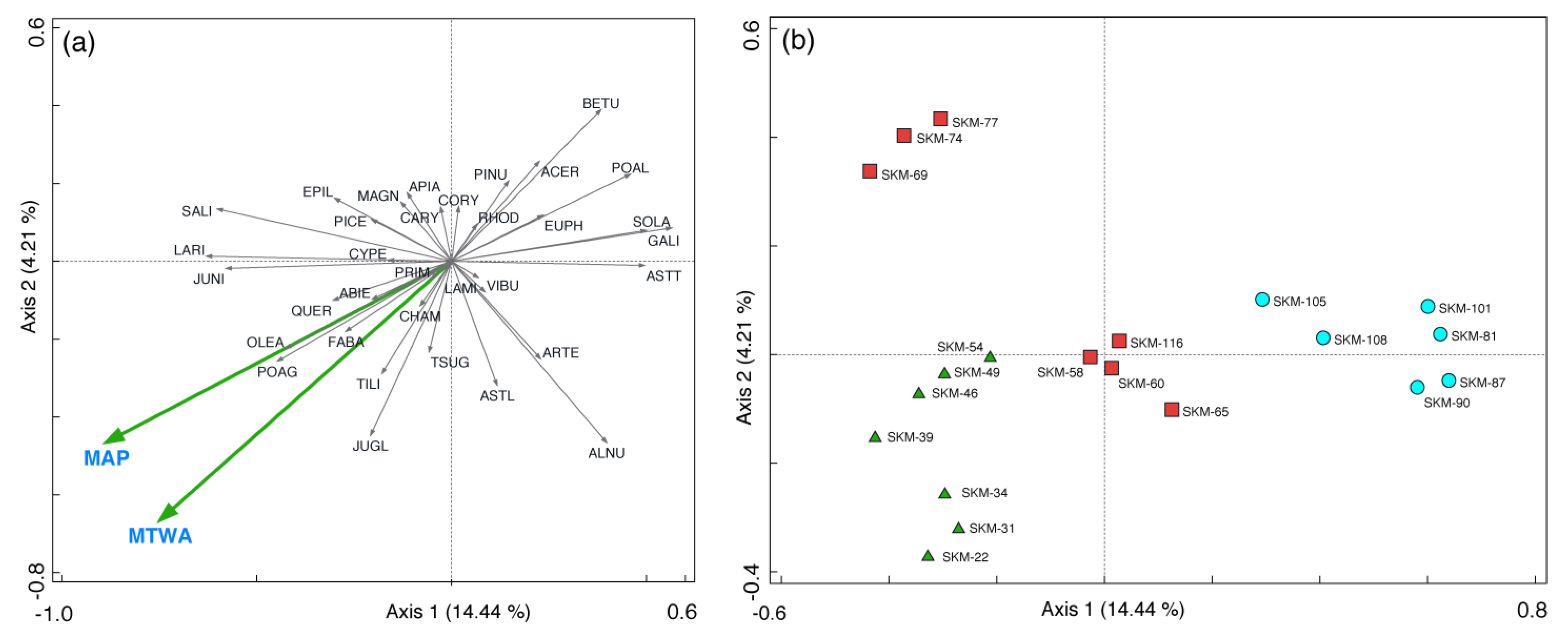
3.1. Modern Pollen Sites and Assemblages

The modern pollen sampling sites considered in the present study are well represented in the north-west transect (Lachen to Zemu Glacier) but the densities are relatively low in the northern transect of Lachen towards Thangu (Figure 1). These sites cover vegetation zones ranging from sub-tropical to temperate to alpine, with both coniferous and broad-leaved elements. The climatic variation of these sites ranges with gradients in MAT (1.4–10.6 °C), MTCO (−7.4–2.6 °C), MTWA (9–16 °C), MAP (61–145.5 mm), and elevation (2600–4311 m) based on gridded climate data sets (Figure 3). The details of the gridded climate data have been described in Supplementary Information.

3.2. Ordination

The unconstrained ordination using PCA showed that the first two axes capture 49.1% (axis 1, 31.1%; axis 2, 18.0%) of the total variance. This suggests that only a few variables dominate the data structure, but they are considered high in such high-elevation and climatically contrasting regions. The constrained ordination using RDA with pollen and climate data (MAP and MTWA) showed the eigen values of the first and second axes are 0.1444 and 0.0421, explaining 77.43% of the total variance in the pollen assemblage data (Figure 4 and Figure 5). The RDA was also carried out with MAP and MTWA separately. The first RDA axis captures 12.23% variance in the pollen datasets and shows significant correlation with MAP (r = 0.696, p < 0.02), while with MTWA, the first axis captures 9.93% variance with significant correlation (r = 0.667, p < 0.046). The RDA with MAP and MTWA variables shows a similar pattern to the PCA, suggesting that both the variables have a strong influence on the underlying structure of the modern pollen data.

In RDA, some pollen taxa are grouped together and some are separated (Figure 5). The RDA axis 1 segregated coniferous taxa (Juniper, Larix, Abies, Picea and Tsuga) and broadleaved taxa (Juglandaceae, Quercus, Salix, Fabaceae and Oleaceae) on the left side. The coniferous taxa (Pinus) and broadleaved taxa (Betula, Alnus, Acer, Corylus, Rhododendron and Magnoliaceae) were separated on the right side of axis 1. It was shown that apart from Pinus, all other conifer taxa were grouped together by axis 1. The RDA axis 1 also differentiated in the pollen assemblage of wild grass (Poaceae < 50 µ) and cultivated grass (Poaceae > 50 µ) on two sides of the axis. Most of the shrub and herb elements were concentrated in the center of the ordination and did not show clear segregations.

The modern pollen sites were separated in RDA according to climatic influence (Figure 5). The first RDA axis segregates sites with MAP (60.9–79.0 mm) and MTWA (9.0–10.3 °C) from sites with MAP (116.5–145.5 mm) and MTWA (13.2–16.4 °C). The sites separated by RDA axis 1 are comparable with the altitudinal gradient. The sites (SKM081, SKM087, SKM090, SKM101, SKM105 and SKM0108) segregated on the right side of axis 1 (Figure 5) have low MAP and MTWA, are from a higher elevation (4016–4311 m), and are mostly closer to the Zemu glacier and within its vicinity, which is in an alpine climate. The sites (SKM022, SKM031, SKM034, SKM039, SKM046, SKM049 and SKM054) with high MAP and MTWA segregated on the left side of axis 1 (Figure 5) are mostly from a lower elevation (2600–3303 m) and are influenced by a cool, temperate climate. The sites (SKM058, SKM060, SKM065 and SKM116), which are laid in intermediate and close to the center of both axes, and sites (SKM069, SKM074, SKM077), isolated on the left side of axis 1, are mostly influenced by both the higher and lower elevation climatic conditions of the region, with moderate MAP (95.9–109.7 mm) and MTWA (10.5–12.5 °C). The altitudinal gradient of these sites ranges from 3501 to 3915 m, with a sub-alpine climate, and seems segregated under the influence of RDA axis 2 (Figure 5). Similar segregation was observed when the modern pollen data were grouped in zonation (Figure 4) using unconstrained chord-distance clustering (CONISS) on a square-root-transformed modern pollen percentage assemblage.

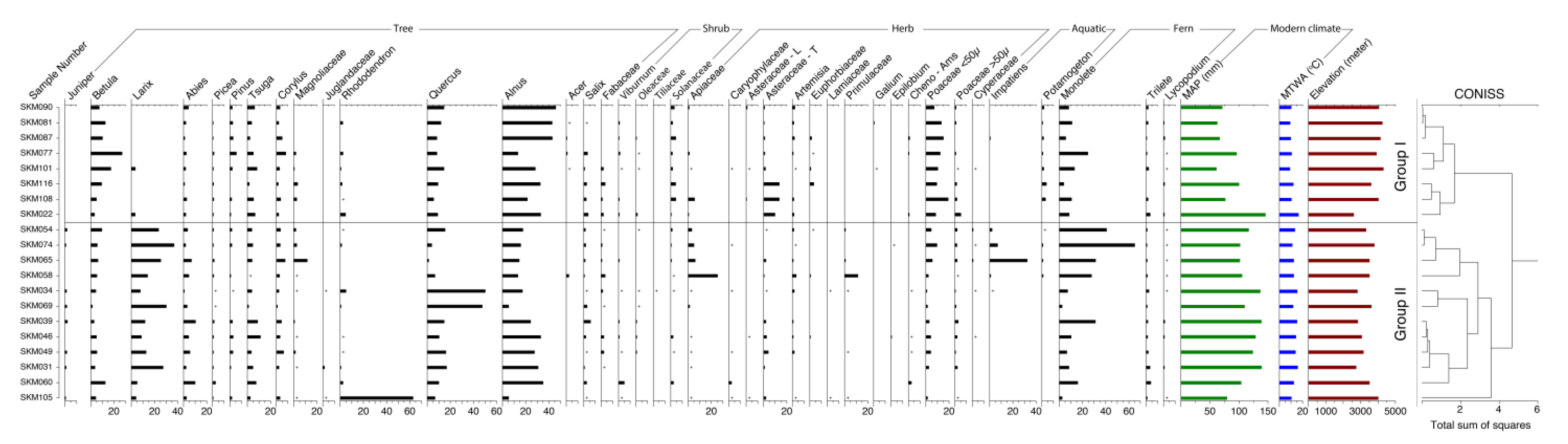
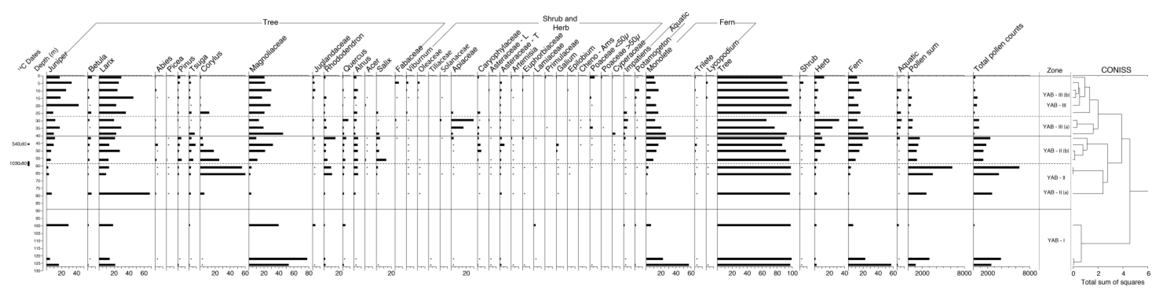
3.3. Chronology and Palaeo–Vegetation History

Based on the derived chronology using linear regression, the Yabuk sediment profile covers the last 2992 cal years BP (1042 BC), confirming that these sediments belong to the Late Holocene. So, the present fossil records represent the vegetation and climate records since the Late Holocene. The chronology detail of the fossil sediment profile is provided in

Table 1. Radiocarbon ages and calibration.

	YABUK 12	YABUK 18
Depth (cm)	46	58.5
14C Radiocarbon age	540 ± 80	1030 ± 80
Calibrated age (cal yrs BP)	566	945
Calendar age (BC/AD)	1384	1005

. The rate of sedimentation calculated was mostly similar from top to bottom in depth, and its average rate was 0.08 cm/year.

Based on the CONISS of the percentage of pollen data, three zones, YAB–I, YAB–II and YAB–III, were established to represent the major phase of vegetation change. Two zones, YAB–II and YAB–III, are further divided into two sub-zones to represent the minor vegetation changes within the broad phase (Figure 6). The vegetation changes in each zone are described in Supplementary Information.

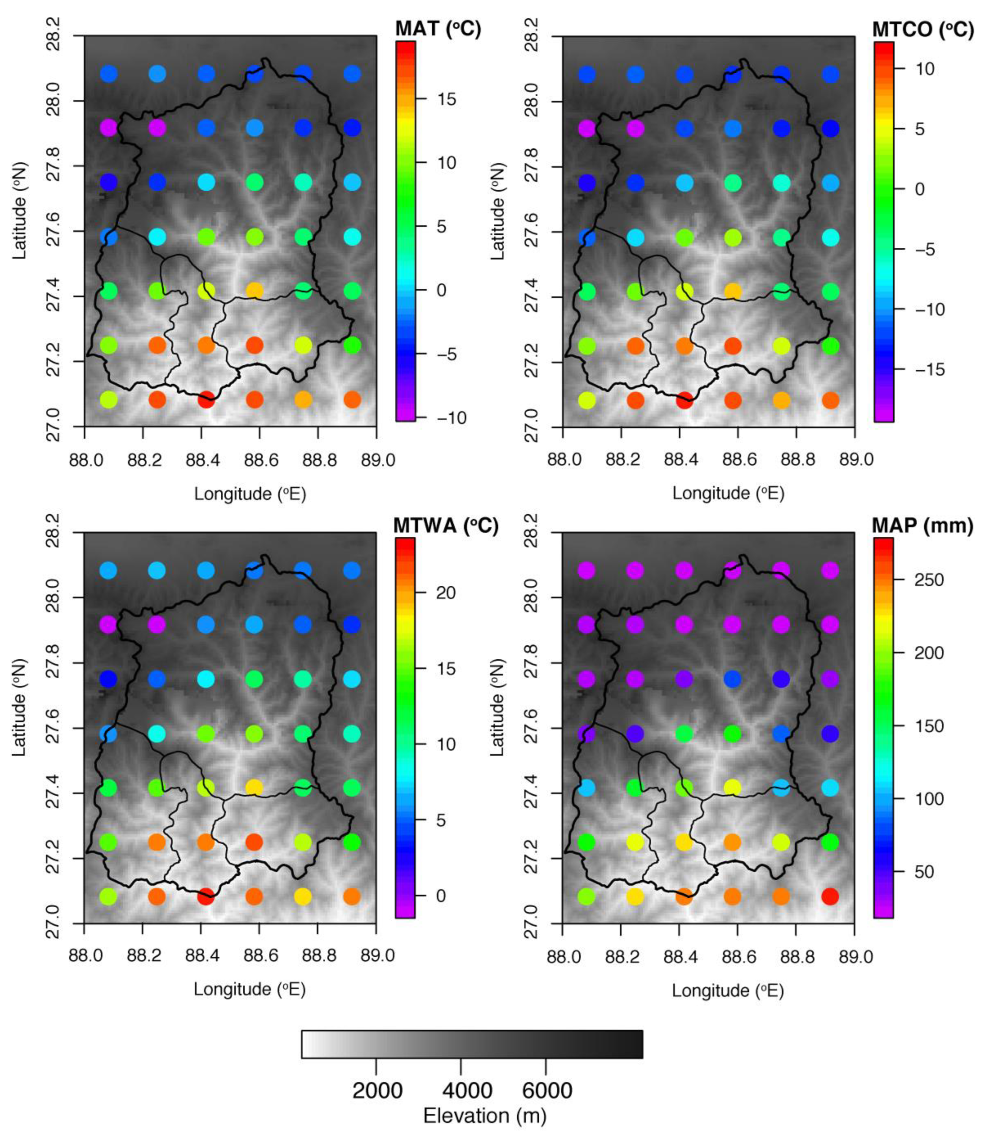
3.4. Pollen–Climate Calibration and Transfer Function

The RDA shows that there is a statistically significant relationship between modern pollen assemblages and the climatic variables MAP and MTWA (Figure 5). A transfer function was developed for MAP and MTWA as these were the significant climatic variables entered in the ordination analysis, RDA. Prior to final model development, we found four samples (SKM022, SKM069, SKM074 and SKM101) producing extreme values in the analyses. These sites were removed from the training set prior to performing PLS regression and calibration. The improved pollen-climate PLS transfer function was finally developed based on the screened dataset (

Table 2. Model performance statistics as assessed by leave-one-out cross-validation for the using first x (x = 1–6) components of the partial least square regression (PLS). Component marked with * are used for further analysis and for climate (MAP and MTWA) reconstruction.

	Apparent		Cross-Validated (Leave-One-Out)
PLS Component	RMSE	Correlation (r2)	RMSEP	Correlation (r2)
MAP
Component 1 a	19.017	0.479	23.593	0.235
Component 2 a	14.034	0.717	25.818	0.207
Component 3 a	11.679	0.804	27.380	0.213
Component 4 a	9.412	0.873	33.026	0.129
Component 5 a	7.650	0.916	36.318	0.116
Component 6 a	6.674	0.936	38.949	0.105
Component 1 b	13.061	0.734	18.501	0.473
Component 2 b	8.783	0.880	18.918	0.480
Component 3 b	5.574	0.952	18.699	0.505
Component 4 b	4.062	0.974	18.688	0.514
Component 5 b	3.558	0.980	17.103	0.580
Component 6 b *	2.193	0.993	17.076	0.585
MTWA
Component 1 a	1.651	0.439	2.103	0.158
Component 2 a	1.198	0.705	2.180	0.176
Component 3 a	0.991	0.798	2.230	0.214
Component 4 a	0.794	0.870	2.641	0.133
Component 5 a	0.642	0.915	2.918	0.121
Component 6 a	0.562	0.935	3.084	0.109
Component 1 b	0.942	0.792	1.381	0.555
Component 2 b	0.604	0.915	1.309	0.609
Component 3 b	0.423	0.958	1.217	0.658
Component 4 b	0.332	0.974	1.215	0.663
Component 5 b *	0.279	0.982	1.154	0.696
Component 6 b	0.174	0.993	1.245	0.657

a Original dataset, n = 20. b Screened datasets, n = 16.

). The performance of transfer function models for MAP and MTWA assessed with components retained in the PLS regression approach and assessed by leave-one-out cross-validation showed the sixth component for MAP and the fifth component for MTWA to be the best performing models (Table 2, Figure 7). The sixth component of MAP showed the lowest value (17 mm) of RMSEP and the highest value (0.585) of r² between observed and predicted MAP (Table 2). A strong relationship (r² = 0.993, p < 0.01) was observed between observed MAP and the values predicted for the study sites based on observed MAP (Figure 7). In the case of MTWA, the fifth component showed the lowest value (1.1537 °C) of RMSEP and the highest value (0.696) of r² between observed and predicted MTWA (Table 2). A strong relationship (r² = 0.982, p < 0.01) was observed between the observed MTWA and the values predicted for the study sites based on the observed MTWA (Figure 7). A comparison of observed MAP and MTWA and residuals (predicted minus those observed for MAP and MTWA) showed that the calibration model predicts values relatively well within the range of observed MAP and MTWA (Figure 7).

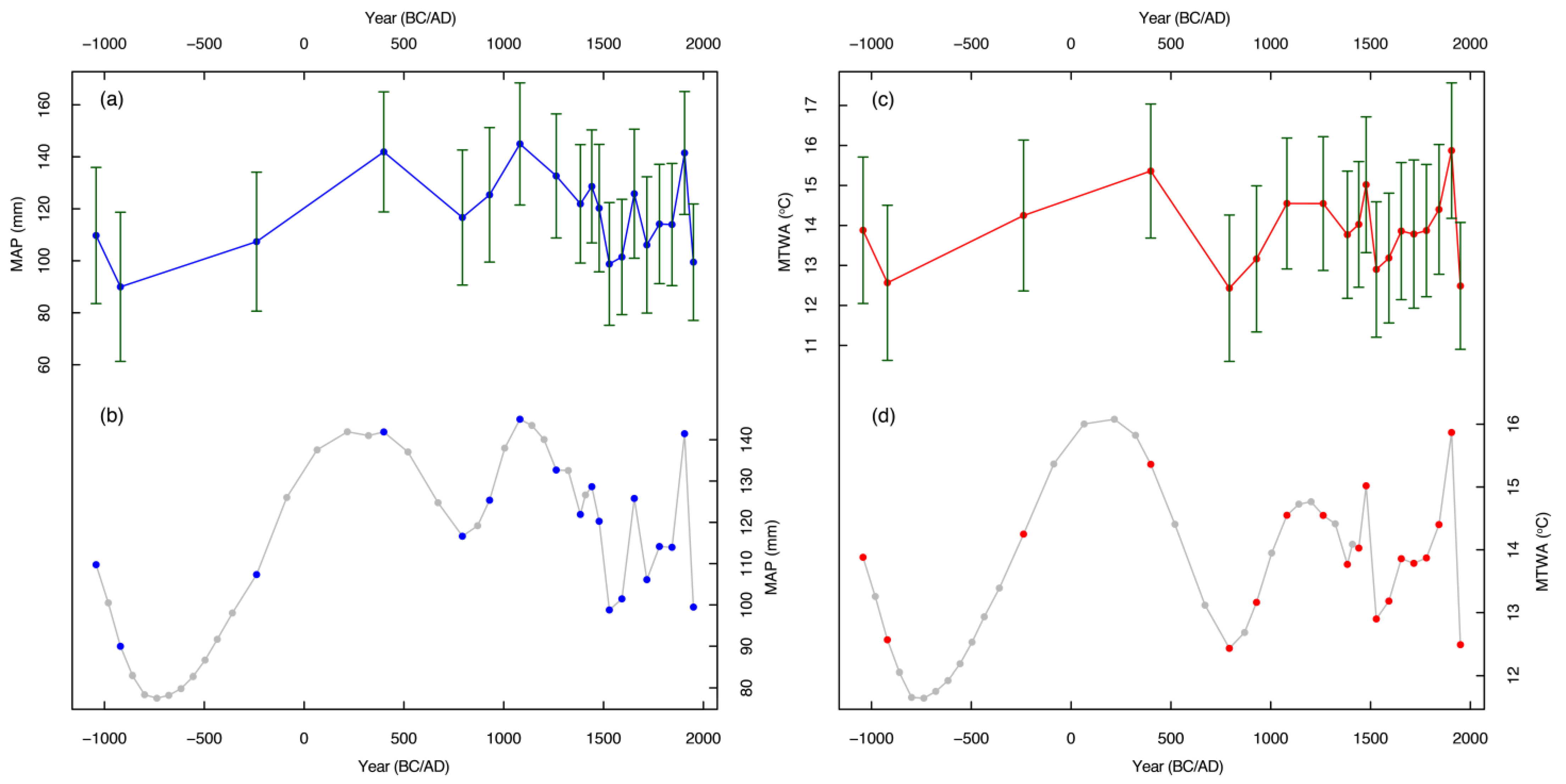
3.5. Late Holocene Quantitative Palaeoclimate Reconstructions

The successful validation of the transfer function models based on standard statistical criteria [38] shows prospects for the quantitative reconstruction of both precipitation (MAP) and temperature (MTWA) variables in the present study. This has led to the reconstruction of MAP and MTWA over 2992 cal years BP (1042 BC) for the Zemu glacier region of Yabuk, North Sikkim, eastern Himalaya (Figure 8). The application of the PLS MAP model using the sixth component to the Yabuk fossil pollen records yielded precipitation values between 98.9 and 144.9 mm. Similarly, for the PLS MTWA model using the fifth component, temperature values between 12.2 and 15.9 °C were yielded. The reconstructions showed variability during several periods as dry and wet episodes in MAP and cool and warm episodes in MTWA (Figure 8).

The reconstructed MAP showed variability during several periods as higher (wet) and lower (dry) episodes (Figure 8). The beginning of the reconstructed MAP, i.e., during 2992–2188 cal years BP (BC 1042–238), shows a lowering of precipitation, with the lowest (90 mm) in 2870 cal years BP (BC 920). The precipitation was higher in 1551 cal years BP and suddenly decreased until 1157 cal years BP (AD 793). Then, high precipitation was observed from 1021 to 742 cal years BP (AD 929–1478), with a maximum peak in 869 cal years BP (AD 1081). The precipitation was lower during 421–107 cal years BP (AD 1529–1843), ranging between 98.8 and 113.9 mm. However, in 296 cal years BP (AD 1654), the precipitation showed a higher value of 125.8 mm. During the recent phase of the reconstructed MAP, it showed an increasing trend in precipitation.

The reconstructed MTWA (Figure 8) shows variability during several periods, such as rising (warm) and lowering (cold) episodes in temperature (Figure 8). The beginning of the reconstructed MTWA, i.e., during 2870–2992 cal years BP (BC 1042–920), shows a lowering of temperature (13.9–12.6 °C). The temperature rises from 1551 to 2188 cal years BP (BC 238 to AD 399), with (14.2–15.4 °C) and then lowered (12.4–13.2 °C) during 1157–1021 cal years BP (AD 793–929). The temperature started rising in 869 cal years BP and reached its maximum in 472 cal years BP (AD 1478) at 15 °C. After this continued warming period, a gradual cooling phase was observed. The temperature slowly lowered in 421–170 cal years BP (AD 1529–1780) to (12.9–13.9 °C). The reconstructed MTWA around 107 cal years BP (AD 1843) shows the advent of warming after the preceding cold episodes.

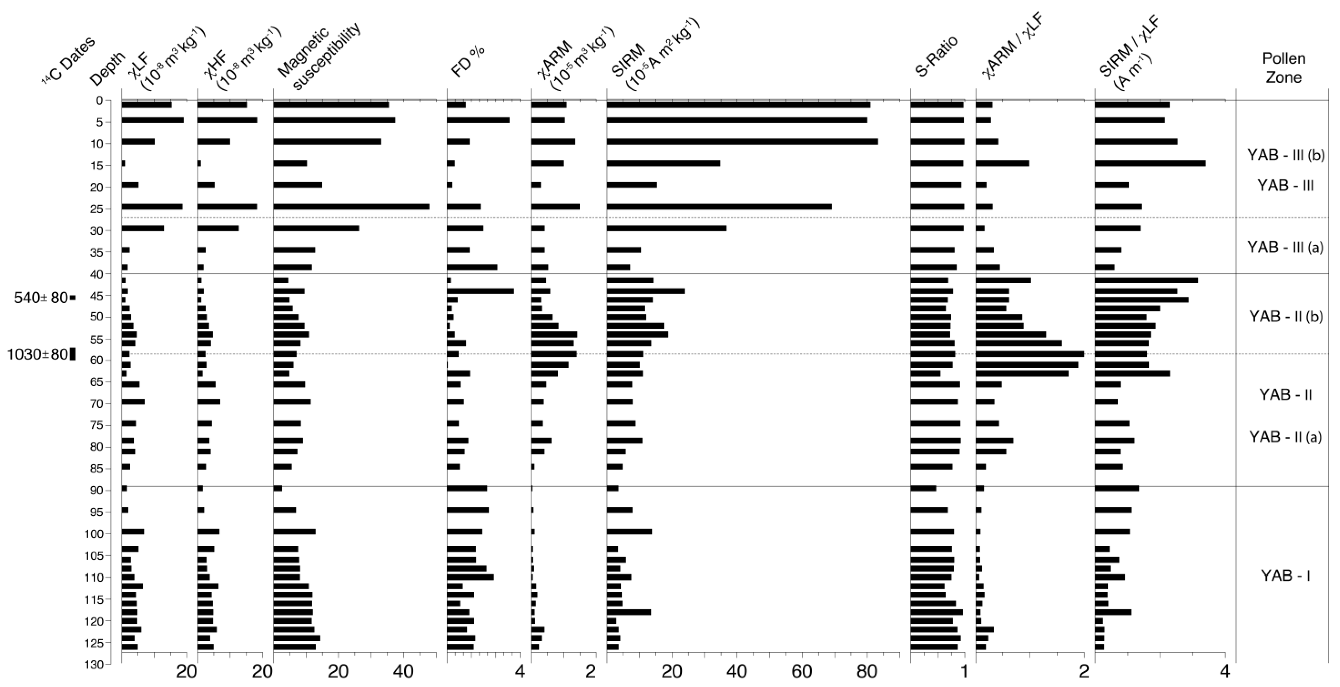
3.6. Magnetic Parameters, Fossil Pollen and Quantitative Palaeoclimate

The reconstructed quantitative precipitation and temperature records were compared with the pollen zones developed in the fossil data and supplemented with magnetic parameters, which are described in detail in Supplementary Information (Figure 9).

4. Discussion

4.1. Modern Pollen Distribution

The samples collected for modern pollen analysis have a distinct pattern of dominance of species that is also segregated also in terms of the variation in the altitude of sampling. The instances of grouping and/or clustering in both CONISS and ordination statistics following the same trends are evident. The first group (Group I) of samples or clusters included higher altitude samples (SKM90, SKM81, SKM87, SKM77, SKM101, SKM116, SKM108), occupying an altitudinal range of (3608–4300 m) and samples (SKM22) of lower altitude (2600 m). These samples showed a high dominance of alpine taxa. However, taxa such as Tsuga, Quercus pollen, and a few instances of Larix pollen were also present, probably arriving from adjoining regions.

In the second group (Group II), the samples (SKM54, SKM74, SKM65, SKM58, SKM34, SKM69, SKM39, SKM46, SKM49, SKM31, and SKM60) collected at various sites in the valley had an altitude range of 2800–3700 m. These sets of samples recorded the dominance of subalpine tree taxa, a few shrubs and herbs, and larger grass pollen and aquatic taxa. This variation in taxa can again be attributed to the lower temperatures at this altitude and increased soil moisture due to snow melt and a higher amount of precipitation. This sampling area is exposed to variable climatic conditions, allowing mixed species to appear in the sediments. However, a slight shift towards higher altitude taxa cannot be overruled. There is one sample (SKM 105), which was collected from the distant region of Chopta Valley, that has similar taxa but high levels of Rhododendron in the sample, consequently forming a separate node in the second group or cluster of samples. However, the ordination statistics and RDA imply considerations for species grouping, including climatic parameters. Hence, it is imperative that all the data and sample groups are separated not only based on the species and climate variables (MAP and MTWA), but also according to the altitude of sampling. To further strengthen the results of RDA, the CONISS results are also comparable, giving a definitive pattern to the species distribution in the region.

4.2. Pollen–Climate Relationships

The relationship between pollen assemblages and the environmental variables established using the ordination method showed the significant influence of MAP and MTWA on vegetation. The climatic variable MAP with axis 1 showed a high correlation compared to MTWA, which is slightly less correlated with axis 1, but both are statistically significant (p < 0.05). This suggests that the control of precipitation over the distribution of surface pollen could be the primary environmental driver controlling vegetation and species variations. It has been observed that sites with arid or semiarid climatic conditions, with vegetation cover and composition, are mostly controlled by moisture availability [62]. The analysis of the satellite-based normalized difference vegetation index (NDVI) compared with rainfall data from states in India showed a strong relationship between them. The study showed that NDVI is affected positively by the amount and intensity of rainfall [88]. This relationship is stronger during the monsoon season, the period that contributes the maximum percentage of water availability in annual rainfall. The NDVI precipitation result also supports the fact that precipitation has a stronger effect on vegetation distribution in the present high-elevation study area of the eastern Himalayas. In North Sikkim, precipitation in the form of rain or snow occurs throughout the year. Thus, in the present study region, precipitation has a strong influence throughout the year, which supports the present findings that highlight the significant influence of precipitation on the regional vegetation. However, in Sikkim, the rainfall/precipitation decrease sharply at higher elevations (>2000 m) in all seasons except during winter [111]. Hence, the availability of soil moisture for most taxa is high at all times, either due to rainfall or snow. However, due to the variation in altitude, the precipitation and temperature distribution at all sampling sites vary within a wide range. In the glacier region (>4000 m), the temperature decreases with snow cover, and precipitation also loses its intensity. In the cool, temperate region (2600–3300 m), both precipitation and temperature are usually at their peak during the south-west monsoon months (June to September). The rise in temperature could lead to high evapotranspiration and become the limiting factor for vegetation. The significant relationship observed with temperature could be possible, because the growth of the plants varies greatly along both latitudinal and altitudinal gradients. In the present study, the influence of both temperature and precipitation might be due to the fact that both temperature and precipitation vary greatly with altitudinal gradients. Due to this altitudinal-climatic distribution, both temperature and precipitation become the important limiting factors for the growth of plants in this region. The altitudinal influence on climate cannot be ruled out in mountainous and high-altitude regions. As the elevation increases, the temperature decreases in most of the mountainous region [4,132,133], in addition to precipitation, as also observed in the present study sites (Table S1) and reported for the entire region of Sikkim by [111]. Similar inferences on pollen–temperature–precipitation have been observed from adjoining regions such as the Tibetan Plateau, China, and Mongolia [57,59,62,134,135,136,137] on modern pollen-climate calibration, along with the statistical parameters observed in the transfer function model. The influence of precipitation as a primary environmental factor can also be explained by the fact that modern pollen sites are located in high-elevation areas with arid or semiarid climatic conditions, where vegetation cover and composition are mostly controlled by moisture availability.

4.3. Environmental Geomagnetism and Climate Reconstruction

The reconstruction of mean annual precipitation (MAP) has been based on magnetic minerals within a soil in various studies using different quantitative techniques [96,138,139,140,141,142]. Magnetic minerals such as magnetite/maghemite, hematite, and goethite abundances in soils have been identified to have a quantitative relationship with precipitation [96,142,143]. Magnetic palaeo-precipitation proxies have been studied widely in the Quaternary to recent Loess–paleosol systems in China [138,144], New Zealand [145], Alaska [146], North America [147,148,149], and Russia [150,151]. These records exhibit that the relationship between magnetic minerals and MAP differs spatio-temporally [96]. The Loess–Paleosol sequences of China have shown that variation and aeolian dust fluxes are influenced by regional monsoonal climate patterns and increases in pedogenic processes due to high precipitation and temperature [96,138,152,153,154]. Thus, the strong relationship between iron oxide mineralogy in soil sequences and climatic variations has been well established globally [96]. However, the magnetic palaeo-precipitation proxies used to estimate MAP have been said to have certain uncertainties [96,155,156].

In this study, we do not attempt a direct palaeo-precipitation reconstruction using mineral magnetic data. We have attempted to make a comparison of the reconstructed MAP using palynological data with magnetic mineral variations. Mineral magnetism data are an additional tool to identify the variations in the palaeoclimate of the Zemu glacier. Similar variations comparable to the reconstructed climate (MAP, MTWA) at Zemu glacier were found. There were many controlling factors, such as soil moisture, glacial melt, detrital deposition, podogenic processes, and regional sediment influx at the Zemu glacier. All these factors, along with the climatic parameters, control the magnetic mineral variations in the sediment. Here, the fossil pollen data also correspond to vegetation changes along with climatic variations at the Zemu glacier. The fossil pollen data in zone YAB–I is less, but an increase in the ferromagnetic mineral content is concurrent with the high MAP and MTWA and high pollen counts. In the other two zones, the vegetation gives a pattern similar to the changes in MAP and MTWA, along with the mineral magnetic. The glacier also demonstrated changes regarding the type of sediment influx at the sampling site during high precipitation periods in zones YAB–II and YAB–III, which are composed of coarse gravel with sand and silty clays. Such changes are visible in the lithology profile of the samples collected near the Zemu glacier. It is evident that material coming down from the snout of the glacier and the surrounding topography influenced the magnetic mineralogy. The vegetation, climate, and sediment flux in the valley during the Late Holocene are clearly linked together in our record. Both palynological and environmental geomagnetic data provide strong evidence of the influence of MAP and MTWA as climatic factors working in the Zemu glacier valley.

The environmental magnetism parameters are significantly low in terms of their numerical values throughout the sediment profile. They successfully capture the signals and oscillations in the environment and climate at the Zemu glacier. These parameters were analyzed for all the samples, which included samples not analyzed for palynomorphs due to the high sand content. Though we managed to obtain the entire profile data, it is possible that including all the sample data reduced the possibility of easily identifying the magnetic behavior of the minerals in the profile. However, it was important that we supported our climatic interpretation and reconstruction based on other supportive evidence.

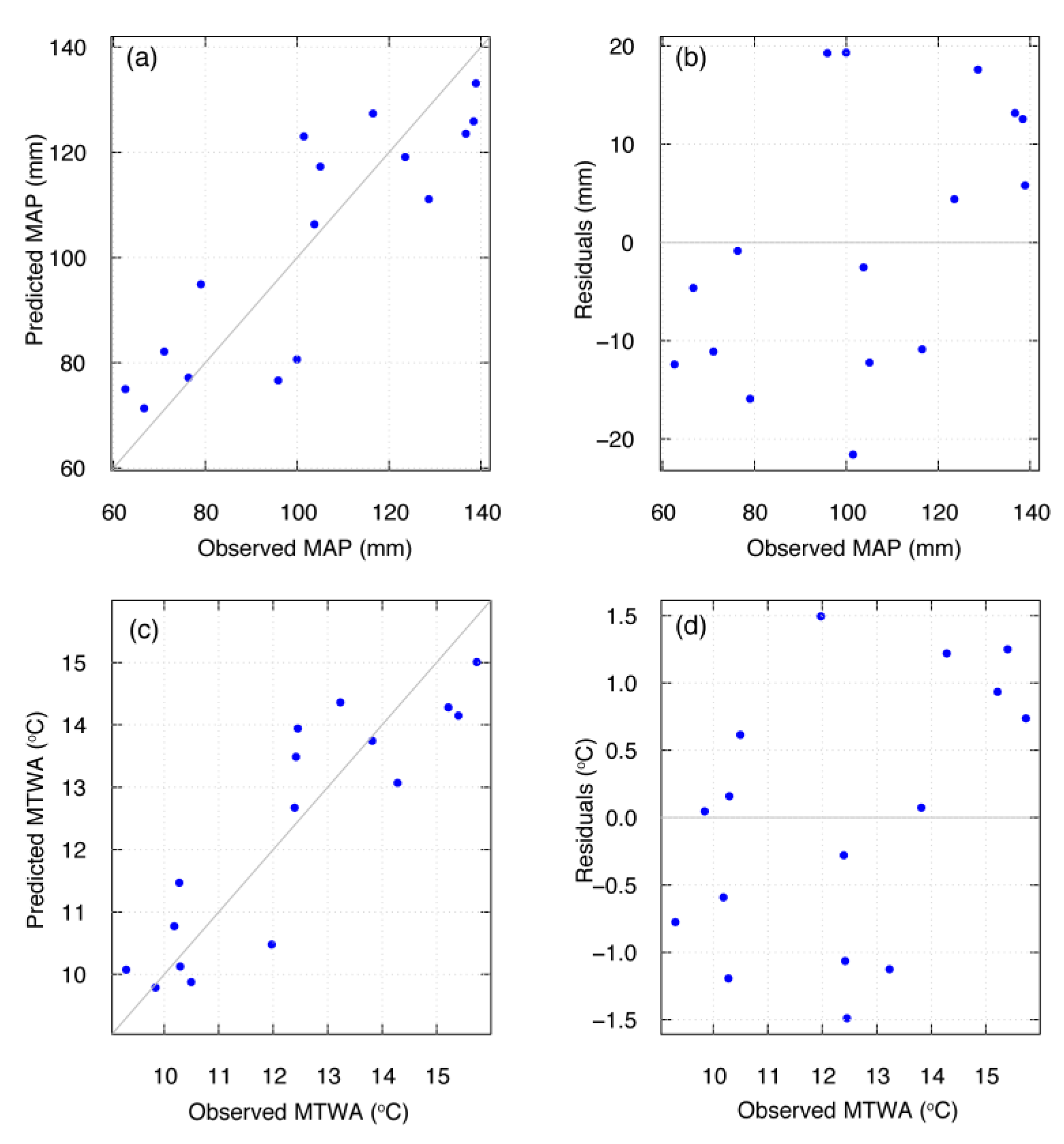
4.4. Evaluation of Climate Reconstructions

The climate of the Late Holocene, especially the last 1000–1500 years, sets the background for 20^th-century climate warming. The climate records during this period are required to perceive the natural variability in the climate system. The proxy-based long climate records emphasize the interest in quantitative climate data beyond the range of instrumental records. Long-term climate reconstructions derived from various well-dated proxy data indicate that the past millennium is the best documented interval with both historical and climate data [157]. The present pollen-based quantitative climate (MAP and MTWA) reconstructions successfully captured well-known global climate events of the recent millennium. These climatic signals helped us assess the background for recent century-long climate warming in the largest glaciated region of the eastern Himalayas.

In the present reconstructed MTWA, the high temperature covering the time span of 929–472 cal years BP (AD 1021–1478) is comparable with the MWP. After attaining a gradual rise in temperature during 509–472 cal years BP (AD 1441–1478), the significant lowering of temperature until 421 cal years BP (AD 1529) could be related to the cooling period near the beginning of the LIA. This cooling period observed in the present MTWA reconstruction is comparable with a widely known event, the Spörer Minimum, observed during AD 1460–1550 [158]. Jiang and Xu [158] clearly demonstrate that if the Spörer Minimum extended from AD 1460 to 1550, it could be a specious result; if its extent was AD 1400–1510, it could be determined as an actual feature of solar variability during that time. The slight decrease in temperature after attaining the increasing trends in our MTWA reconstruction during 296–233 cal years BP (AD 1654–1717) is comparable with a cold event widely known as the Maunder Minimum (AD 1645–1715) in the middle of the LIA [159]. The Maunder Minimum refers to a period of low solar activity [160]. The physical link between low sunspot activity and cooling temperatures has not been established, but the coincidence between the Maunder Minimum and the deepest trough of the LIA is suggestive of such a connection [161]. The present reconstructed MTWA has not captured this event significantly compared to the Spörer Minimum. Thus, the overall lowering of temperature covering a time span of 421–170 cal years BP (AD 1529–1780) suggests that the LIA event was present around the Zemu Glacier Valley. The LIA episodes observed in the reconstructed MTWA showed a sudden decrease in temperature in the early part of the initiation of the cold period, and gradually the temperature increased, with a slight decrease during the middle of the LIA. The reconstructed temperature around 107 cal years BP (AD 1843) shows the arrival of warming after the cold episodes of LIA in the Zemu glacier valley and is similar to the Current Warming Period (CWP).

The reconstructions from our records captured comparable well-known climatic events (MWP and LIA), but the timing identified is indeed not the same as that recorded in various studies (described in Section 4.5 and Section 4.6). The MWP was a time of warm climate during AD 1100–1300, which peaked in the 11th century and ended abruptly around 1300 AD [8]. Similarly, the LIA event is a known widespread climatic cooling event that lasted approximately from the 14th to the 18th centuries AD [12]. Later, Mann et al. [10] argued that MWP might be related to other climate events around the world and occur from about AD 950 to 1250, and that the cooling event LIA lasted from AD 1400 to 1700. However, Graham et al. [11] reported the duration of MCA/MWP as ca. 900–1350 AD and the LIA as ca. 1500–1850 AD. The present climate reconstruction shows cool (dry) and warm (wet) variability within the LIA and MWP, respectively. We observed cold (dry) climatic records punctuated within the ‘warm (wet)’ period of MWP. Similarly, warm (wet) records are observed during the ‘cool (dry)’ period of LIA. This illustrates the fact that ‘Medieval Warm Period’ and ‘Little Ice Age’ are moveable terms depending on region. However, the present finding supports that the worldwide climatic variability of MWP with a warm (wet) climate and LIA with cold (dry) periods also exists in this remote region of the Zemu glacier valley in the eastern Himalayas. Wanner et al. [162], based on a synthesis review of mid-to-late Holocene global climate change, concluded the existence of warm and cold periods, especially hemispheric-scale warming leading to the MWP and subsequent cooling into the LIA. The possible role of this climatic variability could be due to various natural factors. These could be fluctuations in solar activity, large tropical volcanic eruptions, internal variability in oceanic oscillations, including the El Niño Southern Oscillation (ENSO) and the North Atlantic Oscillation (NAO), changes in the thermohaline circulation, and complex feedback mechanisms between the ocean, atmosphere, sea ice, and vegetation [162]. The strong coupling between the biogenic proxies and reconstructed total solar irradiance during the last millennium from the northeastern Arabian Sea also suggested solar control on the intensity of the Indian monsoon and likely the MWP and LIA as well. Moreover, the large eruptions in the tropics and high latitudes were the primary drivers of inter-annual to decadal temperature variability in the Northern Hemisphere during the past 2500 years [163]. Based on the model simulations, Polanski et al. [157] stated that the eastern Himalayas are affected by summer variations in the temperature gradient between the Bay of Bengal and Indian subcontinent and by a zonal band of intensified Indian-East Asian monsoon link north of 25° N.

Apart from these broad global events of MWP and LIA, our climate reconstruction is also comparable with other climatic events that occurred elsewhere in the globe [164] but were not widely explained compared to MWP and LIA. These events were recorded in the reconstruction before the MWP period. The cooling of temperature at the beginning of the reconstructed MTWA (2992–2870 years BP, BC 1042–920) might be linked with the Sub-Atlantic Cold Period (SACP) that occurred during BC 975–250 [164]. The rise in temperature in the present MTWA reconstruction during 2188–1551 cal years BP (BC 238–399) is similar to the Roman Warm Period (RWP) observed during BC 250–AD 450 [164]. Another event known as the Dark Age Cold Period (DACP), which took place during AD 450–950 [164], is also comparable with the cooling events observed in our temperature reconstruction during the later part of 1157–1021 cal years BP (AD 793–929). However, we do not support the claim that these events were strongly captured in our reconstruction due to the fact that the palynological samples are smaller at the beginning of the chronology. However, at the same time, we can argue that the present reconstruction has the ability to capture climatic fluctuations that occurred during the Late Holocene elsewhere. In future studies, the observation can be strengthened with an increase in palynological sample numbers and a higher-resolution chronology. Thus, greater emphasis was given to MWP and LIA events, which were compared with other records in detail.

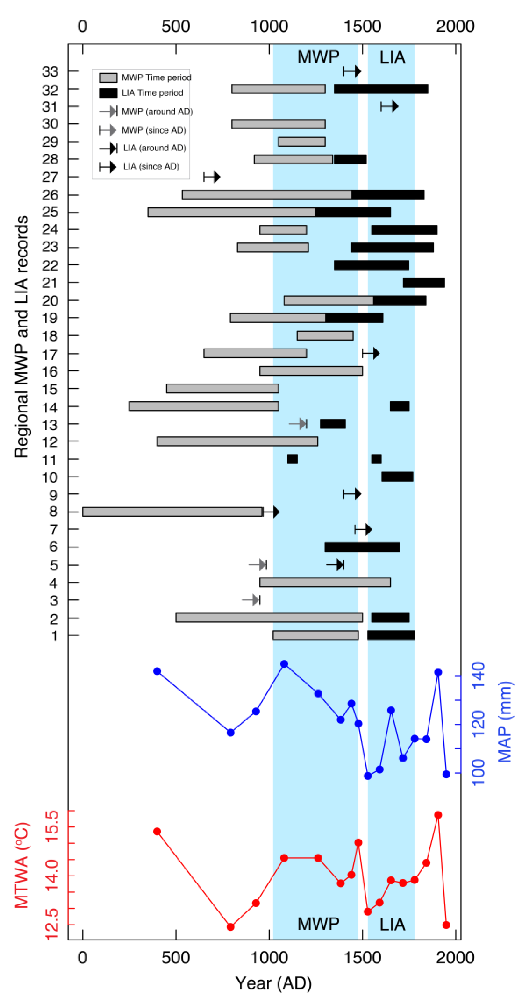
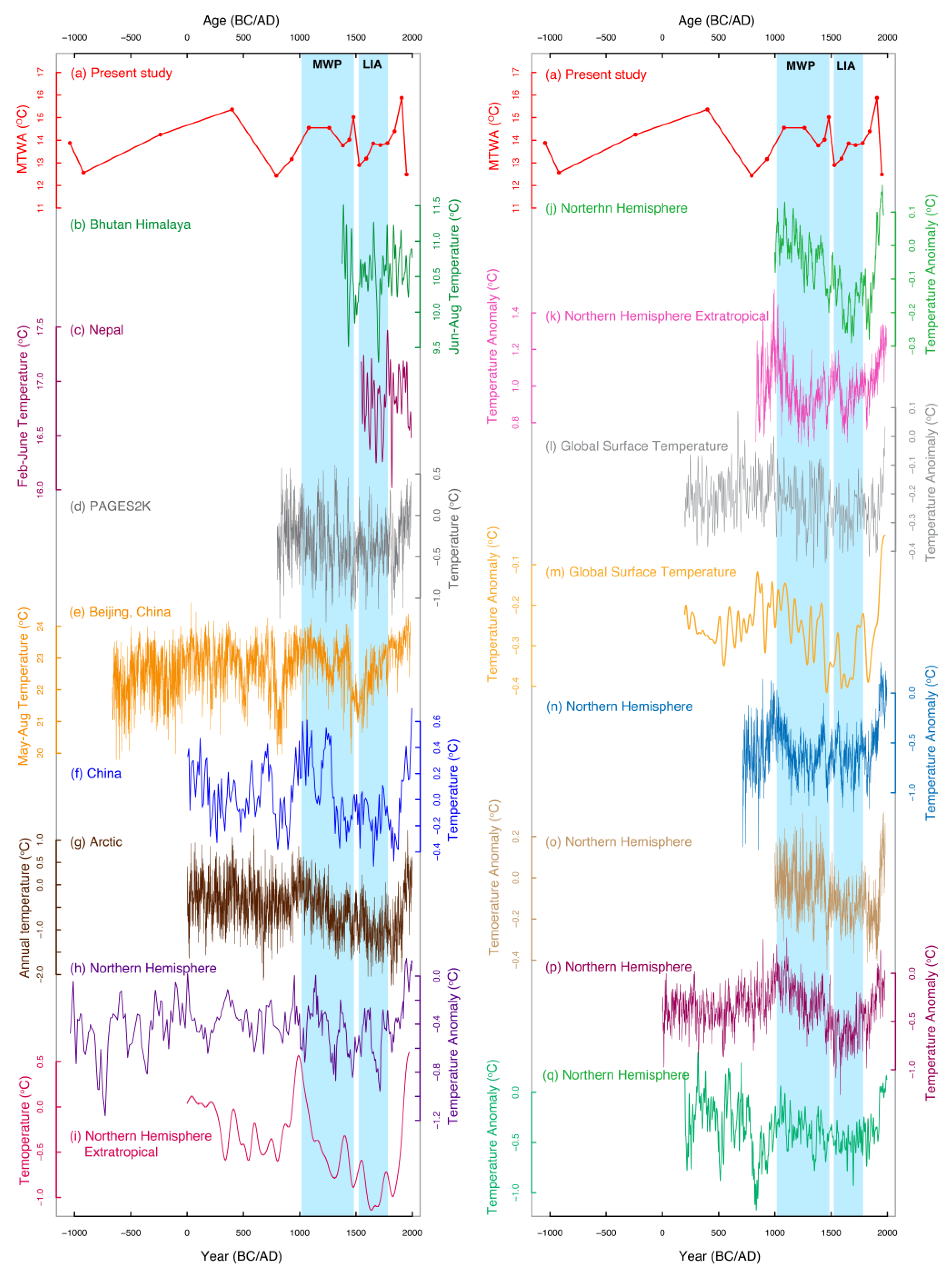
4.5. Climate Reconstructions Comparison

In the present study, we provide the first quantitative climate (precipitation and temperature) reconstruction of the Zemu glacier valley in the eastern Himalayas using the transfer function model. In order to look at our climate reconstructions of the Zemu glacier from a larger geographical perspective, we compared them with proxies-based climate reconstructions carried out in India and adjoining areas, including south Asian continents and the northern hemisphere. For this comparison, two approaches were considered: (i) qualitative climate inference made from different proxy-based studies and (ii) quantitative climate reconstruction from various proxies available from NOAA data contributors (www.ncdc.noaa.gov, accessed on 10 January 2022) and obtained from personal contribution on request. For both approaches, comparisons were made for past climatic events and variability recorded during the Late Holocene.

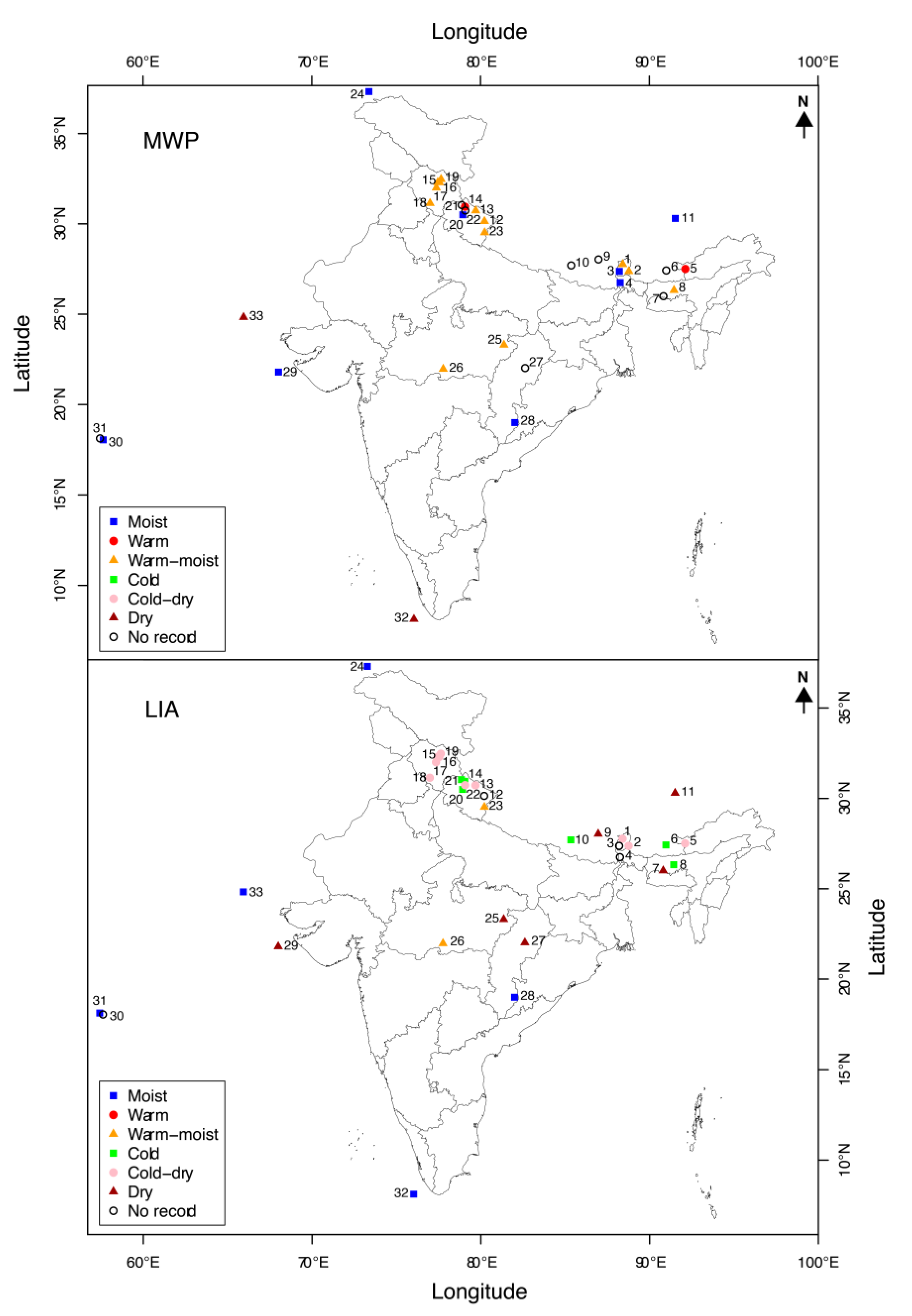
4.5.1. Climate Reconstructions Comparison—Qualitative Approach

The climatic variability during the MWP and LIA time periods recorded in the present pollen-based climate reconstructions is comparable with other pollen and proxy-based studies carried out in different regions of India, the Himalayas, and the adjoining oceanic region. The time span and climatic inference made for the MWP and LIA periods in these studies [16,84,85,87,158,165,166,167,168,169,170,171,172,173,174,175,176,177,178,179,180,181,182,183,184,185,186,187,188,189,190,191,192,193,194,195,196,197,198,199,200,201,202,203,204] are presented in Figure 10 and Figure 11, respectively, and are described in the following section. We have given an extensive explanation and comparison of these records in Supplementary Information.

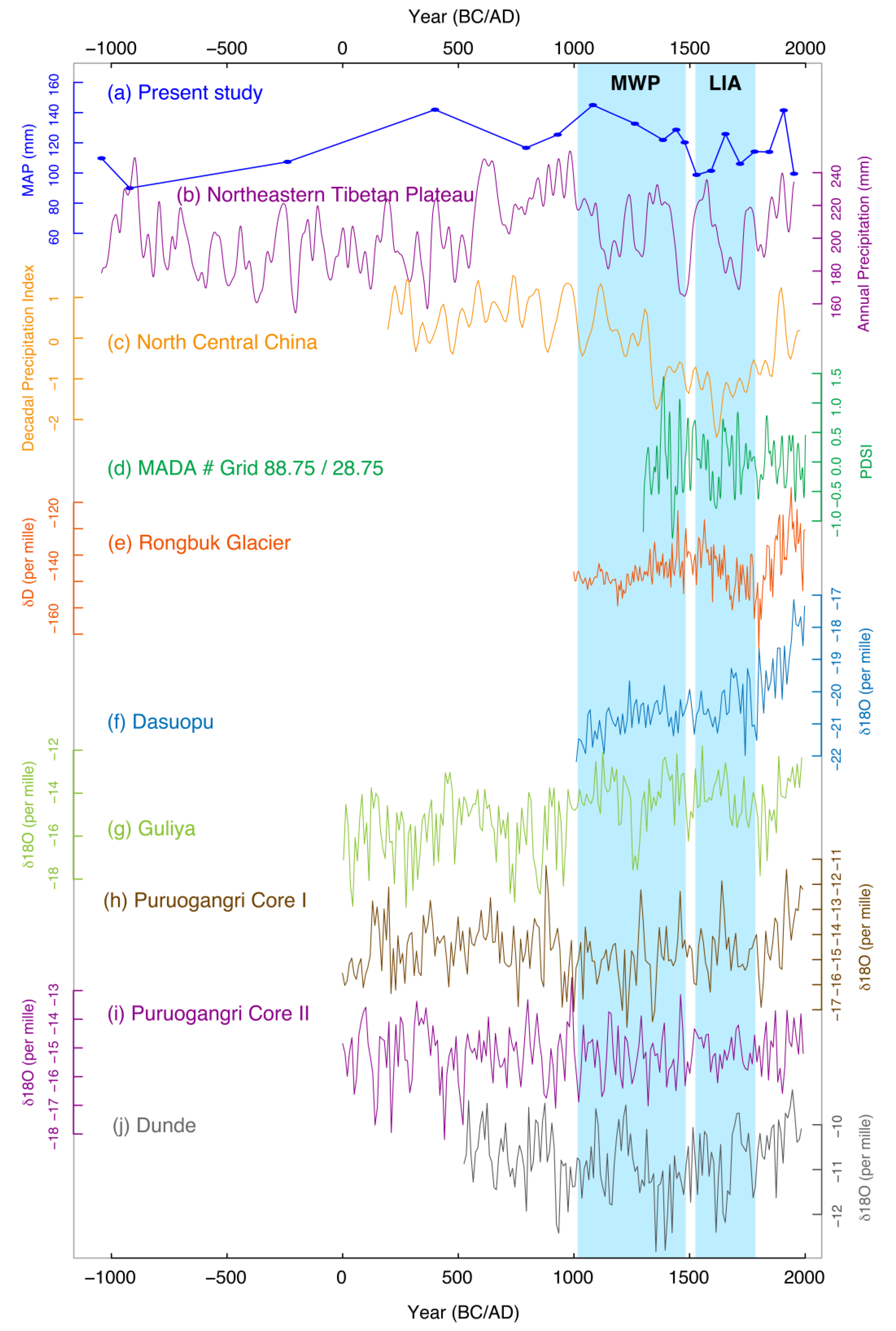
4.5.2. Climate Reconstructions Comparison—Quantitative Approach

The quantitative climate (precipitation and temperature) reconstructions developed in the present study were compared graphically with available Late Holocene reconstructions (Figure 12). For this comparison, reconstructed temperature and precipitation data using other proxy data were procured from NOAA data contributors and also provided by the author of the research paper.

The MAP reconstruction is compared with available precipitation, drought, and ice core records. The MAP is compared with 3500 years of annual precipitation reconstruction from the Northeastern Tibetan Plateau based on tree-ring data [205] and the north central China 1800-year decadal precipitation index reconstruction using stalagmite and historical document records [206] shows similar trends in the later period of MWP and LIA. The reconstructed Palmer drought severity index (PDSI) from the Monsoon Asia Drought Atlas (MADA) [207] from the nearest grid point (88.75/28.75) in the present study site also shows consistency in the trends during LIA. The MAP has been also compared with ice core records of Rongbuk Glacier [173], Dasuopu [208,209], Guliya [210], Dunde [211], and Puruogangri core I and II [212]. Apart from Puruogangri core II, all other ice core records compared with the present reconstructed MAP shows similar variability in the reconstruction.

Figure 12. Comparison of (a) reconstructed MAP (present study) with other proxy-based climate reconstruction (b) annual precipitation from northeastern Tibetan Plateau [205], (c) decadal precipitation index from northcentral China [206], (d) PDSI from Monsoon Asian Drought Atlas (MADA) [207], (e) ice core record from Rongbuk glacier, Nepal [173], (f) ice core record from Dasuopu [208,209], (g) ice core record from Guliya, Tibetan Plateau [210], (h,i) ice core record from Puruogangri core I and II [212] and (j) ice core record from Dunde [211].

Figure 12. Comparison of (a) reconstructed MAP (present study) with other proxy-based climate reconstruction (b) annual precipitation from northeastern Tibetan Plateau [205], (c) decadal precipitation index from northcentral China [206], (d) PDSI from Monsoon Asian Drought Atlas (MADA) [207], (e) ice core record from Rongbuk glacier, Nepal [173], (f) ice core record from Dasuopu [208,209], (g) ice core record from Guliya, Tibetan Plateau [210], (h,i) ice core record from Puruogangri core I and II [212] and (j) ice core record from Dunde [211].

Similarly, the present reconstructed temperature (MAT) has been compared with temperature reconstructions from adjoining areas and regional, Arctic, hemispheric and global records (Figure 13). The tree-ring-based June–August temperature reconstruction from Bhutan [16] shows cold conditions during the early 15th, 16th, and late 17th to early 18th centuries. Another tree-ring-based temperature reconstruction from Nepal [200] also shows a lowering of temperature during AD 1670–1770, which falls in the period of LIA. In addition, temperature reconstruction for Asia [213] using multi-proxy records, temperature reconstruction using stalagmite records from Beijing, China [214], temperature reconstruction in China using proxy records with methods of principal component regression and partial least squares regression [215], and Arctic-wide temperature reconstruction for the past 2000 years [216] also show comparable variability with the present reconstructed temperature. The temperature reconstructions available from various hemispheric and global levels include: multi-proxy reconstructions of the extra-tropical northern hemisphere (30–90° N) mean temperature [217]; reconstructions of northern hemisphere temperatures and climate forcing over the past 1000 years using multi-proxy records [218]; low-frequency temperature signals reconstructed using Regional Curve Standardized tree-ring chronologies from 14 sites in the northern hemisphere extra-tropics [219]; northern hemisphere high-elevation tree-ring-based temperature reconstruction using the regional curve standardization technique [220]; multi-proxy northern hemisphere temperature reconstruction using inverse regression-truncated EOF climate field reconstruction [221]; northern hemisphere temperature reconstruction calculated by combining low-resolution proxies with tree-ring data [222]; multi-proxy northern hemispheric surface temperature reconstruction [223]; and multi proxy global surface temperature [224] also show similar temperature variability to the present temperature reconstruction in different time periods, especially during MWP and LIA (Figure 13). However, the differences in variability in both the temperature and precipitation comparative analysis with the present climate reconstruction might be due to the differences in the proxy data used, the reconstructed seasons, and the resolution of the proxies.

4.6. Climate Reconstructions and Fluctuation of Sikkimese Glaciers

The present findings of LIA in the climate reconstructions might have linkages with the advances and retreats of the Zemu glacier and other glaciers in Sikkim, Himalaya. In 1995, a study team at the Khangchendzonga Biosphere Reserve reported that since the LIA, the Zemu glacier, Onglokthang glacier, and Rathong Chu glacier in North Sikkim had retreated by 3–4 km, ~500 m, and ~600 m, respectively [225]. A similar response of the cold and dry period of climate on glacier advancement has been recorded in the glacier region of Sithikher Bog, western Himalayas [179], and the Sonapani glacier advance stage II in the Lahaul valley, western Himalayas [226]. The climate reconstruction from this largest glacier of the eastern Himalayas also shows consistency with the climatic observations of the Late Holocene made from the other largest glacier of the western Himalayas [177]. Chaujar [186] also reported that the northern and southern hemispheric glaciers started their retreat in the mid-18th century, which indicates the end of the LIA climatic period. This temporal linkage suggests the possible existence of a common trend in the mountain regions of both hemispheres and the Himalayas, and, thus, its occurrence is a global phenomenon.

Observations made during the early 1940s and 1970s [106,227,228] also suggested the expansion and then receding of the Zemu glacier. The valley has its maximum depth at the center, where the thickness of the glacier ice exceeds 300 m. This suggests that the glacier once occupied the entire valley, extending from the northern to the southern rock walls, and that it has undergone considerable lateral shrinkage, giving rise to the northern and southern trenches. Subsequent movement of the glacier, confined by the lateral moraine ridges, has eroded the bedrock to a greater extent in the central zone than that underlying the trenches from which the glacier has receded to its present position [106].

The Zemu Glacier, located in in Sikkim, the Himalayas, which was visited by the 2nd German Himalaya Expedition in 1931, has been receding since 1891 [227,228], which correlates with evidence from our records of warming trends in temperature. These observations support the evidence of LIA-like events and recent warming phases recorded in our quantitative temperature reconstruction.

The climate oscillation recorded in the present climate reconstruction, especially during the well-known global climate periods of MWP (warm–humid climate) and LIA (cold–dry climate), could be related to glacier behavior and tree line fluctuations. During the warm and humid period, the glaciers might have retreated in this region, and, as a consequence, tree line might ascend to higher elevations. During the cold–dry period, the glacier of this region as well as the tree line might have advanced towards the lower elevations. Thus, the pollen-based climate reconstruction from the glacier region enabled a chronology of glacier activity for the LIA and more recent periods to be established.

The model simulations support the suggestion that the LIA may have been brought about by low northern hemisphere orbital forcing during the Late Holocene, with coincidentally unusually low solar activity and a high number of major volcanic events [162]. So, we can contemplate that this region of the Himalaya was also influenced by solar fluctuations and volcanic activities that occurred elsewhere during the LIA period. The tree-ring studies carried out in the adjacent Bhutan Himalaya [16] also reported that the cooling of the climate during LIA was influenced by solar and volcanic eruptions.

5. Conclusions

The calibration set for modern pollen–climate (temperature and precipitation) provided the development of quantitative climate reconstructions from sub-surface sediment pollen spectra from the Zemu glacier region, eastern Himalayas. The development of a transfer function model using a linear model based on Partial Least Square regression led to the reconstruction of the mean annual precipitation (MAP) and the mean temperature of the warmest month (MTWA). Precipitation has the strongest influence on the composition of the modern pollen samples among the other climatic variables considered in the analysis. The climate reconstruction based on pollen data, supplemented with environmental magnetism analysis, cumulatively indicates the changing climatic scenario around the Zemu Glacier during the later part of the Holocene. In the absence of long-term instrumental records from this largest glacier region of the eastern Himalayas, proxy-based quantitative climate reconstructions provide an understanding of the relative contribution of changes in temperature and precipitation in glacier environments. The present study provided valuable insight into past precipitation and temperature changes, which helped us identify shifts in climatic conditions as demonstrated by various research outputs, from regional to hemispheric. The climatic variability reconstructed in this study clearly demonstrates close agreement between oscillatory climatic phenomena of the past in the region of the North Atlantic Ocean and the distant Himalayas. Our climate reconstructions capture well-documented world-wide climatic events, such as the MWP and LIA, as well as those of the even earlier Dark Ages Cold Period and Roman Warm Period. Since the present climate reconstructions have been carried out at a remote location in the largest glaciated region of the eastern Himalayas, the observed warming during the late 19^th century and then the cooling trend during the early 20th century are most likely of natural origin and not due to any anthropogenic influences. The overall assessment of quantitative climate reconstruction in the Zemu glacier area and its temporal trends, which are comparable with regional, continental, hemispheric perspectives and from a global perspective, should look forward to a more comprehensive analysis with both spatial and temporal coverage.

References

1. Sarntheina, M.; Kennett, J.P.; Allen, J.R.M.; Beer, J.; Grootes, P.; Laj, C.; McManus, J.; Ramesh, R.; SCOR—IMAGES Working Group 117. Decadal–to–millennial–scale climate variability—Chronology and mechanisms: Summary and recommendations. Quat. Sci. Rev. 2002, 21, 1121–1128. [Google Scholar] [CrossRef]
2. Bradley, R.S. Past global changes and their significance for the future. Quat. Sci. Rev. 2000, 19, 391–402. [Google Scholar] [CrossRef]
3. Beniston, M. Climate Change in Mountain Regions: A Review of Possible Impacts. Clim. Chang. 2003, 59, 5–31. [Google Scholar] [CrossRef]
4. Whiteman, D. Mountain Meteorology; Oxford University Press: New York, NY, USA, 2000; p. 355. [Google Scholar]
5. Thompson, L.G. Ice core evidence for climate changes in the Tropics: Implications for our future. Quat. Sci. Rev. 2000, 19, 19–35. [Google Scholar] [CrossRef]
6. Lowe, J.J.; Walker, M.J.C. Reconstructing Quaternary Environments, 2nd ed.; Longman Asia Limited: Hong Kong, China, 2015. [Google Scholar]
7. Bradley, R.S. Paleoclimatology: Reconstructing Climates of the Quaternary, 3rd ed.; Elsevier/Academic Press: San Diego, CA, USA, 2014; p. 675. [Google Scholar]
8. Lamb, H. The early medieval warm epoch and its sequel. Palaeogeogr. Palaeoclim. Palaeoecol. 1965, 1, 13–37. [Google Scholar] [CrossRef]
9. Stine, S. Medieval climatic anomaly in the Americas. In Water, Environment and Society in Times of Climatic Change; Issar, A.S., Brown, N., Eds.; Kluwer: Dordrecht, The Netherlands, 1998; pp. 43–67. [Google Scholar]
10. Mann, M.E.; Zhang, Z.; Rutherford, S.; Bradley, R.S.; Hughes, M.K.; Shindell, D.; Ammann, C.; Faluvegi, G.; Ni, F. Global signatures and dynamical origins of the little ice age and Wanner medieval climate anomaly. Science 2009, 326, 1256–1260. [Google Scholar] [CrossRef] [PubMed]
11. Graham, N.E.; Ammann, C.M.; Fleitmann, D.; Cobb, K.M.; Luterbacher, J. Support for global climate reorganization during the “Medieval Climate Anomaly”. Clim. Dyn. 2010, 37, 1217–1245. [Google Scholar] [CrossRef]
12. Grove, J.M. The Little Ice Age; Methuen: London, UK, 1988. [Google Scholar]
13. Bhattacharyya, A.; Shah, S.K. Tree–ring study in India—Past appraisal, present status and future prospects. IAWA 2009, 30, 361–370. [Google Scholar] [CrossRef]
14. Bhattacharyya, A.; Chaudhary, V. Late-Summer Temperature Reconstruction of the Eastern Himalayan Region Based on Tree-Ring Data of Abies densa. Arct. Antarct. Alp. Res. 2003, 35, 196–202. [Google Scholar] [CrossRef]
15. Shah, S.K.; Mehrotra, N.; Bhattacharyya, A. Tree ring studies from Eastern Himalaya: Prospects and challenges. Him. Res. J. 2014, 2, 21–28. [Google Scholar]
16. Krusic, P.J.; Cook, E.R.; Dukpa, D.; Putnam, A.E.; Rupper, S.; Schaefer, J. Six hundred thirty-eight years of summer temperature variability over the Bhutanese Himalaya. Geophys. Res. Lett. 2015, 42, 2988–2994. [Google Scholar] [CrossRef]
17. Birks, H.J.B. The use of pollen analysis in the reconstruction of past climates: A review. In Climate and History; Wigley, T.M.L., Ingram, M.J., Farmer, G., Eds.; Cambridge University Press: Cambridge, UK, 1981; pp. 111–138. [Google Scholar]
18. Huntley, B. Quaternary palaeoecology and ecology. Quat. Sci. Rev. 1996, 15, 591–606. [Google Scholar] [CrossRef]
19. Birks, H.J.B. Numerical analysis methods. In Encyclopedia of Quaternary Science; Elias, S., Ed.; Elsevier: Amsterdam, The Netherlands, 2007; pp. 2514–2521. [Google Scholar]
20. Brewer, S.; Guiot, J.; Barboni, D. Use of pollen as climate proxies. In Encyclopedia of Quaternary Science; Elias, S., Ed.; Elsevier: Amsterdam, The Netherlands, 2007; pp. 2497–2508. [Google Scholar]
21. Edwards, M.E. BIOME model of vegetation reconstruction. In Encyclopedia of Quaternary Science; Elias, S., Ed.; Elsevier: Amsterdam, The Netherlands, 2007; pp. 2551–2561. [Google Scholar]
22. Seppä, H. Pollen analysis, Principles. In Encyclopedia of Quaternary Science; Elias, S., Ed.; Elsevier: Amsterdam, The Netherlands, 2007; pp. 2486–2497. [Google Scholar]
23. Bhattacharyya, A.; Ranhotra, P.S.; Shah, S.K. Temporal and spatial variations of late Pleistocene–Holocene climate of the western Himalaya based on pollen records and their implications to Monsoon dynamics. J. Geol. Soc. India 2006, 68, 507–515. [Google Scholar]
24. Bhattacharyya, A.; Ranhotra, P.S.; Shah, S.K. Spatio Temporal Variation of Alpine Vegetation vis–à–vis Climate during Holocene in the Himalaya. Mem. Geol. Soc. India 2011, 77, 309–319. [Google Scholar]
25. Mehrotra, N.; Shah, S.K.; Bhattacharyya, A. Review of palaeoclimate records from Northeast India based on pollen proxy data of Late Pleistocene–Holocene. Quat. Int. 2014, 325, 41–54. [Google Scholar] [CrossRef]
26. Seppä, H.; Bennett, K.D. Quaternary pollen analysis: Recent progress in palaeoecology and palaeoclimatology. Prog. Phys. Geogr. 2003, 27, 548–579. [Google Scholar] [CrossRef]
27. Iversen, J. Viscum, Hedera and Ilex as climatic indicators. A contribution to the study of the post–glacial temperature climate. Geol. Föreningens I Stockh. Förhandlingar 1944, 66, 463–483. [Google Scholar] [CrossRef]
28. Grichuk, V.P. An experiment in reconstructing some characteristics of climate in the Northern Hemisphere during the Atlantic Period of Holocene. In Holocene; Neustadt, M.I., Ed.; Nauka: Moscow, Russia, 1969; pp. 41–57. [Google Scholar]
29. Tarasov, P.E.; Nakagawa, T.; Demske, D.; Österle, H.; Igarashi, Y.; Kitagawa, J.; Mokhova, L.; Bazarova, V.; Okuda, M.; Gotanda, K.; et al. Progress in the reconstruction of Quaternary climate dynamics in the Northwest Pacific: A new modern analogue reference dataset and its application to the 430-kyr pollen record from Lake Biwa. Earth Sci. Rev. 2011, 108, 64–79. [Google Scholar] [CrossRef]
30. Imbrie, J.; Kipp, N.G. A new micropaleontological method for quantitative paleoclimatology: Application to a late Pleistocene Caribbean core. In The Late Cenozoic Glacial Ages; Turekian, K.K., Ed.; Yale University Press: New Haven, CT, USA, 1971; pp. 71–181. [Google Scholar]
31. Webb, I.I.I.T.; Thompson, B.; Bryson, R.A. Late-and postglacical climatic change in the northern Midwest, USA: Quantitative estimates from fossil pollen spectra by multivariate statistical analysis. Quat. Res. 1972, 2, 70–115. [Google Scholar] [CrossRef]
32. Bartlein, P.J.; Webb, T.I.I.I.; Fleri, E. Holocene climatic change in the northern Midwest: Pollen–derived estimates. Quat. Res. 1984, 22, 361–374. [Google Scholar] [CrossRef]
33. Bartlein, P.J.; Webb, T.I.I.I. Mean July temperature at 6000 yr B.P. in eastern North America: Regression equations for estimates from fossil–pollen data. Syllogeus 1985, 55, 301–342. [Google Scholar]
34. Guiot, J. Late Quaternary Climatic Change in France Estimated from Multivariate Pollen Time Series. Quat. Res. 1987, 28, 100–118. [Google Scholar] [CrossRef]
35. Huntley, B.; Prentice, I.C. July temperature in Europe from pollen data, 6000 years before present. Science 1988, 241, 687–690. [Google Scholar] [CrossRef]
36. Guiot, J.; Pons, A.; de Beaulieu, J.-L.; Reille, M. A 140,000–year climatic reconstruction from two European pollen records. Nature 1989, 338, 309–313. [Google Scholar] [CrossRef]
37. ter Braak, C.J.F.; Juggins, S. Weighted averaging partial least squares regression (WA–PLS): An improved method for reconstruction environmental variables from species assemblages. Hydrobiologia 1993, 269, 485–502. [Google Scholar] [CrossRef]
38. Birks, H.J.B. Quantitative palaeoenvironmental reconstructions. In Statistical Modelling of Quaternary Science Data; Maddy, D., Brew, J.S., Eds.; Quaternary Research Association: Cambridge, UK, 1995; pp. 161–254. [Google Scholar]
39. Peyron, O.; Guiot, J.; Cheddadi, R.; Tarasov, P.E.; Reille, M.; deBeaulieu, J.-L.; Bottema, S.; Andrieu, V. Climatic reconstruction in Europe from pollen data, 18,000 years before present. Quat. Res. 1998, 49, 183–196. [Google Scholar] [CrossRef]
40. Seppä, H.; Birks, H.J.B. July mean temperature and annual precipitation trends during the Holocene in the Fennoscandian tree–line area, pollen–based reconstructions. Holocene 2001, 11, 527–539. [Google Scholar] [CrossRef]
41. Seppä, H.; Birks, H. Holocene Climate Reconstructions from the Fennoscandian Tree-Line Area Based on Pollen Data from Toskaljavri. Quat. Res. 2002, 57, 191–199. [Google Scholar] [CrossRef]
42. Markgraf, V.; Webb, R.S.; Anderson, K.H.; Anderson, L. Modern pollen/climate calibration for southern South America. Palaeogeogr. Palaeoclimatol. Palaeoecol. 2002, 181, 375–397. [Google Scholar] [CrossRef]
43. Davis, B.; Brewer, S.; Stevenson, A.; Guiot, J. The temperature of Europe during the Holocene reconstructed from pollen data. Quat. Sci. Rev. 2003, 22, 1701–1716. [Google Scholar] [CrossRef]
44. Seppä, H.; Birks, H.J.B.; Odland, A.; Poska, A.; Veski, S. A modern pollen-climate calibration set from northern Europe: Developing and testing a tool for palaeoclimatological reconstructions. J. Biogeogr. 2004, 31, 251–267. [Google Scholar] [CrossRef]
45. Seppä, H.; Hammarlund, D.; Antonsson, K. Low–frequency and high frequency changes in temperature and effective humidity during the Holocene in south–central Sweden, implications for atmospheric and oceanic forcings of climate. Clim. Dyn. 2005, 25, 285–297. [Google Scholar] [CrossRef]
46. Seppä, H.; MacDonald, G.M.; Birks, H.J.B.; Gervais, B.R.; Snyder, J.A. Late-Quaternary summer temperature changes in the northern-European tree-line region. Quat. Res. 2008, 69, 404–412. [Google Scholar] [CrossRef]
47. Seppä, H.; Bjune, A.E.; Telford, R.J.; Birks, H.J.B.; Veski, S. Last nine-thousand years of temperature variability in Northern Europe. Clim. Past 2009, 5, 523–535. [Google Scholar] [CrossRef]
48. Tarasov, P.; Granoszewski, W.; Bezrukova, E.; Brewer, S.; Nita, M.; Abzaeva, A.; Oberhänsli, H. Quantitative reconstruction of the last interglacial vegetation and climate based on the pollen record from Lake Baikal, Russia. Clim. Dyn. 2005, 25, 625–637. [Google Scholar] [CrossRef]
49. Tarasov, P.E.; Bezrukova, E.V.; Krivonogov, S.K. Late glacial and Holocene changes in vegetation cover and climate in southern Siberia derived from a 15 kyr long pollen record from Lake Kotokel. Clim. Past. 2009, 5, 73–84. [Google Scholar] [CrossRef]
50. Peros, M.C.; Gajewski, K. Holocene climate and vegetation change on Victoria Island, western Canadian Arctic. Quat. Sci. Rev. 2008, 27, 235–249. [Google Scholar] [CrossRef]
51. Dormoy, I.; Peyron, O.; Nebout, N.C.; Goring, S.; Kotthoff, U.; Magny, M.; Pross, J. Terrestrial climate variability and seasonality changes in the Mediterranean region between 15 000 and 4000 years BP deduced from marine pollen records. Clim. Past 2009, 5, 615–632. [Google Scholar] [CrossRef]
52. Litt, T.; Schölzel, C.; Kühl, N.; Brauer, A. Vegetation and climate history in the Westeifel Volcanic Field (Germany) during the past 11 000 years based on annually laminated lacustrine maar sediments. Boreas 2009, 38, 679–690. [Google Scholar] [CrossRef]
53. Bartlein, P.J.; Harrison, S.; Brewer, S.; Connor, S.; Davis, B.A.S.; Gajewski, K.; Guiot, J.; Harrison-Prentice, T.I.; Henderson, A.P.; Peyron, O.; et al. Pollen-based continental climate reconstructions at 6 and 21 ka: A global synthesis. Clim. Dyn. 2011, 37, 775–802. [Google Scholar] [CrossRef]
54. Nakagawa, T.; Tarasov, P.E.; Nishida, K.; Gotanda, K.; Yasuda, Y. Quantitative pollen-based climate reconstruction in central Japan: Application to surface and Late Quaternary spectra. Quat. Sci. Rev. 2002, 21, 2099–2113. [Google Scholar] [CrossRef]
55. Nakagawa, T.; Kitagawa, H.; Yasuda, Y.; Tarasov, P.E.; Kotoba, N.; Gotanda, K.; Sawai, Y.; Program, Yangtze River Civilization. Asynchronous Climate Changes in the North Atlantic and Japan During the Last Termination. Science 2003, 299, 688–691. [Google Scholar] [CrossRef] [PubMed]
56. Jiang, W.; Guo, Z.; Sun, X.; Wu, H.; Chu, G.; Yuan, B.; Hatté, C.; Guiot, J. Reconstruction of climate and vegetation changes of Lake Bayanchagan (Inner Mongolia): Holocene variability of the East Asian monsoon. Quat. Res. 2006, 65, 411–420. [Google Scholar] [CrossRef]
57. Shen, C.; Liu, K.-B.; Tang, L.; Overpeck, J.T. Quantitative relationships between modern pollen rain and climate in the Tibetan Plateau. Rev. Palaeobot. Palynol. 2006, 140, 61–77. [Google Scholar] [CrossRef]
58. Tarasov, P.; Jin, G.; Wagner, M. Mid-Holocene environmental and human dynamics in northeastern China reconstructed from pollen and archaeological data. Palaeogeogr. Palaeoclim. Palaeoecol. 2006, 241, 284–300. [Google Scholar] [CrossRef]
59. Li, Y.; Xu, Q.; Liu, J.; Yang, X.; Nakagawa, T. A transfer-function model developed from an extensive surface-pollen data set in northern China and its potential for palaeoclimate reconstructions. Holocene 2007, 17, 897–905. [Google Scholar] [CrossRef]
60. Zhu, C.; Chen, X.; Zhang, G.S.; Ma, C.M.; Zhu, Q.; Li, Z.X.; Xu, W.F. Spore pollen–climate factor transfer function and paleoenvironment reconstruction in Dajiuhu, Shennongjia, Central China. Chin. Sci. Bull. 2008, 53, 42–49. [Google Scholar] [CrossRef]
61. Herzschuh, U.; Kramer, A.; Mischke, S.; Zhang, C. Quantitative climate and vegetation trends since the late glacial on the northeastern Tibetan Plateau deduced from Koucha Lake pollen record. Quat. Res. 2009, 71, 162–171. [Google Scholar] [CrossRef]
62. Herzschuh, U.; Birks, H.J.B.; Mischke, S.; Zhang, C.; Böhner, J. A modern pollen-climate calibration set based on lake sediments from the Tibetan Plateau and its application to a Late Quaternary pollen record from the Qilian Mountains. J. Biogeogr. 2010, 37, 752–766. [Google Scholar] [CrossRef]
63. Xu, Q.; Xiao, J.; Li, Y.; Tian, F.; Nakagawa, T. Pollen–Based Quantitative Reconstruction of Holocene Climate Changes in the Daihai Lake Area, Inner Mongolia, China. J. Clim. 2010, 23, 2856–2867. [Google Scholar] [CrossRef]
64. Park, J. A modern pollen–temperature calibration data set from Korea and quantitative temperature reconstructions for the Holocene. Holocene 2011, 21, 1125–1135. [Google Scholar] [CrossRef]
65. Sun, A.; Feng, Z. Holocene climatic reconstructions from the fossil pollen record at Qigai Nuur in the southern Mongolian Plateau. Holocene 2013, 23, 1391–1402. [Google Scholar] [CrossRef]
66. Wen, R.; Xiao, J.; Ma, Y.; Feng, Z.; Li, Y.; Xu, Q. Pollen–climate transfer functions intended for temperate eastern Asia. Quat. Int. 2013, 311, 3–11. [Google Scholar] [CrossRef]
67. Birks, H.J.B. Numerical tools in palaeolimnology—Progress, potentialities, and problems. J. Paleolimnol. 1998, 20, 307–332. [Google Scholar] [CrossRef]
68. Birks, H.J.B.; Seppä, H. Pollen–based reconstructionsof late–Quaternary climate in Europe—Progress, problems, and pitfalls. Acta Palaeobot. 2004, 44, 317–334. [Google Scholar]
69. Kumke, T.; Schölzel, C.; Hense, A. Transfer functions for palaeoclimate reconstructions—Theory and methods. In The Climate in Historical Times; Fischer, H., Kumke, T., Lohmann, G., Flöser, G., Miller, H., von Storch, H., Negendank, J.F.W., Eds.; Springer: Berlin, Germany, 2004; pp. 229–243. [Google Scholar]
70. John, H.; Birks, B. Quantitative palaeoenvironmental reconstructions from Holocene Biological data. In Global Change in the Holocene; Mackay, A., Rick, B., Birks, J., Oldfield, F., Eds.; Arnold: London, UK, 2005; p. 528. [Google Scholar]
71. Telford, R.; Birks, H. The secret assumption of transfer functions: Problems with spatial autocorrelation in evaluating model performance. Quat. Sci. Rev. 2005, 24, 2173–2179. [Google Scholar] [CrossRef]
72. Guiot, J.; de Vernal, A. Transfer functions: Methods for quantitative paleoceanography based on microfossils. In Developments in Marine Geology 1—Proxies in Late Cenozoic Paleoceanography; Hillaire Marcel, C., de Vernal, A., Eds.; Elsevier: Amsterdam, Netherlands, 2007; pp. 523–563. [Google Scholar]
73. Guiot, J. Transfer Functions. IOP Conf. Ser. Earth Environ. Sci. 2011, 14, 1–6. [Google Scholar] [CrossRef]
74. Juggins, S.; Birks, H.J.B. Quantitative environmental reconstructions from biostratigraphical data. In Tracking Environmental Change Using Lake Sediments Data Handling and Numerical Techniques; Birks, H.J.B., Lotter, A.F., Juggins, S., Smol, J.P., Eds.; Springer: Dordrecht, The Netherlands, 2011; Volume 5. [Google Scholar]
75. Lu, H.; Wu, N.; Liu, K.-B.; Zhu, L.; Yang, X.; Yao, T.; Wang, L.; Li, Q.; Liu, X.; Shen, C.; et al. Modern pollen distributions in Qinghai–Tibetan Plateau and the development of transfer functions for reconstructing Holocene environmental changes. Quat. Sci. Rev. 2011, 30, 947–966. [Google Scholar] [CrossRef]
76. Ohlwein, C.; Wahl, E.R. Review of probabilistic pollen-climate transfer methods. Quat. Sci. Rev. 2012, 31, 17–29. [Google Scholar] [CrossRef]
77. Birks, H.J.B. Numerical methods for the analysis of diatom assemblage data. In The Diatoms—Applications for the Environmental and Earth Sciences; Smol, J.P., Stoermer, E.F., Eds.; Cambridge University Press: Cambridge, UK, 2010; pp. 23–54. [Google Scholar]
78. Ghosh, R.; Paruya, D.K.; Khan, M.A.; Chakraborty, S.; Sarkar, A.; Bera, S. Late Quaternary climate variability and vegetation response in Ziro Lake Basin, Eastern Himalaya: A multiproxy approach. Quat. Int. 2014, 325, 13–29. [Google Scholar] [CrossRef]
79. Ghosh, R.; Bera, S.; Sarkar, A.; Paruya, D.K.; Yao, Y.F.; Li, C.S. ~50 ka record of monsoonal variability in the Darjeeling foothill region, eastern Himalayas. Quat. Sci. Rev. 2015, 114, 100–115. [Google Scholar] [CrossRef]
80. Mosbrugger, V.; Utescher, T. The coexistence approach—A method for quantitative reconstructions of Tertiary terrestrial palaeoclimate data using plant fossils. Palaeogeogr. Palaeoclim. Palaeoecol. 1997, 134, 61–86. [Google Scholar] [CrossRef]
81. Utescher, T.; Bruch, A.; Erdei, B.; François, L.; Ivanov, D.; Jacques, F.; Kern, A.; Liu, Y.-S.; Mosbrugger, V.; Spicer, R. The Coexistence Approach—Theoretical background and practical considerations of using plant fossils for climate quantification. Palaeogeogr. Palaeoclim. Palaeoecol. 2014, 410, 58–73. [Google Scholar] [CrossRef]
82. Sun, N.; Li, X.Q. The quantitative reconstruction of the palaeoclimate between 5200 and 4300 cal yr BP in the Tianshui Basin, NW China. Clim. Past 2012, 8, 625–636. [Google Scholar] [CrossRef]
83. Tang, Y.-N.; Li, X.; Yao, Y.-F.; Ferguson, D.K.; Li, C.-S. Environmental Reconstruction of Tuyoq in the Fifth Century and Its Bearing on Buddhism in Turpan, Xinjiang, China. PLoS ONE 2014, 9, e86363. [Google Scholar] [CrossRef] [PubMed]
84. Sharma, C.; Chauhan, M.S. Palaeoclimatic inferences from quaternary palynostratigraphy of the Himalayas. In The Himalayan Environment; Dash, S.K., Bahadur, J., Eds.; New Age International: New Delhi, India, 1999; pp. 193–207. [Google Scholar]
85. Sharma, C.; Chauhan, M.S. Late Holocene vegetation climate Kupup Sikkim, eastern Himalaya, India. J. Palaeontol. Soc. India 2001, 46, 51–58. [Google Scholar]
86. Sharma, C.; Chauhan, M.S. Vegetation and climate since Last Glacial Maxima in Darjeeling (Mirik Lake), Eastern Himalaya. In Proceedings of the 29th International Geological Congress, Kyoto, Japan, 24 August–3 September 1992; pp. 279–288. [Google Scholar]
87. Chauhan, M.S.; Sharma, C. Late Holovene vegetation of Darjeeling (Jore-Pokhari) eastern Himalaya. Palaeobotanist 1996, 45, 125–129. [Google Scholar]
88. Dubey, J.; Ghosh, R.; Agrawal, S.; Quamar, M.; Morthekai, P.; Sharma, R.; Sharma, A.; Pandey, P.; Srivastava, V.; Ali, S.N. Characteristics of modern biotic data and their relationship to vegetation of the Alpine zone of Chopta valley, North Sikkim, India: Implications for palaeovegetation reconstruction. Holocene 2018, 28, 363–376. [Google Scholar] [CrossRef]
89. Thompson, R.; Oldfield, F. Environmental Magnetism; Allen and Unwin Press: London, UK, 1986. [Google Scholar]
90. Basavaiah, N.; Khadkikar, A.S. Environmental magnetism and paleomonsoon. J. Indian Geophys. Union 2004, 8, 1–77. [Google Scholar]
91. Basavaiah, N. Geomagnetism: Solid Earth and Upper Atmosphere Perspectives; Springer: Dordrecht, The Netherlands, 2011; pp. 291–386. [Google Scholar]
92. Basavaiah, N.; Seetharamaiah, J.; Appel, E.; Juyal, N.; Prasad, S.; Nageswara Rao, K.; Khadkikar, A.S.; Nowaczyk, N.; Brauer, A. Holocene environmental magnetic records of Indian monsoon fluctuations. In Holocene Climate Change and Environment; Kumaran, N., Damodara, P., Eds.; Elsevier: Amsterdam, Netherlands, 2022; pp. 229–247. [Google Scholar] [CrossRef]
93. Sukumaran, P.; Sant, D.A.; Krishnan, K.; Rangarajan, G.; Basavaiah, N.; Schwenninger, J.-L. Multi-Proxy Records of Late Holocene Flood Events From the Lower Reaches of the Narmada River, Western India. Front. Earth Sci. 2021, 9, 634354. [Google Scholar] [CrossRef]
94. Maher, B. The magnetic properties of Quaternary aeolian dusts and sediments, and their palaeoclimatic significance. Aeolian Res. 2011, 3, 87–144. [Google Scholar] [CrossRef]
95. Liu, Q.; Roberts, A.P.; Larrasoaña, J.C.; Banerjee, S.K.; Guyodo, Y.; Tauxe, L.; Oldfield, F. Environmental magnetism: Principles and applications. Rev. Geophys. 2012, 50, RG4002. [Google Scholar] [CrossRef]
96. Maxbauer, D.P.; Feinberg, J.M.; Fox, D.L. Magnetic mineral assemblages in soils and paleosols as the basis for paleoprecipitation proxies: A review of magnetic methods and challenges. Earth Sci. Rev. 2016, 155, 28–48. [Google Scholar] [CrossRef]
97. Basavaiah, N.; Juyal, N.; Pant, R.K.; Yadava, M.G.; Singhvi, A.K.; Appel, E. Late Quaternary climate changes reconstructed from mineral magnetic studies from proglacial lake deposits of Higher Central Himalaya. J. Indian Geophys.Union 2004, 8, 27–38. [Google Scholar]
98. Juyal, N.; Pant, R.K.; Basavaiah, N.; Yadava, M.G.; Saini, N.K.; Singhvi, A.K. Climate and seismicity in the Higher Central Himalaya during the last 20 ka: Evidences from Garbyang basin, Uttaranchal. Palaeogeogr. Palaeoclimatol. Palaeoecol. 2004, 213, 315–330. [Google Scholar] [CrossRef]
99. Juyal, N.; Pant, R.; Basavaiah, N.; Bhushan, R.; Jain, M.; Saini, N.; Yadava, M.; Singhvi, A. Reconstruction of Last Glacial to early Holocene monsoon variability from relict lake sediments of the Higher Central Himalaya, Uttrakhand, India. J. Asian Earth Sci. 2009, 34, 437–449. [Google Scholar] [CrossRef]
100. Bhattacharyya, A.; Mehrotra, N.; Shah, S.K.; Basavaiah, N.; Chaudhary, V.; Singh, I.B. Analysis of vegetation and climate change during Late Pleistocene from Ziro Valley, Arunachal Pradesh, Eastern Himalaya region. Quat. Sci. Rev. 2014, 101, 111–123. [Google Scholar] [CrossRef]
101. Mehrotra, N.; Shah, S.K.; Basavaiah, N.; Laskar, A.H.; Yadava, M.G. Resonance of the ‘4.2ka event’ and terminations of global civilizations during the Holocene, in the palaeoclimate records around PT Tso Lake, Eastern Himalaya. Quat. Int. 2019, 507, 206–216. [Google Scholar] [CrossRef]
102. Basavaiah, N.; Appel, E.; Lakshmi, B.V.; Deenadayalan, K.; Satyanarayana, K.V.V.; Misra, S.; Juyal, N.; Malik, M.A. Revised magnetostratigraphy and characteristics of the fluviolacustrine sedimentation of the Kashmir basin, India, during Pliocene-Pleistocene. J. Geophys. Res. Solid Earth 2010, 115, B8. [Google Scholar] [CrossRef]
103. Basavaiah, N.; Babu, J.M.; Gawali, P.; Kumar, K.N.; Demudu, G.; Prizomwala, S.P.; Hanamgond, P.; Rao, K.N. Late Quaternary environmental and sea level changes from Kolleru Lake, SE India: Inferences from mineral magnetic, geochemical and textural analyses. Quat. Int. 2015, 371, 197–208. [Google Scholar] [CrossRef]
104. G.S.I. Geological and Mineral Resources of Sikkim, Geological Survey of India Miscellaneous Publication No. 30, Part XIX—Sikkim; Government of India: New Delhi, India, 2012. [Google Scholar]
105. Kaul, M.K. Inventory of the Himalayan Glaciers; Special Publication No. 34; Geological Survey of India, India: Kolkata, India, 1999; 165p. [Google Scholar]
106. Bose, R.N.; Dutta, N.P.; Lahiri, S.M. Refraction seismic investigation at Zemu glacier, Sikkim. J. Glaciol. 1971, 10, 113–119. [Google Scholar] [CrossRef]
107. LaTouche, T.H.D. Notes on certain glaciers in Sikkim. Rec. Geol. Surv. India 1910, 40, 52–62. [Google Scholar]
108. Dutt, G.N. Geological Record of the Rangit Valley Expedition, Sikkim; Unpub. Report, GSI (F.S. 1954-55); 1955. [Google Scholar]
109. Zhao, L.; Ping, C.-L.; Yang, D.; Cheng, G.; Ding, Y.; Liu, S. Changes of climate and seasonally frozen ground over the past 30 years in Qinghai–Xizang (Tibetan) Plateau, China. Glob. Planet. Chang. 2004, 43, 19–31. [Google Scholar] [CrossRef]
110. Cheng, G.; Wu, T. Responses of permafrost to climate change and their environmental significant, Qinghai-Tibet Plateau. J. Geophys. Res. 2007, 112, F02S03. [Google Scholar]
111. Samui, R.P. Rainfall variations along the teesta valley in mountainous slope of sikkim. Mausam 1994, 45, 165–170. [Google Scholar] [CrossRef]
112. Srivastava, R.C. Introduction. In Flora of Sikkim; Hajra, P.K., Verma, D.M., Eds.; Botanical Survey of India, Government of India: New Delhi, India, 1996; pp. 1–22. [Google Scholar]
113. Smith, W.W.; Cave, G.H. The vegetation of the Zemu and Llonakh valleys of Sikkim. Rec. Bot. Surv. India 1911, 4, 141–260. [Google Scholar]
114. Erdtman, G. An Introduction to Pollen Analysis; Read Books Ltd.: Waltham, MA, USA, 1943; 239p. [Google Scholar]
115. Grimm, E.C. TILIA and TG View 2.0.2, Springfield IL; Illinois State Museum: Springfield, IL, USA, 2004. [Google Scholar]
116. Grimm, E.C. CONISS: A FORTRAN 77 program for stratigraphically constrained cluster analysis by the method of incremental sum of squares. Comput. Geosci. 1987, 13, 13–35. [Google Scholar] [CrossRef]
117. Ramsey, C.B. Radiocarbon Calibration and Analysis of Stratigraphy: The OxCal Program. Radiocarbon 1995, 37, 425–430. [Google Scholar] [CrossRef]
118. Seetharam, K. Climate change scenario over Gangtok. Letters to the editor. Meteorological center, Gangtok, Indian Me-teorological Department, India. Mausam 2008, 59, 361–366. [Google Scholar] [CrossRef]
119. New, M.; Lister, D.; Hulme, M.; Makin, I. A high-resolution data set of surface climate over global land areas. Clim. Res. 2002, 21, 1–25. [Google Scholar] [CrossRef]
120. Guiot, J.; Goeury, C. PPPBase, a software for statistical analysis of paleoecological and paleoclimatological data. Dendrochronologia 1996, 14, 295–300. [Google Scholar]
121. Birks, H.J.B. Overview of Numerical Methods in Palaeolimnology. In Tracking Environmental Change Using Lake Sediments. Developments in Paleoenvironmental Research; Birks, H., Lotter, A., Juggins, S., Smol, J., Eds.; Springer: Dordrecht, The Netherlands, 2012; Volume 5. [Google Scholar] [CrossRef]
122. Prentice, I. Multidimensional scaling as a research tool in quaternary palynology: A review of theory and methods. Rev. Palaeobot. Palynol. 1980, 31, 71–104. [Google Scholar] [CrossRef]
123. ter Braak, C.J.F.; Šmilauer, P. CANOCO Reference Manual and User’s Guide: Software for Ordination, Version 5.0; Microcomputer Power: Ithaca, NY, USA, 2012; p. 496. [Google Scholar]
124. ter Braak, C.J.F.; Prentice, I.C. A theory of gradient analysis. Adv. Ecol. Res. 1988, 18, 271–317. [Google Scholar]
125. Lu, H.Y.; Wu, N.Q.; Yang, X.D.; Jiang, H.; Liu, K.-B.; Liu, T.S. Phytoliths as quantitative indicators for the reconstruction of past environmental conditions in China I: Phytolith–based transfer functions. Quat. Sci. Rev. 2006, 25, 945–959. [Google Scholar] [CrossRef]
126. ter Braak, C.J.F. Ordination. In Data Analysis in Community and Landscape Ecology; Jongman, R.H., Ter Braak, C.J.F., van Tongeren, O.F.R., Eds.; Pudoc: Wageningen, The Netherlands, 1987; pp. 91–173. [Google Scholar]
127. ter Braak, C.J.F.; Juggins, S.; Birks, H.J.B.; van der Voet, H. Weighted averaging partial least squares regression (WA-PLS): Definition and comparison with other methods for species-environment calibration. In Multivariate Environmental Statistics; Patil, G.P., Rao, C.R., Eds.; Elsevier Science Publishers, B.V.: Amsterdam; The Netherlands, 1993; Chapter 25; pp. 525–560. [Google Scholar]
128. Wold, S.; Esbensen, K.; Geladi, P. Principal Component Analysis. Chemom. Intell. Lab. Syst. 1987, 2, 37–52. [Google Scholar] [CrossRef]
129. Michaelsen, J. Cross-Validation in Statistical Climate Forecast Models. J. Clim. Appl. Meteorol. 1987, 26, 1589–1600. [Google Scholar] [CrossRef]
130. R Core Team. R: A Language and Environment for Statistical Computing. R Foundation for Statistical Computing, Vienna, Austria. 2015. Available online: http://www.R–project.org/ (accessed on 28 August 2021).
131. Juggins, S. Rioja: Analysis of Quaternary Science Data, R Package Version (0.8 7). 2012. Available online: http://cran.r–project.org/package=rioja (accessed on 28 August 2021).
132. Beniston, M. Environmental Changes in Mountains and Uplands; Arnold Publisher, London and Oxford University Press: New York, NY, USA, 2000; p. 172. [Google Scholar]
133. Rohli, R.V.; Vega, A.J. Climatology, Climatology, 2nd ed.; Jones and Bartlett Learning: Sudbury, MA, USA, 2012; p. 443. [Google Scholar]
134. Wei, H.-C.; Ma, H.-Z.; Zheng, Z.; Pan, A.-D.; Huang, K.-Y. Modern pollen assemblages of surface samples and their relationships to vegetation and climate in the northeastern Qinghai-Tibetan Plateau, China. Rev. Palaeobot. Palynol. 2011, 163, 237–246. [Google Scholar] [CrossRef]
135. Xiao, X.; Shen, J.; Wang, S. Spatial variation of modern pollen from surface lake sediments in Yunnan and southwestern Sichuan Province, China. Rev. Palaeobot. Palynol. 2011, 165, 224–234. [Google Scholar] [CrossRef]
136. Luo, C.X.; Zheng, Z.; Tarasov, P.; Nakagawa, T.; Pan, A.D.; Xu, Q.H.; Lu, H.Y.; Huang, K.Y. A potential of pollen–based climate reconstruction using a modern polleneclimate dataset from arid northern and western China. Rev. Palaeobot. Palynol. 2010, 160, 111–125. [Google Scholar] [CrossRef]
137. Cao, X.-Y.; Herzschuh, U.; Telford, R.J.; Ni, J. A modern pollen–climate dataset from China and Mongolia: Assessing its potential for climate reconstruction. Rev. Palaeobot. Palynol. 2014, 211, 87–96. [Google Scholar] [CrossRef]
138. Maher, B.A.; Thompson, R. Mineral magnetic record of the Chinese loess and paleosols. Geology 1991, 19, 3–6. [Google Scholar] [CrossRef]
139. Geiss, C.E.; Egli, R.; Zanner, C.W. Direct estimates of pedogenicmagnetite as a tool to reconstruct past climates from buried soils. J. Geophys. Res. 2008, 113, B11102. [Google Scholar] [CrossRef]
140. Balsam, W.L.; Ellwood, B.B.; Ji, J.; Williams, E.R.; Long, X.; El Hassani, A. Magnetic susceptibility as a proxy for rainfall: Worldwide data from tropical and temperate climate. Quat. Sci. Rev. 2011, 30, 2732–2744. [Google Scholar] [CrossRef]
141. Orgeira, M.J.; Egli, R.; Compagnucci, R.H. A quantitativemodel of magnetic enhancement in loessic soils. In The Earth’s Magnetic Interior; Petrovský, E., Ivers, D., Harinarayana, T., Herrero-Bervera, E., Eds.; Springer: Dordrecht, The Netherlands, 2011; pp. 361–397. [Google Scholar]
142. Hyland, E.G.; Badgley, C.; Abrajevitch, A.; Sheldon, N.D.; Van Der Voo, R. A new paleoprecipitation proxy based on soil magnetic properties: Implications for expanding paleoclimate reconstructions. GSA Bulletin 2015, 127, 975–981. [Google Scholar] [CrossRef]
143. Long, X.; Ji, J.; Balsam, W. Rainfall-dependent transformations of iron oxides in a tropical saprolite transect of Hainan Island, South China: Spectral and magnetic measurements. J. Geophys. Res. Earth Surf. 2011, 116, F3. [Google Scholar] [CrossRef]
144. Porter, S.C.; Hallet, B.; Wu, X.; An, Z. Dependence of Near-Surface Magnetic Susceptibility on Dust Accumulation Rate and Precipitation on the Chinese Loess Plateau. Quat. Res. 2001, 55, 271–283. [Google Scholar] [CrossRef]
145. Ma, M.; Liu, X.; Pillans, B.J.; Hu, S.; Lü, B.; Liu, H. Magnetic properties of Dashing Rocks loess at Timaru, South Island, New Zealand. Geophys. J. Int. 2013, 195, 75–85. [Google Scholar] [CrossRef]
146. Begét, J.E.; Stone, D.B.; Hawkins, D.B. Paleoclimatic forcing of magnetic susceptibility variations in Alaskan loess during the late Quaternary. Geology 1990, 18, 40–43. [Google Scholar] [CrossRef]
147. Geiss, C.E.; Zanner, C.W.; Banerjee, S.K.; Joanna, M. Signature of magnetic enhancement in a loessic soil in Nebraska, United States of America. Earth Planet. Sci. Lett. 2004, 228, 355–367. [Google Scholar] [CrossRef]
148. Geiss, C.E.; Zanner, C.W. How abundant is pedogenic magnetite? Abundance and grain size estimates for loessic soils based on rock magnetic analyses. J. Geophys. Res. Solid Earth 2006, 111, B12. [Google Scholar] [CrossRef]
149. Geiss, C.E.; Zanner, C.W. Sediment magnetic signature of climate in modern loessic soils from the Great Plains. Quat. Int. 2007, 162–163, 97–110. [Google Scholar] [CrossRef]
150. Maher, B.; Alekseev, A.; Alekseeva, T. Variation of soil magnetism across the Russian steppe: Its significance for use of soil magnetism as a palaeorainfall proxy. Quat. Sci. Rev. 2002, 21, 1571–1576. [Google Scholar] [CrossRef]
151. Maher, B.A.; Alekseev, A.; Alekseeva, T. Magnetic mineralogy of soils across the Russian Steppe: Climatic dependence of pedogenicmagnetite formation. Palaeogeogr. Palaeoclimatol. Palaeoecol. 2003, 201, 321–341. [Google Scholar] [CrossRef]
152. Maher, B.; Thompson, R. Paleoclimatic Significance of the Mineral Magnetic Record of the Chinese Loess and Paleosols. Quat. Res. 1992, 37, 155–170. [Google Scholar] [CrossRef]
153. Kukla, G.; Heller, F.; Ming, L.X.; Chun, X.T.; Sheng, L.T.; Sheng, A.Z. Pleistocene climates in China dated by magnetic susceptibility. Geology 1988, 16, 811–814. [Google Scholar] [CrossRef]
154. Liu, Q.; Deng, C.; Torrent, J.; Zhu, R. Review of recent developments in mineral magnetism of the Chinese loess. Quat. Sci. Rev. 2007, 26, 368–385. [Google Scholar] [CrossRef]
155. Heslop, D.; Roberts, A.P. Calculating uncertainties on predictions of palaeoprecipitation from the magnetic properties of soils. Glob. Planet. Chang. 2013, 110, 379–385. [Google Scholar] [CrossRef]
156. Maher, B.; Possolo, A. Statistical models for use of palaeosol magnetic properties as proxies of palaeorainfall. Glob. Planet. Chang. 2013, 111, 280–287. [Google Scholar] [CrossRef]
157. Polanski, S.; Fallah, B.; Befort, D.J.; Prasad, S.; Cubasch, U. Regional moisture change over India during the past Millennium: A comparison of multi-proxy reconstructions and climate model simulations. Glob. Planet. Chang. 2014, 122, 176–185. [Google Scholar] [CrossRef]
158. Jiang, Y.; Xu, Z. On the Spörer minimum. Astrophy. Space Sci. 1985, 118, 159–162. [Google Scholar] [CrossRef]
159. Eddy, J.A. The Maunder Minimum. Science 1976, 192, 1189–1202. [Google Scholar] [CrossRef] [PubMed]
160. Shindell, D.T.; Schmidt, G.A.; Mann, M.E.; Rind, D.; Waple, A. Solar Forcing of Regional Climate Change During the Maunder Minimum. Science 2001, 294, 2149–2152. [Google Scholar] [CrossRef] [PubMed]
161. Huddart, D.; Stott, T. Earth Environments: Past, Present, and Future; John Wiley & Sons, Ltd.: West Sussex, UK, 2010; p. 896. [Google Scholar]
162. Wanner, H.; Beer, J.; Bütikofer, J.; Crowley, T.J.; Cubasch, U.; Flückiger, J.; Goosse, H.; Grosjean, M.; Joos, F.; Kaplan, J.O.; et al. Mid- to Late Holocene climate change: An overview. Quat. Sci. Rev. 2008, 27, 1791–1828. [Google Scholar] [CrossRef]
163. Sigl, M.; Winstrup, M.; McConnell, J.R.; Welten, K.C.; Plunkett, G.; Ludlow, F.; Büntgen, U.; Caffee, M.W.; Chellman, N.; Dahl-Jensen, D.; et al. Timing and climate forcing of volcanic eruptions for the past 2500 years. Nature 2015, 523, 543–549. [Google Scholar] [CrossRef]
164. Desprat, S.; Goñi, M.F.S.; Loutre, M.-F. Revealing climatic variability of the last three millennia in northwestern Iberia using pollen influx data. Earth Planet. Sci. Lett. 2003, 213, 63–78. [Google Scholar] [CrossRef]
165. Bhattacharyya, A.; Sharma, J.; Shah, S.K.; Chaudhary, V. Climatic changes during the last 1800 yrs BP from Paradise Lake, Sela Pass, Arunachal Pradesh, Northeast Himalaya. Curr. Sci. 2007, 93, 983–987. [Google Scholar]
166. Miller, G.H.; Geirsdóttir, Á.; Zhong, Y.; Larsen, D.J.; Otto-Bliesner, B.L.; Holland, M.M.; Bailey, D.A.; Refsnider, K.A.; Lehman, S.J.; Southon, J.R.; et al. Abrupt onset of the Little Ice Age triggered by volcanism and sustained by sea-ice/ocean feedbacks. Geophys. Res. Lett. 2012, 39, L02708. [Google Scholar] [CrossRef]
167. Xu, H.; Liu, X.; Hou, Z. Temperature variations at Lake Qinghai on decadal scales and the possible relation to solar activities. J. Atmos. Sol. -Terr. Phys. 2008, 70, 138–144. [Google Scholar] [CrossRef]
168. Yang, B.; Kang, X.; Bräuning, A.; Liu, J.; Qin, C.; Liu, J. A 622-year regional temperature history of southeast Tibet derived from tree rings. Holocene 2010, 20, 181–190. [Google Scholar] [CrossRef]
169. Usoskin, I.G.; Mursula, K.; Kovaltsov, G.A. Proceedings of the Second Solar Cycle and Space Weather Euroconference, Vico Equense, Italy, 24–29 September 2001; Sawaya-Lacoste, H., Ed.; ESA SP–477; ESA Publ. Div.: Noordwijk, The Netherlands, 2002; pp. 257–260. [Google Scholar]
170. Usoskin, I.G.; Solanki, S.K.; Schüssler, M.; Mursula, K.; Alanko, K. Millennium-Scale Sunspot Number Reconstruction: Evidence for an Unusually Active Sun since the 1940s. Phys. Rev. Lett. 2003, 91, 211101. [Google Scholar] [CrossRef]
171. Dixit, S.; Bera, S.K. Mid-Holocene vegetation and climatic variability in tropical deciduous sal (Shorea robusta) forest of Lower Brahmaputra valley, Assam. J. Geol. Soc. India 2011, 77, 419–432. [Google Scholar] [CrossRef]
172. Dixit, S.; Bera, S.K. Pollen–inferred vegetation vis–à–vis climate dynamics since late Quaternary from Western Assam, Northeast India: Signal of global climatic events. Quat. Int. 2013, 286, 56–68. [Google Scholar] [CrossRef]
173. Kaspari, S.; Mayewski, P.; Kang, S.; Sneed, S.; Hou, S.; Hooke, R.; Kreutz, K.; Introne, D.; Handley, M.; Maasch, K.; et al. Reduction in northward incursions of the South Asian monsoon since ∼1400 AD inferred from a Mt. Everest ice core. Geophys. Res. Lett. 2007, 34, L16701. [Google Scholar] [CrossRef]
174. He, M.; Yang, B.; Bräuning, A.; Wang, J.; Wang, Z. Tree-ring derived millennial precipitation record for the south-central Tibetan Plateau and its possible driving mechanism. Holocene 2013, 23, 36–45. [Google Scholar] [CrossRef]
175. Phadtare, N.R.; Pant, R.K. A century–scale pollen record of vegetation and climate history during the past 3500 years in the Pinder Valley, Kumaon Higher Himalaya, India. J. Geol. Soc. India 2006, 68, 495–506. [Google Scholar]
176. Bhattacharyya, A.; Chauhan, M.S. Vegetational and climatic changes during recent past around Tipra bank glacier, Garhwal Himalaya. Curr. Sci. 1997, 72, 408–412. [Google Scholar]
177. Kar, R.; Ranhotra, P.S.; Bhattacharyya, A.; Sekar, B. Vegetation vis–à–vis climate and glacial fluctuations of the Gangotri Glacier since the last 2000 years. Curr. Sci. 2002, 82, 347–351. [Google Scholar]
178. McDermott, F.; Mattey, D.P.; Hawkesworth, C. Centennial–scale Holocene climate variability revealed by a high–resolution speleothem ð18O record from SW Ireland. Science 2001, 294, 1328–1331. [Google Scholar] [CrossRef]
179. Chauhan, M.S.; Mazari, R.K.; Rajagopalan, G. Vegetation and climate in upper Spiti region, Himachal Pradesh during late Holocene. Curr. Sci. 2000, 79, 373–377. [Google Scholar]
180. Chauhan, M.S. Late Holocene vegetation and climate change in the alpine belt of Himachal Pradesh. Curr. Sci. 2006, 91, 1562–1567. [Google Scholar]
181. Bhattacharyya, A. Vegetation and climate during postglacial period in the vicinity of Rohtang Pass, Great Himalayan Range. Pollen Et Spores 1988, 30, 417–427. [Google Scholar]
182. Rawat, S.; Gupta, A.K.; Sangode, S.J.; Srivastava, P.; Nainwal, H.C. Late Pleistocene–Holocene vegetation and Indian summer monsoon record from the Lahaul, Northwest Himalaya, India. Quat. Sci. Rev. 2015, 114, 167–181. [Google Scholar] [CrossRef]
183. Chauhan, M.; Sharma, C.; Rajagopalan, G. Vegetation and climate during Late Holocene in Garhwal Himalaya. J. Palaeosciences 1997, 46, 211–216. [Google Scholar] [CrossRef]
184. Kotlia, B.S.; Joshi, L.M. Late Holocene climatic changes in Garhwal Himalaya. Curr. Sci. 2013, 104, 911–919. [Google Scholar]
185. Yadav, R.R.; Singh, J. Tree-Ring-Based Spring Temperature Patterns over the Past Four Centuries in Western Himalaya. Quat. Res. 2002, 57, 299–305. [Google Scholar] [CrossRef]
186. Chaujar, R.K. Climate change and its impact on the Himalayan glaciers—A case study on the Chorabari glacier, Garhwal Himalaya, India. Curr. Sci. 2009, 96, 703–708. [Google Scholar]
187. Sanwal, J.; Kotlia, B.S.; Rajendran, C.; Ahmad, S.M.; Rajendran, K.; Sandiford, M. Climatic variability in Central Indian Himalaya during the last ∼1800 years: Evidence from a high resolution speleothem record. Quat. Int. 2013, 304, 183–192. [Google Scholar] [CrossRef]
188. Lei, Y.; Tian, L.; Bird, B.W.; Hou, J.; Ding, L.; Oimahmadov, I.; Gadoev, M. A 2540-year record of moisture variations derived from lacustrine sediment (Sasikul Lake) on the Pamir Plateau. Holocene 2014, 24, 761–770. [Google Scholar] [CrossRef]
189. Treydte, K.S.; Schleser, G.H.; Helle, G.; Frank, D.C.; Winiger, M.; Haug, G.H.; Esper, J. The twentieth century was the wettest period in northern Pakistan over the past millennium. Nature 2006, 440, 1179–1182. [Google Scholar] [CrossRef]
190. Zafar, M.U.; Ahmed, M.; Rao, M.P.; Buckley, B.M.; Khan, N.; Wahab, M.; Palmer, P. Karakorum temperature out of phase with hemispheric trends for the past five centuries. Clim. Dyn. 2016, 46, 1943–1952. [Google Scholar] [CrossRef]
191. Chauhan, M.S.; Quamar, M.F. Vegetation and climate change in southeastern Madhya Pradesh during Late Holocene, based on pollen evidence. J. Geol. Soc. India 2010, 76, 143–150. [Google Scholar] [CrossRef]
192. Quamar, M.; Chauhan, M. Signals of Medieval Warm Period and Little Ice Age from southwestern Madhya Pradesh (India): A pollen-inferred Late-Holocene vegetation and climate change. Quat. Int. 2014, 325, 74–82. [Google Scholar] [CrossRef]
193. Tripathi, S.; Basumatary, S.K.; Singh, V.K.; Bera, S.K.; Nautiyal, C.M.; Thakur, B. Palaeovegetation and climate oscillation of western Odisha, India: A pollen data–based synthesis for the Mid–Late Holocene. Quat. Int. 2014, 325, 83–92. [Google Scholar] [CrossRef]
194. Sinha, A.; Cannariato, K.G.; Stott, L.D.; Cheng, H.; Edwards, R.L.; Yadava, M.G.; Ramesh, R.; Singh, I.B. A 900-year (600 to 1500 A.D.) record of the Indian summer monsoon precipitation from the core monsoon zone of India. Geophys. Res. Lett. 2007, 34, L16707. [Google Scholar] [CrossRef]
195. Agnihotri, R.; Dutta, K.; Bhushan, R.; Somayajulu, B. Evidence for solar forcing on the Indian monsoon during the last millennium. Earth Planet. Sci. Lett. 2002, 198, 521–527. [Google Scholar] [CrossRef]
196. Gupta, A.K.; Das, M.; Anderson, D.M. Solar influence on the Indian summer monsoon during the Holocene. Geophys. Res. Lett. 2005, 32, LI7703. [Google Scholar] [CrossRef]
197. Anderson, D.M.; Overpeck, J.T.; Gupta, A.K. Increase in the Asian Southwest Monsoon During the Past Four Centuries. Science 2002, 297, 596–599. [Google Scholar] [CrossRef]
198. Chauhan, O.S.; Vogelsang, E.; Basavaiah, N.; Kader, U. Reconstruction of the variability of the southwest monsoon during the past 3 ka, from the continental margin of the southeastern Arabian Sea. J. Quat. Sci. 2010, 25, 798–807. [Google Scholar] [CrossRef]
199. von Rad, U.; Schaaf, M.; Michels, K.H.; Schulz, H.; Berger, W.H.; Sirocko, F. A 5000–yr record of climate change in varved sediments from the Oxygen Minimum Zone off Pakistan, northeastern Arabian Sea. Quat. Res. 1999, 51, 39–53. [Google Scholar] [CrossRef]
200. Cook, E.R.; Krusic, P.J.; Jones, P.D. Dendroclimatic signals in long tree-ring chronologies from the Himalayas of Nepal. Int. J. Clim. 2003, 23, 707–732. [Google Scholar] [CrossRef]
201. Chen, J.; Chen, F.; Feng, S.; Huang, W.; Liu, J.; Zhou, A. Hydroclimatic changes in China and surroundings during the Medieval Climate Anomaly and Little Ice Age: Spatial patterns and possible mechanisms. Quat. Sci. Rev. 2015, 107, 98–111. [Google Scholar] [CrossRef]
202. Goosse, H.; Renssen, H.; Timmermann, A.; Bradley, R.S. Internal and forced climate variability during the last millennium: A model-data comparison using ensemble simulations. Quat. Sci. Rev. 2005, 24, 1345–1360. [Google Scholar] [CrossRef]
203. Mayewski, P.A.; Maasch, K.A.; Yan, Y.; Kang, S.; Meyerson, E.A.; Sneed, S.B.; Kaspari, S.D.; Dixon, D.A.; Osterberg, E.C.; Morgan, V.I.; et al. Solar forcing of the polar atmosphere. Ann. Glaciol. 2005, 41, 147–154. [Google Scholar] [CrossRef]
204. O’Brien, S.R.; Mayewski, P.A.; Meeker, L.D.; Meese, D.A.; Twickler, M.S.; Whitlow, S.I. Complexity of Holocene Climate as Reconstructed from a Greenland Ice Core. Science 1995, 270, 1962–1964. [Google Scholar] [CrossRef]
205. Yang, B.; Qin, C.; Wang, J.; He, M.; Melvin, T.M.; Osborn, T.J.; Briffa, K.R. A 3,500-year tree-ring record of annual precipitation on the northeastern Tibetan Plateau. Proc. Natl. Acad. Sci. USA 2014, 111, 2903–2908. [Google Scholar] [CrossRef] [PubMed]
206. Tan, L.; Cai, Y.; An, Z.; Yi, L.; Zhang, H.; Qin, S. Climate patterns in north central China during the last 1800 yr and their possible driving force. Clim. Past 2011, 7, 685–692. [Google Scholar] [CrossRef]
207. Cook, E.R.; Anchukaitis, K.J.; Buckley, B.M.; D’arrigo, R.D.; Jacoby, G.C.; Wright, W.E. Asian Monsoon Failure and Megadrought During the Last Millennium. Science 2010, 328, 486–489. [Google Scholar] [CrossRef] [PubMed]
208. Thompson, L.G.; Yao, T.; Mosley-Thompson, E.; Davis, M.E.; Henderson, K.A.; Lin, P.-N. A high–resolution millennial record of the South Asian Monsoon from Himalayan ice cores. Science 2000, 289, 1916–1919. [Google Scholar] [CrossRef] [PubMed]
209. Thompson, L.G.; Mosley-Thompson, E.; Davis, M.E.; Lin, P.-N.; Henderson, K.; Mashiotta, T.A. Tropical glacier and ice core evidence of climate change on annual to millennial time scales. Clim. Chang. 2003, 59, 137–155. [Google Scholar] [CrossRef]
210. Thompson, L.G.; Yao, T.; Davis, M.E.; Henderson, K.A.; Mosley-Thompson, E.; Lin, P.-N.; Beer, J.; Synal, H.-A.; Cole-Dai, J.; Bolzan, J.F. Tropical Climate Instability: The Last Glacial Cycle from a Qinghai-Tibetan Ice Core. Science 1997, 276, 1821–1825. [Google Scholar] [CrossRef]
211. Thompson, L.G.; Mosley-Thompson, E.; Brecher, H.; Davis, M.; León, B.; Les, D.; Lin, P.-N.; Mashiotta, T.; Mountain, K. Abrupt tropical climate change: Past and present. Proc. Natl. Acad. Sci. USA 2006, 103, 10536–10543. [Google Scholar] [CrossRef] [PubMed]
212. Thompson, L.G.; Yao, T.; Davis, M.E.; Mosley-Thompson, E.; Mashiotta, T.A.; Lin, P.N.; Mikhalenko, V.N.; Zagorodnov, V.S. Holocene climate variability archived in the Puruogangri ice cap on the central Tibetan Plateau. Ann. Glaciol. 2006, 43, 61–69. [Google Scholar] [CrossRef]
213. Pages 2k Consortium. Continental–scale temperature variability during the past two millennia. Nat. Geosci. 2013, 6, 339–346. [Google Scholar] [CrossRef]
214. Tan, M.; Liu, T.; Hou, J.; Qin, X.; Zhang, H.; Li, T. Cyclic rapid warming on centennial-scale revealed by a 2650-year stalagmite record of warm season temperature. Geophys. Res. Lett. 2003, 30, 1617. [Google Scholar] [CrossRef]
215. Ge, Q.; Hao, Z.; Zheng, J.; Shao, X. Temperature changes over the past 2000 yr in China and comparison with the Northern Hemisphere. Clim. Past 2013, 9, 1153–1160. [Google Scholar] [CrossRef]
216. McKay, N.P.; Kaufman, D.S. An extended Arctic proxy temperature database for the past 2,000 years. Sci. Data 2014, 1, 140026. [Google Scholar] [CrossRef]
217. Christiansen, B.; Ljungqvist, F.C. The extra-tropical Northern Hemisphere temperature in the last two millennia: Reconstructions of low-frequency variability. Clim. Past 2012, 8, 765–786. [Google Scholar] [CrossRef]
218. Crowley, T.J. Causes of Climate Change Over the Past 1000 Years. Science 2000, 289, 270–277. [Google Scholar] [CrossRef]
219. Esper, J.; Cook, E.R.; Schweingruber, F.H. Low-Frequency Signals in Long Tree-Ring Chronologies for Reconstructing Past Temperature Variability. Science 2002, 295, 2250–2253. [Google Scholar] [CrossRef]
220. D’Arrigo, R.; Wilson, R.; Jacoby, G. On the long-term context for late twentieth century warming. J. Geophys. Res. Atmos. 2006, 111, D3. [Google Scholar] [CrossRef]
221. Ammann, C.M.; Wahl, E.R. The importance of the geophysical context in statistical evaluations of climate reconstruction procedures. Clim. Chang. 2007, 85, 71–88. [Google Scholar] [CrossRef]
222. Moberg, A.; Sonechkin, D.M.; Holmgren, K.; Datsenko, N.M.; Karlén, W. Highly variable Northern Hemisphere temperatures reconstructed from low- and high-resolution proxy data. Nature 2005, 433, 613–617. [Google Scholar] [CrossRef] [PubMed]
223. Mann, M.E.; Zhang, Z.; Hughes, M.K.; Bradley, R.S.; Miller, S.K.; Rutherford, S.; Ni, F. Proxy-based reconstructions of hemispheric and global surface temperature variations over the past two millennia. Proc. Natl. Acad. Sci. USA 2008, 105, 13252–13257. [Google Scholar] [CrossRef] [PubMed]
224. Mann, M.E.; Jones, P.D. Global surface temperatures over the past two millennia. Geophys. Res. Lett. 2003, 30, 1820. [Google Scholar] [CrossRef]
225. Pradhan, K.C.; Sharma, E.; Pradhan, G.; Chettri, A.B. Sikkim Study Series: Geography and Environment; Information and Public Relations Department, Government of Sikkim: Sikkim, India, 2004; Volume 1, p. 366. [Google Scholar]
226. Owen, L.A.; Benn, D.I.; Derbyshire, E.; Evans, D.J.A.; Mitchell, W.A.; Richardson, S. The Quaternary glacial history of the Lahul Himalaya, Northern India. J. Quat. Sci. 1996, 11, 25–42. [Google Scholar] [CrossRef]
227. Wien, K. Zur Karte des Zema–Gletschers; Zschr. f. Glkde, Bd. XXI; Leipzig, Germany, 1934. (In German) [Google Scholar]
228. Thorarinsson, S. Present Glacier Shrinkage, and Eustatic Changes of Sea–Level. Sigurdur Geogr. Ann. 1940, 22, 131–159. [Google Scholar]
Figure 1. (a) Site map showing location of modern pollen sites, fossil pollen site, and meteorological stations are having temperature and precipitation records. (b) Snout of Zemu Glacier. (c) Broad landscape of the fossil pollen sampling site. (d) Sampling trench for sediment collection and (e) fossil sampling profile.
Quaternary 06 00032 g001
Figure 2. Distribution of (a) precipitation meteorological station network with number of years records. (b) The CRU 10 min climate grids points used to interpolate the modern climate data of modern surface pollen sites. The map is generated using digital terrain elevation dataset SRTM30 (http://srtm.csi.cgiar.org, accessed on 10 January 2022).
Quaternary 06 00032 g002
Figure 3. Range of climatic variation of CRU 10 min climate gridded data (MAT, MTCO, MTWA and MAP) in Sikkim and its vicinity along with elevation gradient. The map is generated using digital terrain elevation dataset SRTM30 (http://srtm.csi.cgiar.org, accessed on 10 January 2022).
Quaternary 06 00032 g003
Figure 4. Pollen spectra showing modern pollen distribution from North Sikkim, eastern Himalaya along elevation and estimated MAP, MTWA for modern pollen sampling sites.
Quaternary 06 00032 g004
Figure 5. (a) Ordination (Redundancy Analysis, RDA) diagram of climates and modern pollen spectra. (b) Distribution of modern pollen sampling sites showed by RDA.
Quaternary 06 00032 g005
Figure 6. Pollen diagram of sediment profile from Yabuk, North Sikkim, eastern Himalaya along with zone prepared using CONISS.
Quaternary 06 00032 g006
Figure 7. (a,b) Observed, predicted and residual plot of MAP. (c,d) Observed, predicted and residual plot of MTWA.
Quaternary 06 00032 g007
Figure 8. Reconstructed climates (a,b) MAP and (c,d) MTWA since 2992 cal years BP (1042 BC). The grey dots in both the figure are interpolated values where the palynomorphs are not recovered.
Quaternary 06 00032 g008
Figure 9. Environmental mineral magnetism records along with pollen based quantitative climate (MAP and MTWA) reconstructions. The zonation represented on the right side of the figure is based on pollen zone given in Figure 6.
Quaternary 06 00032 g009
Figure 10. MWP and LIA, time span range (1) Present study (Yabuk, Sikkim, eastern Himalaya), (2) Kupup, Sikkim, eastern Himalaya [85], (3) Khechipiri, Sikkim, eastern Himalaya [84], (4) Jore–Pokhari, Darjeeling, eastern Himalaya [87], (5) Paradise Lake, Arunachal Pradesh, eastern Himalaya [165], (6) Bhutan, eastern Himalaya [16], (7) Lower Brah Velley, Northeast India [171], (8) West Assam, Northeast India [172], (9) East Nepal [173], (10) Nepal [200], (11) South Central Tibetan Plateau [174], (12) Pinder glacier, Kumaon Himalaya [175], (13) Tipra Bank glacier, Kumaon Himalaya [176], (14) Bhujvas, Gangotri glacier, Garhwal Himalaya [177], (15) Spiti valley, Himachal Pradesh [179], (16) Spiti valley, Himachal Pradesh [183], (17) Parvati valley, Himachal Pradesh [180], (18) Batal, Himachal Pradesh [181], (19) Chandra valley, Himachal Pradesh [182], (20) Badanital Lake, Garhwal Himalaya [184], (21) Uttarkashi, Garhwal Himalaya [185], (22) Chorabari Glacier, Garhwal Himalaya [186], (23) Central Himalaya [187], (24) Sasikul Lake, Pamir [188], (25) Southeast Madhya Pradesh, Central India [191], (26) Southwest Madhya Pradesh, Central India [192], (27) Orissa [193], (28) Central India [194], (29) East Arabian Sea [195], (30) Northwest Arabian Sea [196], (31) Near Oman, Arabian Sea [197], (32) Southeast Arabian Sea [198] and (33) Northeast Arabian Sea [199].
Quaternary 06 00032 g010
Figure 11. MWP and LIA, climate inference in map with color code (1) Present study (Yabuk, Sikkim, eastern Himalaya), (2) Kupup, Sikkim, eastern Himalaya [85], (3) Khechipiri, Sikkim, eastern Himalaya [84], (4) Jore–Pokhari, Darjeeling, eastern Himalaya [87], (5) Paradise Lake, Arunachal Pradesh, eastern Himalaya [165], (6) Bhutan, eastern Himalaya [16], (7) Lower Brah Velley, Northeast India [171], (8) West Assam, Northeast India [172], (9) East Nepal [173], (10) Nepal [200], (11) South Central Tibetan Plateau [174], (12) Pinder glacier, Kumaon Himalaya [175], (13) Tipra Bank glacier, Kumaon Himalaya [176], (14) Bhujvas, Gangotri glacier, Garhwal Himalaya [177], (15) Spiti valley, Himachal Pradesh [179], (16) Spiti valley, Himachal Pradesh [183], (17) Parvati valley, Himachal Pradesh [180], (18) Batal, Himachal Pradesh [181], (19) Chandra valley, Himachal Pradesh [182], (20) Badanital Lake, Garhwal Himalaya [184], (21) Uttarkashi, Garhwal Himalaya [185], (22) Chorabari Glacier, Garhwal Himalaya [186], (23) Central Himalaya [187], (24) Sasikul Lake, Pamir [188] [188], (25) Southeast Madhya Pradesh, Central India [191], (26) Southwest Madhya Pradesh, Central India [192], (27) Orissa [193], (28) Central India [194], (29) East Arabian Sea [195], (30) Northwest Arabian Sea [196], (31) Near Oman, Arabian Sea [197], (32) Southeast Arabian Sea [198] and (33) Northeast Arabian Sea [199].
Quaternary 06 00032 g011
Figure 13. Comparison of (a) reconstructed MTWA (present study) with other proxy-based temperature reconstructions (b) summer temperature from Bhutanese Himalaya [16], (c) February-June temperature from Nepal [200], (d) Pages 2k Consortium temperature reconstruction [213], (e) stalagmite based warm season temperature from Beijing, China [214] (f) temperature reconstruction from China [215], (g) temperature reconstruction from Arctic [216], (h) extra-tropical Northern Hemisphere temperature reconstruction [217], (i) Northern Hemisphere temperature reconstruction [218], (j) Northern Hemisphere temperature reconstruction [219] (k) extra-tropical Northern Hemisphere temperature reconstruction [220] (l) global surface temperature reconstruction [221] (m) global surface temperature reconstruction [222] (np) Northern Hemisphere temperature reconstruction [223] (q) Northern Hemisphere temperature reconstruction [224].
Quaternary 06 00032 g013