Abstract
Numerous loess/paleosol sequences (LPS) in the Carpathian Basin span the period of Marine Isotope Stage (MIS) 2 and the last glacial maximum (LGM). Nevertheless, only two known records—Madaras and Dunaszekcső—preserve highly resolved records with absolute chronologies with minimal uncertainties, which enable the meaningful assessment of feedbacks and short-term climatic fluctuations over this period. The Madaras profile is located at the northern margin fringe of the Bácska loess plateau; Dunaszekcső, located on the Danube to its west, yields a chronology built on over 100 14C dates yet spans only part of MIS 2, missing half of the LGM including its peak. Here, we add to the previously published 14C chronology for Madaras (15 dates) with an additional 17 14C and luminescence ages. Resulting age models built solely on quartz OSL and feldspar pIRIRSL data underestimate the 14C based chronology, which is likely based on inaccuracies related to luminescence signal behavior; we observe age underestimations associated with unusual quartz behavior and significant signal loss, a phenomenon also observed in Serbian and Romanian loess, which may relate to non-sensitized grains from proximal sources. Our new chronology provides higher resolution than hitherto possible, yielding consistent 2 sigma uncertainties of ~150–200 years throughout the entire sequence. Our study indicates that the addition of further dates may not increase the chronological precision significantly. Additionally, the new age model is suitable for tackling centennial-scale changes. The mean sedimentation rate based on our new age-depth model (10.78 ± 2.34 years/cm) is the highest yet recorded in the Carpathian Basin for MIS 2. The resolution of our age model is higher than that for the Greenland NGRIP ice core record. The referred horizons in our profile are all characterized by a drop in accumulation and a higher sand input, the latter most likely deriving from nearby re-exposed sand dunes.
Keywords:
loess; 14C dates; luminescence ages; signal loss; proximal source; non-sensitized quartz; MIS 2 1. Introduction
Loess, a fine-grained aeolian sediment, represents a valuable paleoclimate record preserving information on past climate, atmospheric system evolution, and dust dynamics [1,2,3,4]. The Carpathian Basin preserves one of the most extensive loess/paleosol sequences in the northern hemisphere and offers the potential for a detailed understanding of past climate variability and regional imprints. In order to make basin wide correlations between sequences and with other extra regional paleoclimatic records, however, highly-resolved, precise chronologies are needed, yet these are generally lacking for the period of marine isotope stage (MIS) 2 and the Last Glacial Maximum (LGM), with a few exceptions [4,5]. Of these, the most highly-resolved record is from Dunaszekcső, based on a chronology using over 100 14C ages [4], but this spans only part of MIS 2 and does not preserve peak LGM. The 10 m-thick loess-paleosol-sequence (LPS) of Madaras, is known to span the full MIS 2 (ca. 29–12 cal kBP) [4,6] and is the only other known highly-resolved record spanning the entire MIS 2 in the Carpathian Basin [5,6,7,8]. The chronology of Madaras is so far defined by 15 14C dates [5], which do not reach the precision of Dunaszekcső, despite spanning a longer timeframe.
In this paper, we aim to increase the resolution of the Madaras chronology to centennial scales, by doubling the number of 14C dates and adding a series of ages derived from single-aliquot regenerative dose (SAR) protocols on 4–11 µm quartz OSL, and pIRIR50 and pIRIR290 methods applied on polymineral fine-grains. In doing so, we aim to generate the highest resolution chronology for aeolian deposits over the complete MIS 2 yet obtained in Central Europe.
2. Setting and Lithostratigraphy of the Madaras Loess-Paleosol Sequence
The 10 m thick Madaras brickyard profile (46°02′14.39″ N and 19°17′15.01″ E, 131.8 m ASL) is located on the southern border of Hungary, approximately 40 km east of the Danube River (Figure 1). The profile overlies aeolian sand deposits and comprises eight stratigraphic units [5,6,9] (Figure 1). The basal sands are overlain by a thin yellowish-brown sandy loess unit (MAD L1L3), topped by a well-developed, pale brown paleosol (9.8–8.7 m), which contains charcoal fragments of Pinus sylvestris (Scotch pine) (MAD L1S2). The next overlying unit is a weakly brunified horizon at 8.7–8.0 m interpreted to represent increasing dust input and minimal soil formation, on top of which was deposited yellowish-brown, moderately sorted coarse sandy silts (aeolian loess) up to 5.5 m depth (MAD L1L2). A weak brunified soil of light pale brown color overlies MAD L1L2 (MAD L1S1), which is overlain by light yellow sandy loess extending up to the depth of 1.5 m (MAD L1L1). The exact boundary of the mentioned brunified horizons is unclear without more detailed chemical, grain-size, and micromorphological analyses. A weakly brunified zone was identified above 1.5 m corresponding to the B horizon of the overlying A horizon of the uppermost modern soil at 0.6 m (MAD-SO).
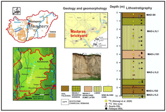
Figure 1.
Location, lithostratigraphy of the studied loess/paleosol sequence of Madaras brickyard with sampling points for 14C [5] AMS, quartz OSL and polymineral pIRIRSL marked.
3. Materials and Methods
3.1. 14C Dating
One charcoal and 30 gastropod shell samples, plus one soil organic matter sample, were collected from the northern part of the loess wall for radiocarbon dating. Figure 1 and Table 1 both present the exact stratigraphic locations of the samples. We used published protocols for sample preparation and measurement [10,11,12]. Samples were pretreated by weak acid (2% HCl) before graphitization to remove surficial contamination and carbonate coatings.

Table 1.
List of samples with conventional and calibrated 14C dates with new unpublished data highlighted.
Radiocarbon dating was undertaken using accelerator mass spectrometry (AMS) at the AMS laboratory of Seattle, WA, USA (Lab code: D-AMS), and Institute for Nuclear Research of the Hungarian Academy of Sciences at Debrecen (Lab code: DeA-) (Table 1). The charcoal sample was measured in the Isotoptech Lab, Debrecen, using conventional counting [10]. Conventional radiocarbon dates were converted to calendar ages using the software Bacon [13] and the most recent IntCal20 calibration curve [14]. Calibrated dates are reported at the 2-sigma confidence level (95.4%).
We consider the resulting 14C dates to be reliable. Certain herbivorous gastropods are known to yield reliable ages for 14C dating since they yield minimal shell age offsets, on the scale of a couple of decades, so allowing construction of highly reliable millennial and even centennial scale age models [15,16,17,18,19,20]. We nevertheless undertook further testing for possible age offset biases attributable to the use of different gastropod taxa by analyzing multiple samples dating from the same depths in the middle and lower parts of the profile (Table 1).
3.2. Luminescence Dating
3.2.1. Sampling and Sample Preparation
Sampling for luminescence dating was undertaken on the cleaned and logged profile (Figure 1). Sampling depths and dosimetry information are given in Table 2 and Table 3 and Figure 1. Metal tubes were driven into the profile to obtain samples for equivalent dose (De) determination, while extra material was taken in watertight pots for analysis of dose rates and water content. Carbonates and organic matter were removed from the De fractions (0.1 M HCl and 15% H2O2), followed by separation of the polymineral 4–11 mm fraction. A fraction of this was immersed in H2SiF6 for two weeks to isolate quartz for optically stimulated luminescence (OSL) dating, followed by a final wash in 0.1 M HCl [21] with the remainder retained for polymineral post-infrared infrared stimulated luminescence dating (pIR-IRSL). OSL infrared (IR) depletion ratios [22] were used to determine the purity of quartz samples. Any sample differing from unity by >10% was retreated via H2SiF6 immersion for a further week. To test the ability of the quartz OSL and pIRIR50,290 to accurately measure laboratory doses given before any laboratory heat treatment, a dose recovery test was performed.
Table 2.
Equivalent doses, dose rates and quartz luminescence ages.
Table 3.
Equivalent doses, dose rates and feldspar luminescence ages.
3.2.2. Quartz OSL
De values were obtained using a modified SAR protocol [23,24] performed on Risø TL-DA-15 TL/OSL reader systems. Samples were measured using a blue LED (λ = 470 ± 20 nm) stimulation source (40 s, c. 39 mW cm−2) and the OSL signal was measured in the UV range using a 9235QA photomultiplier filtered by 6 mm of Hoya U340 [25]. The signal was integrated from the first 0.8 s of stimulation minus a background estimated from the last 8 s. For the quartz measurements, we used the protocol of Stevens et al. [26], followed by an extra IRSL stimulation at room temperature for 40 s prior to each OSL measurement to eliminate contribution from any IR sensitive quartz grains [27,28]. Aliquots yielding recycling ratios [23] or IR depletion ratios [22] differing from unity by greater than 10% were rejected. The uncertainty on individual De values was estimated using Monte Carlo simulation and a weighted mean De (with one standard error uncertainty) was calculated. Dose-response curves were fitted using saturating exponential (single), or saturating exponential plus linear functions in Analyst [29].
3.2.3. Polymineral pIR-IRSL
Post-IR IRSL measurements followed a modified SAR protocol [24,30] performed on Risø TL-DA-15 TL/OSL reader systems. Samples were measured using an infrared LED (λ = 875 nm) stimulation source (200 s, c. 135 mW cm−2) at both 50 °C and 290 °C, with an initial preheat of 320 °C for 60 s. Following the administration of a test dose (30 Gy), these measurements were repeated and followed by an IRSL stimulation at 325 °C for 200 s to remove residual charge [24,30]. Post-IR IRSL 290 °C and 50 °C signals were used for De estimates [24]. Luminescence was detected in the blue-violet region through a Schott BG39 and Corning 7–59 filter combination. The signal was integrated from the first 3.9 s of stimulation minus a background estimated from the last 78 s. Aliquots yielding recycling ratios [23] differing from unity by greater than 10% were rejected. The uncertainty on individual De values was estimated using Monte Carlo simulation and a weighted mean De (with one standard error uncertainty) was calculated for each sample. Dose-response curves were fitted using saturating exponential (single) or saturating exponential plus linear functions in Analyst [29]. Laboratory fading rates were measured for some samples.
3.2.4. Dosimetry
Dose rates were calculated from uranium, thorium, and potassium concentrations measured using Inductively Coupled Plasma Mass Spectrometry (ICP-MS) and Atomic Emission Spectrometry (ICP-AES). Water contents were estimated from the measurements of current values. Alpha efficiency values of 0.04 ± 0.02 (quartz) and 0.08 ± 0.02 (polymineral) were used for dose rate calculation [31]. Alpha and beta attenuation were obtained using calculations in Bell [32] and dose rate conversion factors were taken from published values [33,34,35].
Unknown uncertainties are taken as 10% for all measured quantities. Uncertainties due to beta source calibration (3%) [36], radioisotope concentration (10%), dose rate conversion factors (3%), and attenuation factors (3%) have also been calculated [37]. The cosmic dose calculations used modern burial depth [38]. Dosimetry, De, and age data are presented in Table 2 and Table 3, respectively.
3.3. Age-Depth Modeling
Bayesian modeling using only 14C ages was performed by the software package Bacon [19]. Inverse accumulation rates (sedimentation rates expressed as year/cm) were estimated from 42 to 48 million Markov Chain Monte Carlo (MCMC) iterations, and these rates form the age-depth model. Accumulation rate (AR) was the first constraint using default prior information: acc. shape = 1.5 and acc. mean = 10 for the beta distribution, a memory mean = 0.7 and memory strength = 4 for beta distribution describing the autocorrelation of inverse AR. All input data were provided as 14C yr BP and the model used the northern hemisphere IntCal20 calibration curve [20] to convert conventional radiocarbon ages to calendar ages expressed as cal BP. Age modeling was run to achieve a 5 cm final resolution. Boundary conditions were added based on the observed major lithostratigraphic boundaries at the level of the modern soil (1.5 m), the lowermost pedocomplex (8–9 m). The fit of posterior gamma and beta distributions as well as the 95% CI ranges, plus inverse AR with 95% CI ranges were considered for comparing results of the new model with that of Sümegi et al. [5]. All data and figures are presented in calendar ages expressed as cal BP.
3.4. Sedimentation Rates
Sedimentation times (years/cm) were estimated by MCMC iterations using the acc.rate depth ghost and acc.rate age ghost functions of Bacon. This function allows us to capture variability in accumulation rates and assigned varying uncertainties with depth in contrast to the traditionally applied equation based on mean model ages of consecutive depths and depth intervals yielding sub-optimal results [39].
4. Results and Discussion
4.1. 14C Age Models
Conventional radiocarbon ages deriving from Sümegi et al. [5] and this study are presented in Table 1, now converted using the Intcal20 calibration curve [20]. The new calibration now places the age of the bedrock sand to 39,843 ± 602 cal BP years as opposed to the old one of 39,181 ± 630 cal BP years. The top of the profile at 16 cm has also been slightly modified thanks to the new calibration from 12,856 ± 156 cal BP years to 12,914 ± 164 cal BP years.
Comparing ages yielded by different gastropod taxa for the same horizons at depths of 548–552 cm and 748–752 cm, the following conclusions can be made (Figure 2). Differences in mean ages for the examined taxa of Trochulus hispidus, Granaria frumentum, and Chondrula tridens is negligible both for the conventional (65 and 41 years) and calibrated ages (72 and 54 years). So, any of these gastropods yield suitable results for tackling even centennial-scale changes. Age differences are also minimal between the charcoal and soil organic matter for the same depth interval of 900–904 cm, corresponding to a part of the lowermost paleosol (38 and 106 years, respectively). However, these samples yielded significantly older dates than the bracketing gastropod samples with deviations of 419, 484 years in conventional and 390, and 419 years in calibrated ages, while the difference between the bracketing gastropod samples is minimal (ca. 100 years). Charcoal ages are strongly biased by the ages of the trees, while soil organic matter is also strongly vegetation related. Soil OM ages include the mean residence time of organic C, which can be hundreds or even thousands of years, but they also do not date sedimentation but are best seen as a maximum or minimum age for sedimentation of loess above or below, respectively. The observable internal consistency of the chronology relying on a large gastropod shell 14C age dataset support our idea of using shell ages to date loess accumulation at higher temporal resolution.
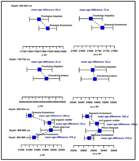
Figure 2.
Comparison of conventional and calibrated ages of different mollusk taxa for samples at the same depths.
The average 95% confidence range for Model 1 in the earlier published chronology [5] was 762 years, with a minimum of 356 years at 400 cm and a maximum of 1628 years at 980 cm. In all, 92% of the dates overlapped with the model’s boundaries. The prior accumulation rates set to 16 years/cm are in good agreement with the calculated whole section average sedimentation time of 16.8 years/cm (15–18 yr/cm 95% CI) [5] (Figure 3). In our revised model with the additional dates (Model 2), the mean 95% confidence range has been significantly reduced to 439 years with a minimum of 169 years at the depth of 903 cm and a maximum of 874 years at 16 cm; 89% of the dates overlap with the model’s ranges. The a priori sedimentation times set for Model 2 was significantly lower (10 years/cm) than that of [5], which used half the number of dates than we provide in our study. The actual whole section average sedimentation time of the new model is 12.09 years/cm (9.5–14.72 yr/cm 95% CI). These values are relevant for the entire profile.
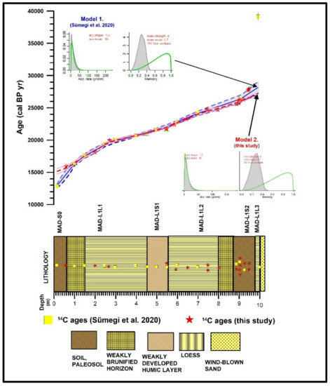
Figure 3.
Comparison of constructed age-depth models of Sümegi et al. (2020) [5] (Model 1) and this study (Model 2) (squares and stars represent mean values of 14C dated horizons included in the model, solid lines represent mean values, dotted lines and whiskers correspond to 95% confidence intervals).
We note that both models neglected the lowermost oldest date of 39,843 ± 302 cal BP years, derived from the aeolian sand (Table 1, Figure 3). We assume that loess accumulation started much later than the deposition of the basal sand. Model 1 [5] placed the start of loess accumulation at 28,119 ± 861 cal BP, while our study placed this datum at 26,994 ± 323 cal BP (Table S1). Model 1 dated the top of the profile to 12,943 ± 263 cal BP [5], whereas we placed it at 15,163 ± 437 cal BP because the latter neglected the topmost calibrated date at the depth of 16 cm. The average 2σ error of 381 ± 176 years for Model 1 has now been reduced to 219 ± 85 years (Table S1). Similarly, the average 95% confidence interval (CI) ranges of 761 ± 352 years (Model 1) have now been reduced to 438 ± 169 years. The average difference between the mean ages of the models is −54 years with a minimum of −1125 years at the base and a maximum of 2220 years at the top of the profile (Table S1). The largest differences in both mean ages and 2σ errors between the two models are confined to the topmost and lowermost pedogenic horizons (Figure 4). Due to the neglect of the last calibrated date at 16 cm depth, Model 2 overestimated the mean ages of Model 1 by ca. 500–2300 years in the upper 1.6 m of the sequence. It is worth noting though that the 2 σ errors have been almost halved from the original 700 years to 250–500 years. In the lowermost ca. 2 m of the sequence, our Model 2 yields younger modelled ages than Model 1 by ca. 500–1300 years (Figure 4), and significantly reduced 2σ errors of 100–300 years. For the rest of the sequence, mean ages of the two models vary within the range of 100–150 years and 2σ errors have been reduced to 200–300 years.
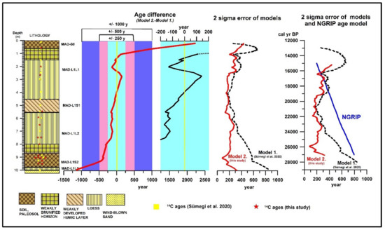
Figure 4.
Observed differences in mean ages as well as 2-sigma uncertainties of Model 1 and 2 as well as uncertainty of the NGRIP age model (14C ages from [5]).
Thus, by doubling the number of dates we have significantly improved the precision of the age model; we have halved the uncertainty values and tightened the 95% CI ranges. Our uncertainties are significantly lower than those of the NGRIP age model from the Greenland ice core [40,41]. The resulting resolution of the Madaras record therefore enables us to investigate potential leads and lags between the terrestrial (loess) and ice records on millennial and centennial timescale (Figure 4).
When comparing our modeled ages with the calibrated ages of the dated depth horizons, we observe a similar pattern (Table S2). The average sampled depth interval was 32 cm, with a minimum of 2 cm and a maximum of 1 m. Leaving out the topmost (16 cm) and lowermost (998 cm) dated horizons, the average time span of the sampled intervals was 380 years with a minimum of 2 and a maximum of 1085 years. In general, where sampling intervals were around 50 cm or less, the represented age span between the sampled intervals is below 500 years. The largest period of ca. 1000 years between two sampled depth horizons are generally confined to large sampling intervals of ca. 1 m. Looking at the general pattern we can expect a reduction by half if additional dated depths are introduced at 50 cm intervals. However, since the 2 σ errors of our model remains broadly consistent throughout the entire profile (Figure 4), we can expect minimal reduction in model uncertainties by increasing the density of dated intervals.
4.2. Quartz OSL and Polymineral pIRIRSL Data
In general, the average water content of the samples was relatively high (29.93 ± 1.19%) (Table S5), compared to other MIS 2 luminescence records from the Carpathian Basin [42,43,44]. Preheat plateaus were observed from 220 °C up to 260 °C for quartz (Figure 5A) and 100 °C to 250 °C for polymineral fine samples (Figure 5B). Measured-to-given dose ratios for quartz were 0.87 ± 0.12 (n = 2 sample), 0.8 ± 0.11 (n = 2 sample) for post-IR IRSL50, and 0.97 ± 0.13 (n =2 sample) for post-IR IRSL290, respectively, confirming the suitability of the measurement protocol (Figure 6).
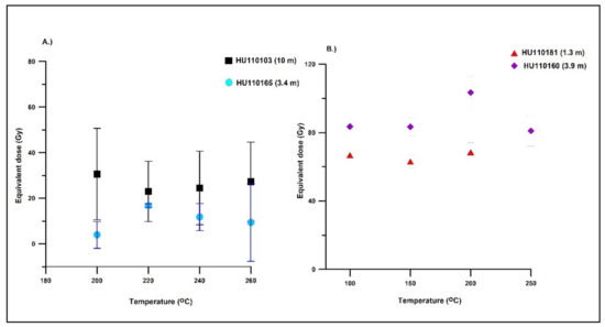
Figure 5.
Results of preheat plateau tests for selected quartz (A) and feldspar (B) samples.
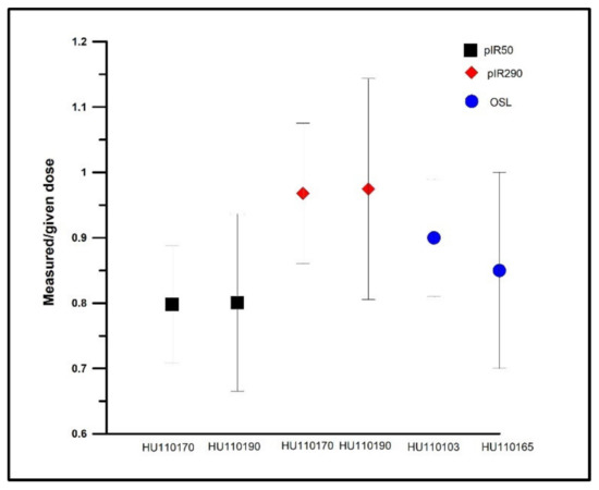
Figure 6.
Ratio of measured/recovered dose rates for selected quartz and feldspar samples.
The uranium, thorium, and potassium contents range from 1.5 ± 0.05 to 2.8 ± 0.08 ppm, 6.5 ± 0.20 to 10.2 ± 0.31 ppm and 0.94 ± 0.00 to 1.61 ± 0.01 %, respectively (Table S5). The total dose rate for quartz ranges from 2.17 ± 0.11 to 2.90 ± 0.16 Gy ka−1 (Table 2, Figure S1), which is slightly below the ones for some nearby Serbian sites (3.09 ± 0.18 Gy ka−1, 3.22 ± 0.18 Gy ka−1 [45], but close to the value of some Hungarian sites (Paks: 2.33–2.48 ± 0.10 Gy ka−1 [46], Süttő: 1.62 + −0.11 – 2.14 + −0.15 [47]). The total dose rate for feldspars ranges from 2.13 ± 0.09 to 3.35 ± 0.16 Gy ka−1, which is slightly below the values for most samples from the Danube catchment Serbian [30,45,48,49,50], Romanian [51,52,53], Austrian [54], Croatian [55,56,57,58], and Hungarian samples [15,46,47]. Calculated dose rates for feldspars (mean: 2.78 ± 0.13 Gy ka−1) and quartz (mean: 2.39 ± 0.08 Gy ka−1) follow an upward decreasing trend with minor fluctuations (Figure S1).
Quartz OSL ages date the base sands to 28.16 ± 1.8 ka; the top of the profile dates to the Middle Holocene (4.61 ± 0.54 to 2.17 ± 0.63 ka) (Table 2). Looking at the OSL ages, there are major inversions upwards in the profile starting in the paleosol overlying the base sands (HU110103, 6.64 ± 1.88 ka). Quartz OSL measurements yielded extremely young ages (5.98 ± 0.93 ka to 7.59 ± 1.34 ka) at depths between 670–520 cm (Table 2).
The unexpectedly young ages require some interrogation as to the reason for the discrepancy from the radiocarbon chronology. In the case of the sample HU110103 from 1000 cm depth (6.64 ± 1.88 ka), measured total dose rates are normal. All measured aliquots display rapidly decaying OSL signals indicating that they are dominated by the fast OSL component (Figure 7). It is worth noting, however, that approximately two thirds of the measured aliquots (7/24) were rejected due to poor recycling ratios (Table 2). On Figure 7, displaying decay and dose response curves of selected aliquots for sample HU110103 (1000 cm), only a single aliquot had a De value of 52.77 ± 13 Gy consistent with the stratigraphy. The remaining six aliquots had very low De values (15.86 ± 2.65 Gy to 25.54 ± 5.96 Gy). In the overlying sample (HU110119, 840 cm) De values are higher with an average of 58.01 ± 15.13 Gy, again consistent with the stratigraphy (Table 2), yet only three of the six aliquots yielded acceptable De values due to poor recycling. In the case of the samples (HU110135, HU110139, HU110147) with anomalously young ages between 670–520 cm depths, a large proportion of aliquots were also rejected due to poor recycling (Table 2). The only exception is sample HU110147 at the depth of 520 cm, where 10 of the 15 aliquots were acceptable. For sample HU110139 at the depth of 610 cm, only a single aliquot yielded acceptable but very low De value (14.39 ± 1.63 Gy). When we look at the dose response curves of the referenced samples, all display a rapid decay (Figures S3–S5) but signals are extremely dim. In the case of the sample HU110165 at the depth of 340 cm, only ca. half of the measured aliquots were accepted (Table 2), which may have led to age underestimation (De: 33.73 ± 8.83 Gy) compared to the overlying sample at 300 cm (HU110169 De: 54.33 ± 9.9 Gy) where five of the six aliquots yielded acceptable De values. Decay curves of both samples again are dominated by the fast component (Figures S6 and S7). In general, all samples display rapidly decaying OSL signals indicating that they are dominated by the fast OSL component. In samples where a large portion of aliquots yielded acceptable De values, we generally find De values consistent with the stratigraphy. In the samples of low signal, a large proportion of the aliquots had to be refused due to poor recycling and sometimes poor recuperation values. When we compare the quartz OSL ages with 14C ages of the same depth in the intervals characterized by low De values, OSL ages are ca. 10–17 ky younger than corresponding 14C dates from the same level (Table S3, Figure 8). The only reasonably acceptable ages are confined to depths of 300, 840 cm (Table S3, Figure 8).
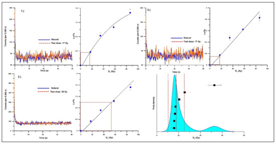
Figure 7.
Dose response and decay curves obtained for given (1), (2) and (3) different aliquots of quartz sample HU110103 at the depth of 1000 cm.
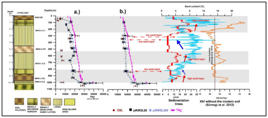
Figure 8.
Comparison of 14C based chronology with quartz OSL, feldspar pIRIRSL ages as well a sand content, sediment accumulation rates derived from 14C age-depth models and magnetic susceptibility values (a) all luminescence data included, (b) filtered-note gray bands mark zones of reduced accumulation and increased pedogenesis (Xhf data from [6]).
Feldspar pIRIRSL ages presented in Table 3 are not corrected for fading, since the fading calculated for some samples was minimal (0.65–1%/Gy). The received ages are more consistent with the documented chronostratigraphy of the LPS [5] than the quartz OSL ages. Here, pIRIRSL50 measurements dated the base sand between 42 and 30 ka (Table 3, Figure 8), and the topmost part is placed to the Holocene (11–5 ka). There is an inversion at the depth of 90 cm to an age dated to the Late Glacial (16 ka). However, these measurements significantly underestimated the 14C modeled ages for the remaining major part of the LPS (−5.078 ky on average with a minimum of −10.4 ky and maximum of 320 y) (Table S4) and several horizons are characterized by significant inversions (Figure 8). The smallest differences between 14C and pIRIRSL50 ages are noted at the depth of 540 and 90 cm (−1273 and 320 years), and both of these horizons show significant inversion in ages compared to the underlying horizons.
pIRIRSL290 measurements placed the age of the base sands between 37 and 30 ka (Table 3, Figure 8). These ages are generally consistent with both pIRIRSL50 and the unmodeled 14C ages of the base sand. The start of loess accumulation is put to ca. 27 ka by both methods, which are also consistent with the modeled 14C ages. pIRIRSL290 dates show an upward decrease again but with major inversions at certain horizons (Table 3, Figure 8) and underestimate the 14C modeled ages in general (by 4.8 ky on average) (Table S4). The smallest differences between 14C and pIRIRSL290 ages are observed at the depths of 540 and 90 cm (−1306 and 78 years). Differences between pIRIRSL50 and pIRIRSL290 ages are minimal (a couple of hundred years) in general (Table S4). When looking at the pIRIRSL dose response curves of samples for various depth intervals all samples all aliquots yielded fairly consistent De values with minimal scatter compared to quartz OSL results (Figures S8–S10).
Summarizing the luminescence data, quartz samples exhibit very dim signals with poor recycling and sometimes recuperation ratios that led to a lot of rejected aliquots; together, this might be responsible for the observed age inversions throughout the profile and the large age underestimations in comparison to the radiocarbon ages. Therefore, we do not regard these age data reliable without further detailed methodological investigations. The pIRIRSL data scatter less, but the ages still show some age inversions; some samples underestimate the radiocarbon data significantly, while others agree within their respective uncertainty. Interestingly, the age inversions are observed in horizons with decreased sediment accumulation (see below). As the age inversions are not really understood at this point, we regard the luminescence data in general as preliminary and requiring further study.
4.3. Sedimentation Rates Compared between the Two Models and Other Coeval MIS 2 Sites of the Carpathian Basin
We observe higher mean sedimentation times for the entire sequence compared with the previously published value (12.07 ± 2.65 yr/cm compared with 16.8 yr/cm (15–18 yr/cm 95% CI). Our calculations are based on mid-point estimates calculated for 1 cm intervals using double the number of dates. This rate is higher, but very close to, the one published for Dunaszekcső (13.3 yr/cm) [4]. As noted in Sümegi et al. [5], the data for Dunaszekcső was inferred from the total thickness of the LPS and bracketing calibrated 14C ages. We confirmed this by running a model for the published data [4] and calculated the sedimentation time to 15.8 yr/cm [5]. This value is closer to the one published for Madaras by Sümegi et al. [5], although the two sequences are only partially overlapping in time (Dunaszekcső bw. 36–23.4 ky cal BP and Madaras 27–15 ky cal BP). It is also worth emphasizing that the accumulation rates span the entire LPSs. Based on this data, the 2 and 4 cm sampling intervals at Madaras correspond to 24 ± 5.3 and 48 ± 10.6 years, respectively.
Sedimentation times calculated for the Madaras LPS show a close correspondence with measured magnetic susceptibility values published in Sümegi et al. [6] (Figure 9), with high values corresponding to pedogenized horizons and loess yielding low values. There is an upward increasing rate of accumulation from ca. 5 m to 2.5 m accompanied by a similar decreasing trend in magnetic susceptibility. The slowest accumulation is generally confined to the base and modern paleosols. Based on the reduced accumulation rates and higher magnetic susceptibility values (Figure 8 and Figure 9) between 540 and 690 cm, the discrepancy with the visually observed lithostratigraphic position of the middle weakly developed humic layer-placed between 450 and 550 cm on the lithological column, may require further explanation. Here, we also observe increased sedimentation times with values (15 y/cm) similar to the base soil MAD L1S2 (920–950 cm). The unique patterning seen in the mentioned interval of 540 and 690 cm is an artefact of upbuilding pedogenesis due to constant and strong dust input to the area marked by the proximity of values close to the inferred loess base line (Figure 8, [6]). In this horizon, we can also see a high sand input to the site as depicted on Figure 8. A similarly higher input of sand was notable in the lowermost base soil MAD L1S2 (920–950 cm), as depicted on Figure 8. In the mentioned intervals (540 and 690 cm and 920–950 cm), the MS signal moves closer to the loess base line of Sümegi et al. (2012) [6], parallel with the upward increase in the sand input again confirming the idea of upbuilding pedogenesis in these horizons.
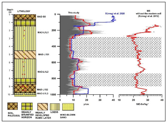
Figure 9.
Sedimentation times (inverse AR in y/cm) calculated for 14C Model 1 (Sümegi et al., 2020) [5] and Model 2 (this study) and magnetic susceptibility data from Sümegi et al. (2012) [6]. Note: solid lines on sedimentation times correspond to average model values, gray shading represents 95% CI of the models, gray bands depict areas of reduced sedimentation times and parallel decreasing trend in and/or reduced magnetic susceptibility values.
Sedimentation times for the time interval representing MIS 2 (bw 28 and 21 ky) are highly variable across the Carpathian Basin (Table 4): Krems (14.5 yr/cm–4.7 m) [42], Süttő (18.3 yr/cm–3.45 m) [47] Tokaj (12.2 yr/cm–4.6 m) [43], Dunaszekcső (11.7 yr/cm–4.36 m) [4], Titel (17.2 yr/cm–2.4 m) [44], Surduk 2 (54.5 yr/cm–1.54 m) [59] and Madaras (11.6 yr/cm–4.87 m [5]; 10.8 yr/cm–5.56 m-this study). These variable accumulation rates are partly attributable to actual variations throughout MIS 2. In some records (e.g., Titel, Dunaszekcső), only a part of the entire period representing MIS 2 was preserved. In addition, sedimentation times in all but two records (Madaras, Dunaszekcső) were calculated using simple interpolation between depth intervals corresponding to MIS 2, ignoring variation in sedimentation. The mean sedimentation time of the Madaras LPS calculated from the Bayesian age-depth model (10.78 ± 2.34 years/cm) is the highest so far recorded in the Carpathian Basin for MIS 2. Temporal variations in most of the listed profiles are much less resolved yielding uniform accumulation rates for longer periods due to the low number of dates available. The two exceptions are the Dunaszekcső and Madaras profiles, where a sufficient density of dated horizons renders the tackling of centennial-scale variations in accumulation rates possible. As the Dunaszekcső profile covers only a part of the LGM (ca. 2600 years), the so far best resolved LGM sequence of the Carpathian Basin is given by the Madaras LPS.
Table 4.
Comparison of sedimentation times for various MIS 2 Carpathian Basin profiles.
5. Conclusions
A twofold increase in the density of sampling for 14C dating significantly reduces uncertainties in the age-depth model at Madaras LPS. The low 2σ uncertainties of our new model remain relatively constant throughout the entire profile. This relative consistency in the 14C shell dates based on a large dataset corroborates the accuracy of the new 14C based chronology. It would appear that 0.5 m sampling intervals represent the optimal density of sampling; adding more dates may not actually improve precision of the model significantly. Since our 2 σ uncertainties are significantly lower than those of the NGRIP age model [40,41], our model is suitable for making direct correlations at high temporal resolution.
We observe that pIRIRSL ages, though clearly underestimating by a couple of hundred years, show very good agreement with 14C ages in general (Figure 8b). An almost perfect agreement is notable at the depths of 100 and 1000 cm. The inversions in both pIRIRSL ages are synchronous and generally appear in horizons (1000–800 cm, 730–540 cm, 250–0 cm) where accumulation slows down (Figure 8). These are marked by the gray bands in Figure 9. By contrast, we observe significant age underestimation and poor signal behavior in the quartz OSL ages compared to both pIRIRSL and 14C ages. These, however, also seem to be confined to areas where accumulation slows down similarly to pIRIRSL ages, as depicted by the gray bands on Figure 8 mentioned previously. OSL ages appear to be consistent with 14C ages at three depths alone (300, 850, 1050 cm, Figure 8b). It is interesting to note that despite the general upward increase, the sand content seems to be anticorrelated with the accumulation rates. When sediment accumulation drops, the sand content increases, and vice versa. In general, we observe poor signal behavior and age discrepancies in the sandier horizons with higher accumulation rates. This pattern appears to be systematic for all OSL and pIRIRSL ages. Luminescence dating does not encounter such problems in loess areas with much higher sand content than the Madaras LPS, such as the Holocene loesses of the Great Plains (USA) [60,61], which could reflect differences in the sources of the sand. Dim signals and wide distributions in quartz De values, especially for different grain-size samples, have been reported in several studies [51,52,53,62], although whether the observed differences relate to intrinsic properties of the quartz or bleaching remains as yet unexplained. Several studies are known to establish a link between luminescence characteristics and provenance [61], as well as geochemical composition [46,63,64,65,66]. Several studies suggest the addition of non-sensitized quartz grains from freshly eroded, proximal source rocks to be the cause of unusual quartz signal behavior [67,68], particularly where there has been an influx of sand to loess sediments. The proximity of sand dunes to the Madaras site may evoke the same explanation for our study site (Figure 10).
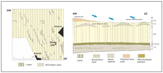
Figure 10.
Surface geology and idealized sketch of the Late Pleistocene geohistory of the Hungarian part of the Bácska loess area (adopted from Molnár and Krolopp [73]).
Several studies have dealt with the geology of the Hungarian part of the Bácska Loess Plateau, down to a depth of ca. 30 m [5,6,69,70,71,72,73,74]. On the northern part, at a depth of 30 m, the bedrock is given by loess overlain by wind-blown sands in 5 to 10 m thickness. The wind-blown sands are followed by a three-membered loess horizon divided by wind-blown sand layers of 1 to 3 m thickness [69,70,71,72,73,74]. The same can be expected to the southern part as well, where our study site is located, with the exception of the reduced role of interbedded sand layers [73]. Figure 10 adopted from Molnár and Krolopp [73] presents an idealized sketch of the Late Pleistocene geohistory of the Bácska Loess Area, using a NW-SE cross-section. At the base there is a thin layer of wind-blown sand, sometimes with an intercalation of a thin loess layer overlain by a paleosol horizon [5,6,73]. This is topped by typical loess in 6 to 10 m thickness. The one-time loess surface was often blanketed by wind-blown sand transported to the area from the nearby dunes by the predominant winds from the NW during warmer, drier interstadials. This wind-blown sand appears in most cases in the form of lens or minor buried dunes. However, the material is not pure sand but represent transitions from sand to loess (sandy loess-loessy sand). Where the loess overlying it and of later origin was removed by erosion, the sandy loess or loessy sand hummocks might have been exposed from time to time, acting as nearby sources of sand (Figure 10). So, there is every reason to believe that the addition of non-sensitized quartz grains to our deposits during these periods from smaller, proximal source rocks and areas might have played a significant role in signal loss [67,68]. This is in line with our observations that the horizons with abrupt, unusual quartz signal shifts are all characterized by a drop in accumulation and a higher sand input, the latter most likely deriving from nearby re-exposed sand dunes (Figure 9). The exceptional thickness of the Madaras profile compared to other coeval LPS of the Bácska loess plateau, with a more southerly position [44,59], must be attributed to the proximity of the source areas, too. Further corroboration may come from complex provenience studies like Fenn et al. [75].
The geochronological data on the quartz from the Madaras loess section of the study area may be supported by the fact that the study area is related to Danube former alluvium [73]; the low sensitivity of the quartz is not only limited to the upper (Alpine) part of the Danube catchment [75,76,77,78], but can be detected in the downstream region, and clearly characterizes Danube River-related fluvial and translocated sediments [79]. All grain sizes studied in the region appear to be characterized by low luminescence sensitivity in quartz [79]. The Madaras section appears to be typical for the Danube alluvial fan area, for which much of its sediment originated from the Alps [73], and which is likely to have influenced the luminescence behavior of the quartz at a catchment scale. The low sensitivity values, which negatively affected OSL measurements and age data, have been demonstrated throughout our study area, the Danube alluvial fan [79], and as a consequence, thousands of years of differences have been detected in geochronological measurements [80].
Supplementary Materials
The following supporting information can be downloaded at: https://www.mdpi.com/article/10.3390/quat5040047/s1. Figure S1. Quartz, feldspar dose rates within the studied LPS. Figure S2. Dose response and decay curves obtained for different aliquots of quartz sample HU110119 at the depth of 840 cm. Figure S3. Dose response and decay curves obtained for different aliquots of quartz sample HU110135 at the depth of 670 cm. Figure S4. Dose response and decay curves obtained for different aliquots of quartz sample HU110139 at the depth of 610 cm. Figure S5. Dose response and decay curves obtained for different aliquots of quartz sample HU110147 at the depth of 520 cm. Figure S6. Dose response and decay curves obtained for different aliquots of quartz sample HU110165 at the depth of 340 cm. Figure S7. Dose response and decay curves obtained for different aliquots of quartz sample HU110169 at the depth of 300 cm. Figure S8. Dose response and decay curves obtained for different aliquots of polymineral pIRIRSL290 samples I. Figure S9. Dose response and decay curves obtained for different aliquots of polymineral pIRIRSL290 samples II. Figure S10. Dose response and decay curves obtained for different aliquots of polymineral pIRIRSL290 samples III. Table S1. Age differences between modelled dates of Sümegi et al. (2020) (Model 1) and the present study (Model 2). Table S2. Calibrated and modelled ages and calculated per sample age-depth intervals. Table S3. Comparison of 14C and quartz OSL dates. Table S4. Comparison of 14C, feldspar pIRIRSL50 and pIRIRSL290 dates. Table S5. Water contents, radionuclide contents relevant to OSL and IRSL ages.
Author Contributions
Conceptualization, P.S., S.G., D.M., K.F. and T.S.; methodology, P.S., S.G., T.S. and K.F.; software, D.M., L.M., and P.C.; validation, P.S., S.G., T.S. and K.F.; formal analysis, K.F., J.J.N. and F.L.; investigation, D.M., L.M., P.C., D.H. and M.M.; resources, P.S. and F.L.; data curation, P.S. and S.G.; writing—review and editing, P.S., S.G.,D.H. and K.F.; visualization, S.G., L.M. and P.C.; supervision, P.S., T.S., and K.F.; project administration, P.S. and D.M.; funding acquisition, P.S. and M.M. All authors have read and agreed to the published version of the manuscript.
Funding
This research was funded by the Hungarian Ministry of Human Capacities, grant number: 20391-3/2018/FEKUSTRAT, and the European Regional Development Fund, grant number: GINOP-2.3.2-15-2016-00009 ‘ICER’.
Data Availability Statement
The data presented in this study are available on request from the corresponding author.
Conflicts of Interest
The authors declare no conflict of interest.
References
- Muhs, D.R.; Bettis, E.A. Quaternary loess-Paleosol sequences as examples of climate-driven sedimentary extremes. Geological Society of America Special Paper 370. Extrem. Depos. Environ. Mega End Memb. Geol. Time 2003, 70, 53–74. [Google Scholar] [CrossRef]
- Obreht, I.; Zeeden, C.; Hambach, U.; Veres, D.; Marković, S.B.; Lehmkuhl, F. A critical reevaluation of palaeoclimate proxy records from loess in the Carpathian Basin. Earth-Sci. Rev. 2019, 190, 498–520. [Google Scholar] [CrossRef]
- Rousseau, D.-D.; Boers, N.; Sima, A.; Svensson, A.M.; Bigler, M.; Lagroix, F.; Taylor, S.M.; Antoine, P. MIS3 & 2 millennial oscillations in Greenland dust and Eurasian aeolian records—A paleosol perspective. Quat. Sci. Rev. 2017, 169, 99–113. [Google Scholar]
- Újvári, G.; Stevens, T.; Molnár, M.; Demény, A.; Lambert, F.; Varga, G.; Timothy, A.J.; Páll-Gergely, B.; Buylaert, J.P.; Kovács, J. Coupled European and Greenland last glacial dust activity driven by North Atlantic climate. Proc. Natl. Acad. Sci. USA 2017, 114, 10632–10638. [Google Scholar] [CrossRef] [PubMed]
- Sümegi, P.; Gulyás, S.; Molnár, D.; Szilágyi, G.; Sümegi, B.; Törőcsik, T.; Molnár, M. 14C Dated Chronology of the Thickest and Best Resolved Loess/Paleosol Record of the LGM from SE Hungary Based on Comparing Precision and Accuracy of Age-Depth Models. Radiocarbon 2020, 62, 403–417. [Google Scholar] [CrossRef]
- Sümegi, P.; Gulyás, S.; Csökmei, B.; Molnár, D.; Hambach, U.; Stevens, T.; Markovic, S.; Almond, P. Climatic fluctuations inferred for the Middle and Late Pleniglacial (MIS 2) based on high-resolution (ca 20yr) preliminary environmental magnetic investigation of the loess section of the Madaras brickyard. Cent. Eur. Geol. 2012, 55, 329–345. [Google Scholar] [CrossRef]
- Bokhorst, M.P.; Vandenberghe, J.; Sümegi, P.; Lanczont, M.; Gerasimenko, N.P.; Matviishina, Z.N.; Markovic, S.B.; Frechen, M. Atmospheric circulation patterns in central and eastern Europe during the Weichselian Pleniglacial inferred from loess grain-size records. Quat. Int. 2011, 234, 64–72. [Google Scholar] [CrossRef]
- Hupuczi, J.; Sümegi, P. The Late Pleistocene paleoenvironment and paleoclimate of the Madaras section (South Hungary), based on preliminary records from mollusks. Cent. Eur. J. Geosci. 2010, 2, 64–70. [Google Scholar] [CrossRef]
- Sümegi, P. Loess and Upper Paleolithic Environment in Hungary; Aurea Kiadó: Nagykovácsi, Hungary, 2005. [Google Scholar]
- Hertelendi, E.; Csongor, É.; Záborszky, L.; Molnár, I.; Gál, I.; Győrffy, M.; Nagy, S. Counting system for high precision C-14 dating. Radiocarbon 1989, 32, 399–408. [Google Scholar] [CrossRef]
- Hertelendi, E.; Sümegi, P.; Szöőr, G. Geochronologic and paleoclimatic characterization of Quaternary sediments in the Great Hungarian Plain. Radiocarbon 1992, 34, 833–839. [Google Scholar] [CrossRef]
- Molnár, M.; Janovics, R.; Major, I.; Orsovszki, J.; Gönczi, R.; Veres, M.; Leonard, A.G.; Castle, S.M.; Lange, T.E.; Wacker, L.; et al. Status Report of the New AMS 14C Sample Preparation Lab of the Hertelendi Laboratory of Environmental Studies (Debrecen, Hungary). Radiocarbon 2013, 55, 665–676. [Google Scholar] [CrossRef]
- Blaauw, M.; Christen, J.A. Flexible paleoclimate age-depth models using an autoregressive gamma process. Bayesian Anal. 2011, 3, 457–474. [Google Scholar] [CrossRef]
- Reimer, P.; Austin, W.; Bard, E.; Bayliss, A.; Blackwell, P.G.; Ramsey, C.B.; Butzin, M.; Cheng, H.; Edwards, R.L.; Friedrich, M. TheIntCal20 Northern Hemisphere radiocarbon age calibration curve (0–55 cal kBP). Radiocarbon 2020, 62, 725–757. [Google Scholar] [CrossRef]
- Pigati, J.S.; Quade, J.; Shanahan, T.M.; Haynes, C.V., Jr. Radiocarbon dating of minute gastropods and new constraints on the timing of spring-discharge deposits in southern Arizona, USA. Palaeogeogr. Palaeoclimatol. Palaeoecol. 2004, 204, 33–45. [Google Scholar] [CrossRef]
- Pigati, J.S.; Rech, J.A.; Nekola, J.C. Radiocarbon dating of small terrestrial gastropod shells in North America. Quat. Geochronol. 2010, 5, 519–532. [Google Scholar] [CrossRef]
- Pigati, J.S.; McGeehin, J.P.; Muhs, D.R.; Bettis, E.A., III. Radiocarbon dating late Quaternary loess deposits using small terrestrial gastropod shells. Quat. Sci. Rev. 2013, 76, 114–128. [Google Scholar] [CrossRef]
- Sümegi, P.; Hertelendi, E. Reconstruction of microenvironmental changes in Kopasz Hill loess area at Tokaj (Hungary) between 15,000–70,000 BP years. Radiocarbon 1998, 40, 855–863. [Google Scholar] [CrossRef]
- Újvári, G.; Molnár, M.; Novothny, Á.; Páll-Gergely, B.; Kovács, J.; Várhegyi, A. AMS 14C and OSL/IRSL dating of the Dunaszekcső loess sequence (Hungary): Chronology for 20 to 150 ka and implications for establishing reliable age-depth models for the last 40 ka. Quat. Sci. Rev. 2014, 106, 140–154. [Google Scholar] [CrossRef]
- Xu, B.; Gu, Z.; Han, J.; Hao, Q.; Lu, Y.; Wang, L.; Wu, N.; Peng, Y. Radiocarbon age anomalies of land snail shells in the Chinese Loess Plateau. Quat. Geochronol. 2011, 6, 383–389. [Google Scholar] [CrossRef]
- Berger, G.W.; Mulhern, P.J.; Huntley, P.J. Isolation of silt-sized quartz from sediments. Anc. TL 1980, 11, 8–9. [Google Scholar]
- Duller, G.A.T. Distinguishing quartz and feldspar in single grain luminescence measurements. Radiat. Meas. 2003, 37, 161–165. [Google Scholar] [CrossRef]
- Murray, A.S.; Wintle, A.G. Luminescence dating of quartz using an improved single-aliquot regenerative-dose procedure. Radiat. Meas. 2000, 32, 57–73. [Google Scholar] [CrossRef]
- Murray, A.S.; Wintle, A.G. The single-aliquot regenerative dose protocol: Potential improvements in reliability. Radiat. Meas. 2003, 37, 377–381. [Google Scholar] [CrossRef]
- Bøtter-Jensen, L.; Andersen, C.E.; Duller, G.A.T.; Murray, A.S. Developments in radiation, stimulation and observation facilities in luminescence measurements. Radiat. Meas. 2003, 37, 535–541. [Google Scholar] [CrossRef]
- Stevens, T.; Armitage, S.J.; Lu, H.; Thomas, D.S.G. Examining the potential of high sampling resolution OSL dating of Chinese loess. Quat. Geochronol. 2007, 2, 15–22. [Google Scholar] [CrossRef]
- Banerjee, D.; Murray, A.S.; Bøtter-Jensen, L.; Lang, A. Equivalent dose determination from a single aliquot of polymineral fine grains. Radiat. Meas. 2001, 33, 73–94. [Google Scholar] [CrossRef]
- Wang, X.; Lu, Y.; Zhao, H. On the performances of the single-aliquot regenerative-dose (SAR) protocol for Chinese loess: Fine quartz and polymineral grains. Radiat. Meas. 2006, 41, 1–8. [Google Scholar] [CrossRef]
- Duller, G.A.T. Assessing the error on equivalent dose estimates derived from single aliquot regenerative dose measurements. Anc. TL 2007, 25, 15–24. [Google Scholar]
- Stevens, T.; Markovic, S.B.; Zech, M.; Hambach, U.; Sümegi, P. Dust deposition and climate in the Carpathian Basin over an independently dated last glacial-interglacial cycle. Quat. Sci. Rev. 2011, 30, 662–681. [Google Scholar] [CrossRef]
- Rees-Jones, J. Optical dating of young sediments using fine-grain quartz. Anc. TL 1995, 13, 9–13. [Google Scholar]
- Bell, W.T. Alpha dose attenuation in quartz grains for thermoluminescence dating. Anc. TL 1980, 12, 4–8. [Google Scholar]
- Adamiec, G.; Aitken, M.J. Dose rate conversion factors: Update. Anc. TL 1998, 16, 37–50. [Google Scholar]
- Liritzis, I.; Stamoulis, K.; Papachristodoulou, C.; Ioannides, K. A re-evaluation of radiation dose-rate conversion factors. Mediterr. Archaeol. Archaeom. 2013, 13, 1–15. [Google Scholar]
- Guerin, G.; Mercier, N.; Adamiec, G. Dose-rate conversion factors: Update. Anc. TL 2011, 29, 5–8. [Google Scholar]
- Armitage, S.J.; Bailey, R.M. The measured dependence of laboratory beta dose rates on sample grain size. Radiat. Meas. 2005, 39, 123–127. [Google Scholar] [CrossRef]
- Murray, A.S.; Olley, J.M. Precision and accuracy in the optically stimulated luminescence dating of sedimentary quartz: A status review. Geochronometria 2002, 21, 1–16. [Google Scholar]
- Prescott, J.R.; Hutton, J.T. Cosmic ray contributions to dose rates for luminescence and ESR dating: Large depths and long-term variations. Radiat. Meas. 1994, 23, 497–500. [Google Scholar] [CrossRef]
- Blaauw, M.; Christen, J.A.; Benett, K.D.; Reimer, P.J. Double the dates and go for Bayes-Impacts of model choice, dating density and quality of chronologies. Quat. Sci. Rev. 2018, 188, 58–66. [Google Scholar] [CrossRef]
- North Greenland Ice-Core Project (NGRIP) Members. High resolution record of Northern Hemisphere climate extending to the Last Interglacial period. Nature 2004, 431, 147–151. [Google Scholar] [CrossRef]
- Rasmussen, S.O.; Andersen, K.K.; Svensson, A.M.; Steffensen, J.P.; Vinther, B.M.; Clausen, H.B.; Siggaard-Andersen, S.J.; Larsen, L.B.; Dahl-Jensen, D.; Bigler, M.; et al. A new Greenland ice core chronology for the last glacial termination. J. Geophys. Res. Atmos. 2006, 111, D06102. [Google Scholar] [CrossRef]
- Lomax, J.; Fuchs, M.; Preusser, F.; Fiebig, M. Luminescence based loess chronostratigraphy of the Upper Palaeolithic site Krems-Wachtberg, Austria. Quat. Int. 2014, 351, 88–97. [Google Scholar] [CrossRef]
- Schatz, A.K.; Buylaert, J.P.; Murray, A.; Stevens, T.; Scholten, T. Establishing a luminescence chronology for a palaeosol-loess profile at Tokaj (Hungary): A comparison of quartz OSL and polymineral IRSL signals. Quat. Geochronol. 2012, 10, 68–74. [Google Scholar] [CrossRef]
- Perić, Z.; Lagerbäck, A.E.; Stevens, T.; Újvári, G.; Zeeden, C.; Buylaert, J.P.; Marković, S.B.; Hambach, U.; Fischer, P.; Schmidt, C.; et al. Quartz OSL dating of late quaternary Chinese and Serbian loess: A cross Eurasian comparison of dust mass accumulation rates. Quat. Int. 2019, 502, 30–44. [Google Scholar] [CrossRef]
- Murray, A.S.; Schmidt, E.D.; Stevens, T.; Buylaert, J.P.; Marković, S.B.; Tsukamoto, S.; Frechen, M. Dating Middle Pleistocene loess from Stari Slankamen (Vojvodina, Serbia)—Limitations imposed by the saturation behaviour of an elevated temperature IRSL signal. Catena 2014, 117, 34–42. [Google Scholar] [CrossRef]
- Thiel, C.; Horváth, E.; Frechen, M. Revisiting the loess/palaeosol sequence in Paks, Hungary: A post-IR IRSL based chronology for the ‘Young Loess Series’. Quat. Int. 2014, 319, 88–98. [Google Scholar] [CrossRef]
- Novothny, Á.; Frechen, M.; Horváth, E.; Wacha, L.; Rolf, C. Investigating the penultimate and last glacial cycles of the Süttő loess section (Hungary) using luminescence dating, high-resolution grain size, and magnetic susceptibility data. Quat. Int. 2011, 234, 75–85. [Google Scholar] [CrossRef]
- Schmidt, E.D.; Machalett, B.; Marković, S.B.; Tsukamoto, S.; Frechen, M. Luminescence chronology of the upper part of the Stari Slankamen loess sequence (Vojvodina, Serbia). Quat. Geochr. 2010, 5, 137–142. [Google Scholar] [CrossRef]
- Perić, Z.M.; Marković, S.B.; Sipos, G.; Gavrilov, M.B.; Thiel, C.; Zeeden, C.; Murray, A.S. A post-IR IRSL chronology and dust mass accumulation rates of the Nosak loess-palaeosol sequence in northeastern Serbia. Boreas 2020, 49, 841–857. [Google Scholar] [CrossRef]
- Marković, S.B.; Vandenberghe, J.; Stevens, T.; Mihailović, D.; Gavrilov, M.B.; Radaković, M.G.; Zeeden, C.; Obrecht, I.; Perić, Z.M.; Nett, J.J.; et al. Geomorphological evolution of the Petrovaradin Fortress Palaeolithic site (Novi Sad, Serbia). Quat. Res. 2021, 103, 21–34. [Google Scholar] [CrossRef]
- Constantin, D.; Begy, R.; Vasiliniuc, S.; Panaiotu, C.; Necula, C.; Codrea, V.; Timar-Gabor, A. High-resolution OSL dating of the Costinesti section (Dobrogea, SE Romania) using fine and coarse quartz. Quat. Int. 2014, 334–335, 20–29. [Google Scholar] [CrossRef]
- Timar, A.; Vandenberghe, D.; Panaiotu, E.C.; Panaiotu, C.G.; Necula, C.; Cosma, C.; Vanden haute, P. Optical dating of Romanian loess using fine-grained quartz. Quat. Geochronol. 2010, 5, 143–148. [Google Scholar] [CrossRef]
- Timar, A.; Vandenberghe, D.A.G.; Vasiliniuc, S.; Panaoitu, C.E.; Panaoitu, C.G.; Dimofte, D.; Cosma, C. Optical dating of Romanian loess: A comparison between silt-sized and sand-sized quartz. Quat. Int. 2011, 240, 62–70. [Google Scholar] [CrossRef]
- Thiel, C.; Buylaert, J.P.; Murray, A.; Terhost, B.; Hofer, I.; Tsukamoto, S.; Frechen, M. Luminescence dating of the Stratzing loess profile (Austria)—Testing the potential of an elevated temperature post-IR IRSL protocol. Quat. Int. 2011, 234, 23–31. [Google Scholar] [CrossRef]
- Wacha, L.; Frechen, M. The geochronology of the “Gorjanović loess section” in Vukovar, Croatia. Quat. Int. 2011, 240, 87–99. [Google Scholar] [CrossRef]
- Wacha, L.; Vlahović, I.; Tsukamoto, S.; Kovačić, M.; Hasan, O.; Pavelić, D. The chronostratigraphy of the latest Middle Pleistocene aeolian and alluvial activity on the Island of Hvar, eastern Adriatic, Croatia. Boreas 2015, 45, 152–164. [Google Scholar] [CrossRef]
- Wacha, L.; Rolf, C.; Hambach, U.; Frechen, M.; Galović, L.; Duchoslav, M. The Last Glacial aeolian record of the Island of Susak (Croatia) as seen from a high-resolution grain–size and rock magnetic analysis. Quat. Int. 2018, 494, 211–224. [Google Scholar] [CrossRef]
- Wacha, L.; Laag, C.; Grizelj, A.; Tsukamoto, S.; Zeeden, C.; Ivanisević, D.; Rolf, C.; Banak, A.; Frechen, M. High-resolution palaeoenvironmental reconstruction at Zmajevac (Croatia) over the last three glacial/interglacial cycles. Paleog. Paleoc. Paleoe. 2021, 546, 110504. [Google Scholar] [CrossRef]
- Fenn, K.; Durcan, J.A.; Thomas, D.S.G.; Millar, I.L.; Markovic, S.B. Re-analysis of late Quaternary dust mass accumulation rates in Serbia using new luminescence chronology for loess–palaeosol sequence at Surduk. Boreas 2020, 49, 634–652. [Google Scholar] [CrossRef]
- Miao, X.; Hanson, R.; Stohr, C.J.; Wang, H. Holocene loess in Illinois revealed by OSL dating: Implications for stratigraphy and geoarcheology of the Midwest United States. Quat. Sci. Rev. 2018, 200, 253–261. [Google Scholar] [CrossRef]
- Tecsa, V.; Mason, J.A.; Johnson, W.C.; Miao, X.; Constantin, D.; Radu, S.; Magdas, D.A.; Veres, D.; Markovic, S.B.; Timar-Gabor, A. Latest Pleistocene to Holocene loess in the central Great Plains: Optically stimulated luminescence dating and multi-proxy analysis of the enders loess section (Nebraska, USA). Quat. Sci. Rev. 2020, 229, 106130. [Google Scholar] [CrossRef]
- Nett, J.J.; Chu, W.; Fischer, P.; Hambach, U.; Klasen, N.; Zeeden, C.; Obreht, I.; Obrocki, L.; Pötter, S.; Gavrilov, M.B.; et al. The Early Upper Paleolithic Site Crvenka-At, Serbia–The First Aurignacian Lowland Occupation Site in the Southern Carpathian Basin. Front. Earth Sci. 2021, 9, 56. [Google Scholar] [CrossRef]
- Gray, H.J.; Jain, M.; Sawakuchi, A.O.; Mahan, S.A.; Tucker, G.E. Luminescence as a sediment tracer and provenance tool. Rev. Geophys. 2019, 57, 987–1017. [Google Scholar] [CrossRef]
- Götte, T.; Ramseyer, K. Trace element characteristics, luminescence properties and real structure of quartz. In Quartz: Deposits, Mineralogy and Analytics; Götze, J., Möckel, R., Eds.; Springer: Berlin/Heidelberg, Germany, 2012; pp. 265–285. [Google Scholar]
- Stevens, T.; Adamiec, G.; Bird, A.F.; Lu, H. An abrupt shift in dust source on the Chinese Loess Plateau revealed through high sampling resolution OSL dating. Quat. Sci. Rev. 2013, 82, 121–132. [Google Scholar] [CrossRef]
- Rodrigues, A.L.; Dias, M.I.; Valera, A.C.; Rocha, F.; Prudencio, M.I.; Marques, R. Geochemistry, luminescence and innovative dose rate determination of a Chalcolithic calcite-rich negative feature. J. Archaeol. Sci. Rep. 2019, 26, 101887. [Google Scholar] [CrossRef]
- Pietsch, T.J.; Olley, J.M.; Nanson, G.C. Fluvial transport as a natural luminescence 20eli20tizer of quartz. Quat. Geochronol. 2008, 3, 365–376. [Google Scholar] [CrossRef]
- Fitzsimmons, K.E. Anassessment of the luminescence sensitivity of Australian quartz with respect to sediment history. Geochronometria 2011, 38, 199–208. [Google Scholar] [CrossRef]
- Miháltz, I. A Duna-Tisza köze déli részének Földtani felvétele (Geological survey of the southern part of the Danube-Tisza Interfluve). Magy. Állami Földtani Intézet Jelentése Az 1950-Es Évről 1953, 1, 113–144. (In Hungarian) [Google Scholar]
- Molnár, B. Die Verbreitung der aeolischen bildungen an der oberflache und untertags im Zwischenstromland von Donau und Theiss. Földtani Közlöny 1961, 91, 300–315. (In German) [Google Scholar]
- Molnár, B. Pliocene and Pleistocene lithofacies of the Great Hungarian Plain. Acta Geol. Hung. 1970, 14, 445–457. [Google Scholar]
- Molnár, B. A Duna-Tisza köze felső-pliocén és pleisztocén fejlődéstörténete (Upper Pliocene and Pleistocene geohistory of the Danube-Tisza Interfluve). Földtani Közlöny 1975, 107, 1–16. (In Hungarian) [Google Scholar]
- Molnár, B.; Krolopp, E. Latest Pleistocene geohistory of the Bácska Loess Area. Acta Min. Petro. 1978, 23, 245–265. [Google Scholar]
- Molnár, B. Quaternary geohistory of the Hungarian part of the Danube-Tisza Interfluve. Proc. Geol. Inst. Belgrade 1988, 21, 61–78. [Google Scholar]
- Fenn, K.; Thomas, D.S.G.; Durcan, J.A.; Millar, I.L.; Veres, D.; Piermattei, A.; Lane, C.S. A tale of two signals: Global and local influences on the Late Pleistocene loess sequences in Bulgarian Lower Danube. Quat. Sci. Rev. 2021, 274, 107264. [Google Scholar] [CrossRef]
- Moska, P.; Murray, A.S. Stability of the quartz fast-component in insensitive samples. Radiat. Meas. 2006, 41, 878–885. [Google Scholar] [CrossRef]
- Klasen, N.; Fiebig, M.; Preusser, F.; Radtke, U. Luminescence properties of glaicofluvial sediments from Bavarian Alpine Foreland. Radiat. Meas. 2006, 41, 866–870. [Google Scholar] [CrossRef]
- Klasen, N.; Fiebig, M.; Preusser, F.; Reiner, J.M.; Radtke, U. Luminescence dating of proglacial sediments from the Eastern Alps. Quat. Int. 2007, 164–165, 21–32. [Google Scholar] [CrossRef]
- Tóth, O.; Sipos, G.; Kiss, T.; Bartyik, T. Variation of OSL residual doses in terms of coarse and fine grain modern sediments along the Hungarian section of the Danube. Geochronometria 2017, 44, 319–330. [Google Scholar] [CrossRef]
- Tóth, O.; Sipos, G.; Kiss, T.; Bartyik, T. Dating the Holocene incision of the Danube in Southern Hungary. J. Environ. Geogr. 2017, 10, 53–59. [Google Scholar] [CrossRef][Green Version]
Publisher’s Note: MDPI stays neutral with regard to jurisdictional claims in published maps and institutional affiliations. |
© 2022 by the authors. Licensee MDPI, Basel, Switzerland. This article is an open access article distributed under the terms and conditions of the Creative Commons Attribution (CC BY) license (https://creativecommons.org/licenses/by/4.0/).