Article

Erosion Risk Assessment for Prioritization of Conservation Measures in the Watershed of Genale Dawa-3 Hydropower Dam, Ethiopia

1
Department of Hydraulic and Water Resources Engineering, Bule Hora University (BHU), Bule Hora 144, Ethiopia
2
Department of Hydraulic and Water Resources Engineering, Hawassa University Institute of Technology (HUIoT), Hawassa 05, Ethiopia
*
Author to whom correspondence should be addressed.
Quaternary 2022, 5(4), 39; https://doi.org/10.3390/quat5040039
Submission received: 16 August 2022 / Revised: 6 September 2022 / Accepted: 9 September 2022 / Published: 23 September 2022

Abstract

:
Sedimentation is a leading global problem that affects the environment and dams by reducing the live storage capacity of reservoirs and the life expectance of dams. Hence, prioritizing watersheds according to the risk of soil loss is crucial for extending the useful life of dams and reservoirs. The objectives of this study were to assess sediment flow in the Genale Dawa-3 reservoir, identify subbasins that are prone to soil erosion, and evaluate the impact of different management practices on minimizing sediment yields by using the Soil and Water Assessment Tool (SWAT) model. The SWAT model was calibrated and validated by observed streamflow and sediment data based on the SUFI-2 algorithm by SWAT-CUP, and its performance was assessed. The model simulated the average annual sediment yield; the input to the reservoir was 16.83 ton/ha/yr for the period of 1990–2015. From a total of 31 subbasins, 12 were categorized from high to very severe (11–60 ton/ha/yr) sediment-yielding subbasins and selected for sediment management. The simulated scenarios showed that the average annual sediment reductions at critical erosion hot spots in subbasins after the application of filter strips, soil/stone bund, terracing, and contour farming were 35.03%, 66.54%, 80.88%, and 53.11%, respectively. Therefore, this study concluded that reducing sediment yield by implementing terracing in critical areas at risk of soil erosion was more effective than other soil conservation measures. Overall, this research can help planners and decision-makers to implement appropriate soil conservation measures in the most erosive subwatersheds in order to extend the useful life of the Genale Dawa-3 hydropower dam and reservoir.

1. Introduction

Soil erosion is a major environmental issue on a global scale. It reduces water quality and soil productivity, increases sediments in reservoirs, and increases the likelihood of flooding [1]. According to [2], around 40,000 large reservoirs are impacted by siltation worldwide, and it is expected that 0.5 to 1 percent of the total storage capacity is lost annually. Nowadays, the problem is a serious issue all over the world since it drastically diminishes the reservoir’s original capacity, which has an impact on recreational, hydropower, and drinking water supplies as well as flood control and agriculture [3]. Due to a lack of reservoir sediment management practices, such as periodic sediment flushing, reservoir sediment routing, and planned catchment management activities, reservoir sedimentation is an increasing problem for many nations [3,4]. By reducing the original capacity of reservoirs, sedimentation results in the unstable operation of many dams [5].
As reported by [6,7,8,9,10,11], the effects of sedimentation are serious for developing countries such as Ethiopia. In Ethiopia, sediment deposition in reservoirs is threatening the sustainability of dams built for various purposes [12,13]. The reservoir sediment survey done by [13] in Ethiopia indicated that only 30% of the reservoirs were expected to last for their entire design period. Another 50% of the studied reservoirs were losing their economic life before half of their design period, and 20% of the reservoirs lost less than half during their design period. Therefore, it is necessary to show the relevance of a sediment management model to water resources projects to alleviate soil erosion and reservoir sedimentation.
The Genale Dawa-3 hydropower project comprises a large roller-compacted concrete dam and an underground powerhouse. The 110 m high dam created a large reservoir with a surface area of 98 km² and a total storage capacity of 2570 million m3. The Genale River is the major source of water for the Genale Dawa-3 dam reservoir, which has a live storage capacity of 2310 million m3. The total installed capacity of the plant is 254 MW. However, the storage volume of this reservoir is threatened by soil erosion and sedimentation from the upstream Genale watershed. A vital element in reservoir design and operation is its sedimentation problem. Sediment delivered to the reservoir comes from two principal sources: first, the river feeding the reservoir and second, the valleys on each facets of the reservoir [14]. Hence, an important parameter that reduces the rate of sedimentation of a reservoir is to reduce the sediment yield of the watershed [15]. To do this, it is crucial to evaluate the spatial variations in sediment yield in the watershed and identify key areas that are vulnerable to erosion. Moreover, it is necessary to identify the appropriate best management practices (BMPs) to stop the deterioration of the watershed and reduce sedimentation problems of dams and reservoirs [16,17].
Hence, to manage the sedimentation problems of the Genale Dawa-3 hydropower dam and its watershed, it is necessary to estimate and understand the watershed sediment yield of the basin and identify areas of erosion susceptible parts of the watersheds. Therefore, the main goals of this study were to estimate the sediment yield, identify soil-erosion-susceptible subwatersheds, and evaluate the impact of different BMPs that can aid in the sustainable use of land and water resources in the watershed.

2. Methodology

2.1. Description of the Study Area

2.1.1. Location and Topography

The Genale-Dawa River basin is the 12th drainage basins of Ethiopia and is located in the south-eastern part of the country. It is the third-largest basin in Ethiopia after the Abbay and Wabe Shebele River basin. The basin has a total area of 172,880 km2 or about 15.3% of the total area of Ethiopia. The Genale Dawa-3 scheme is located within the Genale-Dawa River basin, along the middle reach of the Genale River around 655 km from Addis Ababa. The location of the study area lay at latitude 5° 38’ N and longitude 39° 43’ E with a drainage area of 10,264 km2. The description of the study area is shown in (Figure 1).
The altitude of the catchment area ranges from 1039 to 3751 m above sea level (m.a.s.l). The general topographical features of the Genale Dawa-3 dam watershed are highlands and plateaus surrounded by a series of volcanoes, steep slopes, gently sloping lowlands at the foot of the steep slopes, and floodplain areas.

2.1.2. Climate

The entire Genale Dawa-3 dam watershed falls under the bimodal rainfall regime with two wet seasons. The bimodal regime is divided into two types: Type-I, where the rainfall lasts from April to October for around 7 months with less pronounced peaks at the beginning and end, and Type-II, when the rainfall has pronounced peaks in April and October with little rainfall in between these peaks.
Within the study area, the highest annual rainfall corresponds to 1334.61 mm at the Hagerselam station located in the upper region close to the Genale Dawa-3 dam watershed. The lowest annual rainfall corresponds to 633.47 mm at the Negele station located near the outlet of the Genale Dawa-3 dam watershed. As in other parts of the country, the average temperature changes in the Genale Dawa-3 dam watershed are minimal over the long run. The maximum and minimum mean monthly range of temperatures show only a slight change from month to month, with values ranging from 18 °C to 26 °C and 6 °C to 15 °C, respectively. The maximum and minimum mean annual temperatures are 22 °C and 10.5 °C, respectively.

2.1.3. Land Use and Land Cover

The main land use/cover of the Genale Dawa-3 dam watershed is cultivated land, shrub and grassland, forest, developed areas, water, and barren land. In the watershed, the area covered by different land use/cover percentages during 2015 was characterized by 61.11% of cultivated land, 20.68% of shrub and grassland, 14.74% of forestland, 1.68% of built-up area, 1.3% of water body, and 0.48% of barren land. Thus, the land use/cover of the watershed was dominated by cultivated land, shrub, and grassland.

2.1.4. Hydrology

The upper and center parts of the Genale River drains to the GD-3 hydropower site and it has a surface area of 10,264 km2. The upper Genale, Geberticha, and Iya are the three main tributaries that make up the upper section’s main river drainage system. The Sidamo Highlands separate the Genale River basin from the nearby Rift Valley Lake basins and Wabe Shebelle river basins and are the source of these streams. At the location of the dam, the river’s mean annual flow was calculated to be 104.04 m3/s.

2.2. Data Sources

The spatial and temporal data shown in Table 1 were used to create and set up the SWAT model and to simulate the stream and sediment yields of the basin. The model was calibrated and validated using streamflow and sediment data obtained at an inflow gauging (Chenemasa) station. The missing streamflow data from the Chenemasa station were filled by linear regression. The data quality control tests for streamflow were performed by using outlier and homogeneity tests (Pettit test algorithm). The analysis results showed that there was no lower or higher outlier, and the station data were homogeneous.
Similarly, the study area land use/cover data were obtained from Landsat-8 OLI (Operational Land Imager) (Table 1). The satellite images of the watershed with a high resolution and free of cloud cover were downloaded from the US Geological Survey (USGS) (https://earthexplorer.usgs.gov/, accessed on 10 January 2015). A supervised classification method was applied, and its accuracy was assessed. As a result, its overall accuracy was 87.9% with a kappa coefficient of 0.8402.

2.3. Methodology

2.3.1. SWAT Model Description

SWAT is a semidistributed physically based model developed to assess the effects of land management activities on water, sediment, and agricultural chemical yields over extended periods of time in watersheds with a variety of soils, land uses, and management practices [18].
SWAT subdivides a basin into subbasins. Each subbasin is then further subdivided into hydrologic response units (HRUs), which are made up of homogenous land use, management, topographical, and soil features [18]. This partitioning is especially helpful when various basin areas are dominated by land uses or soils that are sufficiently dissimilar to impact the hydrology and can spatially refer to one another [19]. In SWAT, runoff and sediment movements are simulated at the HRU level, and the water and sediment are then routed through the stream network to the basin outlet [19]. The water balance equation (Equation (1)) is used to simulate the hydrological components at each HRU.
S W t =   S W 0   + i = 1 t ( R d a y Q s u r f E a W s e e p Q q w )
where S W t is the final soil water content (mm), R d a y   is the amount of precipitation on day I (mm), S W 0 is the initial soil water content on day i (mm), t is the time (days), E a is the amount of evapotranspiration on day i (mm), Q s u r f is the amount of surface runoff on day i (mm), Q q w is the amount of return flow on day i (mm), and W s e e p is the amount of water entering the vadose zone from the soil profile on day i (mm).
In the watershed, the SWAT model simulates runoff using the curve number approach of the Soil Conservation Services (SCS) [20]. It estimates the surface runoff based on Equation (2).
Q s u r f = ( R d a y I a ) 2 ( R d a y I a + S )
where Q s u r f is the accumulated runoff or rainfall excess (mm), S is the retention parameter (mm), I a is an initial abstraction that includes surface storage, interception, and infiltration before runoff (mm), and R d a y is the rainfall depth for the day (mm). The soils, land use, management, slope, and temporary variations in soil water content all cause the retention parameter to vary geographically. Equation (3) could be used to compute it.
S = 25.4 ( 1000 C N 10 )
where C N is the curve number for the day. The initial abstraction, Ia, is commonly approximated as 0.2 S and Equation (2) becomes:
Q s u r f = ( R d a y 0.2   S ) 2 ( R d a y + 0.8   S )
Using the Modified Universal Soil Loss Equation (MUSLE) [21], the SWAT model calculates the amount of soil erosion and sediment yield caused by water for each HRU. In MUSLE, the delivery ratios are not required, and the equation can be applied to specific storm occurrences since the runoff factor used in USLE in place of the rainfall energy factor improves the prediction of sediment yield. The MUSLE is
S e d = 11.8 ( Q s u r f × q p e a k × A H R U ) 0.56 × K U S L E × C U S L E × P U S L E × L S U S L E × C F R G
where S e d is the sediment amount on a given day in metric tons, Q s u r f is the surface runoff from the catchment in mm/ha, A H R U is the area of HRU, q p e a k is the peak runoff rate in (m3/s), C U S L E is the USLE land cover and management factor, K U S L E is the USLE soil erodibility factor, L S U S L E is the USLE topographic factor, P U S L E is the USLE support practice factor, and C F R G is the coarse fragment factor.
The sediment routing practice, which simulates the movement of sediment through the channel network to the outlet, is made up of two parts: deposition and degradation in the reach [19]. A deposition or degradation process will occur depending on the concentration of sediment in the reach and the transport capacity. Once the deposition and degradation have been estimated, the volume of sediment in the reach could be determined as follows:
S e d c h = s e d c h , i s e d d e p + s e d d e g
where S e d c h is the quantity of suspended sediment in the reach (metric tons), s e d d e p is the quantity of sediment deposited in the reach segment (metric tons), s e d c h , i is the quantity of suspended sediment in the reach at the beginning of the time period (metric tons), and s e d d e g is the quantity of sediment re-entrained in the reach segment (metric tons).
Finally, the amount of sediment moved out of the reach is then determined as:
S e d o u t = s e d c h × V o u t V c h
where S e d o u t is the amount of sediment transported out of the reach (metric tons), V c h is the volume of water in the reach segment (m3), V o u t is the volume of outflow during the time step (m3), and s e d c h is the amount of suspended sediment in the reach (metric tons).

2.3.2. SWAT Model Inputs and Setup

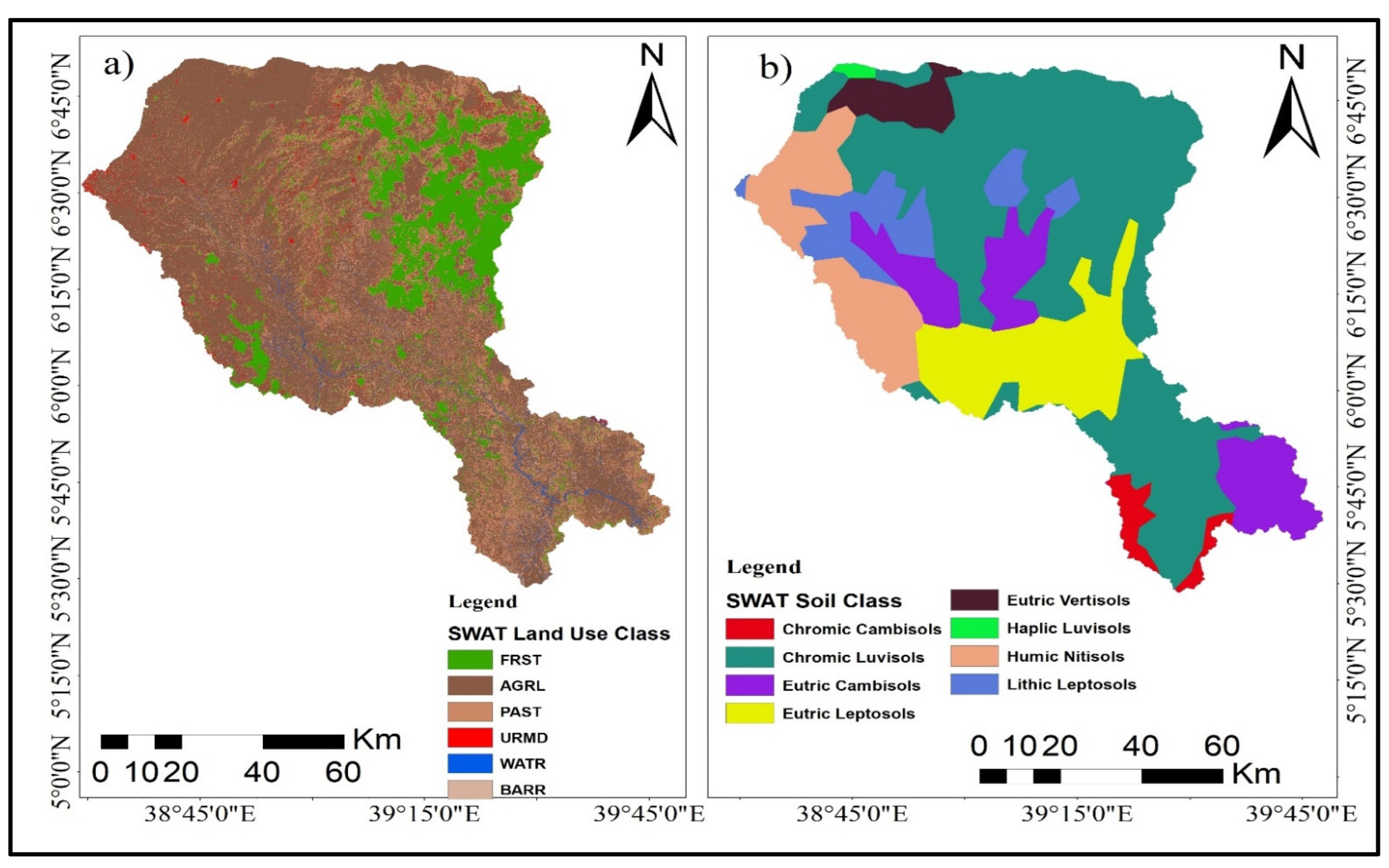
The main input data utilized for the SWAT model involved both spatial and temporal data. The Land use/cover information (Figure 2a), research area’s soil map (Figure 2b), and digital elevation model (DEM) represent the spatial data. The meteorological information, which is used in the simulation, includes precipitation, maximum and lowest temperatures, relative humidity, wind speed, and solar radiation. The weather data used in this study were obtained from five meteorological stations in and around the watershed (Table 2). After collecting the necessary weather data of the representative stations to run the SWAT model, the missing data and data quality control tests were performed. For this study, the missing weather data were filled by using XLSTAT2019 (Excel add-ins) based on the multiple imputation techniques (MCMC), whereas the data quality control tests were made by using a homogeneity test (using Pettis algorithm) and a consistency test (using double-mass curve techniques). The analysis results showed that all selected meteorological stations were homogeneous and consistent. The main purpose of conducting a data quality control test is to minimize the model uncertainty. For this study, the Kibremengist station was the principal (synoptic) station. Thus, this station was used to generate weather data for other stations. The Kibremengist meteorological station has data on the daily duration of sunlight, and Ångström’s empirical formula [
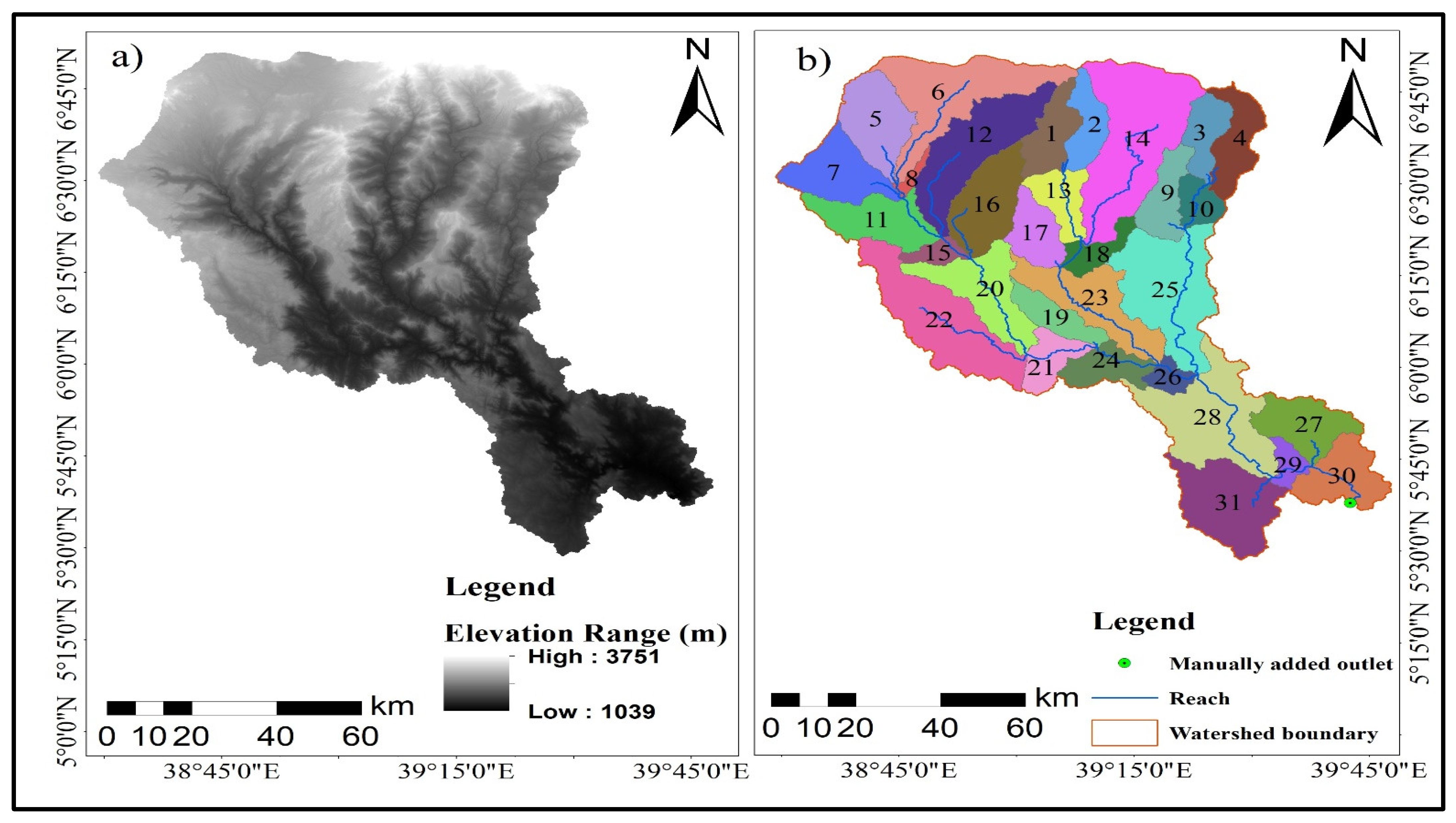
22] was used to convert solar radiation to terrestrial radiation, whereas the duration of relative sunshine was used to estimate the daily solar radiation to be used in the SWAT model. A 30 m × 30 m DEM (Figure 3a) was used to delineate the watershed. Moreover, a threshold area of 17,250 ha was taken, and the entire study area was discretized into 31 subbasins (Figure 3b). Then, the HRUs were defined using a threshold value of 10%, 10%, 15% for land use, soil, and slope, respectively. A total of 253 HRUs were identified, denoting unique combinations of soil type, land use, and slope.

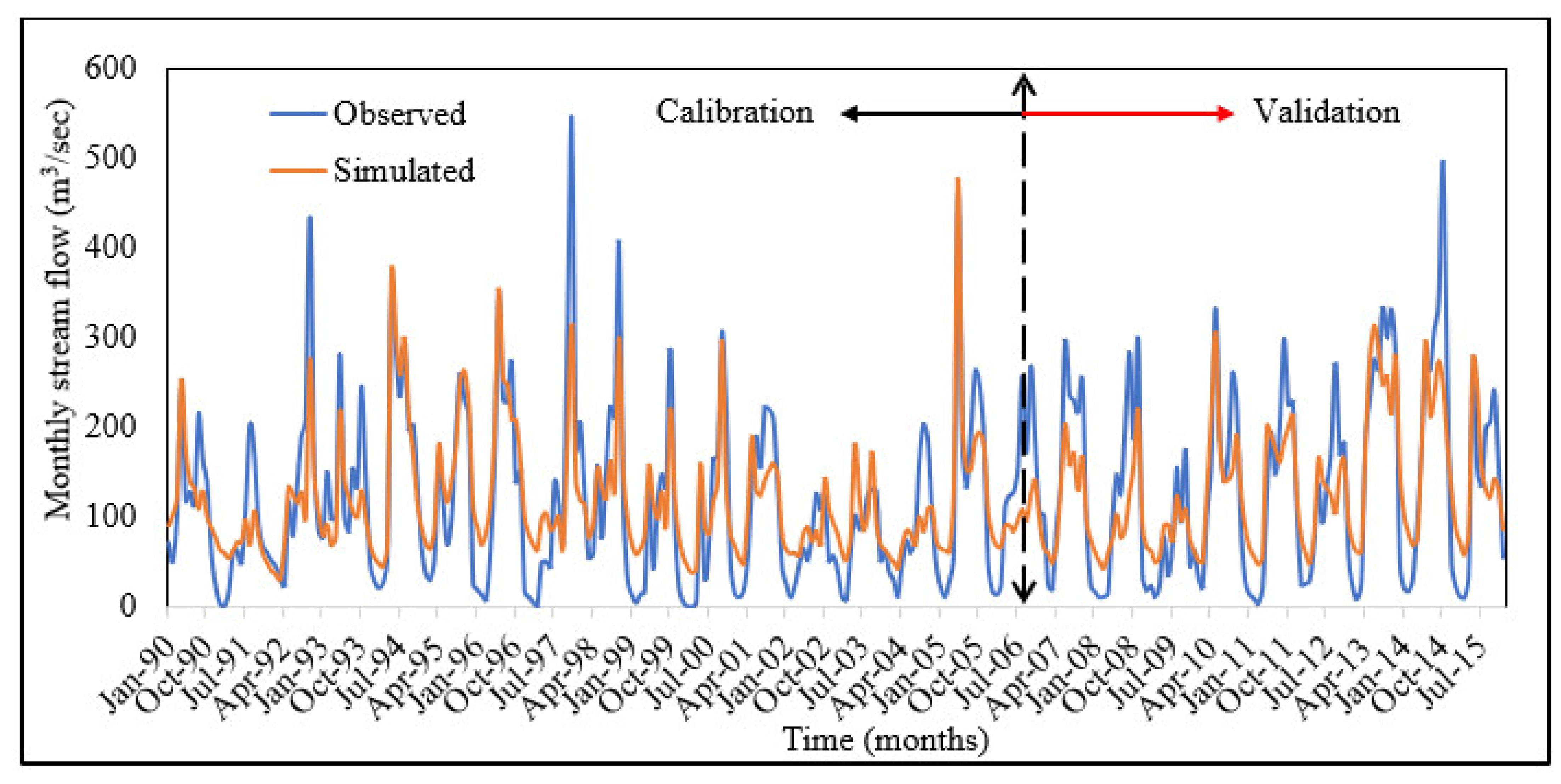
2.3.3. Sensitivity Analysis, Model Calibration, and Validation

SWAT CUP 2019 was used to carry out the streamflow sensitivity analysis and sediment yield analysis for this project. To prioritize the subbasins on the basis of their risk of erosion, the performance of the SWAT model was tested by calibrating and validating the model. To calibrate and obtain the ideal model parameters, the Sequential Uncertainty Fitting (SUFI-2) option was used. After calibration, the model was validated for both stream and sediment flows. The meteorological data from 1987 to 2015 were used in the model simulation. A warm-up period of three years of data was used. The warm-up period is important to make sure that there are no effects from the initial conditions in the model. It enables the hydrologic processes to reach an equilibrium condition and permits the formation of the fundamental flow conditions for the simulations to take place.
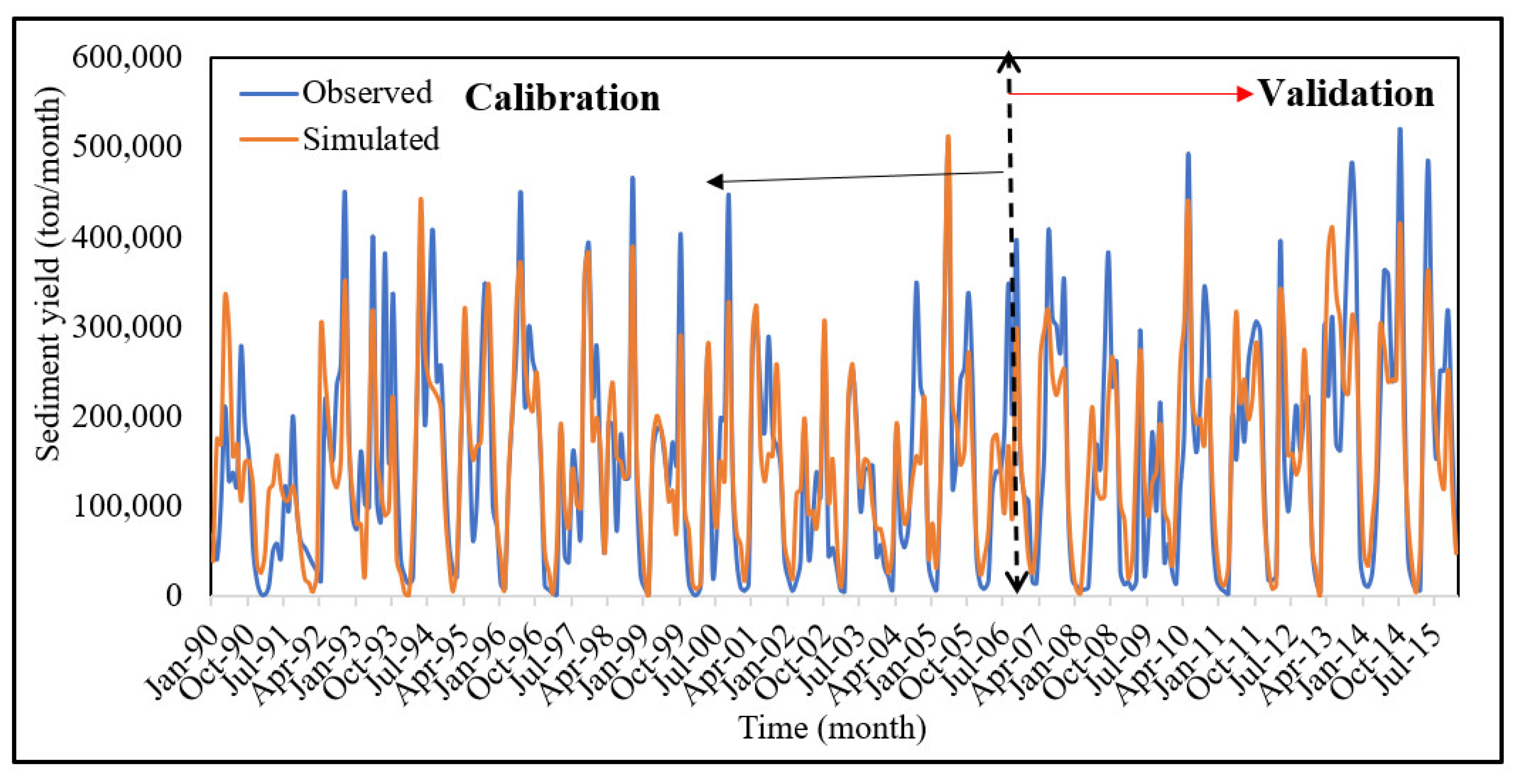
Based on the length of observed stream and sediment flow data records, the calibration and validation periods lengths were fixed. As shown in Table 1, the basin had streamflow data for the years 1990 to 2015. For both stream and sediment flows, the observed datasets were split into two-thirds and one-third to use for calibration and validation, respectively. Based on this, the years from 1990 to 2006 were used for calibration, and 2007 to 2015 were used for validation
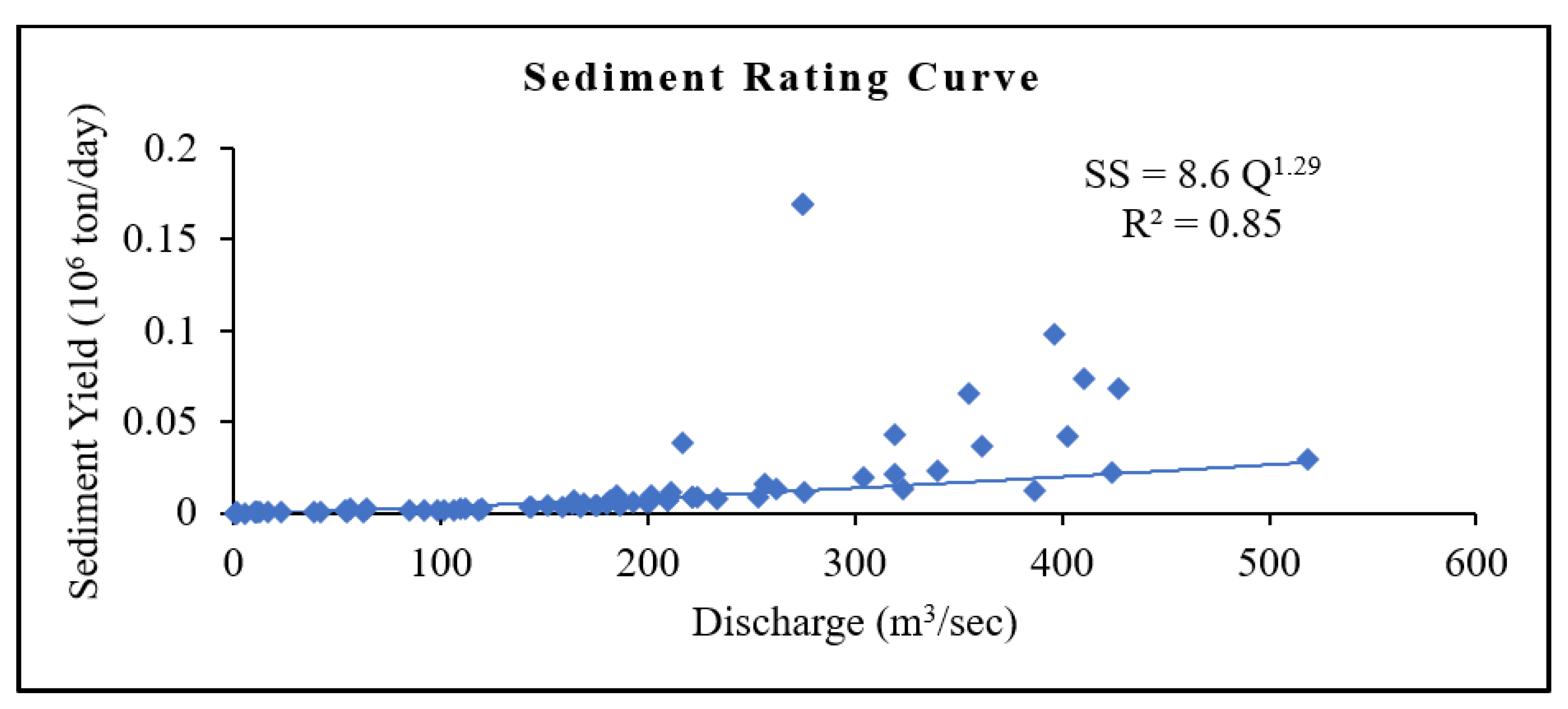
The availability of sediment data was fragmented (Figure 4). Hence, a sediment rating curve was developed and used to convert the sediment flow for the entire period.

2.3.4. Model Performance Evaluation

Statistical measurements were used to assess how well the SWAT model performed.
To evaluate the model’s performance, the Nash–Sutcliffe efficiency (NSE), the percent of bias (PBIAS), the root-mean-square error to observation standard deviation ratio (RSR), and the coefficient of determination (R2) were used. Using the recommendations provided by [23], it was decided whether the model’s performance was sufficient or not (Table 3).

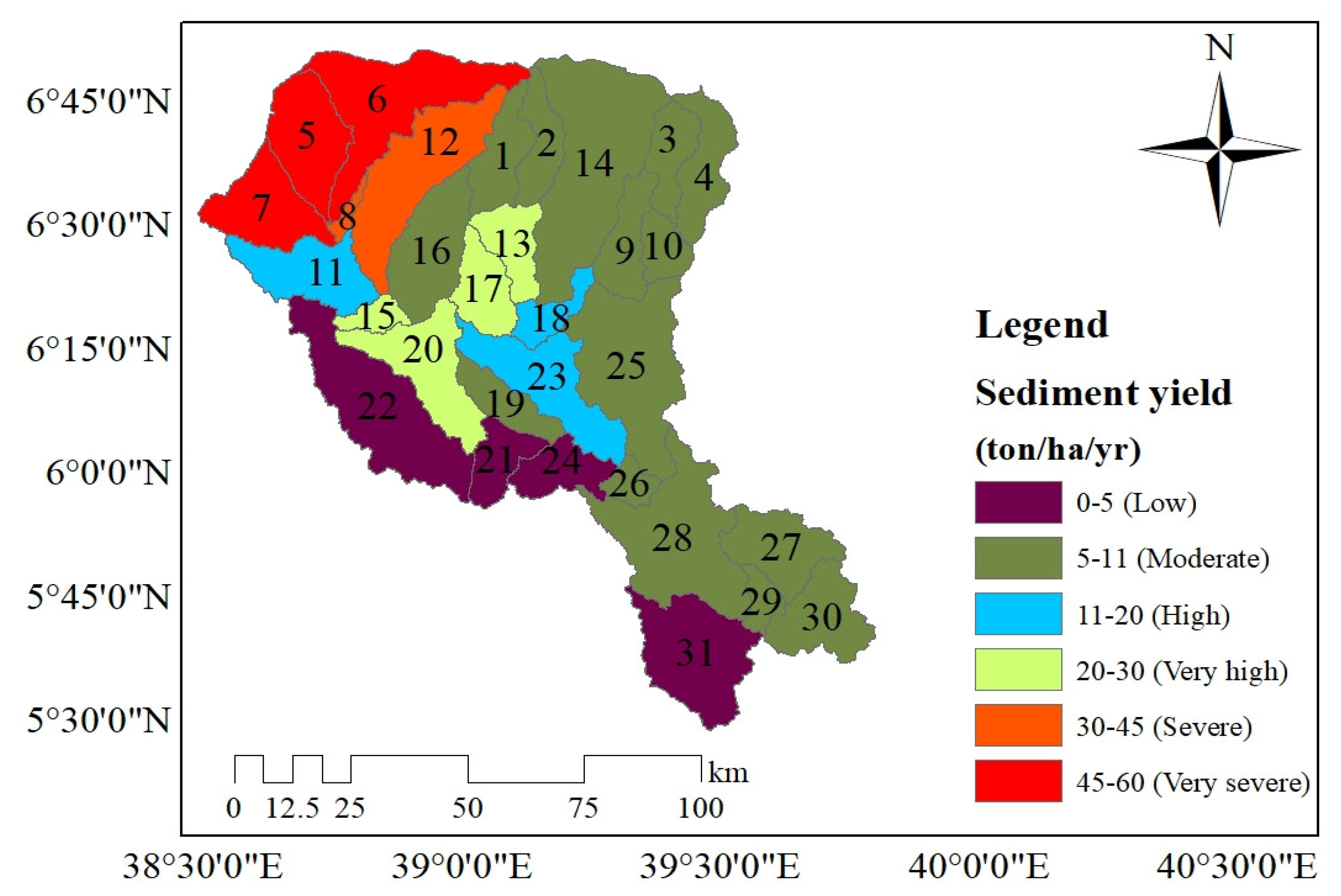
2.3.5. Scenarios for Best Management Practices (BMPs)

A SWAT model can be used to pinpoint regions with high sediment yields and adopt management strategies to reduce sedimentation problems [24]. Once the model was calibrated and validated and the results were considered acceptable, the model was ready to be parameterized to the conditions of interest. Several management activities were utilized in the SWAT model to reduce the sediment yield in the impacted subbasins. Implementing sediment management techniques in the important sediment source areas has been shown to be more effective at reducing sediment yield than randomly allocating the conservation measures to different parts of the landscape [25]. The SWAT model has also been found to be suitable for best management practices of the watershed and reported to be useful for a wide range of conditions [26]. On agricultural dominant lands, the most widely used sediment management practices are filter strips, terracing, stone/soil bund, and contour farming [27]. Hence, by comparing those widely used sediment yield reduction options, scenarios were developed and applied in the SWAT model. Then, the model was used to estimate the soil loss under different scenarios of BMPs in comparison to the existing baseline condition. The selected sediment management options were applied to sediment-prone subbasins that generated high sediment yields. These subbasins were located using the calibrated SWAT model’s spatial sediment yield mapping. The baseline values of the input parameters for the evaluation of BMPs were selected through model calibration and suggested values from previously conducted local studies [27]. Four scenarios were performed to compare the effects of sediment reduction on the critically affected subbasins in the Genale Dawa-3 dam watershed (Table 4).

Scenario 0: Baseline Scenario

This scenario was portrayed by the actual conditions found in the watershed (without soil conservation measures). Without changing any modeling parameters, the SWAT model’s calibrated values were used in this simulation. To understand the implications of various management practice scenarios on the reduction of sediment yield in the watershed, this simulation served as a starting point.

Scenario 1: Filter Strip

The filter strip was taken into consideration since planting grasses along croplands and pasture lands slows down runoff, reduces sheet and rill erosion, increases infiltration capacity and base flow, and increases the effectiveness of sediment trapping [28]. SWAT modeled the trapping effectiveness of the strip as a function of its width using Equation (8) [29]. FILTERW is an excellent model parameter for representing the impact of filter strips (width of filter strip). The SWAT management database (.mgt) was given the filter width value, FILTERW, of 1 m to model the effect of filter strips on sediment trapping. The FILTERW value was modified based on previous local research experiences in the Ethiopian watershed [27].
T r a p e f f = 0.367 × ( w i d t h f i l t e r   s t r i p ) 0.2967
where T r a p e f f is the trapping efficiency of the filter strip and w i d t h f i l t e r   s t r i p is the width of the filter strip in m.

Scenario 2: Stone/Soil Bund

The stone/soil bund practice reduces runoff and soil loss by reducing the slope length and creating retention areas [30]. The effect of stone/soil bund practice in the Genale Dawa-3 dam watershed was represented by adjusting the curve number (CN2), slope length (SLSUBBSN), and management support practice (USLE_P) parameters. The modified values of the stone/soil bund parameters were obtained from the previous local research experience in Ethiopia [31]. To test their effects, the curve number (CN2) was reduced by 3 units, slope length (SLSUBBSN) reduced by 50% and practice factor (USLE_P) set to 0.32. In the SWAT model, the HRU (.hru) input table was edited to adjust the value of the SLSUBBSN; the USLE_P and CN2 values were adjusted by editing the management (.mgt) input table.

Scenario 3: Terracing

Terracing is constructed across the slope on a contour with several regular spaces. Runoff and soil loss increase with the increase in slope length and steepness. Hence, by adjusting both erosion and runoff parameters, terracing was simulated in the SWAT model. The curve number (CN2), management support practice (USLE_P), and slope length (SLSUBBSN) were used to simulate the effect of terracing.
During simulation, the slope length (SLSUBBSN) was reduced by 50%, the curve number (CN2) was reduced by 3 units, and the practice factor (USLE_P) was set to 0.14 for land slope class of 12–16% [18]. In the SWAT model, the HRU (.hru) input table was edited to adjust the value of the SLSUBBSN; the CN2 and USLE_P values were adjusted by editing the management (.mgt) input table.

Scenario 4: Contour Farming

This practice helps to reduce surface runoff by impounding water in small depressions and through the reduction of sheet and rill erosion. Appropriate parameters used to simulate contour farming are the curve number (CN2) and management support practice (USLE_P) [30]. In this study, we tested their effects by reducing the curve number (CN2) by 3 units and adjusted the practice factor (USLE_P) with 0.5 and 0.6.

3. Results and Discussion

3.1. Streamflow Simulation

3.1.1. Model Parameter Sensitivity Analysis for Streamflow

A global sensitivity analysis was used to identify the most sensitive parameters. A total of 20 parameters were initially chosen for the sensitivity analysis, and 14 parameters had a significant impact on the streamflow simulation (based on the values of t-stat and the p-values) (Table 5). Among the selected fourteen parameters involved in monthly parameterization, seven parameters, ALPHA_BF, CN2, CH_K2, GW_DELAY, RCHRG_DP, SLSUBBSN, and SOL_AWC showed relatively high sensitivity, and seven parameters, CANMX, SOL_K, HRU_SLP, GW_REVAP, ESCO, CH_N2, and GWQMN were moderately sensitive in the streamflow simulation (Table 5). The effect of the change of the remaining six parameters (OV_N, SOL_BD, SHALLST, REVAPMN, SURLAG, and LAT_TIME) were very small or negligible.

3.1.2. Model Calibration and Validation for Streamflow

Using SWAT CUP 2019 and SUFI-2, the model was automatically calibrated (Sequential Uncertainty Fitting Version 2 program). A good agreement occurred between the observed and simulated discharge, which was confirmed using both graphical and quantitative data. Using the model performance evaluation criteria [23] shown in Table 3, the stream flow calibration and validation at the inlet of the Genale Dawa-3 dam watershed demonstrated good performance with an R2 of 0.72, NSE of 0.7, PBIAS of −2.9%, and RSR of 0.55 for the calibration and R2 of 0.71, NSE of 0.68, PBIAS of +2.3%, and RSR of 0.56 for the validation (Table 6).
The PBIAS result shows the model had a slight overestimation (negative) during the calibration and an underestimation (positive) during the validation. Hence, the statistical model performance indicators at the Genale Dawa-3 dam watershed were slightly high in comparison to those estimated by various studies conducted in different parts of Ethiopia [28,30,31,32,33]. The difference may be due to the soil, land use, and slope steepness in the study areas.
At the Genale Dawa-3 dam watershed outlet, the SUFI-2 uncertainty measure displayed a p-factor of 0.57 and r-factor of 0.78 for the calibration and a p-factor of 0.51 and r-factor of 0.72 for the validation (Table 6). This indicated that about 57% of the measured data for the calibration and 51% of the measured data for the validation were bracketed by the 95PPU with a better strength of estimation (r-factor < 1) for both cases.
The graphical representation of the predicted and observed monthly streamflow during the calibration and validation period indicated that the SWAT model prediction was adequate over the studied range of streamflow (Figure 5). In conclusion, based on streamflow modeling, all numerical model performances (Table 6) were within an acceptable range. Moreover, the SWAT creators advised that for an appropriate hydrological calibration, the value of R2 should be greater than 0.6, NSE > 0.5, and RSR < 0.7 [34]. Hence, the overall result of the calibrated and validated streamflow model result was acceptable to apply to any water-resource-related study in the basin.

3.2. Sediment Yield Simulation

3.2.1. Model Parameter Sensitivity Analysis for Sediment Yield

The sensitivity analysis of sediment yield was conducted to pinpoint the catchment’s most sensitive variables that have an impact on the model’s results. Initially, 11 factors were chosen for sensitivity analysis, but only 8 parameters had a significant impact on sediment yield based on the t-statistics and p-values (Table 7). USLE_P, USLE_K, USLE_C, LAT_SED, CH_COV2, and ADJ_PKR were the first six parameters from that group that were very sensitive and given high priority for the calibration. PRF_BSN and SPEXP were the next two parameters, and they were moderately sensitive in the sediment yield simulation (Table 7). The rest of the parameters had very low sensitivity in the sediment yield simulation (CH_EQN, CH_COV1, and SPCON). Parameters such as USLE_P, USLE_C, USLE_K, and LAT_SED were included in upland factors whereas SPCON, SPEXP, CH _COV1, ADJ_PKR, PRF_BSN, and CH_COV2 were categorized under channel factors. The upland parameters affected sediment transport at the watershed level and were mostly in line with the land use land cover changes of the watershed. The channel factors were adjusted to increase channel sediment transport capacity and lower the amount of sediment deposition.

3.2.2. Model Calibration and Validation Results for Sediment Yield

The model calibration and validation results for sediment yield were obtained at the outlet of the watershed. Based on the model performance evaluation criteria [23] shown in Table 3, the sediment yield calibration and validation at the outlet of Genale Dawa-3 dam watershed showed a good performance with an R2 of 0.68, NSE of 0.68, PBIAS of +2.4%, and RSR of 0.57 for the calibration and an R2 of 0.66, NSE of 0.66, PBIAS of +3.5%, and RSR of 0.58 for the validation (Table 8).
The PBIAS result showed the model had a slightly underestimation (positive) in both calibration and validation periods. Hence, the estimated model performance indicators at the Genale Dawa-3 dam watershed were moderate in comparison to those estimated by different studies conducted in various parts of Ethiopia [30]. The uncertainty measure of SUFI-2 showed a p-factor of 0.48 and an r-factor of 0.56 for the calibration and a p-factor of 0.36 and an r-factor of 0.53 for the validation at the outlet of the Genale Dawa-3 dam watershed (Table 8).
The graphical representation of the predicated and measured monthly sediment yield during calibration and validation periods indicated that the SWAT model prediction was adequate over the range of sediment yields (Figure 6). It can be concluded that the SWAT model was good enough to simulate the rising and falling limb during both calibration and validation periods. The deviations between observed and simulated peaks of sediment yields were comparable to those of peaks streamflow. The finding of this research was consistent with other research reports [30]. According to [30], the underestimation of peak flows by the SWAT model leads to the underestimation of sediment peaks. Furthermore, the investigations by [35] indicated that the largest error in model estimations for sediment yield was always associated with peak flow prediction errors. They reported that the second storm effects in the SWAT model may be a cause for the highest estimation errors in peak flow, which were related to inaccuracies in sediment prediction.

3.3. Sediment Yield Rate of Genale Dawa-3 Dam Watershed

The simulation of the annual sediment yield in the Genale Dawa-3 dam watershed varied from 2.71 to 53.75 ton/ha/yr with an average sediment yield of the whole watershed estimated to be 16.83 ton/ha/yr. The corresponding mean annual sediment yield contribution of each subbasin is shown in Table 9.
The estimated sediment yield in the Genale Dawa-3 dam watershed was consistent with that of other studies done in other basins in Ethiopia, including the studies by [30] in the Finchaa catchment [33], in the Awata watershed [36], in the Bilate watershed [37], in the Megech reservoir catchment [38], in the Welmel watershed, and [39] in the Toba watershed in Ethiopia.

3.4. Spatial Variability of Sediment Yield

The assessment of the spatial variability of sediment yield is useful for catchment management planning and identifying the most erodible subwatersheds. The ranges of soil erosion rates and their corresponding classes by [38] were used in this study as thresholds to identify critical erosion hot spots in the subwatersheds. The sediment source map (Figure 5) was created using the average annual sediment yield (Table 10) based on sediment yield potential, and classes were given based on their yearly average sediment yield per coverage.
The watershed’s annual sediment yield was divided into six severity categories: low (0–5 tons per acre per year), moderate (5–11 tons per hectare per year), high (11–20 tons per hectare per year), very high (20–30 tons per hectare per year), severe (30–45 tons per hectare per year), and very severe (45–60 tons per hectare per year) (Table 10).
As shown in Table 10, the subwatersheds 5, 6, 7, 8, 11, 12, 13, 15, 17, 18, 20, and 23 made up 36.97% of the research region’s total watershed area and were classified as having high, very high, severe, and very severe soil loss (Figure 7). These subwatersheds were designated as areas with high rates of erosion in the Genale Dawa-3 dam watershed because the soil losses from them exceeded the global maximum allowable soil loss rate (>11 tons/ha/yr). From a total of 31 subwatersheds, 15 subwatersheds (1, 2, 3, 4, 9, 10, 14, 16, 19, 25, 26, 27, 28, 29, and 30) were classified as having moderate soil losses and given the moderate priority class. The annual soil loss from these subwatersheds ranged from 5 to 11 tons per hectare per year (Table 10) and covered a significant portion of the watershed (47.67% from total watershed).
Land degradation, insufficient land cover, poor land management practices (lack of soil and water conservation measures), and the cultivating of undulating slopes without conservation could be the main causes for the high sediment yields in the study basin. The tolerable soil loss that can maintain the economy and maintenance of crop production range from approximately 1 to 11 ton/ha/yr [40]. However, the study area was more susceptible to soil loss since the soil loss from these sub-watersheds exceeded this acceptable range.
Because of resource limitations, it is impossible to implement soil and water conservation measures or watershed management activities in the whole watershed at one time. In this context, the subwatersheds that are at a high risk of soil erosion should be prioritized first for treatment, to achieve the sustainable development of land and water resources in the watershed. The watershed prioritization of subwatersheds involves the ranking of the subwatersheds according to the sediment yield of each subbasin and their vulnerability to the risk of soil loss severity. Hence, based on the results, subwatersheds 5, 6, 7, 8, 11, 12, 13, 15, 17, 18, 20, and 23 were identified as erosion hot spots and prioritized for watershed management intervention (Figure 6). The total area where soil erosion exceeded the maximum tolerable erosion limit of 11 tons/ha/yr was 379,485.3 ha and covered 36.97% of the total watershed area. Therefore, priorities for watershed management intervention could be focused on high, very high, severe, and very severe soil eroded subwatersheds to minimize the effects of sedimentation in the Genale Dawa-3 hydropower dam.
The produced map (Figure 7) that depicts the high erosion areas can be utilized as a tool for decision-makers to execute appropriate soil conservation measures on particular hot spots.

3.5. Best Management Practices (BMPs) Scenario Analysis

Implementing best management practices (BMP) is a key component of watershed management intervention because it helps to reduce soil erosion and sediment movement by water. Table 11 shows the outcomes of the four best management practices applications that were examined for the study area. The mean annual sediment yield reductions for the twelve critical subbasins ranged from 30.54 tons per hectare per year to 19.84 tons per hectare per year (35.02%) under the filter strips scenario, 30.54 tons per hectare per year to 14.32 tons per hectare per year (53.11%) under the contour farming scenario, 30.54 tons per hectare per year to 10.22 tons per hectare per year (66.54%) under the soil/stone bund scenario, and 30.54 tons per hectare per year to 5.84 tons per hectare per year (80.88) under the terracing scenario (Table 11). The above four scenarios showed that terracing was more effective at reducing sediment yield than other scenarios with a mean annual sediment yield reduction of up to 80.88%. On the other hand, filter strips had the least sediment yield reduction in the selected critical subbasins, and stone/soil bund had the second-best conservation practice in the watershed.
The findings of this research can serve as a reference for decision-makers to select the best technique to reduce soil erosion and sediment load, particularly on the places that have high erosion rates. On selected high erosion risk areas, the most suitable methods are terracing followed by stone/soil bund and then contouring, and lastly the application of filter strips.
The life span of a given reservoir is a function of sedimentation. The Genale Dawa-3 dam reservoir has a life storage capacity of 2310 million m3 and the average sediment yield of the watershed is estimated as 16.83 tons/ha/yr (Table 9). Since the application of filter strips on the hot spot erosion areas decreases the sediment yield by 35.02%, contour farming by 53.11%, soil/stone bund by 66.54%, and terracing by 80.88%, they may increase the lifespan of the dam in a similar manner.

4. Conclusions

The simulation of the average annual sediment yield in the Genale Dawa-3 dam watershed for the period 1990–2015 was estimated to be 16.83 tons per hectare per year with the annual sediment yield varying from 2.71 to 53.75 tons per hectare per year. The annual soil loss rates in the Genale Dawa-3 dam watershed were classified into six soil erosion severity classes, with the watershed area of (36.97%) being classified from high to very severe soil erosion risks. These areas were characterized by a steep slope and highly cultivated land in the watershed. Additionally, 63.03% of the watershed areas fell under the category of tolerable soil loss rate for maintenance of crop production, and the areas were characterized by good plantation covers in the watershed.
The study attempted to identify soil-erosion-susceptible subwatersheds for the prioritization and evaluation of best management practices in the watershed. A prioritization map was prepared to determine the areas contributing the maximum amount of sediment yield to apply the appropriate best management practices to manage the watershed. The result showed that not all subwatersheds were found to be under an equal risk of soil erosion. In this regard, prioritization enabled us to identify subwatersheds that were at a greater risk of soil erosion. The subbasins that were predicted to face a low risk of soil loss were considered as the least prioritized areas. The majority of the least prioritized areas were characterized by good plantation covers and were located in the lowlands of the watershed.
The implementation of different BMPs showed appreciable results of sediment yield reduction, with the highest reduction simulated by the terracing scenario and the lowest reduction simulated by filter strips. Thus, the findings showed that in subwatersheds that were prone to erosion, terracing was a more effective method than other soil conservation practices. In general, the study demonstrated the need for BMPs that help foster sustainable land and water resources management as well as improve upon the life span of the Genale Dawa-3 hydropower reservoir. In summary, the results can be used as a guideline for planners, decision-makers, and any other interested parties to use an appropriate technique of soil conservation practice to minimize soil erosion, especially in areas with high erosion rates.

Author Contributions

Conceptualization, A.D. and A.O.A.; methodology, software, validation, A.D. and T.D.; formal analysis, A.D. and A.O.A.; investigation, A.D.; resources, T.D.; data curation, A.D.; writing—original draft preparation, A.D. and T.D.; writing—review and editing, A.D.; visualization, A.D.; supervision, A.O.A. and T.D.; project administration, A.D.; funding acquisition, A.D. All authors have read and agreed to the published version of the manuscript.

Funding

This research was funded by Bule Hora University College of Engineering and Technology’s Postgraduate Research Project Fund.

Data Availability Statement

Data can be provided upon request.

Acknowledgments

We would like to thank the Ethiopian Ministry of Water and Energy (MoWE) and National Meteorological Agency (NMA) for providing the streamflow, sediment data, and climate data. We also thank Tesfaye Dagne for providing the necessary information on soil and water conservation practices in the study area.

Conflicts of Interest

The authors declare that they have no conflict of interest.

References

  1. Badil, N.Z.; Eslamian, S.; Sayyad, G.A.; Hosseini, S.E.; Asadilour, M.; Askari, K.O.; Singh, V.P.; Dehghan, S. Using SWAT Model to Determine Runoff, Sediment Yield in Maroon-Dam Catchment. Int. J. Res. Stud. Agric. Sci. 2017, 3, 31–41. [Google Scholar] [CrossRef]
  2. White, R. Evacuation of Sediments from Reservoirs; ICE Publishing: London, UK, 2009. [Google Scholar] [CrossRef]
  3. Haregeweyn, N.; Bekure, M.; Atsushi, T.; Mitsuru, T.; Derege, M.; Bedru, B. Reservoir Sedimentation and Its Mitigating Strategies: A Casestudy of Angereb Reservoir (NW Ethiopia). J. Soils Sediments 2011, 12, 291–305. [Google Scholar] [CrossRef]
  4. Dananto, M.; Aga, A.O.; Yohannes, P.; Shura, L. Assessing the Water-Resources Potential and Soil Erosion Hotspot Areas for Sustainable Land Management in the Gidabo Watershed, Rift Valley Lake Basin of Ethiopia. Sustainability 2022, 14, 5262. [Google Scholar] [CrossRef]
  5. Aga, A.O.; Melesse, A.M.; Chane, B. Estimating the Sediment Flux and Budget for a Data Limited Rift Valley Lake in Ethiopia. Hydrology 2019, 6, 1. [Google Scholar] [CrossRef]
  6. Aga, A.O. Modeling Sediment Yield, Transport and Deposition in The Data Scarce Region of Ethiopian Rift Valley Lake Basin. Ph.D. Thesis, Addis Ababa Institute of Technology: Addis, Ababa, Ethiopia, 2019. [Google Scholar]
  7. Hurni, H.; Solomon, B.; Berhanu, A.; Amare, D.; Ludi, E.; Portner, B.; Birru, Y.; Gete, Z. Land Degradation and Sustainable Land Management within the Highlands of Ethiopia, Global Change and Sustainable Development. 2010, pp. 187–207. Available online: https://www.researchgate.net/publication/265645925_Land_degradation_and_sustainable_land_management_in_the_Highlands_of_Ethiopia?channel=doi&linkId=545768880cf26d5090a9ba3b&showFulltext=true (accessed on 15 August 2022).
  8. Hurni, H.; Berhe, W.A.; Chadhokar, P.; Daniel, D.; Gete, Z.; Grunder, M.; Kassaye, G. Soil and Water Conservation in Ethiopia, Guidelines for Development Agents, 2nd ed.; Elsevier: Amsterdam, The Netherlands, 2016; p. 134. [Google Scholar] [CrossRef]
  9. Aliye, M.A.; Aga, A.O.; Tadesse, T.; Yohannes, P. Evaluating the Performance of HEC-HMS and SWAT Hydrological Models in Simulating the Rainfall-Runoff Process for Data Scarce Region of Ethiopian Rift Valley Lake Basin. OJMH 2020, 10, 105–122. [Google Scholar] [CrossRef]
  10. Gete, Z. Integrated Management of Watershed Experiences in Eastern and Central Africa: Lessons from Ethiopia. In Integrated Management of Watersheds for Agricultural Diversification and Sustainable Livelihoods in Eastern and Central Africa: Lessons and Experiences from Semi-Arid South Asia: Proceedings of the International Workshop; Shiferaw, B., Rao, K.P.C., Eds.; International Crops Research Institute for the Semi-Arid Tropics: Patancheruvu, India, 2006. [Google Scholar]
  11. Aga, A.O.; Melesse, A.M.; Chane, B. An Alternative Empirical Model to Estimate Watershed Sediment Yield Based on Hydrology and Geomorphology of the Basin in Data-Scarce Rift Valley Lake Regions, Ethiopia. Geosciences 2020, 10, 31. [Google Scholar] [CrossRef]
  12. Haregeweyn, N.; Poesen, J.; Nyssen, J.; De Wit, J.; Haile, H.; Govers, G.; Deckers, J. Reservoirs in Tigray: Characteristics and Sediment Deposition Problems. Land Degrad. Dev. 2006, 17, 211–230. [Google Scholar] [CrossRef]
  13. Tamene, L.; Park, S.J.; Dikau, R.; Vlek, P.L.G. Reservoir Siltation in the Semi-Arid Highlands of Northern Ethiopia: Sediment Yield–Catchment Area Relationship and a Semi-Quantitative Approach for Predicting Sediment Yield. Earth Surf. Processes Landf. 2006, 31, 1364–1383. [Google Scholar] [CrossRef]
  14. Dutta, D.; Das, R.; Mazumdar, A. Assessment of Runoff and Sediment Yield in the Tilaya Reservoir, India Using SWAT Model. Asian J. Water Environ. Pollut. 2017, 14, 9–18. [Google Scholar] [CrossRef]
  15. Adeogun, G.; Sule, F.; Salami, W.; Bakare, T.; Mohammed, A. Sustainable Sediment Management of Upper Watershed of Jebba Dam for Improved Power Generation; Technical Report No:9; National Center for Hydropower Research and Development: Ilorin, Nigeria, 2013. [Google Scholar]
  16. Uniyal, B.; Jha, K.; Verma, K.; Anebagilu, K. Identification of Critical Areas and Evaluation of Best Management Practices Using SWAT for Sustainable Watershed Management. Sci. Total Environ. 2020, 744, 140737. [Google Scholar] [CrossRef]
  17. Arabi, M.; Frankenberger, J.R.; Engel, B.A.; Arnold, J.G. Representation of Agricultural Conservation Practices with SWAT. J. Hydrol. Processes 2008, 22, 3042–3055. [Google Scholar] [CrossRef]
  18. Arnold, J.G.; Kiniry, J.R.; Srinivasan, R.; Williams, J.R.; Haney, E.B.; Neitsch, S.L. Soil Water Assessment Tool (SWAT)Theoretical Documentation Version 2012; Texas Water Resources Institute Technical Report No.439; Texas A&M University System: College Station, TX, USA, 2012; p. 650. [Google Scholar]
  19. Neitch, S.L.; Arnold, J.R.; Kiniry, J.R.; Williams, J.R. Soil and Water Assessment Tool (SWAT) Theoretical Documentation Version 2009; Texas Water Resources Institute Technical Report No.406; Texas A&M University System: College Station, TX, USA, 2011. [Google Scholar]
  20. USDA. National Engineering Handbook; Hydrology Section 4 (Chapters 4–10); USDA: Washington, DC, USA, 1972.
  21. Williams, J.R. Sediment-Yield Prediction with a Universal Equation Using Runoff Energy Factor. In Proceedings of the Sediment Yield Workshop, USDA Sedimentation Lab., Oxford, MS, USA, 28–30 November 1972. [Google Scholar]
  22. Angstrom, A. Solar and Terrestrial Radiation.Report to the International Commission for Solar Research on Actinometric Investigations of Solar and Atmospheric Radiation. Q. J. R. Meteorol. Soc. 1924, 50, 121–126. [Google Scholar] [CrossRef]
  23. Moriasi, D.N.; Arnold, J.G.; Van Liew, M.W.; Bingner, R.L.; Harmel, R.D.; Veith, T.L. Model Evaluation Guidelines for Systematic Quantification of Accuracy in Watershed Simulations. J. Am. Soc. Agric. Biol. Eng. 2007, 50, 885–900. [Google Scholar]
  24. Aga, A.O.; Chane, B.; Melesse, A.M. Soil Erosion Modelling and Risk Assessment in Data Scarce Rift Valley Lake Regions, Ethiopia. Water 2018, 10, 1684. [Google Scholar] [CrossRef]
  25. Sharpley, A.N.; Weld, J.L.; Beegle, D.B.; Kleinman, P.J.A.; Gburek, W.J.; Moore, P.A., Jr.; Mullins, G. Development of Phosphorus Indices for Nutrient Management Planning Strategies in the United States. J. Soil Water Conserv. 2003, 58, 137–152. [Google Scholar]
  26. Gull, D.S.; Dar, A.M. Modeling Runoff and Sediment Yield in Highly Gullied Regions of Kashmir Using SWAT Model: A Case Study of Lolab Watershed. J. Civ. Eng. Forum 2020, 6, 247–258. [Google Scholar] [CrossRef]
  27. Adugna, T.; Saathoff, F.; Seleshi, Y.; Gebissa, A. Evaluating the Effectiveness of Best Management Practices in Gilgel Gibe Basin Watershed—Ethiopia. J. Civ. Eng. Archit. 2013, 7, 1240–1252. [Google Scholar] [CrossRef]
  28. Gashaw, T.; Dile, Y.T.; Worqlul, A.W.; Bantider, A.; Zeleke, G.; Bewket, W.; Alamirew, T. Evaluating the Effectiveness of Best Management Practices On Soil Erosion Reduction Using the SWAT Model: For the Case of Gumara Watershed, Abbay (Upper Blue Nile) Basin. Environ. Manag. 2021, 68, 240–261. [Google Scholar] [CrossRef]
  29. Neitsch, S.L.; Arnold, J.G.; Kiniry, J.R.; Williams, J.R. Soil and Water Assessment Tool Theoretical Documentation Version 2005; USDA: Washington, DC, USA, 2005. [Google Scholar]
  30. Dibaba, W.T.; Demissie, T.A.; Miegel, K. Prioritization of Sub-Watersheds to Sediment Yield and Evaluation of Best Management Practices in Highland Ethiopia, Finchaa Catchment. Land 2021, 10, 650. [Google Scholar] [CrossRef]
  31. Lemma, H.; Adgo, E.; Poesen, J.; Nyssen, J. Identifying Erosion Hotspots in Lake Tana Basin from a Multisite Soil and Water Assessment Tool Validation: Opportunity for Land Managers. Land Degrad. Dev. 2019, 30, 1449–1467. [Google Scholar] [CrossRef] [Green Version]
  32. Negewo, T.F.; Sarma, A.K. Spatial and Temporal Variability Evaluation of Sediment Yield and Sub-Basins / Hydrologic Response Units Prioritization on Genale. J. Hydrol. 2021, 603, 127190. [Google Scholar] [CrossRef]
  33. Kefay, T.; Abdisa, T.; Chelkeba, B. Prioritization of Susceptible Watershed to Sediment Yield and Evaluation of Best Management Practice: A Case Study of Awata River, Southern Ethiopia. Appl. Environ. Soil Sci. 2022, 2022, 1460945. [Google Scholar] [CrossRef]
  34. Santhi, C.; Arnold, J.G.; Williams, J.R.; Dugas, W.A.; Srinivasan, R.; Hauck, L.M. Validation of the SWAT Model on a Larger River Basin with Point and Nonpoint Sources. J. Am. Water Resour. Assoc. 2001, 37, 1169–1188. [Google Scholar] [CrossRef]
  35. Rostamian, R.; Jaleh, A.; Afyuni, M.; Mousavi, S.F.; Heidarpour, M.; Jalalian, A.; Abbaspour, K.C. Application of a SWAT Model for Estimating Runoff and Sediment in Two Mountainous Basins in Central Iran. Hydrol. Sci. J. 2008, 53, 977–988. [Google Scholar] [CrossRef]
  36. Ayele, M.A.; Gebremariam, B. Evaluation of Spatial and Temporal Variability of Sediment Yield on Bilate Watershed, Rift Valley Lake Basin, Ethiopia. J. Water Resour. Ocean. Sci. 2020, 9, 5–14. [Google Scholar] [CrossRef]
  37. Assfaw, A.T. Calibration, Validation and Performance Evaluation of SWAT Model for Sediment Yield Modelling in Megech Reservoir Catchment, Ethiopia. J. Environ. Geogr. 2019, 12, 21–31. [Google Scholar] [CrossRef]
  38. Tessema, Y.M.; Jasińska, J.; Yadeta, L.T.; Świtoniak, M.; Puchałka, R.; Gebregeorgis, E.G. Soil Loss Estimation for Conservation Planning in the Welmel Watershed of the Genale Dawa Basin, Ethiopia. Agronomy 2020, 10, 777. [Google Scholar] [CrossRef]
  39. Dibaba, W.T.; Ebsa, D.G. Identifying Erosion Hot Spot Areas and Evaluation of Best Management Practices in the Toba Watershed, Ethiopia. Water Conserv. Manag. 2022, 6, 30–38. [Google Scholar] [CrossRef]
  40. FAO. Soil Erosion: The Greatest Challenge to Sustainable Soil Management; FAO: Rome, Italy, 2019; 100p, ISBN 9789251314265. [Google Scholar]
Figure 1. Map of the study area.
Quaternary 05 00039 g001
Figure 2. (a) Land use map; (b) soil map of the study area.
Quaternary 05 00039 g002
Figure 3. (a) The digital elevation model; (b) the delineated watershed map of the area and its subbasins.
Quaternary 05 00039 g003
Figure 4. The best fit sediment rating curve for Genale Dawa-3 dam watershed.
Quaternary 05 00039 g004
Figure 5. Monthly streamflow calibration and validation (1990–2015).
Quaternary 05 00039 g005
Figure 6. Monthly sediment yield calibration and validation (1990–2015).
Quaternary 05 00039 g006
Figure 7. Spatial variability of sediment yield for Genale Dawa-3 dam watershed.
Quaternary 05 00039 g007
Table 1. Description of spatial and temporal data used for SWAT modeling in Genale Dawa-3 dam watershed.
Data TypeDescriptionPeriod/ScaleSource
DEMUsed for watershed delineation and stream networks30 m × 30 mEthiopia Ministry of Water and Energy (MoWE)
Land use/cover (LULC)The year 2015 LULC map was generated and used to quantify the hydrological process and soil erosion in a catchment30 m × 30 mLand use/land cover map derived from Landsat-8 OLI
Soil dataInclude hydraulic conductivity, soil type, texture, and available water content. In order to match the resolution of the DEM and the land use/cover map, the vector soil map was reprocessed into a 30 m raster. 2018Water Works study, Design and Supervision Enterprises of Oromia
WeatherDaily (rainfall, max and min temperature, wind speed, relative humidity, and solar radiation of 5 stations were used to derive the hydrological balance) 1987–2019National Meteorological Agency, Ethiopia (NMA)
StreamflowDaily stream flow data of Chenemasa gauging station were collected and transposed to the GD-3 outlet for calibration and validation purposes. 1990–2015Ministry of Water and Energy, Ethiopia (MoWE)
SedimentSuspended sediment concentration data from Chenemasa station were collected and transposed to the GD-3 outlet for calibration and validation purposes.1990–2015Ethiopia Ministry of Water and Energy (MoWE)
Table 2. Meteorological stations for the Genale Dawa-3 dam watershed (1987–2019).
NoStationsLat. (°N)Long. (°E)Elev. (m)Weather Elements
RFTmaxTminRHSSWS
1Kibremengist5.8738.971680
2Negele5.4239.571544XX
3Hagerselam6.4938.522809XXX
4Yirbamuda6.238.712569XXX
5Dellomena6.4239.831313XX
Note: Lat. = latitude, Long. = longitude, RF = rainfall, Tmax = maximum temperature, Tmin = minimum temperature, RH = relative humidity, SS = sunshine, WS = wind speed, √ = data available, Elev. = elevation, and X = data not available.
Table 3. Model’s performance and allowable range for both calibration and validation phase.
RatingR2NSERSRPBIAS (%)
StreamflowSediment
Very good0.75–10.75–10–0.5 < ± 10 < ± 15
Good0.65–0.750.65–0.750.5–0.6 ± 10 ± 15 ± 15 ± 30
Satisfactory0.5–0.650.5–0.650.6–0.7 ± 15 ± 25 ± 30 ± 55
Unsatisfactory < 0.5 0.5 > 0.7 ± 25 ± 55
Table 4. Description of the selected BMPs and the parameters changes in the SWAT model.
ScenariosAdjusted Parameter Value
Parameter nameCalibrated Modified
Baseline***
Filter stripFILTERW_(.mgt)01 m
Stone/soil bundUSLE_P_(.mgt)0.560.32
CN2_(.mgt)AA-3
SLSUBBSN_(.hru)A0.5 A
TerracingUSLE_P_(.mgt)0.560.14 for slope (12–16%)
CN2_(.mgt)AA-3
SLSUBBSN_(.hru)A0.5 A
Contour farmingCN2_(.mgt)AA-3
USLE_P_(.mgt)0.560.6 for slope 1–2%
0.5 for slope 3–8%
Note: * stands for parameters and their calibrated values under existing conditions; A: calibrated values.
Table 5. List of parameters used to calibrate streamflow, fitted values, parameter ranges, and sensitivity rankings.
Parameter NameDescription of ParameterRangeFitted ValueRank
v_ALPHA_BFBaseflow alpha factor (days)0–10.9391
r_CN2Initial SCS CN(II) value ± 25 % 0.082
a_CH_K2Channel effective hydraulic conductivity (mm h−1)0–15096.453
a_GW_DELAYGroundwater delay (days) ± 10 −5.954
v_RCHRG_DPDeep aquifer percolation fraction0–10.115
v_SLSUBBSNAverage slope length10–15057.696
r_SOL_AWC(..)Available water capacity of the soil layer (mm mm−1) ± 25 % 0.237
r_CANMXMaximum canopy storage (mm)0–104.138
r_SOL_K(..)Saturated hydraulic conductivity ± 25 % 0.119
r_HRU_SLPAverage slope steepness0–10.3810
a_GW_REVAPGround water revap coefficient ± 0.036 −0.00911
v_ESCOFactor for soil evaporation compensation0–10.03512
r_CH_N2Manning’s n value for the main canal0–10.3313
v_GWQMNThreshold water depth in the shallow aquifer for flow (mm)0–50002044.6514
Table 6. The statistical properties index value for monthly streamflow calibration and validation processes and model uncertainty measurements.
VariableModel Performance Indicators Uncertainty Measures
R2NSEPBIASRSRp-Factor r-Factor
Calibration period (1990–2006)0.720.7−2.90.550.570.78
Validation period (2007–2015)0.710.68+2.30.560.510.72
Table 7. List of parameters with parameter ranges, fitted values, and sensitivity rankings used for sediment calibration.
Name of Parameters Parameters Description RangeFitted ValueRank
v_USLE_PUSLE support practice factor0–10.561
v_USLE_K(..)USLE soil erodibility factor0–0.650.062
v_USLE_C(..)Minimum value of USLE_C factor applicable to the land cover0.001–0.50.123
v_LAT_SEDSediment concentration in lateral and groundwater flow (mg/L)0–1000697.784
v_CH_COV2Channel cover factor0.5–10.885
v_ADJ_PKRPeak rate adjustment factor for sediment routing in the subbasin 0–20.746
v_PRF_BSNPeak rate adjustment factor for sediment routing in main channel0–20.927
v_SPEXPExponent re-entrainment parameter for channel sediment routing 1–1.51.498
Table 8. The statistical properties index value for sediment flow calibration and validation processes and the uncertainty measurements.
VariableModel Performance IndicatorsUncertainty Measures
R2NSEPBIASRSRp-Factor r-Factor
Calibration period (1990–2006)0.680.68+2.40.570.480.56
Validation period (2007–2015)0.660.66+3.50.580.360.53
Table 9. Mean annual sediment yield of each subbasin in Genale Dawa-3 dam watershed.
SubbasinsSediment Yield (Ton/ha/Yr)SubbasinSediment Yield (Ton/ha/Yr)SubbasinSediment Yield (Ton/ha/Yr)
18.371241.452312.77
27.971322.12242.71
39.17149.98256.70
49.801528.82266.05
551.17167.55275.15
653.751725.84287.58
750.491811.26296.11
838.33195.54309.38
98.012017.56314.32
105.39214.43
1112.87224.37
Table 10. Annual soil erosion and its severity classes of Genale Dawa-3 dam watershed.
Soil Loss Range (Ton/ha/Yr)Severity ClassesArea in haArea in PercentSubwatershedsSeverity Rank
0–5Low157,70915.3621, 22, 24, 316
5–11Moderate489,279.747.671, 2, 3, 4, 9, 10, 14, 16, 19, 25, 26, 27, 28, 29, 305
11–20High132,18412.8811, 18, 20, 234
20–30Very high50,033.74.8713, 15, 173
30–45Severe60,683.65.918, 122
45–60Very severe136,58413.315, 6, 71
Table 11. Summary of developed scenarios result for twelve critical subbasins.
Critical
Subbasins
Baseline
Scenario
Average Annual Sediment Yield (Ton/ha/Yr)
Filter StripStone/Soil BundTerracingContouring
653.7536.7016.9711.9021.34
551.1732.9117.128.8824.20
750.4932.7721.0511.1230.30
1241.4527.0717.749.6725.44
838.3324.3716.448.2024.78
1528.8218.244.912.776.80
1725.8416.366.283.319.05
1322.1214.235.643.397.71
2017.5611.183.722.384.98
1112.878.273.712.364.94
2312.778.404.893.266.93
1811.267.564.152.825.36
Average30.5419.8410.225.8414.32
% reduction35.03%66.54%80.8853.11%
Publisher’s Note: MDPI stays neutral with regard to jurisdictional claims in published maps and institutional affiliations.

