


Transient Electroosmosis on a Soft Surface

Abstract
1. Introduction
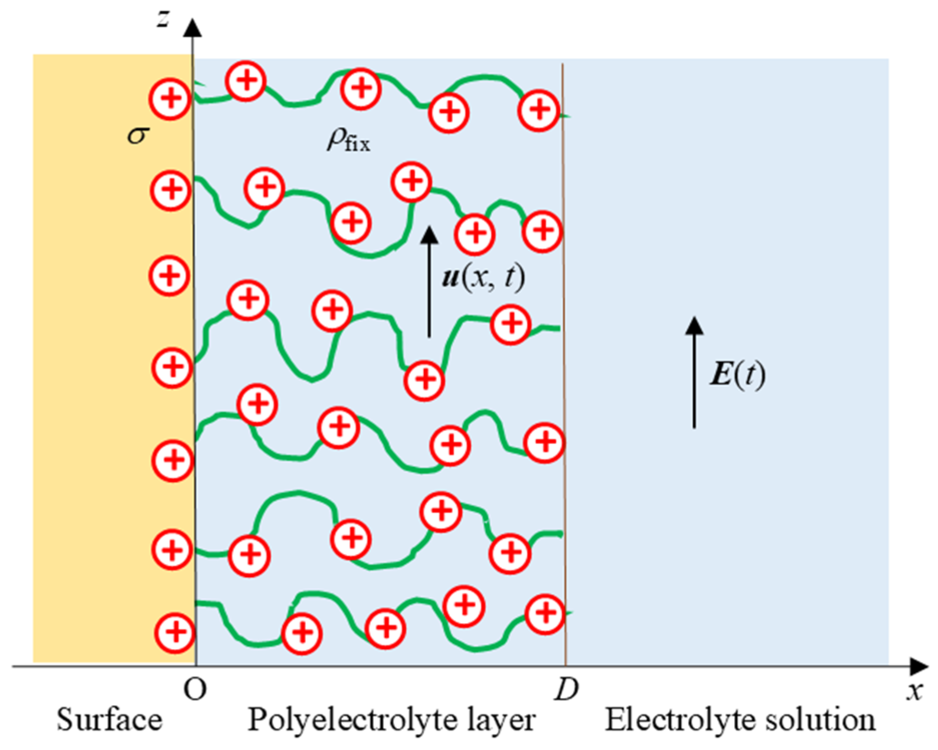
2. Theory
3. Results and Discussion
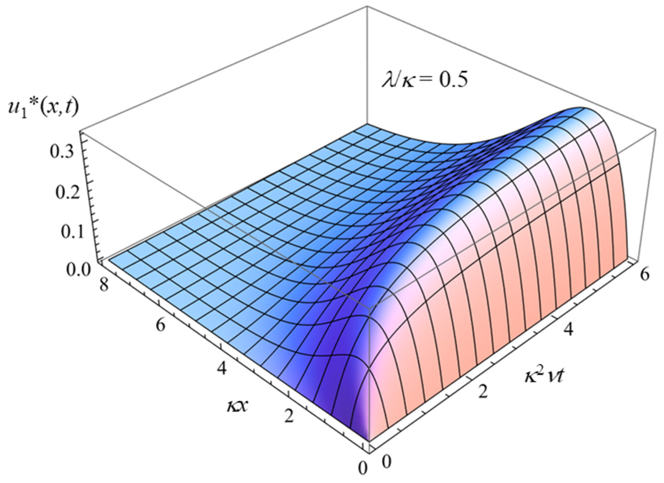
3.1. Charged Solid Surface Covered with an Uncharged Polymer Layer (σ ≠ 0 and ρfix = 0)
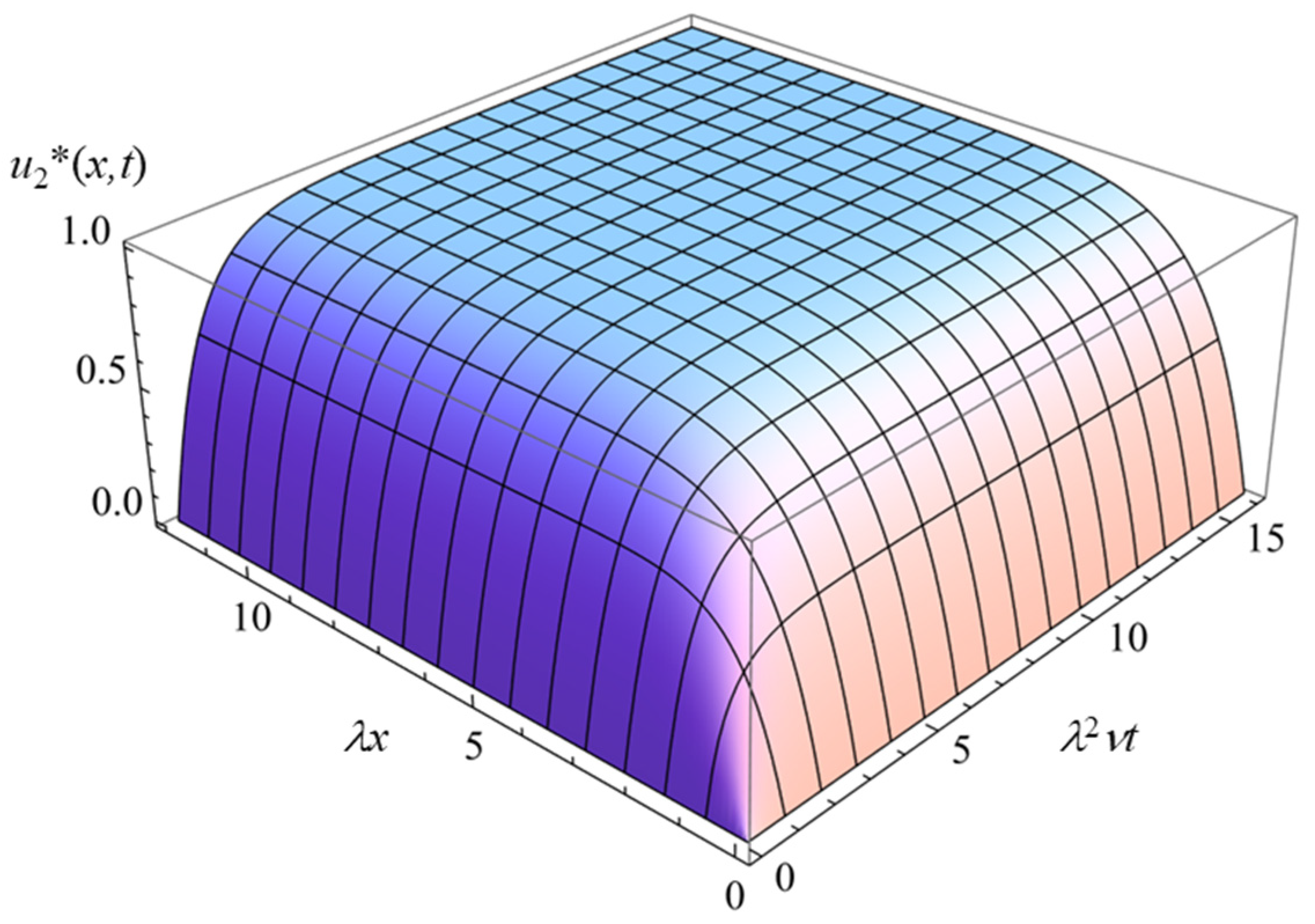
3.2. Uncharged Solid Surface Covered with a Charged Polymer (Polyelectrolyte) Layer (σ = 0 and ρfix ≠ 0)
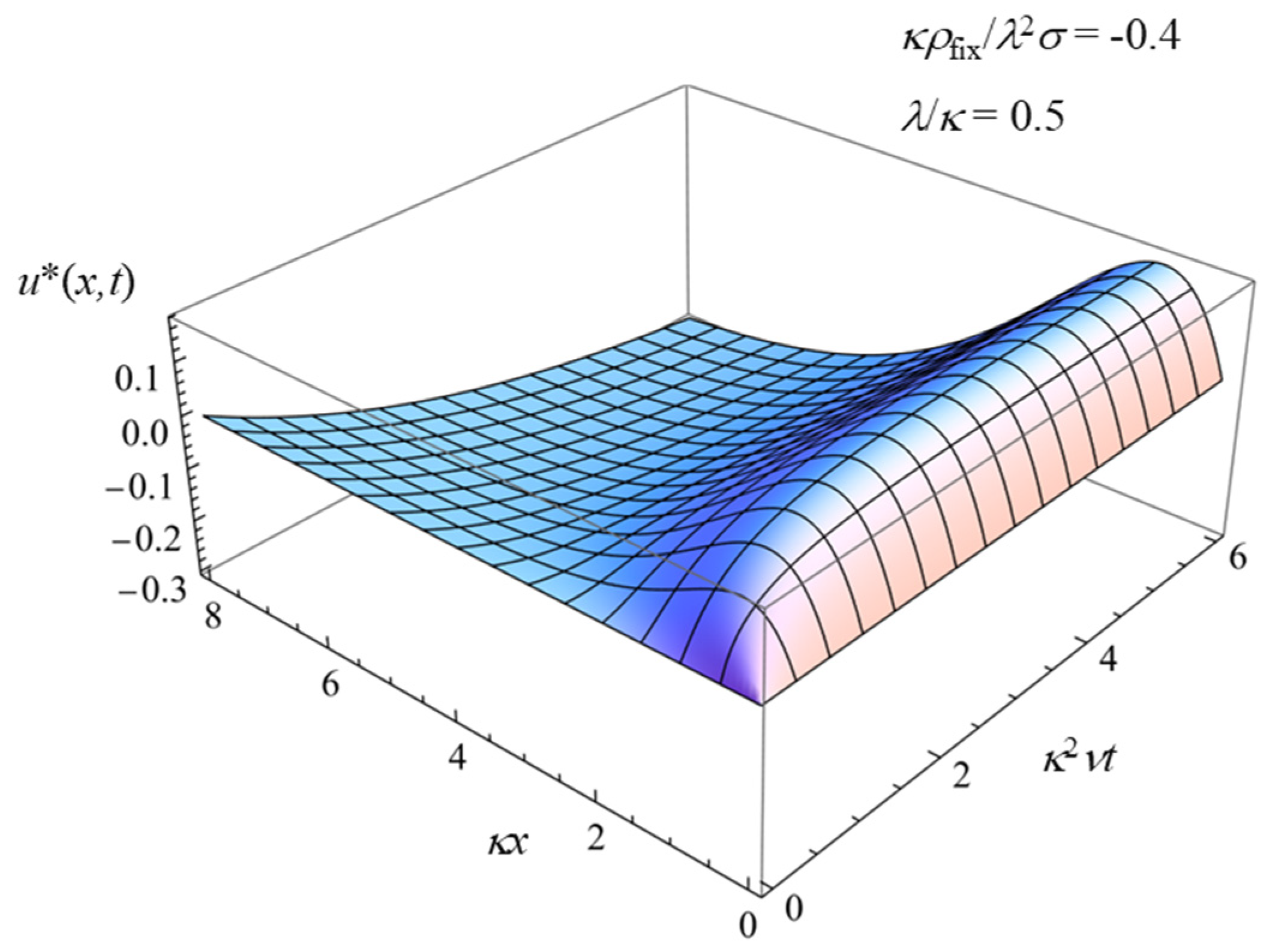
3.3. Charged Solid Surface Covered with a Charged Polymer (i.e., Polyelectrolyte) Layer (σ ≠ 0 and ρfix ≠ 0)
4. Conclusions
Funding
Data Availability Statement
Conflicts of Interest
References
- von Smoluchowski, M. Elektrische endosmose und strömungsströme. In Handbuch der Elektrizität und des Magnetismus, Band II Stationäre Ströme; Greatz, E., Ed.; Barth: Leipzig, Germany, 1921; pp. 366–428. [Google Scholar]
- Hückel, E. Die Kataphorese der Kugel. Phys. Z 1924, 25, 204–210. [Google Scholar]
- Henry, D.C. The cataphoresis of suspended particles. Part I. The equation of cataphoresis. Proc. R. Soc. Lond. Ser. A 1931, 133, 106–129. [Google Scholar]
- Booth, F. The cataphoresis of spherical, solid non-conducting particles in a symmetrical electrolyte. Proc. R. Soc. Lond. Ser. A 1950, 203, 514–533. [Google Scholar]
- Overbeek, J.T.G. Theorie der Elektrophorese. Kolloid Beih. 1943, 54, 287–364. [Google Scholar] [CrossRef]
- Wiersema, P.H.; Loeb, A.L.; Overbeek, J.T.G. Calculation of the electrophoretic mobility of a spherical colloid particle. J. Colloid Interface Sci. 1966, 22, 78–99. [Google Scholar] [CrossRef]
- O’Brien, R.W.; White, L.R. Electrophoretic mobility of a spherical colloidal particle. J. Chem. Soc. Faraday Trans. 2 1978, 74, 1607–1626. [Google Scholar] [CrossRef]
- Delgado, A.V. Interfacial Electrokinetics and Electrophoresis; Dekker: New York, NY, USA, 2001. [Google Scholar]
- Dukhin, A.S.; Goetz, P.J. Ultrasound for Characterizing Colloids. Particle Sizing, Zeta Potential, Rheology; Elsevier: Amsterdam, The Netherlands, 2001. [Google Scholar]
- Masliyah, J.H.; Bhattacharjee, S. Electrokinetic and Colloid Transport Phenomena; John Wiley & Sons: Hoboken, NJ, USA, 2006. [Google Scholar]
- Ohshima, H. Theory of Colloid and Interfacial Electric Phenomena; Elsevier: Amsterdam, The Netherlands, 2006. [Google Scholar]
- Spasic, A.; Hsu, J.-P. Finely Dispersed Particles. Micro-, Nano-, Atto-Engineering; Taylor & Francis: Milton, UK, 2005. [Google Scholar]
- Lee, E. Theory of Electrophoresis and Diffusiophoresis of Highly Charged Colloidal Particles; Elsevier: Amsterdam, The Netherlands, 2018. [Google Scholar]
- Morrison, F.A. Transient electrophoresis of a dielectric sphere. J. Colloid Interface Sci. 1969, 29, 687–691. [Google Scholar] [CrossRef]
- Morrison, F.A. Transient electrophoresis of an arbitrarily oriented cylinder. J. Colloid Interface Sci. 1971, 36, 139–145. [Google Scholar] [CrossRef]
- Ivory, C.F. Transient electroosmosis: The momentum transfer coefficient. J. Colloid Interface Sci. 1983, 96, 296–298. [Google Scholar] [CrossRef]
- Ivory, C.F. Transient electroosmosis of a dielectric sphere. J. Colloid Interface Sci. 1984, 100, 239–249. [Google Scholar] [CrossRef]
- Keh, H.J.; Tseng, H.C. Transient electrokinetic flow in fine capillaries. J. Colloid Interface Sci. 2001, 242, 450–459. [Google Scholar] [CrossRef]
- Keh, H.J.; Huang, Y.C. Transient electrophoresis of dielectric spheres. J. Colloid Interface Sci. 2005, 291, 282–291. [Google Scholar] [CrossRef]
- Huang, Y.C.; Keh, H.J. Transient electrophoresis of spherical particles at low potential and arbitrary double-layer thickness. Langmuir 2005, 21, 11659–11665. [Google Scholar] [CrossRef] [PubMed]
- Khair, A.S. Transient phoretic migration of a permselective colloidal particle. J. Colloid Interface Sci. 2012, 381, 183–188. [Google Scholar] [CrossRef] [PubMed]
- Chiang, C.C.; Keh, H.J. Startup of electrophoresis in a suspension of colloidal spheres. Electrophoresis 2015, 36, 3002–3008. [Google Scholar] [CrossRef] [PubMed]
- Chiang, C.C.; Keh, H.J. Transient electroosmosis in the transverse direction of a fibrous porous medium. Colloids Surf. A Physicochem. Engin. Asp. 2015, 481, 577–582. [Google Scholar] [CrossRef]
- Li, M.X.; Keh, H.J. Start-up electrophoresis of a cylindrical particle with arbitrary double layer thickness. J. Phys. Chem. B 2020, 124, 9967–9973. [Google Scholar] [CrossRef] [PubMed]
- Lai, Y.C.; Keh, H.J. Transient electrophoresis of a charged porous particle. Electrophoresis 2020, 41, 259–265. [Google Scholar] [CrossRef] [PubMed]
- Lai, Y.C.; Keh, H.J. Transient electrophoresis in a suspension of charged particles with arbitrary electric double layers. Electrophoresis 2021, 42, 2126–2133. [Google Scholar] [CrossRef]
- Ohshima, H. Approximate analytic expression for the time-dependent transient electrophoretic mobility of a spherical colloidal particle. Molecules 2022, 27, 5108. [Google Scholar] [CrossRef] [PubMed]
- Ohshima, H. Transient electrophoresis of a spherical soft particle. Colloid Polym. Sci. 2022, 300, 1369–1377. [Google Scholar] [CrossRef]
- Ohshima, H. Transient electrophoresis of a cylindrical colloidal particle. Fluids 2022, 7, 342. [Google Scholar] [CrossRef]
- Ohshima, H. Transient electrophoresis of a spherical colloidal particle with a slip surface. Electrophoresis 2023, 44, 1795–1801. [Google Scholar] [CrossRef]
- Saad, E.J.; Faltas, M.S. Time-dependent electrophoresis of a dielectric spherical particle embedded in Brinkman medium. Z. Angew. Math. Phys. 2018, 69, 43. [Google Scholar] [CrossRef]
- Saad, E.J. Start-up Brinkman electrophoresis of a dielectric sphere for Happel and Kuwabara models. Math. Meth. Appl. Sci. 2018, 41, 9578–9591. [Google Scholar] [CrossRef]
- Saad, E.J. Unsteady electrophoresis of a dielectric cylindrical particle suspended in porous medium. J. Mol. Liquids 2019, 289, 111050. [Google Scholar] [CrossRef]
- Sherief, H.H.; Faltas, M.S.; Ragab, K.E. Transient electrophoresis of a conducting spherical particle embedded in an electrolyte-saturated Brinkman medium. Electrophoresis 2021, 42, 1636–1647. [Google Scholar] [CrossRef]
- Ohshima, H. Fundamentals of Soft Interfaces in Colloid and Surface Chemistry; Elsevier: Amsterdam, The Netherlands, 2024. [Google Scholar]
- Brinkman, H.C. A calculation of the viscous force exerted by a flowing fluid on a dense swarm of particles. Appl. Sci. Res. 1947, 1, 27–34. [Google Scholar] [CrossRef]
- Debye, P.; Bueche, A.M. Intrinsic viscosity, diffusion, and sedimentation rate of polymers in solution. J. Chem. Phys. 1948, 16, 573–579. [Google Scholar] [CrossRef]

Disclaimer/Publisher’s Note: The statements, opinions and data contained in all publications are solely those of the individual author(s) and contributor(s) and not of MDPI and/or the editor(s). MDPI and/or the editor(s) disclaim responsibility for any injury to people or property resulting from any ideas, methods, instructions or products referred to in the content. |
© 2025 by the author. Licensee MDPI, Basel, Switzerland. This article is an open access article distributed under the terms and conditions of the Creative Commons Attribution (CC BY) license (https://creativecommons.org/licenses/by/4.0/).
Share and Cite
Ohshima, H. Transient Electroosmosis on a Soft Surface. Colloids Interfaces 2025, 9, 12. https://doi.org/10.3390/colloids9010012
Ohshima H. Transient Electroosmosis on a Soft Surface. Colloids and Interfaces. 2025; 9(1):12. https://doi.org/10.3390/colloids9010012
Chicago/Turabian StyleOhshima, Hiroyuki. 2025. "Transient Electroosmosis on a Soft Surface" Colloids and Interfaces 9, no. 1: 12. https://doi.org/10.3390/colloids9010012
APA StyleOhshima, H. (2025). Transient Electroosmosis on a Soft Surface. Colloids and Interfaces, 9(1), 12. https://doi.org/10.3390/colloids9010012