A Simple Method to Determine Critical Coagulation Concentration from Electrophoretic Mobility

Abstract

Critical coagulation concentration (CCC) is a key parameter of particle dispersions, since it provides the threshold limit of electrolyte concentrations, above which the dispersions are destabilized due to rapid particle aggregation. A computational method is proposed to predict CCC values using solely electrophoretic mobility data without the need to measure aggregation rates of the particles. The model relies on the DLVO theory; contributions from repulsive double-layer forces and attractive van der Waals forces are included. Comparison between the calculated and previously reported experimental CCC data for the same particles shows that the method performs well in the presence of mono and multivalent electrolytes provided DLVO interparticle forces are dominant. The method is validated for particles of various compositions, shapes, and sizes.

1. Introduction

Dispersions of nano or colloidal particles attract widespread contemporary interest due their extensive use in various processes in fundamental research and in more applied disciplines, in which the physico-chemical properties of the particles and the media vary in a wide range [1,2,3]. Applications include catalysis [4], energy storage [5], sensing [6], drug delivery [7] and other biomedical utilizations [8,9]; however, the stability of these dispersions is always a key issue. A typical example is the use of particles as catalysts in liquid media, where stable dispersions (i.e., homogeneously distributed primary particles) are requested during the catalytic run, while the samples can be destabilized (i.e., particle aggregation occurs) once the reaction is terminated [2,10,11]. The bigger aggregates then sediment or cream according to their density and they can be removed from the system by filtration. Moreover, aggregation of particles must be suppressed during biomedical delivery processes, since the formation of aggregates in biofluids may cause health complications such as thrombosis by blocking the veins [12,13,14]. Stable particle dispersions are also required in product manufacturing processes in the textile [15], food [16] and cosmetic [17] industry as well as in material science, where these dispersions provide processable source of particles for building up composite materials [18,19,20,21,22]. In contrast, other applications rely on destabilization of particle dispersions by induced aggregation. A typical example is secondary water treatment, in which multivalent ions and polyelectrolytes act as aggregating agents of dispersed dust particles, which sediment and hence, can be eliminated from the tanks in the aggregated form [23]. Nanoparticles can also be used to eliminate toxic contaminants from waters [24] and the removal of these particles also occurs by induced aggregation. Besides, the paper industry uses particles during production to improve certain properties of the paper and the particles undergo coaggregation with cellulose fibers in the papermaking process [25].

It is evident from the above examples that colloidal stability of particles is a key factor in most of the applications. The usual quantity to estimate colloidal stability of a particle dispersion is the critical coagulation concentration (CCC) or critical coagulation ionic strength (CCIS) indicating the necessary electrolyte concentration for the destabilization of the sample [26]. In other words, the particle collision efficiency becomes unity at the CCC, while this efficiency decreases with decreasing the concentration of the aggregating agent and becomes unmeasurable for highly stable samples, in which the particles do not form dimers after collisions. The accurate knowledge of the CCC is therefore a critical issue to estimate colloidal stability and to design stable or unstable particle dispersions. It can be determined by measuring aggregation rates of particles with a suitable technique [27]. One of the most handy methods involves light scattering either in static or dynamic mode [28]. In brief, time-resolved measurements are applied and the change in the scattered intensity or in the hydrodynamic radius can be used to calculate aggregation rate constants. These constants were also determined in turbidity measurements by following the changes of the transmittance [29] or absorbance [30] data in time-resolved experiments. A more advanced, but time-consuming approach is to measure inter-particle forces with the multi-particle colloidal probe technique based on atomic force microscopy [31]. From the primary experimental force-distance data, the rates can be calculated at different aggregating agent concentrations using appropriate theories and thus, the CCC can be determined.

The CCCs are typically strongly decreased in the presence of multivalent counterions. The correlation between valence of the counterion and CCC was observed more than 100 years ago by Schulze and Hardy [32,33]. This strong correlation is refereed to as the Schulze–Hardy rule. Later it was realized that also strongly adsorbing monovalent ions can substantially shift the CCC to lower values [34,35,36]. Therefore, the strong interaction of the counterion with the surface is the key parameter for determining the CCC. The CCC values often correlate with the magnitude of charge or electrokinetic potential of the particles, i.e., particle aggregation occurs at low magnitudes of electrokinetic potentials [37,38,39]. However, a threshold electrokinetic potential, under which the dispersion can be considered as unstable, cannot be generated for the individual systems, since aggregation processes depend on several factors including size of particles and ionic composition of the surrounding solution.

Here, we propose and implement a simple method for calculation of CCC, based on electrophoretic mobility. Electrophoretic mobility data (which are correlated with electrokinetic potentials [40]) of colloidal or nanoparticles measured at different electrolyte concentrations were used to calculate the CCC of various dispersions containing organic or inorganic charged particles of different shapes. The developed method relies on the Derjaguin, Landau, Verwey, and Overbeek (DLVO) theory, which takes into account electrostatic and van der Waals interactions. The calculated CCC values were compared to experimental ones determined independently by suitable techniques.

2. Calculating Critical Coagulation Concentration

In order to calculate the critical coagulation concentration (CCC), appropriate model has to be chosen. Here we employ DLVO theory for these calculations, since we are interested in aggregation of charged colloidal particles. In some systems non-DLVO interactions importantly shift the CCC, and in these cases the proposed approach is not applicable, as it will be seen in the results section. The DLVO theory assumes the interaction energy, V, between two charged particles to be composed of two contributions [41,42]

$$V=V_{\mathrm{vdw}}+V_{\mathrm{dl}},$$

(1)

where $V_{\mathrm{vdw}}$ and $V_{\mathrm{dl}}$ represent the van der Waals and double-layer contributions, respectively. The van der Waals interaction between two spherical particles with radius, R, can be calculated as [43,44]

$$V_{\mathrm{vdW}}=-\frac{HR}{12}·\frac{1}{h},$$

(2)

where H is the Hamaker constant and h is the surface separation distance. For the double-layer interaction Debye-Hückel superposition approximation is used

$$V_{\mathrm{dl}}=2\pi R\epsilon {\epsilon }_0{\psi }_{\mathrm{dl}}^2{e}^{-\kappa h},$$

(3)

where $\epsilon$ is the dielectric constant, ${\epsilon }_0$ is the vacuum permittivity, ${\psi }_{\mathrm{dl}}$ is the diffuse-layer potential, and $\kappa$ is the inverse Debye length. The latter parameter can be calculated as

$${\kappa }^2=8\pi {\ell }_{\mathrm{B}}{N}_{\mathrm{A}}{10}^{3}I,$$

(4)

where ${\ell }_{\mathrm{B}}=\frac{e_0^2}{4\pi \epsilon {\epsilon }_0{k}_{\mathrm{B}}T}$ is the Bjerrum length, $N_{\mathrm{A}}$ is the Avogadro constant, I is the ionic strength expressed in (mol/L), $e_0$ is the elementary charge, $k_{\mathrm{B}}$ is the Boltzmann constant, and T is the temperature. Within the Debye–Hückel approximation the charge density and potential of the surface are connected with

$$\sigma =\epsilon {\epsilon }_0\kappa {\psi }_{\mathrm{dl}}.$$

(5)

At CCC the repulsive energy barrier vanishes, which can be mathematically written as

$$V=0\mathrm{and}\frac{\mathrm{d}V}{\mathrm{d}h}=0.$$

(6)

Combining Equations (1)–(5) with conditions in Equation (6) permits to calculate the critical coagulation ionic strength (CCIS) [39]

$$\mathrm{CCIS}=\frac{1}{8\pi {\ell }_{\mathrm{B}}}·{\left(\frac{24\pi }{He\epsilon {\epsilon }_0}\right)}^{2/3}{\sigma }^{4/3},$$

(7)

where $e=2.7182\dots$ is the base of the natural logarithm. Equation (7) can be use to calculate the ionic strength, which corresponds to the CCC. In order to convert the CCIS to the CCC the relation between ionic strength and concentration has to be used

$$I=\frac{1}{2}\sum _i{c}_i{z}_i^2,$$

(8)

where $c_i$ is the concentration of all ionic species in the solution and $z_i$ is their valence. The relation between CCIS and the surface charge density given in Equation (7) has been tested on different types of particles and different electrolytes and gives relatively accurate results [34,36,39,45]. This analysis requires to first measure the CCC and then measure the surface charge density at the CCC. Here we propose a simple numerical procedure, which is able to predict the CCC from the measurements of electrophoretic mobility as a function of salt concentration. Electrophoretic mobility, $\mu$, is converted to electrokinetic potential, $\zeta$, via Smoluchowski equation [44]

$$\zeta =\frac{\mu \eta }{\epsilon {\epsilon }_0}\approx {\psi }_{\mathrm{dl}},$$

(9)

where $\eta$ is the solvent viscosity. The electrokinetic potential is usually a good approximation for the diffuse layer potential especially if the potentials are relatively low [46,47]. Note that van der Waals and double-layer interaction energies written above correspond to the case of spherical colloids. As long as the dimensions of the particles are larger than the diffuse-layer thickness at the CCC, the Derjaguin approximation is valid and one can use the corresponding effective radii in the equations [44]. For small particles of arbitrary shape however some inaccuracies steaming from the use of Derjaguin approximation can be expected.

Based on the equations written above one can construct a simple algorithm to calculate the CCC from electrophoretic mobility vs concentration data. The pseudo-code for this algorithm is given below:

convertmobilitytopotential	# use Equation (9)
convertconcentrationtoionic strength	# use Equation (8)
convertpotentialtosurface charge	# use Equation (5)
calculateCCISfromsurface charge	# use Equation (7)
find roots for$(\mathbf{CCIS}-\mathbf{ionic}\mathbf{strength})=\mathbf{0}$	# find where calculated ccis is equal
	# to experimental ionic strength
convert the resulting roots fromCCIStoCCC	# use Equation (8)

We have implemented this algorithm in python and the source code is available at https://github.com/colloidlab/ccc-calculator [48].

3. Results and Discussion

The data needed to calculate the critical coagulation concentration (CCC) is an array of electrophoretic mobility values with corresponding array of concentrations, electrolyte composition, viscosity of the solvent, and Hamaker constant for the measured system. All the analyzed data we show in this paper is taken from published work and the respective data sources are cited along the presented data sets.

Let us first explain the procedure for calculating the CCC in more detail. The available electrophoretic mobility data as a function of concentration of added salt is first interpolated by fitting an appropriate interpolating function. Typically a function describing a log-normal distribution works well in majority of the cases. An example of such an interpolation is shown in Figure 1a, where electrophoretic mobility data is shown for positively and negatively charged latex particles in NaCl solutions.

With increasing salt concentration, the electrophoretic mobility for both particles tends to zero as the particle charge is screened by addition of salt. At low salt levels the particle suspensions are stable and the stability ratios are well above 1; see Figure 1b. At increased concentrations one can observe the transition from stable to unstable suspensions and at this transition the stability ratio reaches unity. The concentration where this transition happens is refereed to as the CCC. One can also calculate the ionic strength at this concentration using Equation (8), we refer to this value as critical coagulation ionic strength (CCIS). The interpolation functions shown in Figure 1 are used to calculate the CCCs by the procedure described above. The resulting calculated CCCs for amidine and sulfate latex particles are, 225 mM and 460 mM respectively. These values are marked with arrows in Figure 1b and match perfectly with the experimentally measured stability ratios.

In Figure 1c,d results for titania nanosheets at two different pH are shown [49]. These particles are postively charged at pH 4.0 and negatively charged at pH 10. Again the calculated CCCs marked with arrows in Figure 1d match perfectly the experimental data. The examples shown in Figure 1 confirm that our method for calculating CCCs gives good results for positively and negatively charged as well as organic and inorganic particles in the presence of simple monovalent electrolytes.

Let us now look at examples, where monovalent and multivalent ions strongly adsorb to particles surfaces. In the first case, shown in the top panel of Figure 2, negatively charged sulfate latex particles are in contact with 1-hexyl-3-methylimidazolium (HMIM${}^{+}$) or 1-octyl-3-methylimidazolium (OMIM${}^{+}$) ions.

The particles are negatively charged at low concentrations and undergo charge-reversal at increased concentrations. This strong adsorption of imidazolium based ions is reflected also in stability of suspensions; see Figure 2b. The particles are stable at low concentration and aggregate fast close to charge-neutralization point after which they re-stabilize due to overcharging and finally become unstable again at high salt levels. This behavior gives rise to three CCCs. Our method can predict three CCCs for each salt and they are marked with red and green arrows, respectively. Similarly, the charge reversal is observed for amidine latex particles in the presence of Fe(CN)${}_6^{3-}$ and Fe(CN)${}_6^{4-}$ multivalent anions; see Figure 2c. Again multiple CCCs are present and can be predicted relatively accurately with the proposed method (see positions of the arrows in Figure 2d). However, the accuracy of predictions for strongly adsorbing ions is in some cases lower. For example, in the case of HMIMCl the third CCC is predicted at $\sim 400$ mM while it is observed below 100 mM. These deviations are probably related to non-DLVO interactions, which are not taken into account in our simple method, however they have been shown to be important in similar systems [50,51,52]. Albeit some inaccuracies, our proposed method for calculating CCCs is still able to quantitatively predict CCCs in most cases.

In the following we focus more on quantitative aspects of the proposed method. In Figure 3 calculated versus measured CCCs are shown for seven different types of particles at different conditions.

This analysis enables us to judge the quantitative accuracy of the proposed method. The results for different types of organic and inorganic particles as well as spherical and layered materials are shown. For each system CCCs resulting from the aggregation induced by different ions are shown. All the calculations for a specific system are done with one value for Hamaker constant. These Hamaker constants need to be adjusted because theoretical values of Hamaker constants are either not known or they can overestimate the magnitude of the van der Waals force. The Hamaker constants used for polystyrene latex particles shown in Figure 3a–c are between 2 and $3·{10}^{-21}$ J. These values are in agreement with typical values for latex particles in aqueous solutions extracted from direct force measurements [51,52,53]. Note that however, the measured values are substantially lower as compared to the theoretical value for polystyrene latex calculated from the Liftsitz theory, which is equal to $9.0·{10}^{-21}$ J [53]. These deviations between the measured and calculated Hamaker constants can be explained by the surface roughness of the particles used in the experiments [53,54,55]. Therefore, the use of theoretical values of the Hamaker constants for calculation of CCCs leads to underestimation of CCCs; see Figure 3a,b,f. This procedure of adjusting the Hamaker constants for a given material therefore enables the determination of the effective Hamaker constant for the system at hand.

In the majority of the cases the points shown in Figure 3 lay very close to the diagonal line. These results confirm that our simple method is able to quantitatively predict the CCCs for a wide variety of systems. These systems include spherical, non-spherical, and platelet particles composed of different materials in the presence of simple monovalent as well as multivalent, and complex organic ions. In Figure 3f, results for coated titania nanosheets are also shown. In the presented case, the titania nanosheets were first coated with poly(diallyldimethylammonium chloride) (PDADMAC) or poly(styrene sulfonate) (PSS) polyelectrolytes and then their stability was measured as a function of NaCl concentration at pH 4.0 and pH 10 [49]. Again one can quantitatively predict the CCCs of polyelectrolyte coated particles with the Hamaker constant of $1.7·{10}^{-20}$ J, which is also used for uncoated titania nanosheets. A more detailed observation of the results shown in Figure 3 reveals that in certain cases marked deviations between calculated and measured CCCs exist. The most prominent deviation is visible in Figure 3f for titania nanosheets coated with PDADMAC at pH 10. For this system the calculation underestimates the CCC by almost an order of magnitude. In other words, the experimental system is more stable than predicted. This result is probably a consequence of some additional steric repulsion between two platelets induced by adsorbed polyelectrolytes, which is not part of our DLVO model. Other deviations include titania particles in the presence of KSCN and KNO${}_3$ salts at pH 4.0. In these cases non-DLVO interactions are probably present due to strong specific interactions of anions with the surface. In general, for the systems below the diagonal line, non-DLVO repulsions, while for the systems above this line, non-DLVO attractions are present. Therefore, these deviations can give us a further information about the presence of the non-DLVO forces.

Finally we perform some statistical analysis on the performance of the proposed calculation method. In addition to the systems shown in Figure 3 additional data points were collected and are shown in Figure 4a and in

Table A1. Table with details of the systems analyzed in the present paper. All the calculated and measured CCCs are given.

Particle	Salt	pH	Hamaker Constant (J)	Measured CCC (M)	Calculated CCC (M)	Reference
Sulfate Latex	NaCl	4.0	$9.0·{10}^{-21}$	0.12	0.21	[56]
Sulfate Latex	KCl	4.0	$9.0·{10}^{-21}$	0.11	0.21	[56]
Sulfate Latex	CsCl	4.0	$9.0·{10}^{-21}$	0.25	0.19	[56]
Sulfate Latex	MgCl${}_2$	4.0	$9.0·{10}^{-21}$	0.031	0.048	[56]
Sulfate Latex	CaCl${}_2$	4.0	$9.0·{10}^{-21}$	0.032	0.026	[56]
Sulfate Latex	BaCl${}_2$	4.0	$9.0·{10}^{-21}$	0.024	0.037	[56]
Sulfate Latex	LaCl${}_3$	4.0	$9.0·{10}^{-21}$	0.00099	0.0016	[56]
Sulfate Latex	Co(NH${}_3$)${}_6$Cl${}_3$	4.0	$9.0·{10}^{-21}$	0.00087	0.0011	[56]
Sulfate Latex	Ru(NH${}_3$)${}_6$Cl${}_3$	4.0	$9.0·{10}^{-21}$	0.00072	0.00047	[56]
Carboxyl Latex	NaCl	4.0	$2.9·{10}^{-21}$	0.061	0.061	[56]
Carboxyl Latex	KCl	4.0	$2.9·{10}^{-21}$	0.051	0.039	[56]
Carboxyl Latex	CsCl	4.0	$2.9·{10}^{-21}$	0.050	0.051	[56]
Carboxyl Latex	MgCl${}_2$	4.0	$2.9·{10}^{-21}$	0.020	0.027	[56]
Carboxyl Latex	CaCl ${}_2$	4.0	$2.9·{10}^{-21}$	0.014	0.014	[56]
Carboxyl Latex	BaCl ${}_2$	4.0	$2.9·{10}^{-21}$	0.018	0.010	[56]
Carboxyl Latex	LaCl ${}_3$	4.0	$2.9·{10}^{-21}$	0.00088	0.0010	[56]
Carboxyl Latex	Co(NH ${}_3$)${}_6$Cl${}_3$	4.0	$2.9·{10}^{-21}$	0.0020	0.0030	[56]
Carboxyl Latex	Ru(NH ${}_3$)${}_6$Cl${}_3$	4.0	$2.9·{10}^{-21}$	0.0013	0.00097	[56]
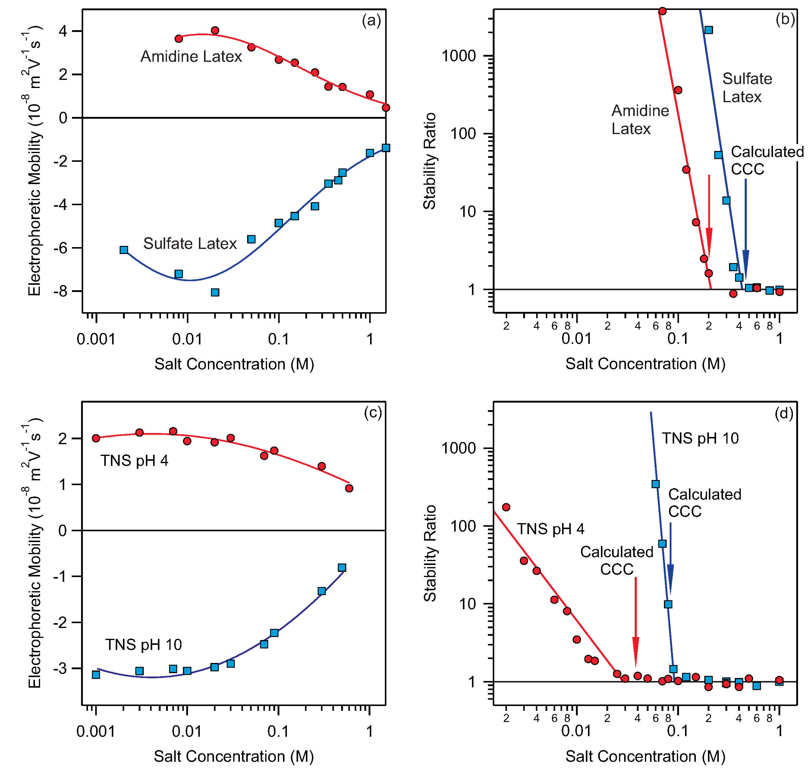
Amidine Latex	NaCl	4.0	$9.0·{10}^{-21}$	0.20	0.23	[35]
Amidine Latex	NaBr	4.0	$9.0·{10}^{-21}$	0.12	0.155	[35]
Amidine Latex	NaN(CN)${}_2$	4.0	$9.0·{10}^{-21}$	0.050	0.030	[35]
Amidine Latex	NaSCN	4.0	$9.0·{10}^{-21}$	0.052	0.044	[35]
Amidine Latex	BMIMCl	4.0	$9.0·{10}^{-21}$	0.20	0.25	[35]
Amidine Latex	BMIMBr	4.0	$9.0·{10}^{-21}$	0.15	0.194	[35]
Amidine Latex	BMIMN(CN)${}_2$	4.0	$9.0·{10}^{-21}$	0.075	0.064	[35]
Amidine Latex	BMIMSCN	4.0	$9.0·{10}^{-21}$	0.020	0.013	[35]
Amidine Latex	BMPLCl	4.0	$9.0·{10}^{-21}$	0.20	0.20	[35]
Amidine Latex	BMPLBr	4.0	$9.0·{10}^{-21}$	0.065	0.094	[35]
Amidine Latex	BMPLN(CN)${}_2$	4.0	$9.0·{10}^{-21}$	0.050	0.058	[35]
Amidine Latex	BMPLSCN	4.0	$9.0·{10}^{-21}$	0.040	0.033	[35]
Sulfate Latex	NaCl	4.0	$9.0·{10}^{-21}$	0.40	0.46	[35]
Sulfate Latex	NaBr	4.0	$9.0·{10}^{-21}$	0.40	0.46	[35]
Sulfate Latex	NaN(CN)${}_2$	4.0	$9.0·{10}^{-21}$	0.40	0.46	[35]
Sulfate Latex	NaSCN	4.0	$9.0·{10}^{-21}$	0.40	0.46	[35]
Sulfate Latex	BMIMCl	4.0	$9.0·{10}^{-21}$	0.030	0.026	[35]
Sulfate Latex	BMIMBr	4.0	$9.0·{10}^{-21}$	0.019	0.015	[35]
Sulfate Latex	BMIMN(CN)${}_2$	4.0	$9.0·{10}^{-21}$	0.036	0.038	[35]
Sulfate Latex	BMIMSCN	4.0	$9.0·{10}^{-21}$	0.093	0.062	[35]
Sulfate Latex	BMPLCl	4.0	$9.0·{10}^{-21}$	0.044	0.028	[35]
Sulfate Latex	BMPLBr	4.0	$9.0·{10}^{-21}$	0.044	0.024	[35]
Sulfate Latex	BMPLN(CN)${}_2$	4.0	$9.0·{10}^{-21}$	0.022	0.018	[35]
Sulfate Latex	BMPLSCN	4.0	$9.0·{10}^{-21}$	0.0087	0.0039	[35]
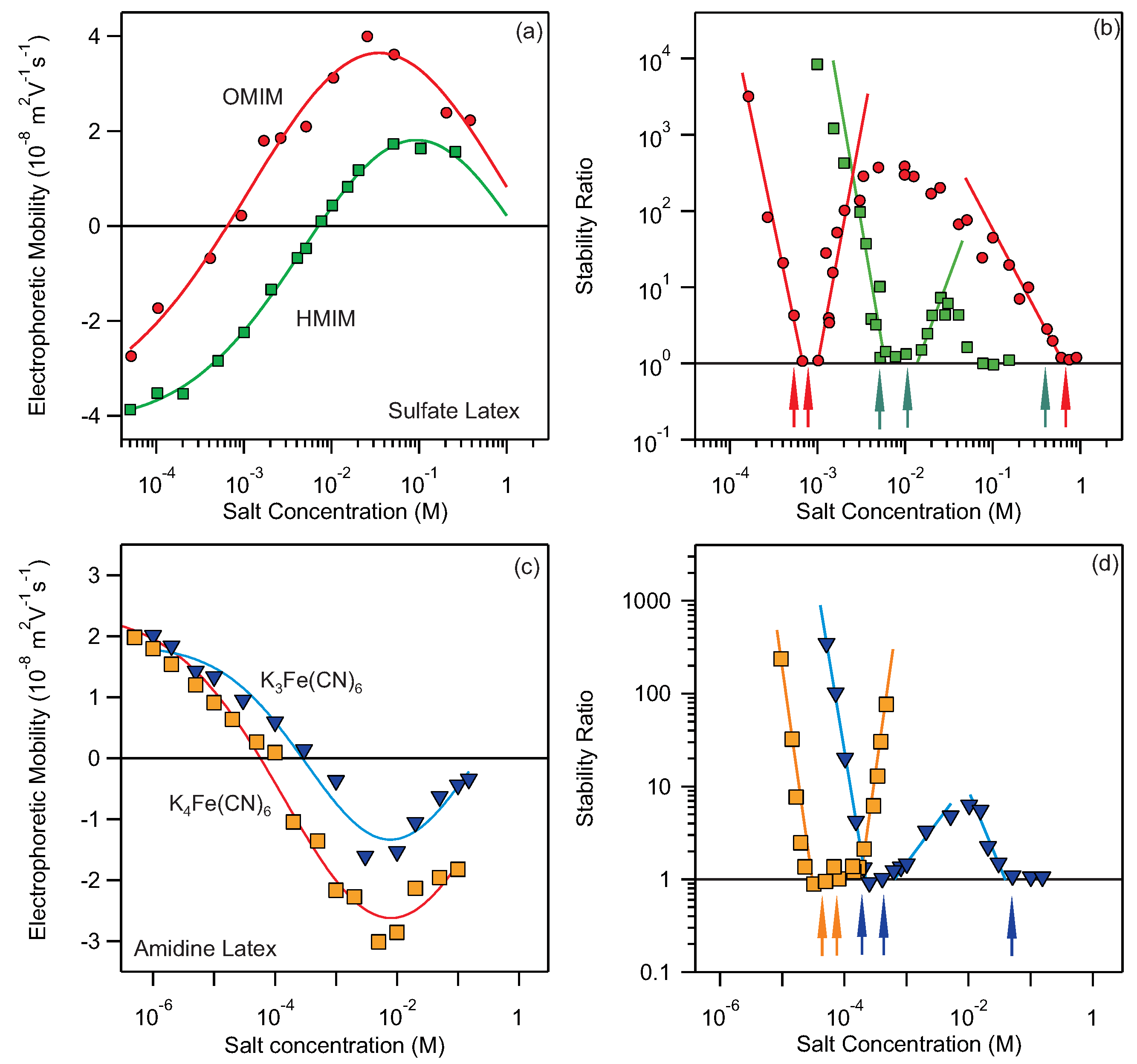
Sulfate Latex	MIMCl	4.0	$2.0·{10}^{-21}$	0.24	0.23	[35]
Sulfate Latex	EMIMCl	4.0	$2.0·{10}^{-21}$	0.151	0.125	[35]
Sulfate Latex	BMIMCl	4.0	$2.0·{10}^{-21}$	0.030	0.046	[35]
Sulfate Latex	HMIMCl	4.0	$2.0·{10}^{-21}$	0.0061	0.0051	[35]
Sulfate Latex	OMIMCl	4.0	$2.0·{10}^{-21}$	0.00071	0.00054	[35]
Amidine Latex	KCl	4.0	$3.0·{10}^{-21}$	0.25	0.18	[50]
Amidine Latex	K ${}_2$SO${}_4$	4.0	$3.0·{10}^{-21}$	0.029	0.042	[50]
Amidine Latex	K${}_3$Fe(CN)${}_6$	4.0	$3.0·{10}^{-21}$	0.00025	0.00019	[50]
Amidine Latex	K${}_4$Fe(CN)${}_6$	4.0	$3.0·{10}^{-21}$	0.000030	0.000044	[50]
Allophane	NaF	5	$3.0·{10}^{-20}$	0.00026	0.00021	[57]
Allophane	NaCl	5	$3.0·{10}^{-20}$	0.0068	0.0086	[57]
Allophane	NaBr	5	$3.0·{10}^{-20}$	0.015	0.012	[57]
Allophane	NaI	5	$3.0·{10}^{-20}$	0.017	0.0136	[57]
Allophane	NaBrO${}_3$	5	$3.0·{10}^{-20}$	0.0106	0.0117	[57]
Allophane	NaIO${}_3$	5	$3.0·{10}^{-20}$	0.0036	0.0035	[57]
Allophane	NaSCN	5	$3.0·{10}^{-20}$	0.0087	0.010	[57]
LDH	KCl	9	$1.4·{10}^{-20}$	0.054	0.060	[45]
LDH	KNO${}_3$	9	$1.4·{10}^{-20}$	0.022	0.021	[45]
LDH	KSCN	9	$1.4·{10}^{-20}$	0.013	0.0090	[45]
LDH	KHCO${}_3$	9	$1.4·{10}^{-20}$	0.0019	0.0012	[45]
TNP	KCl	10	$1.7·{10}^{-20}$	0.025	0.063	[58]
TNP	MIMCl	10	$1.7·{10}^{-20}$	0.00025	0.00042	[58]
TNP	EMIMCl	10	$1.7·{10}^{-20}$	0.016	0.018	[58]
TNP	BMIMCI	10	$1.7·{10}^{-20}$	0.028	0.027	[58]
TNP	KCl	4.0	$1.7·{10}^{-20}$	0.058	0.046	[58]
TNP	MIMCl	4.0	$1.7·{10}^{-20}$	0.056	0.037	[58]
TNP	EMIMCl	4.0	$1.7·{10}^{-20}$	0.054	0.027	[58]
TNP	BMIMCI	4.0	$1.7·{10}^{-20}$	0.040	0.042	[58]
TNS	KCl	10	$1.7·{10}^{-20}$	0.048	0.042	[58]
TNS	MIMCl	10	$1.7·{10}^{-20}$	0.00051	0.00094	[58]
TNS	EMIMCl	10	$1.7·{10}^{-20}$	0.025	0.018	[58]
TNS	BMIMCI	10	$1.7·{10}^{-20}$	0.049	0.035	[58]
TNS	KCl	4.0	$1.7·{10}^{-20}$	0.035	0.047	[58]
TNS	MIMCl	4.0	$1.7·{10}^{-20}$	0.035	0.056	[58]
TNS	EMIMCl	4.0	$1.7·{10}^{-20}$	0.037	0.061	[58]
TNS	BMIMCI	4.0	$1.7·{10}^{-20}$	0.031	0.050	[58]
TNS	NaCl	4.0	$1.7·{10}^{-20}$	0.017	0.039	[49]
TNS, PDADMAC coated	NaCl	4.0	$1.7·{10}^{-20}$	0.045	0.047	[49]
TNS, PSS coated	NaCl	4.0	$1.7·{10}^{-20}$	0.100	0.080	[49]
TNS	NaCl	10	$1.7·{10}^{-20}$	0.10	0.084	[49]
TNS, PDADMAC coated	NaCl	10	$1.7·{10}^{-20}$	0.40	0.034	[49]
TNS, PSS coated	NaCl	10	$1.7·{10}^{-20}$	0.080	0.067	[49]
TNS	KCl	4.0	$1.7·{10}^{-20}$	0.034	0.028	[36]
TNS	KNO${}_3$	4.0	$1.7·{10}^{-20}$	0.0061	0.029	[36]
TNS	KSCN	4.0	$1.7·{10}^{-20}$	0.0044	0.021	[36]
TNS	KCl	10	$1.7·{10}^{-20}$	0.039	0.045	[36]
TNS	KNO${}_3$	10	$1.7·{10}^{-20}$	0.040	0.041	[36]
TNS	KSCN	10	$1.7·{10}^{-20}$	0.052	0.064	[36]

Acronyms used in the table: LDH: layered double hydroxide, TNP: titania nanoparticles, TNS: titania nanosheets, PDADMAC: poly(diallyldimethylammonium chloride), PSS: poly(styrene sulfonate), BMPL: 1-butyl-1-methylpyrrolidinium, MIM: 3-methylimidazolium, EMIM: 1-ethyl-3-methylimidazolium, BMIM: 1-butyl-3-methylimidazolium, HMIM: 1-hexyl-3-methylimidazolium, OMIM: 1-octyl-3-methylimidazolium.

.

The data in Figure 4a show that the CCCs can be predicted relatively accurately over more than four orders of magnitude. The distribution of the relative deviation of the calculated CCCs from the measured CCCs is shown Figure 4b. Vast majority of the samples fall between the deviations of [$-40\%$, 40%]. Few samples have deviations above 100% and for these samples additional non-DLVO interactions substantially shift the CCC. Furthermore, the deviations in the positive side are more prominent. This observation can be explained by the fact that in majority of cases non-DLVO interactions, which considerably contribute to the shifting of the CCC, are attractive. Such attractive non-DLVO interactions are typically observed in systems, where ions strongly interact with the surface [50,51,52].

By taking the absolute values of the relative deviations one can construct a distribution of deviations shown in Figure 4c. The average deviation for all the sample is 38%. However, this relatively big average deviation is due to the skewed distribution. There are few samples, for which the deviation is extremely big and these points have a big influence on the average deviation. For more than 92% of the points the deviation is smaller that 0.75. For the points with the deviations larger than 0.75 the influence of the non-DLVO interactions is substantial and our proposed method is not applicable. If these points are omitted, the average deviation comes down to 25%. Bearing in mind that the error of the measurements of the CCCs is typically between 10% and 20% one can conclude that our proposed method performs surprisingly well.

Let us finally address the conventional wisdom that states that the suspensions lose their stability when the electrokinetic potential of particles reduces below 25 mV [60]. As it was already shown by some of us [39] this rule is not applicable for suspensions containing multivalent ions. Here we are further testing this simple rule by estimating the CCCs using 25 mV as a threshold of stability. The deviations between CCCs estimated from 25 mV rule and experimental CCCs are shown in Figure 5.

While the 25 mV rule works reasonably well for the CCCs between 0.1 and 1 M, the results are significantly deviating for lower concentrations. This systematic deviation is clearly evident from the fact that the points in Figure 5a follow a slope steeper than one. Furthermore, the histogram of the relative deviations presented in Figure 5b shows that the majority of points have pronounced negative deviations. The average relative deviations in this case is larger than 65%, which is much worse than our proposed method. What is even more dramatic is the systematic shift to negative deviations. The 25 mV rule is clearly unreliable for low CCCs and therefore its applicability is very limited.

4. Conclusions

In the present work, experimental electrophoretic mobility values measured in electrolyte solutions were used to calculate CCC of dispersed particles without direct determination of their aggregation rates. The developed method is based on the DLVO theory, i.e., charged particles are expected to form stable dispersions at low electrolyte concentrations due to the stabilization effect by the electrical double-layer force and the samples are destabilized above the CCC by the van der Waals attractions. For systems where the experimental Hamaker constant is not known, this parameter needs to be adjusted in order to get reliable estimations of the CCC. Therefore this method can also be used for determination of the effective Hamaker constant by measuring CCCs with different salts for the same particle system and comparing them to the calculated values.

Statistical analysis of the results and comparison to experimental CCC data determined by independent measurements revealed, that the implemented method provides CCCs, which agree very well with the experimental ones. Note that presence of non-DLVO forces may lead to certain failure of the method, as pointed out with polymer-coated particles, where steric forces provided additional stabilization of the dispersions giving rise to deviation between the calculated and experimental CCC. The method was tested for various systems including particles of different composition (polymer, metal hydroxide, and oxide), structure (sphere, sheet, and lamellar) and size (nano and colloidal particles). In addition, several types of salt solutions (ionic liquid constituents, mono and multivalent electrolytes) were used as dispersion medium. The developed method is able to determine CCC values with a deviation from the experimental values of less than 25% for majority of samples. On the other hand a simple rule based on the assumption that the CCC occurs when electrokinetic potential reaches 25 mV is much less accurate and has large systematic deviations for small CCC values, which suggests that this assumption is not physically sound.

The developed algorithm is provided as free and open source software, allowing other researchers to determine CCCs solely from electrophoretic mobility data. This tool can be of special importance in systems, in which the direct measurement of the CCC is not possible due to non-ideal sample conditions (e.g., high polydispersity, size and concentration of the particles) and also in dispersions containing electrolyte mixtures, as in many industrial and environmental processes.

References

- Bahng, J.H.; Yeom, B.; Wang, Y.; Tung, S.O.; Hoff, J.D.; Kotov, N. Anomalous Dispersions of ‘Hedgehog’ Particles. Nature 2015, 517, 596–599. [Google Scholar] [CrossRef] [PubMed]
- Scholten, J.D.; Leal, B.C.; Dupont, J. Transition Metal Nanoparticle Catalysis in Ionic Liquids. ACS Catal. 2012, 2, 184–200. [Google Scholar] [CrossRef]
- Xia, Y.; Gates, B.; Yin, Y.; Lu, Y. Monodispersed Colloidal Spheres: Old Materials with New Applications. Adv. Mater. 2000, 12, 693–713. [Google Scholar] [CrossRef]
- Herves, P.; Perez-Lorenzo, M.; Liz-Marzan, L.M.; Dzubiella, J.; Lu, Y.; Ballauff, M. Catalysis by Metallic Nanoparticles in Aqueous Solution: Model Reactions. Chem. Soc. Rev. 2012, 41, 5577–5587. [Google Scholar] [CrossRef]
- Tiwari, J.N.; Tiwari, R.N.; Kim, K.S. Zero-Dimensional, One-Dimensional, Two-Dimensional and Three-Dimensional Nanostructured Materials for Advanced Electrochemical Energy Devices. Prog. Mater. Sci. 2012, 57, 724–803. [Google Scholar] [CrossRef]
- Qin, L.; Wang, X.Y.; Liu, Y.F.; Wei, H. 2D-Metal-Organic-Framework-Nanozyme Sensor Arrays for Probing Phosphates and Their Enzymatic Hydrolysis. Anal. Chem. 2018, 90, 9983–9989. [Google Scholar] [CrossRef]
- Sokolova, V.; Epple, M. Inorganic Nanoparticles as Carriers of Nucleic Acids into Cells. Angew. Chem.-Int. Ed. 2008, 47, 1382–1395. [Google Scholar] [CrossRef]
- Masud, M.K.; Na, J.; Younus, M.; Hossain, M.S.A.; Bando, Y.; Shiddiky, M.J.A.; Yamauchi, Y. Superparamagnetic Nanoarchitectures for Disease-Specific Biomarker Detection. Chem. Soc. Rev. 2019, 48, 5717–5751. [Google Scholar] [CrossRef]
- Gu, Z.; Atherton, J.J.; Xu, Z.P. Hierarchical Layered Double Hydroxide Nanocomposites: Structure, Synthesis and Applications. Chem. Commun. 2015, 51, 3024–3036. [Google Scholar] [CrossRef]
- Ott, L.S.; Finke, R.G. Transition-Metal Nanocluster Stabilization for Catalysis: A Critical Review of Ranking Methods and Putative Stabilizers. Coord. Chem. Rev. 2007, 251, 1075–1100. [Google Scholar] [CrossRef]
- Biondi, I.; Laporte, V.; Dyson, P.J. Application of a Versatile Nanoparticle Stabilizer in Phase Transfer and Catalysis. ChemPlusChem 2012, 77, 721–726. [Google Scholar] [CrossRef]
- Abdalla, A.M.E.; Xiao, L.; Ouyang, C.X.; Yang, G. Engineered Nanoparticles: Thrombotic Events in Cancer. Nanoscale 2014, 6, 14141–14152. [Google Scholar] [CrossRef]
- Moore, T.L.; Rodriguez-Lorenzo, L.; Hirsch, V.; Balog, S.; Urban, D.; Jud, C.; Rothen-Rutishauser, B.; Lattuada, M.; Petri-Fink, A. Nanoparticle Colloidal Stability in Cell Culture Media and Impact on Cellular Interactions. Chem. Soc. Rev. 2015, 44, 6287–6305. [Google Scholar] [CrossRef] [PubMed]
- Vasti, C.; Bedoya, D.A.; Rojas, R.; Giacomelli, C.E. Effect of the Protein Corona on the Colloidal Stability and Reactivity of LDH-Based Nanocarriers. J. Mater. Chem. B 2016, 4, 2008–2016. [Google Scholar] [CrossRef] [PubMed]
- Kolman, K.; Nechyporchuk, O.; Persson, M.; Holmberg, K.; Bordes, R. Preparation of Silica/Polyelectrolyte Complexes for Textile Strengthening Applied to Painting Canvas Restoration. Colloids Surf.-Physicochem. Eng. Asp. 2017, 532, 420–427. [Google Scholar] [CrossRef]
- Dickinson, E. Food Emulsions and Foams: Stabilization by Particles. Curr. Opin. Colloid Interface Sci. 2010, 15, 40–49. [Google Scholar] [CrossRef]
- Morsella, M.; d’Alessandro, N.; Lanterna, A.E.; Scaiano, J.C. Improving the Sunscreen Properties of TiO2 through an Understanding of Its Catalytic Properties. Acs Omega 2016, 1, 464–469. [Google Scholar] [CrossRef]
- Guimaraes, T.R.; Chaparro, T.D.; D’Agosto, F.; Lansalot, M.; dos Santos, A.M.; Bourgeat-Lami, E. Synthesis of Multi-Hollow Clay-Armored Latexes by Surfactant-Free Emulsion Polymerization of Styrene Mediated by Poly(Ethylene Oxide)-Based macroRAFT/Laponite Complexes. Polym. Chem. 2014, 5, 6611–6622. [Google Scholar] [CrossRef]
- Kun, R.; Balazs, M.; Dekany, I. Photooxidation of Organic Dye Molecules on TiO2 and Zinc-Aluminum Layered Double Hydroxide Ultrathin Multilayers. Colloids Surf.-Physicochem. Eng. Asp. 2005, 265, 155–162. [Google Scholar] [CrossRef]
- Rouster, P.; Dondelinger, M.; Galleni, M.; Nysten, B.; Jonas, A.M.; Glinel, K. Layer-by-Layer Assembly of Enzyme-Loaded Halloysite Nanotubes for the Fabrication of Highly Active Coatings. Colloids Surf. B-Biointerfaces 2019, 178, 508–514. [Google Scholar] [CrossRef]
- Szabo, T.; Szekeres, M.; Dekany, I.; Jackers, C.; De Feyter, S.; Johnston, C.T.; Schoonheydt, R.A. Layer-by-Layer Construction of Ultrathin Hybrid Films with Proteins and Clay Minerals. J. Phys. Chem. C 2007, 111, 12730–12740. [Google Scholar] [CrossRef]
- Ueno, K.; Watanabe, M. From Colloidal Stability in Ionic Liquids to Advanced Soft Materials Using Unique Media. Langmuir 2011, 27, 9105–9115. [Google Scholar] [CrossRef] [PubMed]
- Bolto, B.; Gregory, J. Organic Polyelectrolytes in Water Treatment. Water Res. 2007, 41, 2301–2324. [Google Scholar] [CrossRef] [PubMed]
- Simeonidis, K.; Mourdikoudis, S.; Kaprara, E.; Mitrakas, M.; Polavarapu, L. Inorganic Engineered Nanoparticles in Drinking Water Treatment: A Critical Review. Environ. Sci.-Water Res. Technol. 2016, 2, 43–70. [Google Scholar] [CrossRef]
- Porubska, J.; Alince, B.; van de Ven, T.G.M. Homo- and Heteroflocculation of Papermaking Fines and Fillers. Colloids Surf. -Physicochem. Eng. Asp. 2002, 210, 223–230. [Google Scholar] [CrossRef]
- Elimelech, M.; Gregory, J.; Jia, X.; Williams, R.A. Particle Deposition and Aggregation: Measurement, Modeling, and Simulation; Butterworth-Heinemann Ltd.: Oxford, UK, 1995. [Google Scholar]
- Xu, S.H.; Sun, Z.W. Progress in Coagulation Rate Measurements of Colloidal Dispersions. Soft Matter 2011, 7, 11298–11308. [Google Scholar] [CrossRef]
- Trefalt, G.; Szilagyi, I.; Oncsik, T.; Sadeghpour, A.; Borkovec, M. Probing Colloidal Particle Aggregation by Light Scattering. Chimia 2013, 67, 772–776. [Google Scholar] [CrossRef]
- Kobayashi, M.; Yuki, S.; Adachi, Y. Effect of Anionic Surfactants on the Stability Ratio and Electrophoretic Mobility of Colloidal Hematite Particles. Colloids Surf. -Physicochem. Eng. Asp. 2016, 510, 190–197. [Google Scholar] [CrossRef]
- Gudarzi, M.M. Colloidal Stability of Graphene Oxide: Aggregation in Two Dimensions. Langmuir 2016, 32, 5058–5068. [Google Scholar] [CrossRef]
- Sinha, P.; Szilagyi, I.; Ruiz-Cabello, F.J.M.; Maroni, P.; Borkovec, M. Attractive Forces between Charged Colloidal Particles Induced by Multivalent Ions Revealed by Confronting Aggregation and Direct Force Measurements. J. Phys. Chem. Lett. 2013, 4, 648–652. [Google Scholar] [CrossRef]
- Hardy, W.B. A Preliminary Investigation of the Conditions Which Determine the Stability of Irreversible Hydrosols. Proc. R. Soc. Lond. 1899, 66, 110–125. [Google Scholar] [CrossRef]
- Schulze, H. Schwefelarsen in Wässriger Lösung. J. Prakt. Chem. 1882, 25, 431–452. [Google Scholar] [CrossRef]
- Oncsik, T.; Trefalt, G.; Borkovec, M.; Szilagyi, I. Specific Ion Effects on Particle Aggregation Induced by Monovalent Salts within the Hofmeister Series. Langmuir 2015, 31, 3799–3807. [Google Scholar] [CrossRef]
- Oncsik, T.; Desert, A.; Trefalt, G.; Borkovec, M.; Szilagyi, I. Charging and Aggregation of Latex Particles in Aqueous Solutions of Ionic Liquids: Towards an Extended Hofmeister Series. Phys. Chem. Chem. Phys. 2016, 18, 7511–7520. [Google Scholar] [CrossRef] [PubMed]
- Rouster, P.; Pavlovic, M.; Szilagyi, I. Destabilization of Titania Nanosheet Suspensions by Inorganic Salts: Hofmeister Series and Schulze-Hardy Rule. J. Phys. Chem. B 2017, 121, 6749–6758. [Google Scholar] [CrossRef]
- Franks, G.V. Zeta Potentials and Yield Stresses of Silica Suspensions in Concentrated Monovalent Electrolytes: Isoelectric Point Shift and Additional Attraction. J. Colloid Interface Sci. 2002, 249, 44–51. [Google Scholar] [CrossRef]
- Fernandez-Nieves, A.; Nieves, F.J.D. The Role of Zeta Potential in the Colloidal Stability of Different TiO2/Electrolyte Solution Interfaces. Colloids Surf.-Physicochem. Eng. Asp. 1999, 148, 231–243. [Google Scholar] [CrossRef]
- Trefalt, G.; Szilagyi, I.; Téllez, G.; Borkovec, M. Colloidal Stability in Asymmetric Electrolytes: Modifications of the Schulze–Hardy Rule. Langmuir 2017, 33, 1695–1704. [Google Scholar] [CrossRef]
- Delgado, A.V.; Gonzalez-Caballero, F.; Hunter, R.J.; Koopal, L.K.; Lyklema, J. Measurement and Interpretation of Electrokinetic Phenomena. J. Colloid Interface Sci. 2007, 309, 194–224. [Google Scholar] [CrossRef]
- Derjaguin, B.; Landau, L.D. Theory of the Stability of Strongly Charged Lyophobic Sols and of the Adhesion of Strongly Charged Particles in Solutions of Electrolytes. Acta Phys. Chim. 1941, 14, 633–662. [Google Scholar] [CrossRef]
- Verwey, E.J.W.; Overbeek, J.T.G. Theory of Stability of Lyophobic Colloids; Elsevier: Amsterdam, The Netherlands, 1948. [Google Scholar]
- Israelachvili, J. Intermolecular and Surface Forces, 3rd ed.; Academic Press: London, UK, 2011. [Google Scholar]
- Russel, W.B.; Saville, D.A.; Schowalter, W.R. Colloidal Dispersions; Cambridge University Press: Cambridge, UK, 1989. [Google Scholar]
- Pavlovic, M.; Huber, R.; Adok-Sipiczki, M.; Nardin, C.; Szilagyi, I. Ion Specific Effects on the Stability of Layered Double Hydroxide Colloids. Soft Matter 2016, 12, 4024–4033. [Google Scholar] [CrossRef]
- Trefalt, G.; Behrens, S.H.; Borkovec, M. Charge Regulation in the Electrical Double Layer: Ion Adsorption and Surface Interactions. Langmuir 2016, 32, 380–400. [Google Scholar] [CrossRef] [PubMed]
- Hartley, P.G.; Larson, I.; Scales, P.J. Electrokinetic and Direct Force Measurements between Silica and Mica Surfaces in Dilute Electrolyte Solutions. Langmuir 1997, 13, 2207–2214. [Google Scholar] [CrossRef]
- Trefalt, G. Ccc-Calculator. Zenodo 2020. [Google Scholar] [CrossRef]
- Sáringer, S.; Rouster, P.; Szilágyi, I. Regulation of the Stability of Titania Nanosheet Dispersions with Oppositely and Like-Charged Polyelectrolytes. Langmuir 2019, 35, 4986–4994. [Google Scholar] [CrossRef]
- Cao, T.; Sugimoto, T.; Szilagyi, I.; Trefalt, G.; Borkovec, M. Heteroaggregation of Oppositely Charged Particles in the Presence of Multivalent Ions. Phys. Chem. Chem. Phys. 2017, 19, 15160–15171. [Google Scholar] [CrossRef]
- Moazzami-Gudarzi, M.; Adam, P.; Smith, A.M.; Trefalt, G.; Szilágyi, I.; Maroni, P.; Borkovec, M. Interactions between Similar and Dissimilar Charged Interfaces in the Presence of Multivalent Anions. Phys. Chem. Chem. Phys. 2018, 20, 9436–9448. [Google Scholar] [CrossRef]
- Smith, A.M.; Maroni, P.; Borkovec, M. Attractive Non-DLVO Forces Induced by Adsorption of Monovalent Organic Ions. Phys. Chem. Chem. Phys. 2018, 20, 158–164. [Google Scholar] [CrossRef]
- Elzbieciak-Wodka, M.; Popescu, M.; Montes Ruiz-Cabello, F.J.; Trefalt, G.; Maroni, P.; Borkovec, M. Measurements of Dispersion Forces between Colloidal Latex Particles with the Atomic Force Microscope and Comparison with Lifshitz Theory. J. Chem. Phys. 2014, 140, 104906. [Google Scholar] [CrossRef]
- Valmacco, V.; Elzbieciak-Wodka, M.; Besnard, C.; Maroni, P.; Trefalt, G.; Borkovec, M. Dispersion Forces Acting between Silica Particles across Water: Influence of Nanoscale Roughness. Nanoscale Horiz. 2016, 1, 325–330. [Google Scholar] [CrossRef]
- Thormann, E. Surface Forces between Rough and Topographically Structured Interfaces. Curr. Opin. Colloid Interface Sci. 2017, 27, 18–24. [Google Scholar] [CrossRef]
- Oncsik, T.; Trefalt, G.; Csendes, Z.; Szilagyi, I.; Borkovec, M. Aggregation of Negatively Charged Colloidal Particles in the Presence of Multivalent Cations. Langmuir 2014, 30, 733–741. [Google Scholar] [CrossRef] [PubMed]
- Takeshita, C.; Masuda, K.; Kobayashi, M. The Effect of Monovalent Anion Species on the Aggregation and Charging of Allophane Clay Nanoparticles. Colloids Surf. A Physicochem. Eng. Asp. 2019, 577, 103–109. [Google Scholar] [CrossRef]
- Rouster, P.; Pavlovic, M.; Cao, T.; Katana, B.; Szilagyi, I. Stability of Titania Nanomaterials Dispersed in Aqueous Solutions of Ionic Liquids of Different Alkyl Chain Lengths. J. Phys. Chem. C 2019, 123, 12966–12974. [Google Scholar] [CrossRef]
- Bergstrom, L. Hamaker Constants of Inorganic Materials. Adv. Colloid Interface Sci. 1997, 70, 125–169. [Google Scholar] [CrossRef]
- Vallar, S.; Houivet, D.; El Fallah, J.; Kervadec, D.; Haussonne, J.M. Oxide Slurries Stability and Powders Dispersion: Optimization with Zeta Potential and Rheological Measurements. J. Eur. Ceram. Soc. 1999, 19, 1017–1021. [Google Scholar] [CrossRef]
© 2020 by the authors. Licensee MDPI, Basel, Switzerland. This article is an open access article distributed under the terms and conditions of the Creative Commons Attribution (CC BY) license (http://creativecommons.org/licenses/by/4.0/).
Share and Cite
Galli, M.; Sáringer, S.; Szilágyi, I.; Trefalt, G. A Simple Method to Determine Critical Coagulation Concentration from Electrophoretic Mobility. Colloids Interfaces 2020, 4, 20. https://doi.org/10.3390/colloids4020020
Galli M, Sáringer S, Szilágyi I, Trefalt G. A Simple Method to Determine Critical Coagulation Concentration from Electrophoretic Mobility. Colloids and Interfaces. 2020; 4(2):20. https://doi.org/10.3390/colloids4020020
Chicago/Turabian StyleGalli, Marco, Szilárd Sáringer, István Szilágyi, and Gregor Trefalt. 2020. "A Simple Method to Determine Critical Coagulation Concentration from Electrophoretic Mobility" Colloids and Interfaces 4, no. 2: 20. https://doi.org/10.3390/colloids4020020
APA StyleGalli, M., Sáringer, S., Szilágyi, I., & Trefalt, G. (2020). A Simple Method to Determine Critical Coagulation Concentration from Electrophoretic Mobility. Colloids and Interfaces, 4(2), 20. https://doi.org/10.3390/colloids4020020