Closed-Form Expressions for Contact Angle Hysteresis: Capillary Bridges between Parallel Platens

Abstract

A closed form expression capable of predicting the evolution of the shape of liquid capillary bridges and the resultant force between parallel platens is derived. Such a scenario occurs within many micro-mechanical structures and devices, for example, in micro-squeeze flow rheometers used to ascertain the rheological properties of pico- to nano-litre volumes of complex fluids, which is an important task for the analysis of biological liquids and during the combinatorial polymer synthesis of healthcare and personal products. These liquid bridges exhibit capillary forces that can perturb the desired rheological forces, and perhaps more significantly, determine the geometry of the experiment. The liquid bridge has a curved profile characterised by a contact angle at the three-phase interface, as compared to the simple cylindrical geometry assumed during the rheological analysis. During rheometry, the geometry of the bridge will change in a complex nonlinear fashion, an issue compounded by the contact angle undergoing hysteresis. Owing to the small volumes involved, ascertaining the bridge geometry visually during experiment is very difficult. Similarly, the governing equations for the bridge geometry are highly nonlinear, precluding an exact analytical solution, hence requiring a substantial numerical solution. Here, an expression for the bridge geometry and capillary forces based on the toroidal approximation has been developed that allows the solution to be determined several orders of magnitude faster using simpler techniques than numerical or experimental methods. This expression has been applied to squeeze-flow rheometry to show how the theory proposed here is consistent with the assumptions used within rheometry. The validity of the theory has been shown through comparison with the exact numerical solution of the governing equations. The numerical solution for the shape of liquid bridges between parallel platens is provided here for the first time and is based on existing work of liquid bridges between spheres.

1. Introduction

Capillary forces arising from surface tension is a frequently encountered phenomenon. This tension is due to the imbalance of forces that act on individual molecules that reside at the interface between two media. These forces may include London dispersion forces, hydrogen bonds, dipole–dipole interactions, dipole-induced dipole interactions, π-bonds, donor-acceptor bonds, and electrostatic interactions [1] and may include others. How these forces interact with the molecules and each other is complex and is not completely understood. This is because they depend very much on the substances under investigation and so many conclusions are based on empirical relationships [2].

The study of these forces is of great practical importance especially in the powder technology and related industries [3,4,5,6]. This is because moisture leads to the formation of liquid bridges between particles and so significantly affects the strength of agglomerates. Because of this, studies in this field have largely concentrated on liquid bridges between spheres [3,4,5,6,7,8,9] or between a sphere and a plane [10,11,12]. A few solutions have been proposed each using a different approximation. However, in general these solutions are not easily adaptable for modelling capillary bridges between two planes. The study of this geometry is of increasing importance as it can explain stiction in MEMS devices [13,14] and head/disk systems [15], be used for particle transfer in microfluidics channels [16], and is the geometry increasingly being used for squeeze flow rheology [17,18,19,20,21,22]. To this end, several investigators have studied capillary bridges between flat parallel surfaces [23,24,25,26,27].

It is the effect that the shape of the capillary bridge has on squeeze flow rheology that is of interest here. Generally, analysis of squeeze flow assumes that the height of the fluid layer is much smaller than its radius. This is known as the lubrication approximation [28] and allows for the assumption that the fluid flows radially. In using this approximation, it is then assumed that edge effects can be neglected. This is because dealing with the boundary conditions caused by the free surface is not a trivial matter [2,29]. However, in rheometry, the radius of the fluid is finite and so surface tension effects need to be taken into account as they influence the geometry of the fluid flow as well as imparting an additional force to the rheometer [30]. The change in the geometry of the liquid bridge caused by the movement of the platens of the rheometer manifests itself as a change in curvature of the bridge and the movement of the three-phase boundary between the liquid, the surrounding vapour phase, and the solid platen. This movement is further complicated by the effect of contact angle hysteresis which prevents the three-phase boundary from moving smoothly [26,27,31].

In order to predict the fluid flow and the forces acting on the rheometer, it is necessary to know how the shape of the liquid bridge evolves whilst it is being acted upon by a squeeze flow rheometer. To this end, this paper focuses on the derivation of a closed form expression capable of predicting the evolution of the shape of the liquid bridge during squeeze flow rheometry, including the effects of contact angle hysteresis and hence the capillary force. The validity of the theory will then be shown through comparison with an exact numerical solution.

2. Theory

In squeeze flow rheometry, when a fluid sample is placed between two parallel platens it forms a liquid bridge with a specific geometry, for instance, see Figure 1.

This is because surface tension acts to minimise the surface area of an interface. This minimisation of the surface area is described by the Young–Laplace equation [31]. This equation equates the pressure difference, $\Delta P$, across an interface between two fluids to the resulting curvature due to surface tension. For the geometry shown in Figure 1, this is most simply expressed in terms of the principal radii of curvature at the plane of symmetry of the liquid bridge, i.e., at the ‘neck’ of the bridge:

$$\Delta P=-{\gamma }_{LV}\left(\frac{1}{R_N}-\frac{1}{\rho }\right)$$

(1)

where ${\gamma }_{LV}$ is the surface tension between liquid and its vapour, and the other terms were defined in Figure 1. This pressure difference and surface tension determine the capillary force that will act on the rheometer:

$$F_{Capillary}=2\pi R_N{\gamma }_{LV}+\pi R_N^2\Delta P$$

(2)

It can be seen that this force is simply the sum of the tension acting on the surface, denoted by surface tension multiplied by the circumference of the liquid bridge, and the pressure difference acting on the cross-sectional area, see Figure 2 for a schematic.

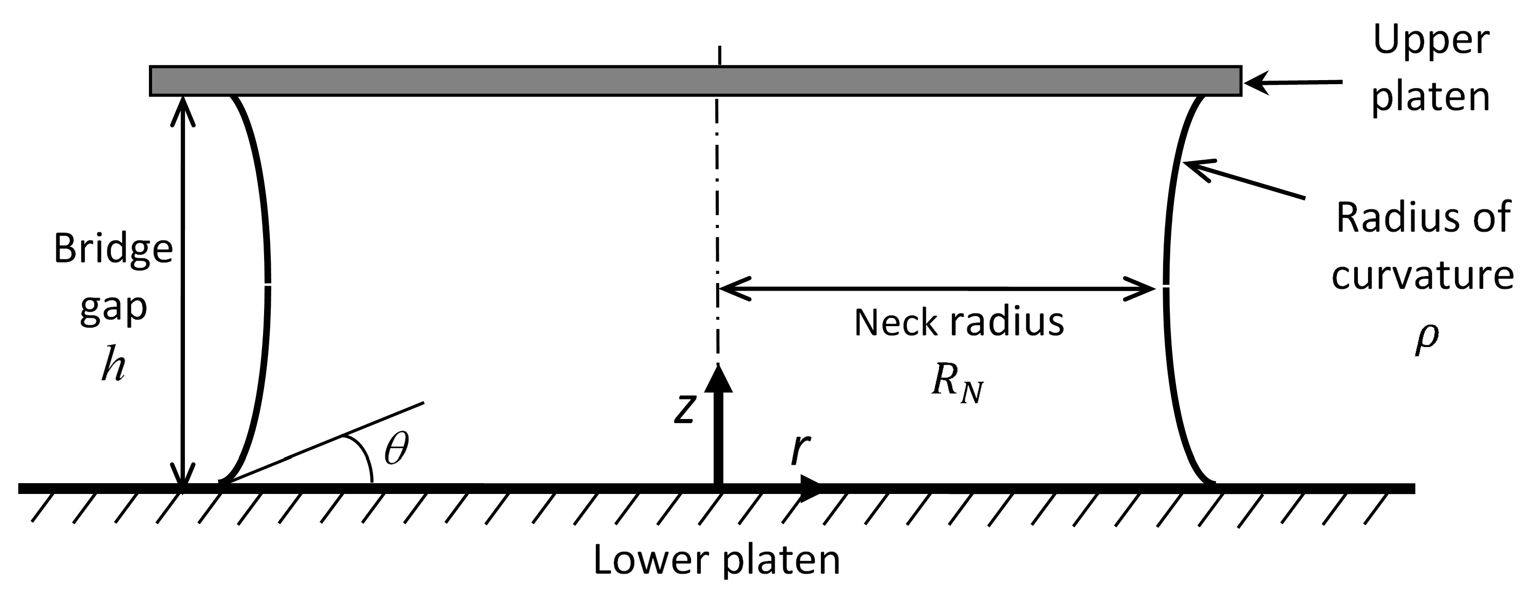
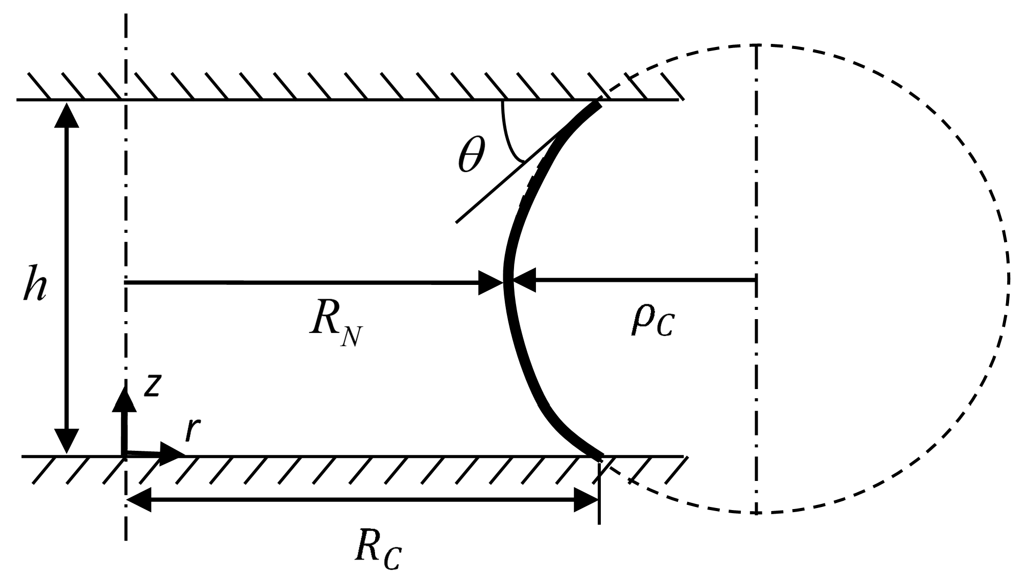
2.1. The Toroidal Approximation

The Young–Laplace equation, as given by Equation (1), cannot be solved analytically except in a few special circumstances, such as planar and cylindrical geometries [10,32]. As such, it is common practice to use numerical methods to find the solution [6]. However, a few closed form approximate solutions exist. These include the gorge approximation [6], the parabolic approximation [8], and the toroidal approximation [33]. As the parabolic approximation requires direct physical measurement of the liquid bridge (which is impractical in this case) and the gorge method leads to high inaccuracies [6], the toroidal approximation is considered the option most worth investigating. The toroidal approximation assumes the profile of the liquid bridge to be a circular arc when the Bond number is small. It has been noted that the error of the toroidal approximation can approach 10% when the bridge gap is large compared to the neck radius [34] and so a further assumption $R_N/h>1$ is sensible. It can be seen in Figure 3 that this approximation is a reasonable one. Here, as an example, the profile of a liquid bridge between two flat parallel platens with a given contact angle (45° in this case), volume ($\pi \times {10}^{-1}$ nL) and Bond number (0.002) for a range of curvatures (9500 to 52,500 m⁻¹) is shown. This profile was calculated through the numerical integration of Equation (2) using the method provided in the Appendix A. Also shown are circular arcs fitted to the ‘true’ profile representing the toroidal approximation. The circular arcs of the toroidal approximation are a good representation of the bridge profile geometry, which provides justification for the approach used here.

It is necessary to remember that the profile of the liquid bridge is not actually a circular arc. For the geometry to be valid, the mean curvature must be constant at all points on the surface of the bridge. This is not true of circular arc geometry where the curvature varies along the axis of the bridge, suggesting that a pressure difference exists within the bridge. This, of course, cannot happen or else the fluid will flow to negate the pressure difference. This means the bridge profile is not circular, but it is still a close approximation. The toroidal approximation has been used to describe the geometry of liquid bridges between spheres [35] but has not been solved completely to deal with the flat on flat geometry as is of interest here.

To use the toroidal approximation, consider the geometry for a liquid bridge between two flat platens with a gap, $h$, shown in Figure 4:

From simple geometry, the bridge profile, assumed to be a circular arc with radius ${\rho }_C$, can be expressed by the equation:

$$r\left(z\right)=R_C+\frac{h}{2}\tan \theta -\sqrt{{\rho }_C^2-{\left(\frac{h}{2}-z\right)}^2}$$

(3)

where the radius of curvature of the bridge profile is defined as:

$${\rho }_C=\frac{h}{2\cos \theta }$$

(4)

The neck radius, which is the narrowest point of the liquid bridge in the vertical axis, can therefore be defined as:

$$R_N=R_C+\frac{h}{2}\tan \theta -{\rho }_C$$

(5)

By using the disc method for calculating the volume of a revolution, the volume of the liquid bridge can be shown to be:

$$V= \underset{o}{\overset{h}{{\displaystyle \int }}}\pi {\left(R_N+{\rho }_C-\sqrt{{\rho }_C^2-{\left(\frac{h}{2}-z\right)}^2}\right)}^{2}dz$$

(6)

We can solve Equation (6), and so the neck and contact radii for a given gap, contact angle, and volume for the bridge can be shown to be:

$$R_N=\frac{1}{2}\sqrt{\frac{hA}{{\cos }^2\theta }\left(\frac{hA}{4{\cos }^2\theta }+\frac{h}{2}\tan \theta \right)+\frac{4V}{\pi h}+\frac{h^2}{12}-3{\rho }_C^2}-\left({\rho }_C-\frac{h}{4}\tan \theta -\frac{{\rho }_C^{2}A}{h}\right)$$

(7)

$$R_C=\frac{1}{2}\sqrt{\frac{hA}{{\cos }^2\theta }\left(\frac{hA}{4{\cos }^2\theta }+\frac{h}{2}\tan \theta \right)+\frac{4V}{\pi h}+\frac{h^2}{12}-3{\rho }_C^2}-\left(\frac{h}{4}\tan \theta -\frac{{\rho }_C^{2}A}{h}\right)$$

(8)

where: $A={\sin }^{-1}\left(h/2{\rho }_C\right)$.

This means we can calculate the capillary force as a function of gap for a given volume and contact angle using the definition given by Equation (9):

$$F_{CT}=2\pi R_N{\gamma }_{LV}-\pi R_N^2{\gamma }_{LV}\left(\frac{1}{R_N}-\frac{1}{{\rho }_C}\right)$$

(9)

where the neck radius and the radius of curvature are those approximately given by Equations (7) and (4).

2.2. Contact Angle Hysteresis

The above discussion is only valid when the contact angle remains constant. When the contact line is in motion, such as when the liquid in the bulk phase is flowing, as in during squeeze flow rheology, different mechanics apply. Many aspects of this dynamic wetting are poorly understood, and the subject is of great scientific interest [36]. What is known is that when the contact line moves due to flow within the bulk of the liquid, hysteresis is observed in the contact angle. As the contact line moves towards the vapour, the contact angle will become larger than the equilibrium angle; this is known as the advancing contact angle. Similarly, when the contact line contracts, the contact angle is smaller than the equilibrium value, and this is known as the receding contact angle.

It has been found that the contact line does not move smoothly, but instead pins and slips [27,37]. This is because there is a transition period as the contact angle varies between its advancing and receding state. In the context of the rheometer, this contact line will undergo four stages of motion:

1) 

When the platen moves downwards and the gap decreases, initially, the contact line remains stationary until the contact angle equals the advancing contact angle (see Figure 5a). This is known as pinning.

2) 

If the gap decreases further, the contact angle remains at the advancing angle and the contact line expands (see Figure 5b). This is known as slipping.

3) 

When the gap increases, the contact angle first decreases while the contact line remains constant (pins—see Figure 5c).

4) 

When the contact angle reaches the receding angle, provided the gap is still increasing, it will remain at that angle while the contact line declines (slips—see Figure 5d). And so on.

When the contact line slips, the contact angle remains constant and so the discussion above is valid. However, during the pining regime, the contact angle varies and so Equation (6) would need to be solved for $\theta$ as a function of the gap, $h$. This is not trivial, and an analytical solution cannot be derived. To find a solution, a numerically derived expression needs to be found. It is easy to see that the variation of the contact angle as a function of the gap will depend on the volume of the bridge and the contact line radius. Therefore, in order to obtain a single expression that will cover all situations, the equations will be non-dimensionalised by dividing all lengths and radii by the cube root of the bridge volume:

$$h^{*}=\frac{h}{\sqrt[3]{V}}, R_C^{*}=\frac{R_C}{\sqrt[3]{V}}, R_N^{*}=\frac{R_N}{\sqrt[3]{V}}$$

(10)

It is also necessary to normalise the gap between the theoretical extreme gaps for a liquid bridge with constant contact line radius and volume. These extremes correspond to the situation where the contact angle is at a maximum (180°) or a minimum (0°). These cases relate respectively to the (i) minimum gap, where any further decrease would cause the contact line to slip, and (ii) the maximum gap, where any further increase would cause the contact line to slip, as illustrated in Figure 6. A real liquid will generally oscillate between limits in-between the theoretical limits.

These extreme gaps can be found by solving Equation (6) for the gap and setting the contact angle to its relevant value. The extreme gaps in their non-dimensional form can be given as:

$$h_{min}^{*}=\frac{B}{2\pi }-\left(4-\frac{{\pi }^2}{2}\right)\frac{\pi R_C^{*2}}{B}-\frac{\pi R_C^{*}}{2}$$

(11)

where: $B=\sqrt[3]{\left(12-{\pi }^2\right){\pi }^4{R}_C^{*3}+24{\pi }^2+4{\pi }^2\sqrt{\left(32-3{\pi }^2\right){\pi }^2{R}_C^{*6}+\left(36-3{\pi }^2\right){\pi }^2{R}_C^{*3}+36}}$

and:

$$h_{max}^{*}=\left(4-\frac{{\pi }^2}{2}\right)\frac{\pi R_C^{*2}}{C}-\frac{C}{2\pi }+\frac{\pi R_C^{*}}{2}$$

(12)

where: $C=\sqrt[3]{\left(12-{\pi }^2\right){\pi }^4{R}_C^{*3}-24{\pi }^2+4{\pi }^2\sqrt{\left(32-3{\pi }^2\right){\pi }^2{R}_C^{*6}+\left(3{\pi }^2-36\right){\pi }^2{R}_C^{*3}+36}}$

The normalised dimensionless gap between the platens, $N{h}^{*}$, is thus defined as:

$$N{h}^{*}=\frac{h^{*}-h_{min}^{*}}{h_{max}^{*}-h_{min}^{*}}$$

(13)

There is also another case of special interest, which corresponds to a contact angle of 90°. When this is the case, the bridge assumes the shape of a cylinder, and is the point where the profile changes from being concave to convex and visa-versa. It is useful to note that this case represents a singularity in the solution of Equation (6), as it means that Equation (4) equals infinity (i.e., the bridge profile is straight).

There are multiple solutions to Equation (6) for a given contact line radius, but the solution which coincides with the smallest gap corresponds to that of the most stable bridge, where the effects of drainage is minimal [38]. However, when the dimensionless contact line radius, $R_C^{*}$, is less than 1, the only solutions that exist correspond to potentially unstable bridges with gaps between the platens much larger than for bridges with larger contact line radii. Due to the intractability of the solution of Equation (6), the contact angle as a function of the normalised dimensionless gap was found numerically by using a bisection method. The result can be seen in Figure 7:

The curves in Figure 7 have the shape of a generalised logistic curve, which has the form of Equation (14) (in units of degrees).

$$\theta \left(N{h}^{*}\right)=A_L+\frac{dA}{{\left(1+T{e}^{-GR\left(N{h}^{*}-M\right)}\right)}^{1/T}}$$

(14)

where $A_L$ is the lower asymptote, $dA$ is the distance between the asymptotes, $T$ affects near which asymptote maximum growth occurs, $GR$ is the growth rate and $M$ is the point of maximum growth. These variables were all found to be as functions of $R_C^{*}$. $GR$ is given in terms of a polynomial, and $A_L$, $dA$, $M,$ and $T$ can be given by Gompertz curves, the coefficients of which were found, using a standard curve fitting algorithm, to be:

$$A_L\left(R_C^{*}\right)=20568.63e^{-0.135e^{-5.496R_{C }^{*}}}-20372.76$$

$$dA\left(R_C^{*}\right)=-275719.67e^{-0.00375e^{-3.789R_{C }^{*}}}+275509.90$$

$$T\left(R_C^{*}\right)=18893.64e^{-0.000638e^{-2.3R_{C }^{*}}}-18892.64$$

(15)

$$GR\left(R_C^{*}\right)=\begin{array}{c}{200.556R_C^{*4}-967.955R_C^{*3}+1756.268R_C^{*2}-1419.955R_C^{*}+436.173|}_{R_C^{*} < 1.3}\\ {0.0359R_C^{*4}-0.296R_C^{*3}+0.537R_C^{*2}+0.248R_C^{*}+3.775|}_{R_{C }^{*}> 1.3}\end{array}$$

$$M\left(R_C^{*}\right)=4316.216e^{-0.000803e^{-2.415R_{C }^{*}}}-4315.728$$

The quality of the fit of the coefficients can be seen in Figure 8, where the coefficients of determination for each of the fits is 0.9987 or better.

The results of substituting Equation (15) into Equation (14) are shown in Figure 9:

Above $R_C^{*}=1$, the results of Equation (14) can be seen to be in good agreement with the numerically obtained results, with coefficients of determination of 0.98 or greater. This means that they can be used as working equations when dealing with the effects of contact angle hysteresis. Because Equation (15) converge to a single value as $R_C^{*}$ increases beyond 2.8, Equation (14) can be simplified to:

$$\theta \left(N{h}^{*}\right)={200.98+\frac{-210.55}{{\left(1+1.442e^{-5.771\left(N{h}^{*}-0.508\right)}\right)}^{0.693}}|}_{R_{C }^{*}> 2.8}$$

(16)

The geometry of a liquid bridge undergoing a change in height can now be calculated for the two circumstances, namely when the contact line slips and when it pins. The procedure for any subsequent calculations would be as follows:

• State initial conditions
  • We need to know four things: gap, initial contact angle, contact line radius, and volume.
  • Gap is a design/experimental parameter and is known, equilibrium (and dynamic for later) contact angle is a fluid property and can be found easily beforehand.
  • The volume or the contact line radius needs to be measured. The other can be calculated using Equations (6) or (8), respectively. However, they only need to be measured once. The values can then be used throughout the calculation.
• Change the gap
  • It is assumed that subsequent motion will be continuous and no relaxation towards equilibrium conditions is observed.
  • The change in geometry depends on the direction the upper platen is moved.
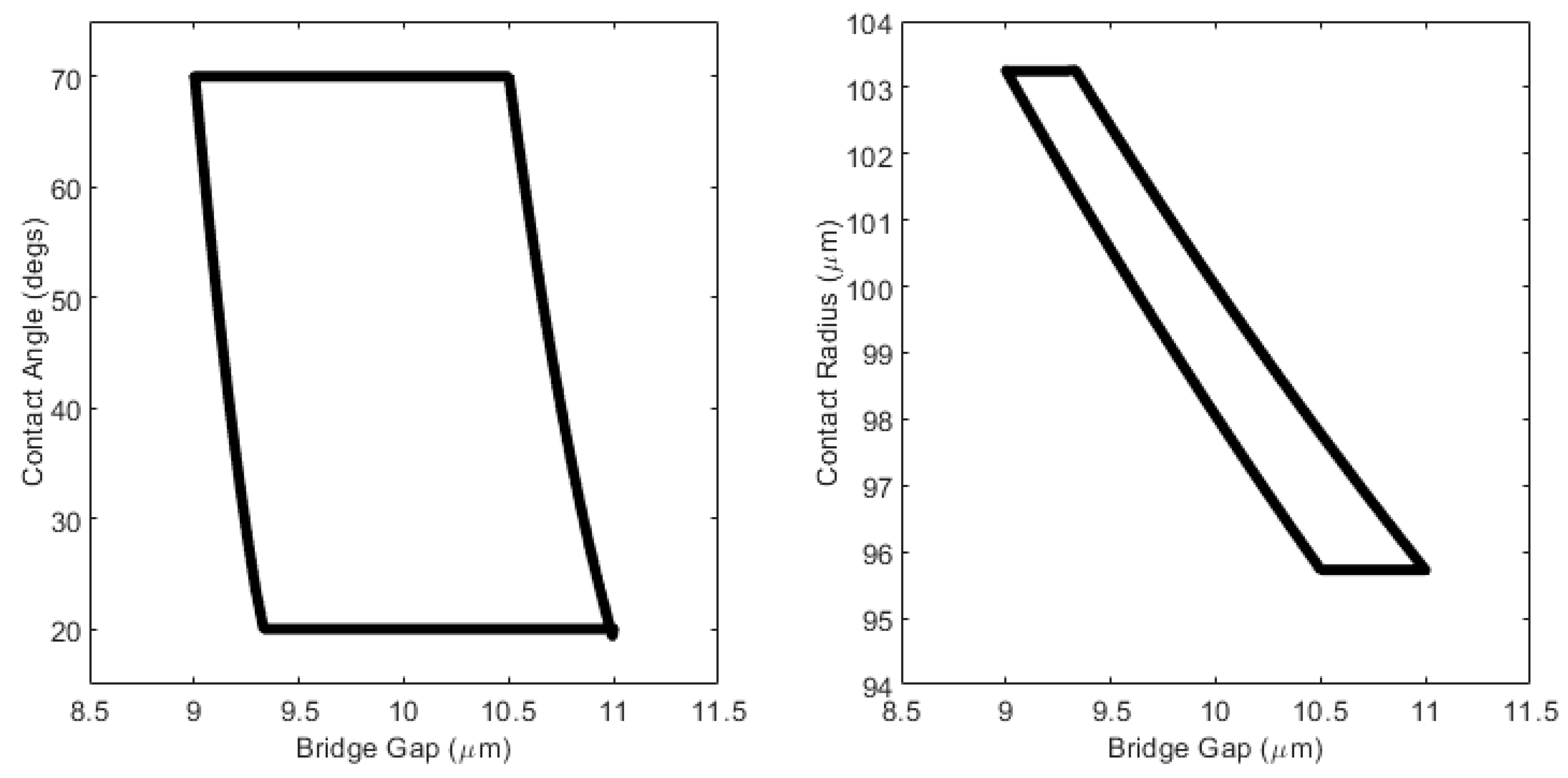
  • If it is moving upwards, initially, the receding contact angle will be lower than the equilibrium contact angle. Here, the contact line radius (given) will stay constant until the instantaneous contact angle (given by Equation (16)) equals the receding contact angle. If the motion continues to increase, the contact angle stays constant and the contact line radius changes according to Equation (8).
• Change the direction
  • At this point, the contact angle equals the receding contact angle and the contact line radius is known. Decreasing the gap, the contact line radius will remain constant and the contact angle will increase, as in Equation (16), until it reaches the advancing contact angle. Decreasing the gap further will mean the contact angle stays at the advancing angle and the contact line radius changes.

Using this procedure, the capillary forces can be found, as demonstrated in Figure 10 for two scenarios covering a wide range of contact angle hysteresis.

The maximum relative error between the force as calculated using the toroidal approximation and that calculated numerically from the exact expression using the algorithm given in the Appendix A, is 0.21% for the data shown in Figure 10 (left) and 1.3% in Figure 10 (right).

Significantly, the data in Figure 10 (left) (that is, the 120 data points used to describe one cycle here) took c.a. 880 s to generate using MATLAB R2018a on a HP Omen Laptop with Intel^® Core™ i7-9750H CPU @ 2.60GHz, with 6 Cores, 12 Logical Processors and 16 GB of RAM. The equivalent data generated on the same system using Equation (14) took just c.a. 0.12 s. This demonstrates the significant speed-up the use of these closed-form expressions can give the user as compared to having to solve the exact equations numerically.

It can be clearly seen that the form of these curves is very similar to those measured experimentally by De Souza et al. [26] and by Shi et al. [27]. Direct comparison is not possible between these studies and the theory proposed here as those studies used asymmetric bridges with large bond numbers and large extensions/velocities in which viscous forces and bridge collapse is significant and not of interest here. For the case shown in Figure 10, the contact line radius and contact angle, as calculated using the toroidal approximation, vary as a function of gap and are as shown in Figure 11 and Figure 12:

This relationship may be better appreciated as a function of time:

Figure 12. Variation of contact angle (left) and contact line radius (right) as a function of time for the scenario demonstrated in Figure 10 (left). In this case, a frequency of 10 Hz is arbitrarily assumed.

Figure 12. Variation of contact angle (left) and contact line radius (right) as a function of time for the scenario demonstrated in Figure 10 (left). In this case, a frequency of 10 Hz is arbitrarily assumed.

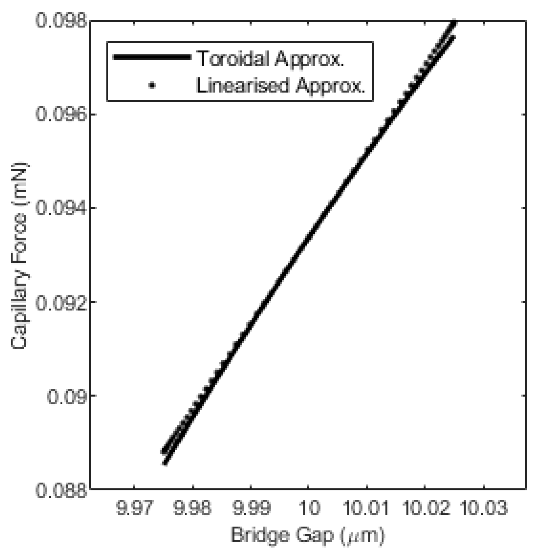
2.3. Linearization and Applicability to Squeeze Flow Rheometry

For this theory to be useful for squeeze flow rheometry, it is important that it is consistent with the fluid flow theory. In the fluid flow theory, it is assumed that the fluid has cylindrical geometry, the flow is purely radial, and that the no-slip condition applies [30]. These assumptions may seem to be at odds with the theory presented here. The reason for this is that, here, it is stated that the boundary is curved due to surface tension, precluding cylindrical geometry, and that the contact line can move, which will cause infinite shear stresses at the interface if the no-slip condition is applied and the flow is purely radial. This is because dealing with the exact boundary conditions in squeeze flow rheometry is not a trivial matter. This discrepancy is negated by ensuring that the lubrication approximation is applicable. The lubrication approximation states that if the fluid gap is much smaller than its radius, perturbations in the radial flow caused by edge effects can be neglected [17]. This means the individual force contributions from the surface tension and viscous flow can be treated separately and summed together [30].

One way to maintain consistency is to ensure the volume of liquid under consideration in the two theories is the same. To do this, the radius of fluid used in the fluid flow theory must be the root-mean-square of the radius of the bridge given in Equation (3), or:

$$RMS=\sqrt{\frac{1}{h}{{\displaystyle \int }}_0^{h}r{\left(z\right)}^{2}dz}$$

(17)

To see why this is consistent, recall that the volume of the bridge is defined as:

$$V={{\displaystyle \int }}_0^h\pi r{\left(z\right)}^{2}dz$$

(18)

And the volume of a cylinder with diameter $R_{Cyl}$ and height $h$ is defined as:

$$V=\pi R_{Cyl}^{2}h$$

(19)

If the definition of the root-mean-square radius, $RMS$, from Equation (17) is substituted into Equation (19) as the radius of the cylinder so that $R_{Cyl}=RMS$, it can be seen that Equations (18) and (19) are in fact the same (see Equation (10)).

$$V= \pi {\left(\sqrt{\frac{1}{h}{{\displaystyle \int }}_0^{h}r{\left(z\right)}^{2}dz}\right)}^{2}h={{\displaystyle \int }}_0^h\pi r{\left(z\right)}^{2}dz$$

(20)

Therefore, matching the $RMS$ value for the bridge radius does ensure that the volume of liquid used in both theories are consistent.

It was shown in [30] that if the capillary force can be described as a linear function then the equations of motion for a squeeze flow rheometer can be found. To linearise Equation (9), the change in the gap, $h$, must be sufficiently small as to not cause the contact line radius to slip. While the capillary force is still non-linear, if the change in gap is small enough, this nonlinearity will be small. This means the capillary force can be approximated by the linear relationship given in Equation (21), as demonstrated in Figure 13.

$$F_C\cong K_{Cap}x+{\chi }_{Cap}$$

(21)

The coefficients used in Equation (21) are:

$$K_{Cap}=\frac{d\left(F_C\left(\overline{h}\right)\right)}{d\overline{h}}$$

(22)

And:

$${\chi }_{Cap}=F_C\left(\overline{h}\right)-K_{Cap}\overline{h}$$

(23)

where $\overline{h}$ is the mean or nominal bridge gap. While these expressions are difficult to solve analytically, they are easily solved numerically. For instance, for the data shown in Figure 13, $K_{Cap}$ = 179.4 N/m and ${\chi }_{Cap}$ = −0.0017 N. The maximum relative error between the linear function given by Equation (21) and the data shown in Figure 13 is 0.11%. Therefore, Equation (21) can be used to determine the correction to the squeeze force measured during rheometry due to capillary forces and to check that these forces are linear, facilitating analysis of the rheometry data.

3. Conclusions

In this work, the geometry of a pendular liquid capillary bridge between two flat parallel platens has been determined, taking into account the contact angle hysteresis exhibited by the three-phase contact line of the bridge as the height of the bridge varies. The solution was based on the toroidal approximation, which is the assumption that the profile of the bridge is well approximated by a circular arc. This approximation has been extended for all contact angles from 0-180° for liquid bridges characterised by low Bond numbers. A closed form expression has been developed that allows for the fast approximation of the contact angle and contact radius at any bridge height without the need for significant experimentation or numerical analysis. All that is needed to be known before analysis is the bridge volume, the bridge height and the advancing and receding contact angles. This means that the effects of contact angle hysteresis, such as the resultant nonlinear capillary forces, can be calculated very conveniently whilst still maintaining accuracy. The inconsistency between the complex geometry of the liquid bridge and the simple geometry assumed during micro-squeeze flow rheology has been resolved, and the techniques for minimising the nonlinearities in the capillary forces during rheometry have been determined. The validity of the theory has been shown through comparison with the numerical solution of the exact governing equations.

References

1. Fowkes, F.M. Calculation of Work of Adhesion by Pair Potential Summatio. J. Colloid Int Sci. 1968, 28, 493–505. [Google Scholar] [CrossRef]
2. Allen, K.W. “At Forty Cometh Understanding”: A Review of Some Basics of Adhesion over the Past Four Decades. Int. J. Adhes. Adhes. 2003, 23, 87–93. [Google Scholar] [CrossRef]
3. Ennis, B.J.; Li, J.; Tardos, G.I.; Pfeffer, R. The Influence of Viscosity on the Strength of an Axially Strained Pendular Liquid Bridge. Chem. Eng. Sci. 1990, 45, 3071–3088. [Google Scholar] [CrossRef]
4. Simons, S.J.R.; Seville, J.P.K.; Adams, M.J. An Analysis of the Rupture Energy of Pendular Liquid Bridges. Chem. Eng. Sci. 1994, 49, 2331–2339. [Google Scholar] [CrossRef]
5. Rabinovich, Y.I.; Esayanur, M.S.; Moudgil, B.M. Capillary Forces between Two Spheres with a fixed Volume Liquid Bridge.: Theory and Experiment. Langmuir 2005, 21, 10992–10997. [Google Scholar] [CrossRef] [PubMed]
6. Lian, G.; Thornton, C.; Adams, M.J. A Theoretical Study of the Liquid Bridge Forces between Two Rigid Spherical Bodies. J. Colloid Int. Sci. 1993, 161, 138–147. [Google Scholar] [CrossRef]
7. Willett, C.D.; Adams, M.J.; Johnson, S.A.; Seville, J.P.K. Capillary Bridges between Two Spherical Bodies. Langmuir 2000, 16, 9396–9405. [Google Scholar] [CrossRef]
8. Pepin, X.; Rossetti, D.; Iveson, S.M.; Simons, S.J. Modelling the Evolution and Rupture of Pendular Liquid Bridges in the Presence of Large Wetting Hysteresis. J. Colloid Int. Sci. 2000, 232, 289–297. [Google Scholar] [CrossRef]
9. De Bisschop, F.R.E.; Rigole, W.J.L. A Physical Model for Liquid Capillary Bridges between Adsorptive Solid Spheres: The Nodoid of Plateau. J. Colloid Int. Sci. 1981, 88, 117–128. [Google Scholar] [CrossRef]
10. Orr, F.M.; Scriven, L.E.; Rivas, A.P. Pendular Rings between Solids: Meniscus Properties and Capillary Force. J. Fluid Mech. 1975, 67, 723–742. [Google Scholar] [CrossRef]
11. de Boer, M.P.; de Boer, P.C.T. Thermodynamics of Capillary Adhesion between Rough Surfaces. J. Colloid Int. Sci. 2007, 311, 171–185. [Google Scholar] [CrossRef] [PubMed]
12. Lambert, P.; Delchambre, A. Parameters Ruling Capillary Forces at the Submillimetric Scale. Langmuir 2005, 21, 9537–9543. [Google Scholar] [CrossRef] [PubMed]
13. Mastrangelo, C.H.; Hsu, C.H. Mechanical Stability and Adhesion of Microstructures under Capillary Forces: I. Basic Theory. 1993, 2, 33–43. [Google Scholar] [CrossRef]
14. Mastrangelo, C.H.; Hsu, C.H. Mechanical Stability and Adhesion of Microstructures under Capillary Forces: II. Basic Theory 1993, 2, 44–55. [Google Scholar] [CrossRef]
15. Mate, C.M. Application of Disjoining and Capillary Pressure to Liquid Lubricant Films in Magnetic Recording. J. Appl. Phys. 1992, 72, 3084–3090. [Google Scholar] [CrossRef]
16. Pfohl, T.; Mugele, F.; Seemann, R.; Herminghaus, S. Trends in Microfluidics with Complex Fluids. Chem. Phys. Chem. 2003, 4, 1291–1298. [Google Scholar] [CrossRef]
17. Bell, D.; Binding, D.M.; Walters, K. The Oscillatory Squeeze Flow Rheometer - Comprehensive Theory and a New Experimental Facility. Rheol. Acta 2005, 46, 111–121. [Google Scholar] [CrossRef]
18. Debbaut, B.; Thomas, K. Simulation and Analysis of Oscillatory Squeeze Flow. J. Non-Newton. Fluid Mech. 2004, 124, 77–91. [Google Scholar] [CrossRef]
19. Kwok, P.Y.; Weinberg, M.S.; Breuer, K.S. Fluid Effects in Vibrating Micromachined Structures. J. Microelectromech. Syst. 2005, 14, 770–781. [Google Scholar] [CrossRef]
20. Cheneler, D.; Bowen, J.; Ward, M.C.; Adams, M.J. Principles of a micro squeeze flow rheometer for the analysis of extremely small volumes of liquid. J. Micromech. Microeng. 2011, 21, 045030. [Google Scholar] [CrossRef]
21. Cheneler, D. Analysis of a Coupled-Mass Microrheometer. In Advances in Microfluidics; IntechOpen: London, UK, 2012; p. 55. [Google Scholar]
22. Yan, Y.; Zhang, Z.; Cheneler, D.; Stokes, J.R.; Adams, M.J. The influence of flow confinement on the rheological properties of complex fluids. Rheol. Acta 2010, 49, 255–266. [Google Scholar] [CrossRef]
23. Chen, T.-Y.; Tsamopoulos, J.A.; Good, R.J. Capillary Bridges between Parallel and Non-Parallel Surfaces and Their Stability. J. Colloid Int. Sci. 1992, 151, 49–69. [Google Scholar] [CrossRef]
24. Boucher, E.A.; Evans, M.J.B.; McGarry, S. Capillary Phenomena XX. Fluid Bridges between Horizontal Solid Plates in a Gravitation Field. J. Colloid Int. Sci. 1982, 89, 154–163. [Google Scholar] [CrossRef]
25. Concus, P.; Finn, R. Discontinuous Behaviour of Liquids between Parallel and Tilted Plates. Phys. Fluids 1998, 10, 39–44. [Google Scholar] [CrossRef] [Green Version]
26. De Souza, E.J.; Gao, L.; McCarthy, T.J.; Arzt, E.; Crosby, A.J. Effect of contact angle hysteresis on the measurement of capillary forces. Langmuir 2008, 24, 1391–1396. [Google Scholar] [CrossRef]
27. Shi, Z.; Zhang, Y.; Liu, M.; Hanaor, D.A.; Gan, Y. Dynamic contact angle hysteresis in liquid bridges. Colloids Surf. A Physicochem. Eng. Asp. 2018, 555, 365–371. [Google Scholar] [CrossRef] [Green Version]
28. Reynolds, O. On the Theory of Lubrication and Its Application to Mr. Beauchamp Tower’s Experiments, Including an Experimental Determination of the Viscosity of Olive Oil. Philos. Trans. R. Soc. Lond. 1886, 177, 157–234. [Google Scholar]
29. Borkar, A.; Tsamopoulos, J. Boundary-Layer Analysis of the Dynamics of Axisymmetric Capillary Bridges. Phys. Fluids A 1991, 3, 2866–2874. [Google Scholar] [CrossRef]
30. Cheneler, D.; Ward, M.C.; Adams, M.J.; Zhang, Z. Measurement of Dynamic Properties of Small Volumes of Fluid Using MEMS. Sens. Actuators B Chem. 2008, 130, 701–706. [Google Scholar] [CrossRef]
31. Neumann, A.W.; David, R.; Zuo, Y. Applied Surface Thermodynamics (Surfactant Science); CRC Press: New York, NY, USA, 1996; Volume 63. [Google Scholar]
32. Van Honschoten, J.W.; Tas, N.R.; Elwenspoek, M. The Profile of a Capillary Liquid Bridge Between Solid Surfaces. Am. J. Phys. 2010, 78, 277–286. [Google Scholar] [CrossRef]
33. Fisher, R.A. On the Capillary Forces in an Ideal Soil; Correction of Formulae given by WB Haines. J. Agric. Sci. 1926, 19, 492–505. [Google Scholar] [CrossRef]
34. Megias-Alguacil, D.; Gauckler, L.J. Accuracy of the toroidal approximation for the calculus of concave and convex liquid bridges between particles. Granular Matter. 2011, 13, 487–492. [Google Scholar] [CrossRef] [Green Version]
35. Willett, C.D.; Johnson, S.A.; Adams, M.J.; Seville, J.P.K. Pendular Capillary Bridges. In Handbook of Powder Technology: Granulation; Salman, A.D., Hounslow, M.J., Seville, J.P.K., Eds.; Elsevier B.V.: Amsterdam, The Netherlands, 2007; Volume 2, Chapter 28; pp. 1317–1351. ISBN 978-0-444-51871-2. [Google Scholar]
36. Blake, T.D. The Physics of Moving Wetting Lines. J. Colloid Int. Sci. 2006, 199, 1–13. [Google Scholar] [CrossRef]
37. Willett, C.D.; Adams, M.J.; Johnson, S.A.; Seville, J.P.K. Effects of Wetting Hysteresis on Pendular Liquid Bridges between Rigid Spheres. Powder Tech. 2003, 130, 63–69. [Google Scholar] [CrossRef]
38. Adams, M.J.; Johnson, S.A.; Seville, J.P.; Willett, C.D. Mapping the Influence of Gravity on Pendular Liquid Bridges between Rigid Spheres. Langmuir 2002, 18, 6180–6184. [Google Scholar] [CrossRef]
Figure 1. Schematic of the geometry of the liquid bridge.
Colloids 04 00013 g001
Figure 2. Schematic of the lower half of the liquid bridge denoting the various pressure and forces that result in the measured capillary force.
Colloids 04 00013 g002
Figure 3. Comparison between the geometry of the bridge profile as given by the numerical solution of the exact Laplace–Young equation (solid lines) and circular arcs representing the toroidal approximation (dashed line). The nondimensionalisation of the geometry is through the division by the cube root of the volume of the bridge.
Colloids 04 00013 g003
Figure 4. Schematic of the liquid bridge represented by the thick black line approximated with toroidal geometry.
Colloids 04 00013 g004
Figure 5. Schematic of the four stages of contact line motion during contact angle hysteresis.
Colloids 04 00013 g005
Figure 6. Schematic of the two extreme cases. Note that in both cases the contact line radii and volumes are equal. Only the gap between the platens and the contact angle have changed.
Colloids 04 00013 g006
Figure 7. Change in contact angle as a function of the normalised dimensionless gap. Each curve represents the result for a different dimensionless contact radius for the range of 1 to 3.
Colloids 04 00013 g007
Figure 8. Comparison of the coefficients generated as a result of the fit of Equation (16) to the contact angle as a function of the normalised dimensionless gap data shown in Figure 7 for increasing nondimensional contact radii and the functions given by Equation (17).
Colloids 04 00013 g008
Figure 9. Comparison between the approximate numerical answer and the closed form solution given by Equation (14) for R C * between 1 and 3.
Colloids 04 00013 g009
Figure 10. Capillary force hysteresis effects for a typical liquid bridge undergoing sinusoidal motion (the nominal gap is 10 µm amplitude is 1 µm, 3 × 101 nL and the Bond number is 0.0022) Left: the advancing contact angle is 70° and the receding contact angle is 20°. Right: the advancing contact angle is 140° and the receding contact angle is 70°.
Colloids 04 00013 g010
Figure 11. Variation of contact angle (left) and contact line radius (right) as a function of gap for the bridge detailed in Figure 10 (left).
Colloids 04 00013 g011
Figure 13. Linearised capillary force. Note that, as an example, the amplitude has been here reduced to 25 nm and, as a result, the contact radius is not able to slip, hence the capillary force is essentially linear.
Colloids 04 00013 g013