Prediction of Environment-Related Operation and Maintenance Events in Small Hydropower Plants

Abstract

Operation and maintenance (O&M) events resulting from environmental factors (e.g., precipitation, temperature, seasonality, and unexpected weather conditions) are among the primary sources of operating costs and downtime in run-of-river small hydropower plants (SHPs). This paper presents a data-driven methodology for predicting such long events using machine learning models trained on historical power production, weather radar, and forecast data. Case studies on two Slovenian SHPs with different structural designs and levels of automation demonstrate how environmental features—such as day of year, rain duration, cumulative amount of rain, and rolling precipitation sums—can be used to forecast long events or shutdowns. The proposed approach integrates probabilistic classification outputs with threshold-consistency smoothing to reduce noise and stabilize predictions. Several algorithms were tested—including Logistic Regression, Support Vector Machine (SVM), Random Forest, Gradient Boosting, and k-Nearest Neighbors (k-NN)—across varying feature combinations for O&M model development, with cross-validation ensuring robust evaluation. The models achieved an F1-score of up to 0.58 in SHP1 (k-NN), showing strong seasonality dependence, and up to 0.68 in SHP2 (Gradient Boosting). For SHP1, the best model (k-NN) correctly detected 36 long events, while 15 were misclassified as no events and 38 false alarms were produced. For SHP2, the best model (Gradient Boosting) correctly detected 69 long events, misclassified 23 as no events, and produced 42 false alarms. The findings highlight that probabilistic machine learning-based forecasting can effectively support predictive O&M planning, particularly for manually operated or service-operated SHPs.

1. Introduction

Small hydropower plants (SHPs) face unique operation and maintenance (O&M) challenges, particularly due to environmental variability such as precipitation, water flow rate, seasonality, and unexpected weather events due to global warming. O&M costs typically range from 1% to 5% of investment costs [1], but environment-related events (e.g., period of high water flow) can cause unplanned interventions, increased downtime, and higher expenses. Most of the O&M activities in an SHP [2] may be rescheduled to a more suitable time [3,4]; events related to the high water flow rates cannot be rescheduled without significant energy production loss. The time required for O&M activities can be up to ten times higher during periods of high water flow compared to stable environmental conditions [5]. Moreover, high water flow conditions often occur simultaneously in multiple SHPs, creating organizational challenges, which result in a suboptimal number of O&M personnel or increased O&M costs.

Environment-related O&M activities can be predicted with a certain probability in advance. These factors are particularly relevant for SHPs in torrential streams, which typically operate in mountainous (e.g., alpine) regions. Seasonal vegetation changes, rapid transitions from low to high water flow rates, sediment transport dynamics, water intake design, and susceptibility to sand and leaf blockages are among the most critical factors that complicate O&M prediction. A previous study [5] involving 86 SHPs operators found that the frequency of manual inspections varies significantly, ranging from once per week to five times per day.

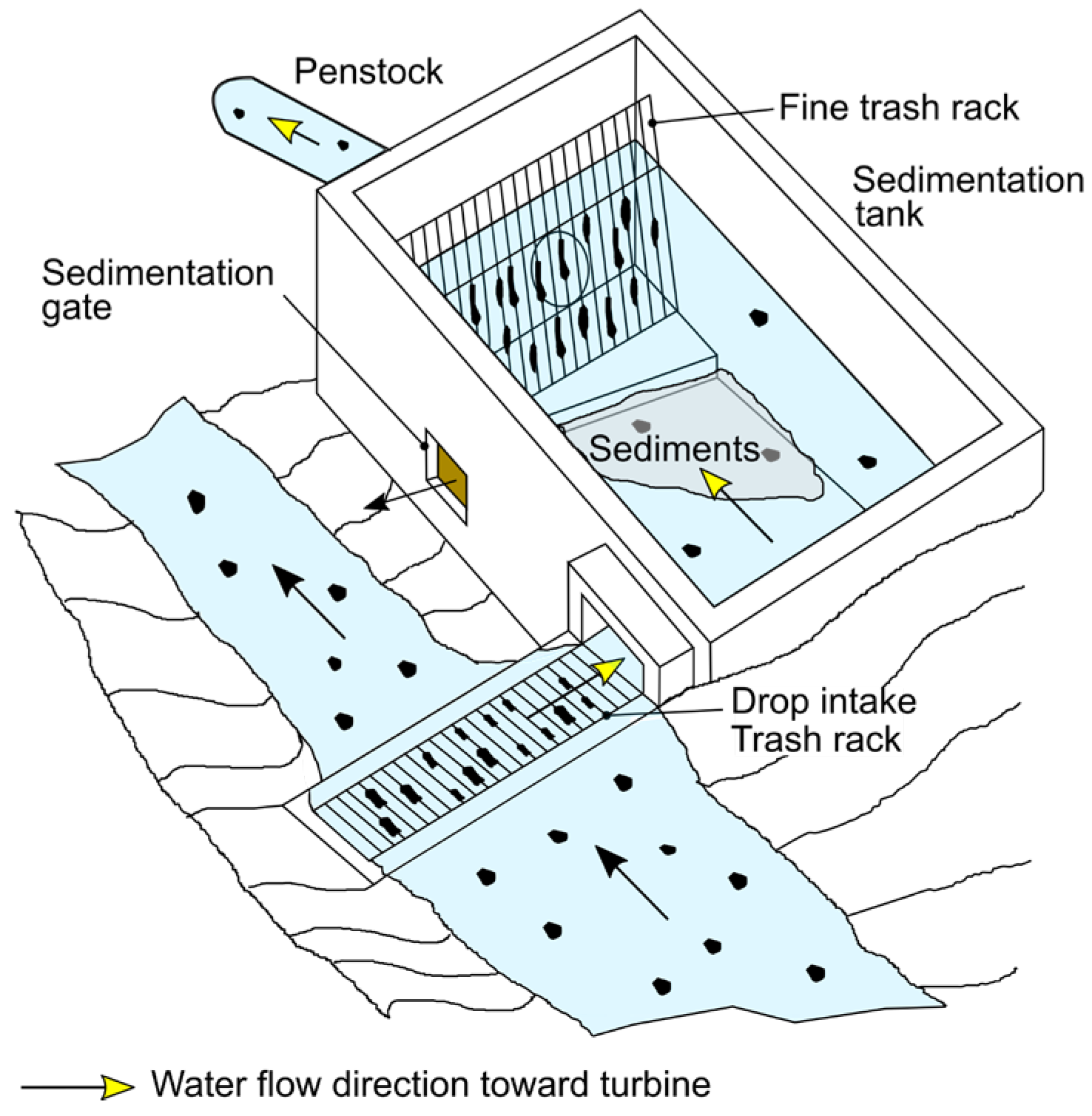
Run-of-river SHPs are the most common type of small hydropower plants. Their main components include a weir, a settling tank, a penstock, and a water turbine [6,7]. Water is diverted from the main river through an intake at the weir with minimal or no water stored in it. The intake features a trash rack designed to protect the turbines from large debris, including stones, timber, leaves, and man-made waste carried by the stream. Leaves and waste are filtered out at the trash racks, while sand settles in the settling tank (Figure 1). 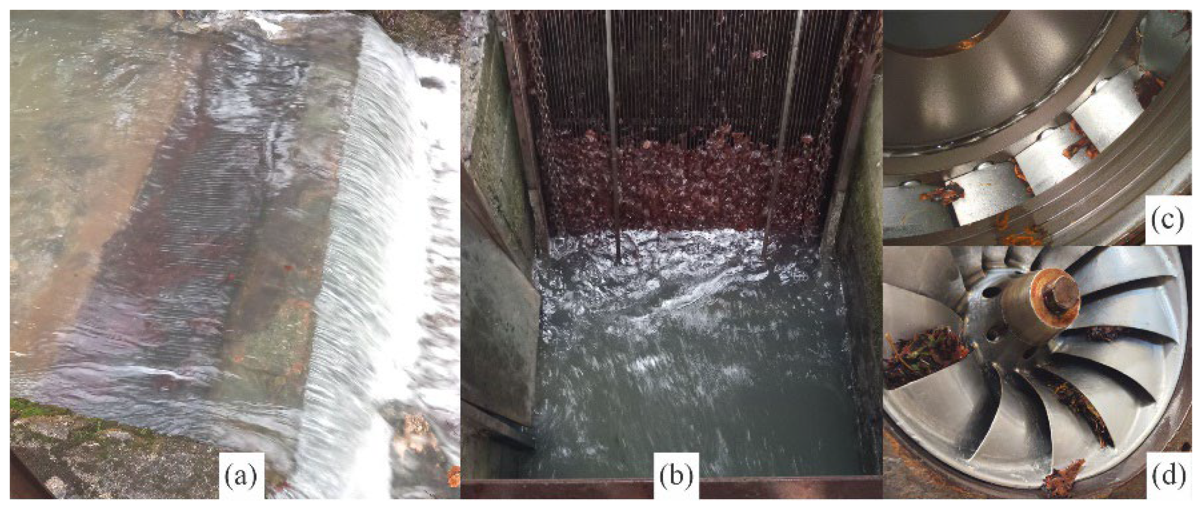For low head applications, the settling tank may be integrated into the stream or turbine intake [6]. The sand is released from the tank through the sedimentation gate. The trash racks are cleaned manually or with automated trash rack cleaning systems. Some particulate matter still enters the penstock, potentially causing clogging or turbine erosion. Smaller turbines are particularly susceptible to clogging by leaves. Representative examples of the operational challenges in SHPs are illustrated in Figure 2. The Tyrolean intake is partially clogged with leaves (Figure 2a), the main intake gate is entirely clogged with leaves (Figure 2b), and the guide vanes together with the Francis runner outlet gaps are partially blocked (Figure 2c,d). The trash rack clogging is related to the long events and stops, while turbine cleaning is related to short stops.

These operational problems are addressed mainly through manual intervention by the operator, or with some degree of automation and remote control. Manual interventions pose organizational challenges for operators or service providers, especially when they are responsible for many SHPs, since such interventions often require significant manpower at the same time.

Operational challenges observed in practice underscore the need to account for site-specific stream conditions already at the design stage of the SHP infrastructure. Engineers have developed guidelines for intake design [8] and the refurbishment of civil structures with an emphasis on silt management [9,10]. Barelli et al. [11] proposed a design approach for run-of-river SHPs that considers the hydrological characteristics of torrential streams.

To prevent turbine clogging due to leaves, self-cleaning turbine types may be used in SHPs as shown in the case of the Ossberrger crossflow turbine type [12]. A specialized guide vane cleaner was developed for very low head turbines [13]. In larger machines such as Kaplan turbines [14,15], the adjustability of guide vanes and runner blades can sometimes be exploited to increase flow and flush out leaves. In contrast, smaller turbines often rely on simple solutions such as dedicated access openings that allow operators to manually remove leaves and other debris. However, this process requires stopping the turbine, which can take up to a few hours. During autumn, such cleaning may need to be performed multiple times per week. Additionally, autumn leaves tend to be structurally robust and more prone to clogging the gates and turbine. By late autumn and early spring, the leaves break down into smaller fragments, allowing them to pass through the turbine more easily. Consequently, high water flow rates and leaf transport have a reduced impact on O&M events during these periods.

Given these dynamics, reliable detection of emerging O&M-related anomalies is essential for timely intervention. Online detection of O&M-related anomalies can be performed using classical statistical techniques for fault detection, such as control charts [16], change-point detection [17], or Bayesian monitoring approaches [18], as well as more advanced machine learning-based event classification models [19]. Machine learning offers advantages in handling nonlinear relationships, integrating multiple environmental variables, and learning complex temporal patterns directly from data.

In this paper, we address the problem of O&M events prediction using machine learning techniques. The primary focus is on long O&M events, which are mainly related to precipitation and allow for the prediction of these events a few hours in advance. We present an approach for SHP-specific O&M model generation based on past data. Based on forecasted data, this model offers operators probabilistic insights into whether a long event will occur in the next few hours. The O&M model is important for O&M personnel and service providers, which, especially at the beginning of service provision, lack insights into the SHP’s specific operations and river catchment characteristics.

The most problematic O&M events are related to the high water flow rate. However, systematic water flow monitoring and debris transport monitoring, especially in smaller rivers and streams, are not widely implemented. Moreover, while flow monitoring provides information about the actual flow rate in the river, it offers limited predictive capability for anticipating sudden inflow surges or debris-related blockages, which are critical for proactive maintenance and operational planning.

Most environment-related O&M activities in run-of-river SHPs are related to precipitation levels. Monitoring precipitation enables the prediction of water flow rates [20], as well as the associated debris transport. Sonnenborg [21] analyzed the value of different precipitation data for flood prediction in an alpine river basin. Traditionally, rain gauges have been used to measure precipitation. In recent years, radar-based rainfall monitoring has gained more attention due to its higher spatial and temporal resolution and greater areal coverage. Precipitation prediction in SHP is also crucial for production power forecasting [22], especially for the reservoir water management of hydropower plants [23,24].

Forecasting the peak water flow, which causes debris transportation in a stream, is a complex process. Both the spatial precipitation distribution, the characteristics of a river basin that affect overland runoff, and the characteristics of the stream channels impact the ability to generate reliable and useful forecasts. To simulate rainfall-runoff events, Jorgeson and Julien [25] developed a river basin model. The model was able to reproduce the peak flow and the time of the peak. This approach requires the calibration of the runoff model for each river basin area.

The main value of O&M prediction is to correctly and as far as possible in the future predict the start and duration of O&M events. This process is highly dependent on precise precipitation prediction. Weather models, both global and regional, are suitable for estimating precipitation a few days ahead. However, these models lack high horizontal resolution, particularly in small areas with irregular geographical features, complex orography, intricate coastlines, and heterogeneous terrestrial surfaces. For the geographical location of the SHPs in Slovenia, Ceglar et al. [26] developed a regional climate model. The model performed best in winter, when precipitation is primarily driven by large-scale processes. However, its performance was significantly lower in summer, when precipitation is predominantly caused by convective processes.

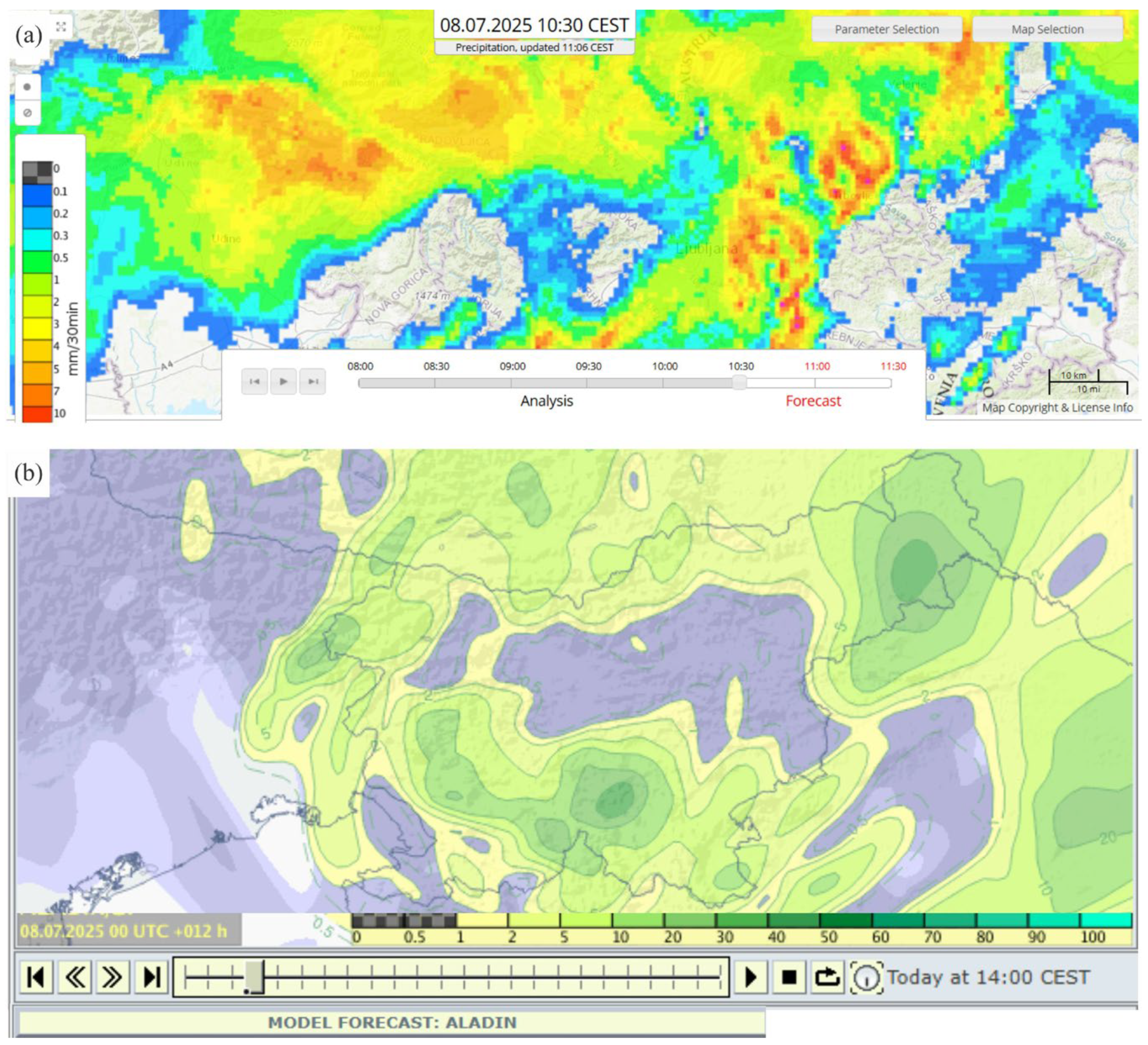
Analog methods and nowcasting are used for precipitation prediction over timeframes ranging from a few hours to a few days. An analog method for precipitation prediction involves analyzing historical weather data to identify patterns or situations that closely resemble the current meteorological conditions. Horton et al. [27] presented the genetic algorithm to optimize the analog method for precipitation prediction in the Swiss Alps. Nowcasting, on the other hand, utilizes data from weather station data, wind profiler data, and weather radar and satellite data to initialize current weather situations and to forecast by extrapolation for a period of a few hours. The implementation of nowcasting for the whole Central Europe domain has been established (Figure 3a). The nowcasting composite is calculated up to one hour in advance and is based on the INCA model, which was developed by the National Weather Service of Austria as part of the EU co-funded project INCA-CE [28].

In this study, the ALADIN (Aire Limitée Adaptation Dynamique Développement International) weather prediction model output is the primary meteorological input used in analyzing the forecasted precipitation. The weather model is a limited-area numerical weather prediction system developed by a consortium of European meteorological services led by Météo-France [29]. It is designed to downscale global model outputs to regional domains with finer spatial and temporal resolution (Figure 3b).

Precipitation prediction based on past weather data is an emerging research area. It increasingly leverages deep learning and neural networks, which utilize historical radar weather images to predict future precipitation [30,31]. These models are expected to improve in accuracy and geographic precision—an essential factor for the practical applicability of O&M prediction models. Deep learning approaches based on weather data have also been successfully applied to hydropower production forecasting [32].

Recent hydrological studies emphasize that runoff- and precipitation-driven processes are inherently nonlinear, exhibiting deterministic yet chaotic dynamics [33]. River flow depends on rainfall, soil saturation, and the underlying runoff model (deterministic behavior). However, depending on the season and the degree of catchment saturation, the same rainfall can trigger entirely different system responses—from high water levels and flooding to stable operation that does not necessarily lead to an event (chaotic behavior).

Based on the review of existing predictive O&M methods for small hydropower plants (SHPs), to the best of the authors’ knowledge, no existing approach provides a data-driven framework capable of predicting O&M events by jointly analyzing rainfall, multi-scale precipitation dynamics, and SHP behavior as a system. Existing studies typically focus either on hydrological forecasting or on turbine performance analysis, but do not integrate event-based rainfall–power relationships into a unified predictive model. Such rainfall–power relationships inherently include the effects of sediment transport processes and the sensitivity of the SHP system to debris and inflow dynamics, which can critically influence the occurrence and severity of O&M events.

This study develops O&M prediction models for SHP event forecasting using historical power production and environmental data, enhanced with forecasted environmental and precipitation-related features. O&M events are extracted from power production records, while precipitation features are derived from weather radar data specific to each river basin. Various machine learning algorithms are employed to generate O&M models, which are then evaluated, with the best-performing model selected for prediction.

The paper is organized as follows: Section 2 describes the methodology for O&M model generation and event prediction. Section 2.1 introduces case studies SHP1 and SHP2, along with the specific characteristics of their river basins. Section 3 presents the application and evaluation of the models for predicting O&M events in SHP1 and SHP2. Finally, Section 4 summarizes the key findings and outlines directions for future research.

2. Prediction Methodology and Data Preprocessing

2.1. Case Study SHPs

Throughout the paper, we refer to two small hydropower plants (SHPs), denoted as SHP1 and SHP2. These plants serve as case studies to present the methodology and its implementation demonstration. Since the SHPs are structurally different, certain variations in methodology implementation and results can be compared.

Both SHPs operate in a river basin located beneath the Blegoš mountain in Slovenia and share the same stream. They are run-of-river SHPs with a weir, penstock, and Francis-type turbines. SHP1 is equipped with a Tyrolean-type weir, whereas SHP2 employs a rubber dam with side water withdrawal. The installed flow capacity is 220 L/s for SHP1 and 280 L/s for SHP2. The maximum power production capacity is 70 kW for SHP1 and 60 kW for SHP2. On average, both SHPs generate a combined annual electricity output of approximately 900 MWh.

The operation of both SHPs is manual, including production power control. However, they are equipped with an auto-start function in the event of temporary unavailability of the electricity grid. Water intake and sedimentation gates are not automated. Both SHPs have trash rack cleaning machines, with SHP1 limited to a one-minute cleaning cycle and SHP2 to ten minutes. The drop intake gate in SHP1 is not equipped with a cleaning machine.

2.2. O&M Events Prediction Methodology

The predictive O&M model for O&M activities is developed using historical power production data and environmental parameters acquired in a synchronized manner. The methodology for forecasting O&M events comprises three distinct phases (Figure 4).

In the first phase, “dataset generation”, a training dataset is systematically constructed by integrating O&M event data derived from historical power production records with relevant environmental parameters extracted from archived environmental datasets. The goal is to be able to predict O&M events 72 h in advance. The probability of an O&M event occurring in the next 72 h, ${\tilde{p}}_{\mathrm{O}\&\mathrm{M}}$ can be expressed as a function of several attribute groups:

$${\tilde{p}}_{\mathrm{O}\&\mathrm{M}}=f(DM, PR,O\&M,D, RA)$$

(1)

where DM denotes directly measured environmental parameters, PR precipitation-related attributes, O&M are event-related attributes, D is time of year, and RA are relational attributes between DM, PR, O&M, and D. The full list of vector elements is provided in Section 2.6. This dataset serves as the foundation for model generation.

In the second phase, “training”, machine learning algorithms are applied to identify patterns and correlations within the data, enabling the generation of O&M predictive models. The trained models undergo a validation process to evaluate their predictive performance. The model demonstrating the highest predictive accuracy and generalization capability is selected for operational deployment.

In the third phase, “implementation”, the selected predictive model is integrated into SHPs operational workflows. The prediction horizon extends several hours into the future, contingent on the accuracy and reliability of the weather forecast data. The predicted probability ${\tilde{p}}_i$ at time i is expressed as a function of the selected O&M model and predicted DM_i, PR_i, O&M_i, D_i, and RA_i:

$${\tilde{p}}_{\mathrm{O}\&\mathrm{M}i}=f_{\mathrm{O}\&\mathrm{M}\_\mathrm{m}\mathrm{o}\mathrm{d}\mathrm{e}\mathrm{l}}\left({DM}_i,{PR}_i ,{O\&M}_i,D_i, {RA}_i\right)$$

(2)

The predicted O&M events are subsequently evaluated during real-time operation to assess the model’s predictive performance and practical applicability.

2.3. Precipitation Dataset Generation

The dataset consists of simultaneously acquired power production and environmental data over a period from 23 June 2018 to 12 April 2025. Despite the seven-year observation window, the dataset includes relatively few long events after filtering. This reduces statistical robustness and is an inherent limitation of the study.

Precipitation measurements were collected from the WRM-200 weather radar, which provides 10 min interval radar images in GIF and GRIB formats. For the eleven most intensive rainy periods from August 2024 to April 2025, the regional ALADIN forecast data (GRIB format) were obtained as well. Each ALADIN model is run every six hours and ranges for 72 h in advance. Between these two models, another prediction is run which ranges 36 h in advance. Additional environmental parameters, including snow height, wind speed, temperature, and water flow rate, were sourced from the Slovenian Environment agency’s measuring stations [34]. Power production data from SHP1 and SHP2 were collected from the Slovenian electricity distribution system operator website [35], with access granted by the SHP’s owners.

The most important environmental parameters were calculated from the precipitation data. In mountainous areas, precipitation is highly localized, requiring individual calculations for each river basin to determine the total rainfall. Weather radar data provide 1 km of spatial distribution, which is often too coarse for mountainous regions. As a result, a river basin associated with an SHP may have only one or two calculation points. The ALADIN weather forecast has an even lower spatial resolution of 4.3 km.

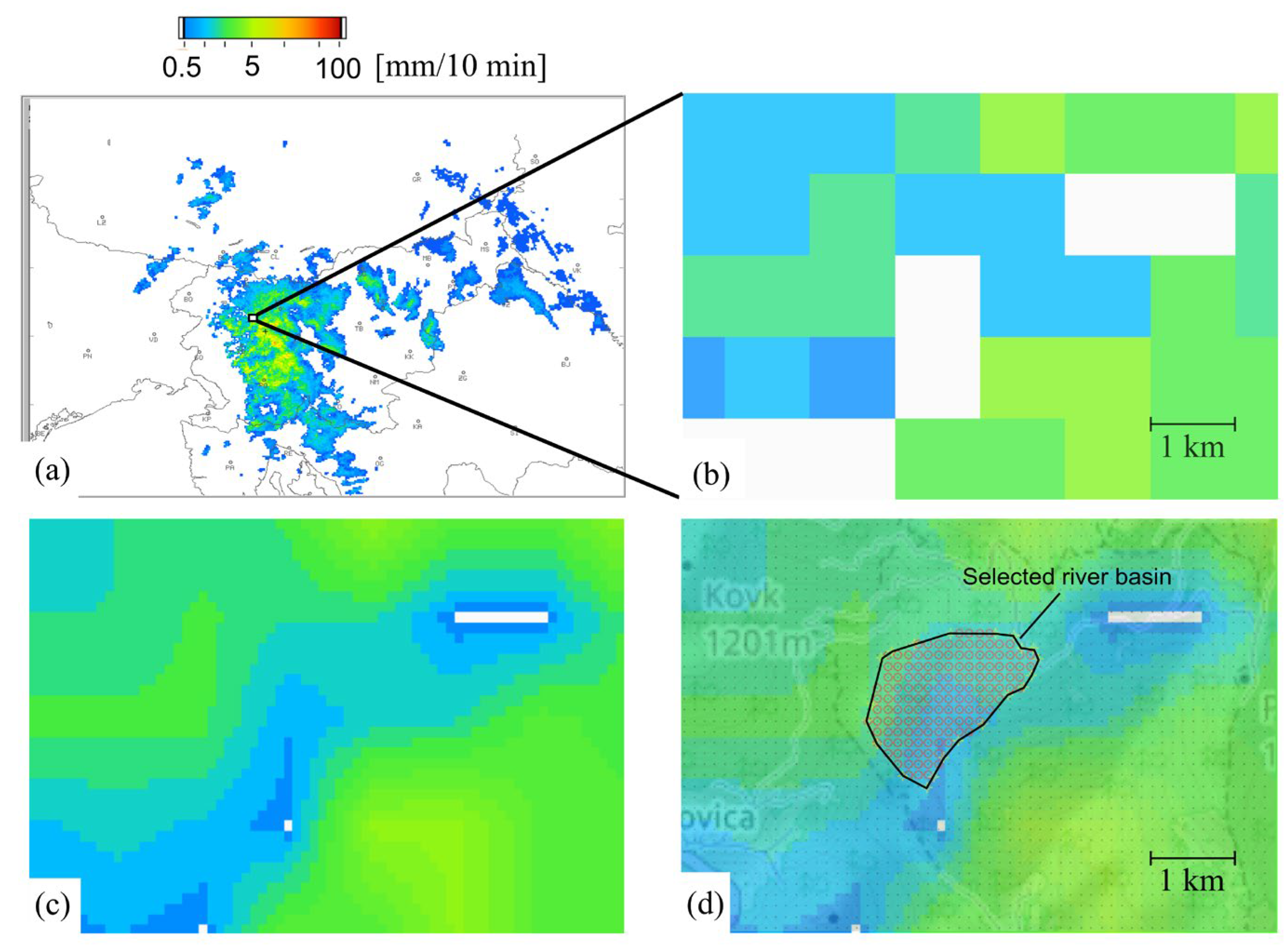
The process of calculating rainfall from weather radar precipitation data is illustrated in Figure 5. It shows precipitation measurements obtained from radar, where the color scale represents the rainfall intensity per square kilometer over a 10 min interval. To analyze a specific river basin, a region of interest is selected (Figure 5b). Due to the low resolution between radar measurement points, linear interpolation is applied between two radar calculation points (Figure 5c). The precipitation data are then mapped onto a grid over terrestrial maps (Figure 5d), allowing for the precise identification of river basins. The border polygon of the river basin was selected as the WGS84 polygon for each SHP, individually. When defining the river basin, factors such as mountain crests, watershed boundaries, and existing watercourses must be considered. Once the river catchment area is selected, the total rainfall for the area over a 10 min interval, denoted as r_i, is calculated.

From the precipitation data, the total amount of rain A_p is calculated as follows:

$$A_{\mathrm{P}}={\sum }_{t_{1R}}^{t_{2R}}{r}_i$$

(3)

where $t_{1R}$ and $t_{2R}$ denote the start and end times of rainfall, respectively, and $r_i$ is the precipitation rate in mm/10 min at the i-th time interval.

The calculation procedure was applied to the radar images. For ALADIN forecasts the procedure was similar, considering lower spatial and temporal resolution. To ensure spatial consistency, the same WGS84 polygon used for the radar images was also applied to the ALADIN forecasts.

2.4. O&M Events

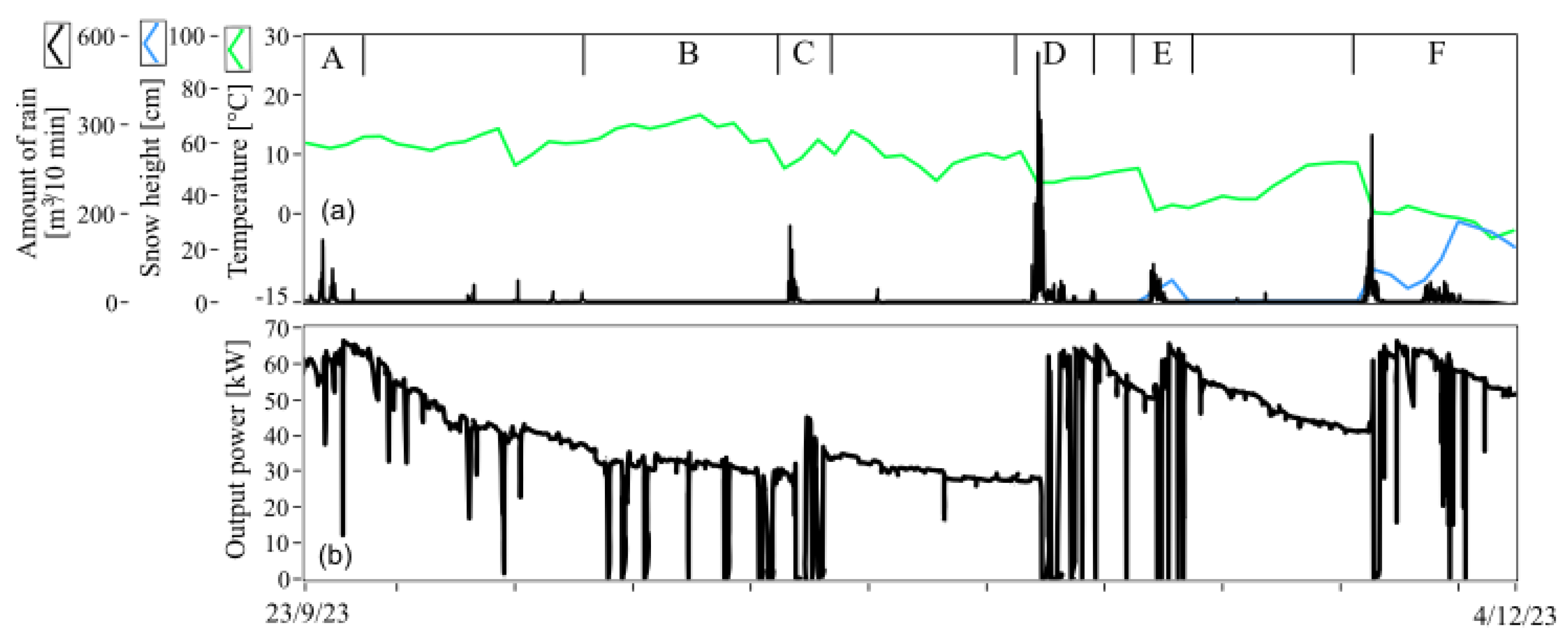
High-priority O&M events in a run-of-river SHP are closely related to the environmental conditions (Figure 6). Figure 6a shows measured environmental data, while Figure 6b presents the measured power production data for SHP1. The plotted data for approximately two months coincide with the autumn season, which is characterized by leaf fall and rainy periods. If the output power dropped to zero, the SHP was stopped, triggering an O&M activity. The O&M events in periods A, C, D, E, and F are related to precipitation, whereas period B events correspond to the leaf fall period. In period A, precipitation did not cause operational problems resulting in stops. Period B is characterized by frequent stops due to trash rack blockages caused by leaves. In period C, precipitation caused an immediate stop of the SHP. This stop resulted from leaf transportation and trash rack blockage. In this case, due to the previous dry period, the operational power did not increase. The rainy periods D and E both caused stops. In these periods, the operational power increased, which indicates that the water flow increased. A higher water flow rate caused flushing of leaves from the riverbank and sand transportation, both of which triggered O&M activities. In period F, the number of stops decreased. During this time, snow covered the remaining leaves on the surface, and most of the leaves had been flushed from the riverbank, resulting in fewer stops and reduced operational problems. Considering the amount of precipitation and its temporal distribution, it may be possible to predict the stop of the SHP.

2.5. O&M Event Generation from Past Power Production Related Data

The basic O&M events that require the presence of the operator in the SHP include a long stop, a gradual event, and a short stop. These events are identified from the power production signal (Figure 7). Three types of algorithms are used to detect different O&M event types.

The first algorithm detects long events (Figure 7a), which typically coincide with high water flow rates or sedimentation tank cleaning. The second algorithm identifies gradual events (Figure 7b), characterized by a gradual decline in power production. These events result from the intake trash rack blockages, particularly during the autumn leaf fall period when leaf accumulation is most intensive. After the operator manually cleans the trash rack, power production automatically returns to its nominal level. The third type of algorithm detects short stops (Figure 7c). These events indicate turbine cleaning, which is a consequence of the turbine clogging with leaves.

The start of the event (t₁), the end of the event (t₂), and the length of the event (t_e) are the most important attributes describing O&M events. Time duration (t_d) separates the long and short events. If t_e > t_d, then the power signal is classified as a long event (Figure 6a); if t_e < t_d, the signal is classified as a short event. If the power gradient P_g is within a predetermined range, a gradual event is detected. The attributes t_d and P_g are determined based on expert knowledge for each SHP individually.

Gradual events are a consequence of both environment-related phenomena as well as operating procedures and the level of SHP automation. Gradual events may sometimes indicate not only trash rack blockage but also, for example, the presence of air gaps in the penstock. The latter is related to power production control, which may be remotely or automatically controlled. Therefore, gradual events are excluded from prediction modeling.

Short events are primarily related to turbine cleaning, which mostly occurs in autumn during the leaf fall period. The need for cleaning can also be detected through remote monitoring and, if necessary, postponed for a few days at the cost of a small loss in energy production. Therefore, short events are also excluded from prediction modeling.

Long events that coincide with rainfall cannot be postponed and may even pose safety risks, making them the primary focus of this study. Long events lasting several hours, such as sedimentation cleaning or other maintenance activities occurring outside rainfall periods, are excluded from the modeling.

Figure 8 shows the events and the corresponding rainfall and duration over an eight-year period in SHP1. Since long events might be several times longer than short events, a logarithmic scale is used to denote event duration. Most of the events occurred during the second half of a year and during autumn, which correspond to leaf fall and high water flow rate periods.

The average number and duration of events at SHP1 and SHP2 is summarized in

Table 1. Number and duration of events per year in the case of SHP1 and SHP2, calculated as average per 8 years.

	Short Events		Gradual Events	Long Events		Long Events During Raining
	Nr. of Events	Total Duration [h]	Nr. of Events	Nr. of Events	Total Duration [h]	Nr. of Events
SHP2	26	8	5	15	136	24
SHP1	22	15	18	14	111	16

. The annual occurrence of short and long events is similar between the two sites. At SHP2, 26 short events occur per year, while SHP1 experiences 22. Long events are less frequent, with SHP2 averaging 15 per year and SHP1 averaging 14. Despite being fewer in number, long events have a greater total duration than short events. At SHP2, long events accumulate to 136 h annually, compared to 111 h at SHP1. A notable difference between the two SHPs is the frequency of gradual events: SHP2 records 5 gradual events per year, whereas SHP1 experiences 18. This disparity is due to the lack of a trash rack mechanism at the drop intake of the Tyrolean weir at SHP1 and the higher turbine susceptibility of being clogged by leaves.

The results were derived from both algorithmically identified and manually verified events. When relying solely on algorithmic identification of long events occurring during rainfall, the annual frequency increased slightly, yielding 24 and 16 long events per year for SHP2 and SHP1, respectively.

2.6. Datasets for Various O&M Prediction Hypotheses

This study focuses on O&M prediction model generation primarily based on precipitation data and relationships with the O&M events listed in

Table 2. The key features for O&M event prediction model generation.

	Directly Measured (DM)	Precipitation Related (PR)	O&M Events Related (O&M)	Date	Relational Attribute (RA)
O&M-related parameters	Snow height [cm] Temperature [°C] Wind speed [m/s] Water flow rate [m3/s]	Start of rainfall [DOY–hh:mm] End of rainfall [DOY–hh:mm] Duration of rainfall Amount of rain [m3] Rolling sum of precipitation [m3/period] Maximum rolling precipitation intensity [m3/period]	Time from start of event to end of event [s] Time after the previous event [s]	Time of year [DOY]	Duration of rainfall to the event [s] Time from the start of snow melting to the event [s] Time from start of windy conditions to the event [s] Time from the occurrence of the maximum raining intensity to the event [s] Water flow rate determined from power production at the time of event [m3/s]

. The list was conducted with the help of SHPs operators. Table 2 categorizes the features into five main groups: directly measured parameters (DM), precipitation-related attributes (PM), O&M event-related parameters (O&M), date, and relational attributes (RA). The listed features reflect operator experience regarding factors that influence O&M events, although not all of them are technically suitable for O&M modeling. For example, conditions such as above-zero temperatures, snowmelt in mountains, and moderate rainfall can lead to increased water flow that triggers O&M activity. However, measuring snow height requires a dedicated measurement station at each SHP site and long-term data collection to build a robust dataset. Due to these limitations, some features were excluded from the modeling.

2.7. Long Event- and No Event-Related Features

The long event was calculated as described in Section 2.5. From the power production, the start of the long event and duration of the long event were calculated. In the case of no_event, the end of rainfall is equalized with the start of the event (t₁ = t_2R). For both events, only the relevant features from Table 2 were calculated (Figure 9): day_of_year, cumulative_amount_of_rain, rain_duration, and rolling_amount_of_rain for the last 1 h, 3 h, 6 h, and 9 h. To support the hypothesis about leaf flushing, additional features were calculated: power_production at the start of the event, the last_maximum_rolling_precipitation_intensity, and time_from_last maximum_rolling_precipitation_intensity. The preprocessing algorithm for event detection and feature extraction is provided in Appendix A.

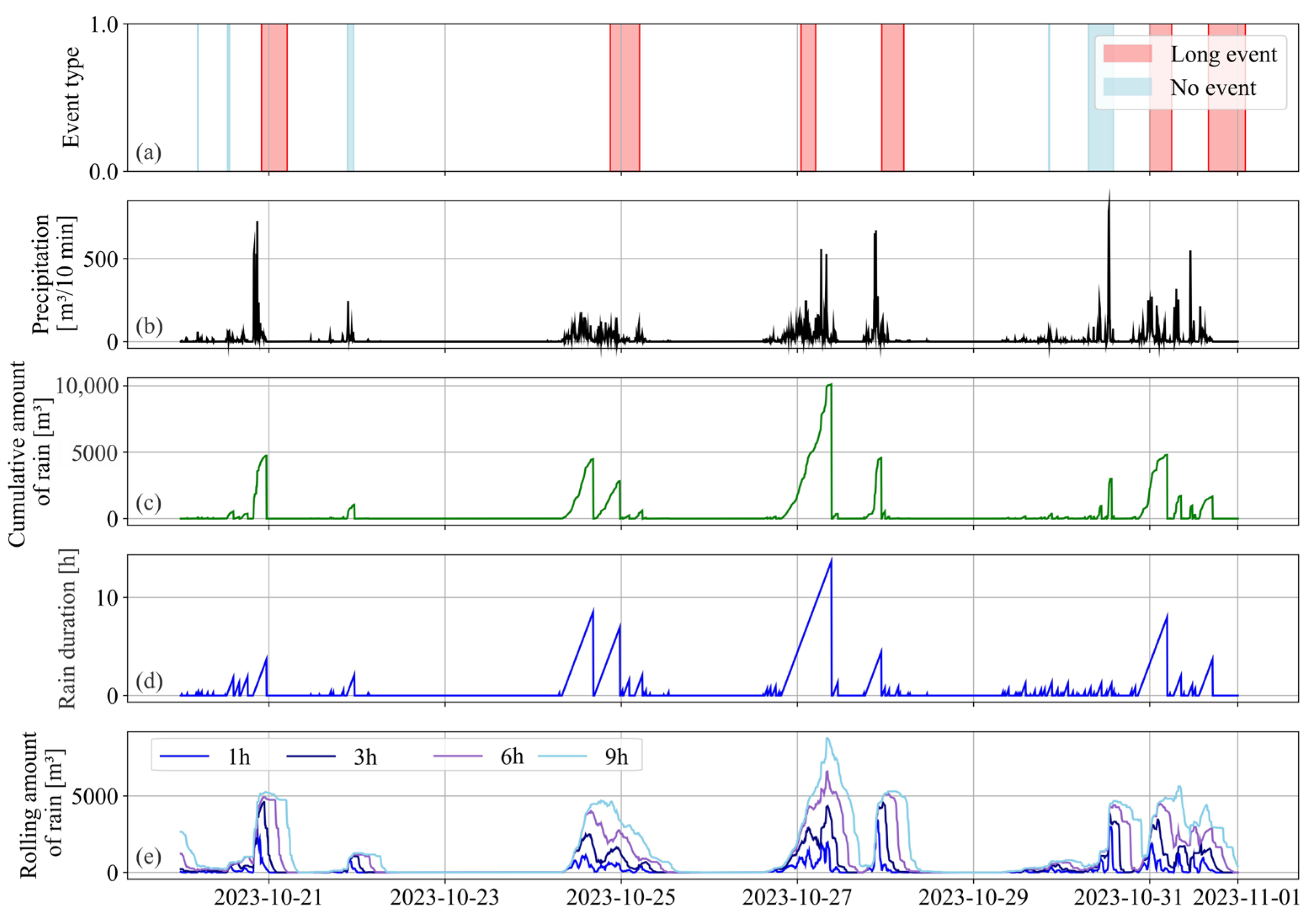
Figure 10a shows the detected events along with the corresponding feature values over time. The red shading shows the period of long events; the blue shading shows the raining period, which did not result in long event. Figure 10b shows the temporal distribution of precipitation. Figure 10c–e show the feature values calculated from Figure 10a,b as explained in Figure 9. A higher feature value corresponds to an increased probability of long event occurrence. Figure 10c,d reveals a strong relationship between the cumulative amount of rain and rain duration and the likelihood of a long event. Therefore, we calculate the parameter rain intensity, which is used for visual representation of data.

$$Rain intensity={\displaystyle \frac{Cumulative amount of rain}{Rain duration}}$$

(4)

In the algorithm, the start and end of the raining period is parametrically defined using a threshold. This threshold directly influences the calculated rain duration, which can vary significantly depending on its value. In contrast, the rolling amount of rain (Figure 10e), which is calculated over the preceding 1, 3, 6, or 9 h, is not defined with the threshold parameter and is therefore a more reliable feature. Furthermore, these rolling features can also support the prediction of the event’s end, as water level typically takes time to recede below a certain operational threshold.

To evaluate the impact of various parameters on O&M event prediction, two datasets were developed, as shown in

Table 3. Datasets for O&M prediction model training.

Feature Nr.	Dataset	Parameter	Prediction Hypothesis
1	1	Day of year [DOY]	Events based on the day of the year are predicted.
2	1	Cumulative amount of rain [m3]	Event starts influenced by rainfall are predicted.
3	1	Rain duration [s]	Rain duration enhances the model by improving event start prediction.
4–6	1	Rolling amount of rain in 1, 3, 9 h [m3]	The rolling sum of precipitation improves the prediction of event start and end times.
7	2	Maximum rolling intensity [m3/10 min]	It may indicate the leaves flushing from the riverbanks.
8	2	Time from last maximum rolling intensity [s]	Long time after maximum rolling intensity may indicate more leaves present in the riverbanks (e.g., due to the windy conditions).
9	2	Power production [kW]	Production power serves as an indirect indicator of water flow, reflecting watershed wetness and runoff dynamics.

. Dataset 1 predicts operational stoppages based on the day of the year, the cumulative amount of rain, and rain duration, capturing seasonal variations and the start of the event. Dataset 1 also includes a rolling sum of precipitation and duration of event, which improves the prediction of event start and event end times. In dataset 2, maximum rolling intensity, time from last maximum rolling intensity, and power production might better predict events related with leaf accumulation, sand transportation, and leaf flushing from the riverbanks. The operating power parameter proved to be problematic for reliable river flow estimation, as it can vary during rainfall periods. Therefore, this parameter was excluded from the analysis. The optimal set of features for O&M model generation may differ for each SHP. To determine the most relevant parameters for each SHP, feature importance metrics are calculated.

2.8. Event Prediction Features

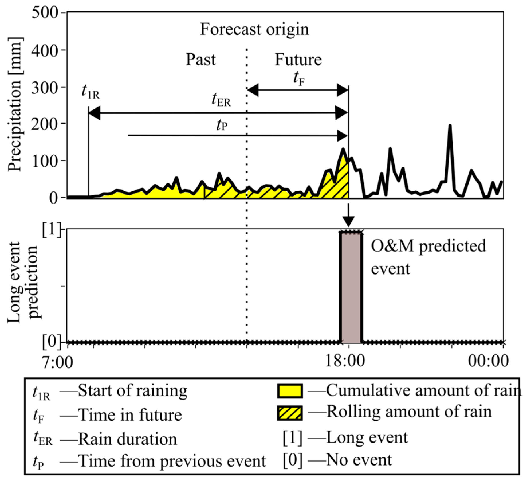
To predict O&M events, the same parameters used during O&M model training must be recalculated using both past and forecasted precipitation data. Past rainfall information is derived from radar images, while future precipitation is based on ALADIN forecasts, following the precipitation calculation methodology outlined in Section 2.3. For each forecast time step, t_F, the features listed in Table 2 are computed (see Figure 11). These calculated features are then input into the trained O&M prediction model, allowing it to estimate the probability of upcoming O&M events.

3. Predictive Modeling and Event Forecasting

3.1. O&M Prediction Model Metrics

The O&M prediction model utilizes multidimensional learning algorithms capable of effectively classifying attributes that may initially seem unrelated. To select the best machine learning algorithm, the decision metrics are calculated. For example, the confusion matrix provides a clear assessment of the model’s classification performance in the context of O&M prediction (Figure 12).

The rows of the confusion matrix represent the true event classes, while the columns indicate the predicted classes. The sum of the elements in each row corresponds to the total number of events for each class. Diagonal elements denote correctly predicted events. Off-diagonal elements indicate misclassified events, referred to as incorrectly predicted events. For example, shown in Figure 12, in the case of long events, the model correctly predicts five long events, while misclassifying five events as no event and two as long events. From the operator’s perspective, the O&M prediction model is incorrect (1) if the model predicts O&M activity, but it is not necessary to make it (false positive), and (2) if the model predicts no event but the operator’s intervention is required (false negative). The first case causes unnecessary O&M expenses arising from visiting the SHP, and in the second case the operator missed a critical event. Thus, accurate prediction of true long events is particularly critical, as misclassification in this category can lead to significant operational risks.

To evaluate the model from a long event perspective, four parameters from the confusion matrix are calculated: (1) overall classification accuracy, (2) precision, (3) recall, and (4) F1-score. Firstly, we define true positives (TPs), which are correctly predicted instances for each class, false positives (FPs), incorrectly predicted instances for each class, and false negatives (FNs), actual class, but predicted as something else. For the case shown in Figure 13, the TP(no_event) is 103, TP(long_event) is 5 (true no_event, predicted no_event), FP is 5 (predicted no_event, actually long_event), and FN is 2 (predicted long_event, actually no_event).

Accuracy is defined as the proportion of correct predictions against total predictions.

$$Accuracy={\displaystyle \frac{Correct prediction}{Total predictions}}$$

(5)

The classification model correctly identified 103 instances of the no_event class and 5 instances of the long_event class, resulting in a total of 108 correct predictions out of 115 instances. Given that there were 105 no_event and 10 long_event instances, the overall classification accuracy is 108/115 = 0.939, or 93.9%. Accuracy gives equal weight to all classes, but in practice missing a long_event is far more critical than falsely detecting no event. Thus, the accuracy does not tell if the model is better at detecting one class than another.

To obtain a more complete picture, the precision is calculated. Precision gives an answer, out of all predicted instances of a class, as to how many were correct.

$$Precision={\displaystyle \frac{TP}{TP+FP}}$$

(6)

For the long_event class, precision is 5/(5 + 2) = 0.714

Recall (sensitivity) gives an answer, out of all actual instances of a class, as to how many the model correctly identified.

$$Recall={\displaystyle \frac{TP}{TP+FN}}$$

(7)

For the long_event class, the recall is 5/(5 + 5) = 0.500

F1-score is a harmonic mean between precision and recall.

$$F1=2\cdot {\displaystyle \frac{Precision\cdot Recall}{Precision+Recal}}$$

(8)

The F1-score is 2 × (0.714 × 0.500)/(0.714 + 0.500) = 0.588. The F1-score is the most important metric since it gives the balance between precision and recall. Therefore, the F1-score was selected to choose the best classification algorithm.

3.2. Machine Learning Algorithms

In this study, several machine learning algorithms were employed for O&M model generation. The chosen algorithms include Logistic Regression, Support Vector Machine (SVM), Random Forest, Gradient Boosting, and k-Nearest Neighbors (k-NN). These algorithms cover a spectrum from simple linear models to powerful ensemble methods and non-parametric approaches, allowing us to compare their performance across data from both SHPs. All the classifications were made using the scikit-learn machine learning library (version 1.2.2) implemented in Python 3.10 [36]. Below is a detailed description of the configurations used for each model.

For all models—except k-NN, which does not support class weighting in scikit-learn—a class weight of {1:3} was applied to address class imbalance, giving greater importance to the less dominant long_event class. For hyperparameter selection, a grid search procedure was employed, and the parameters yielding the highest F1-score were used for the learning models configurations (

Table 4. Machine learning models and configurations.

Model	Configuration
Logistic Regression	Maximum iterations = 1000 (ensures convergence); class_weight = {0:1, 1:3}. Serves as a linear benchmark model.
Support Vector Machine (SVM)	Polynomial kernel (degree = 3); regularization parameter C = 15 (balance between bias and variance); automatic scaling of kernel coefficient, class_weight = {0:1, 1:3}.
Random Forest	70 estimators (trees); maximum depth = 5; minimum samples per leaf = 50; maximum features per split = square root of total number of features, class_weight = {0:1, 1:3}.
Gradient Boosting	100 boosting iterations; learning rate = 0.1; maximum 31 leaf nodes per tree; minimum 20 samples per leaf; up to 255 histogram bins; class_weight = {0:1, 1:3}. The latest scikit-learn library provides this algorithm under the name HistGradientBoosting.
k-Nearest Neighbors (k-NN)	k = 15; prediction based on the vote of 15 nearest neighbors with equal weights; Euclidean distance (p = 2); automatic search algorithm; default leaf size = 30; sensitive to density and distribution of nearby points.

).

These configurations aim to balance model complexity and generalization, while minimizing the risk of overfitting. Data preprocessing involved scaling to normalize the input features before feeding them into the model. Additionally, all models include probability estimation, allowing for probabilistic classification outputs.

3.3. Event Probability Calculation

In machine learning classification, the event probability is typically the model’s predicted likelihood that a given input x belongs to the positive class (long event). The general formulation is as follows:

P(y = 1|x) = f(x)

(9)

where x = (x₁, x₂, …, xₙ) is the feature vector (e.g., features from Table 3), y ∈ {0, 1} is the class label, where y = 1 denotes a long event, and f(x) ∈ [0, 1] is the predicted probability.

Each classification algorithm uses a model-specific probability function [30]:

-

Logistic Regression:

f(x) = 1/(1 + exp(−(w ^Tx + b)))

(10)

where w is the weight vector learned from the data and b is the bias.

-

SVM:

f(x) = 1/(1 + exp(A g(x) + B)),

(11)

where g(x) is the SVM decision function, and A,B are calibration parameters estimated via Platt scaling [37].

-

Random Forest/Gradient Boosting:

$$f\left(\mathit{x}\right)={\displaystyle \frac{1}{M}}{\sum }_{m=1}^M{h}_m\left(\mathit{x}\right),$$

(12)

where hₘ(x) ∈ [0, 1] is the probability predicted by the m-th decision tree, and M is the total number of trees [38].

-

k-Nearest Neighbors (k-NN):

f(x) = (1/k) ∑_i I(y_i = 1),

(13)

where yᵢ are the labels of the k nearest neighbors of x and I[] is the indicator function [38].

For each time step t, the probability of a long_event was computed as follows:

$$P(yₜ = 1 | \mathit{x}ₜ) = f(\mathit{x}ₜ)$$

(14)

These probabilities were then thresholded to produce binary event predictions.

3.4. Threshold-Based Probability Calculation

In contrast to using the raw output probability from a classification model, a threshold-consistency approach [39] can be used to compute a smooth and more robust estimate of event probability. This method evaluates how consistently the model predicts a long event across a range of decision thresholds.

Let pᵢ be the raw predicted probability at time step i, and let T = {t₁, t₂, …, t_k} be a predefined set of decision thresholds (e.g., from 0.1 to 0.9). The threshold-consistency-based event probability at time i, denoted as ${\tilde{p}}_i$, is defined as follows:

$$\tilde{p}\mathrm{ᵢ}= {\displaystyle \frac{1}{k}}{\sum }_{j=1}^{k}I\left(p\mathrm{ᵢ} \ge tₖ\right)$$

(15)

where I() is the indicator function, returning 1 if the condition is true and 0 otherwise, and k is the total number of thresholds. This approach effectively measures the proportion of thresholds that the raw probability exceeds. It smooths out local noise and provides a normalized measure of prediction confidence. A higher value of ${\tilde{p}}_i$ indicates that the model is consistently confident in predicting a long event at time i, while lower values suggest uncertainty or threshold sensitivity.

The methodology outlined in Section 2 was applied to operational and environmental data from SHP1 and SHP2 to evaluate the feasibility and performance of the O&M prediction models. The following section presents the results of the model training, evaluation, and analysis of prediction performance.

4. Results and Evaluation

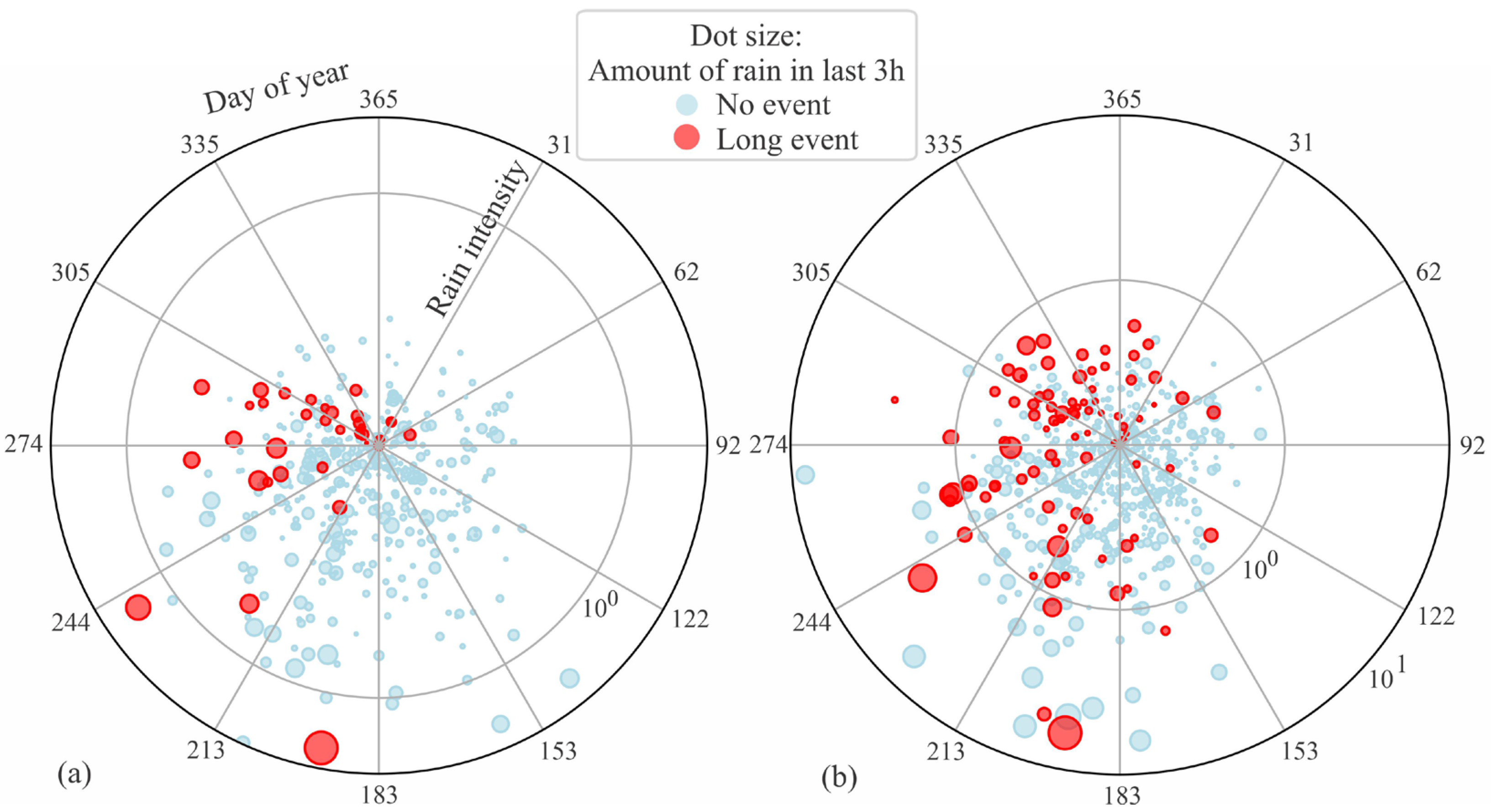
The average yearly precipitation distribution in SHP1 and SHP2 is shown in Figure 13. In total, in SHP1 there were 520 no_events and 51 long_events. In SHP2, there were 756 no_events and 92 long_events. In SHP1, most events occur in autumn. In other seasons, long events are typically triggered only when rainfall is substantial. However, some periods of intense rainfall do not result in events, while in autumn, even a small amount of rain can cause a long event. In SHP2, the seasonal distribution is relatively uniform from July to March, but there is a concentration of events during the summer months, where high-intensity rainfall leads to more frequent shutdowns compared to SHP1.

Most of the events in both SHPs are related to the leaf fall. The river catchment height for both SHPs ranges from 600 to 800 m. In the Alps, for this height, the autumn period starts in late September (25 September—day 268), peaks in the middle of October (15 October—day 288), and ends at the beginning of November (November 10, day 314). However, tree species, slope orientation, and microclimate may affect the exact start and intensity of leaf fall. Leaves from Acer fall earlier compared to Fagus, the dry season triggers leaves to fall earlier, and the freezing temperature and windy conditions may intensify the leaf fall. This results in substantial leaf fall variation periods and intensities, which also affect the events’ probability.

4.1. Feature Importance for SHP1 and SHP2

Initially, the Random Forest algorithm was applied for O&M model generation. The dataset was randomly shuffled, and to address class imbalance a weighting scheme of 1:3 was applied, giving higher importance to the long_event class. Model performance was evaluated using 5-fold stratified cross-validation, ensuring that each event was used once for testing and four times for training.

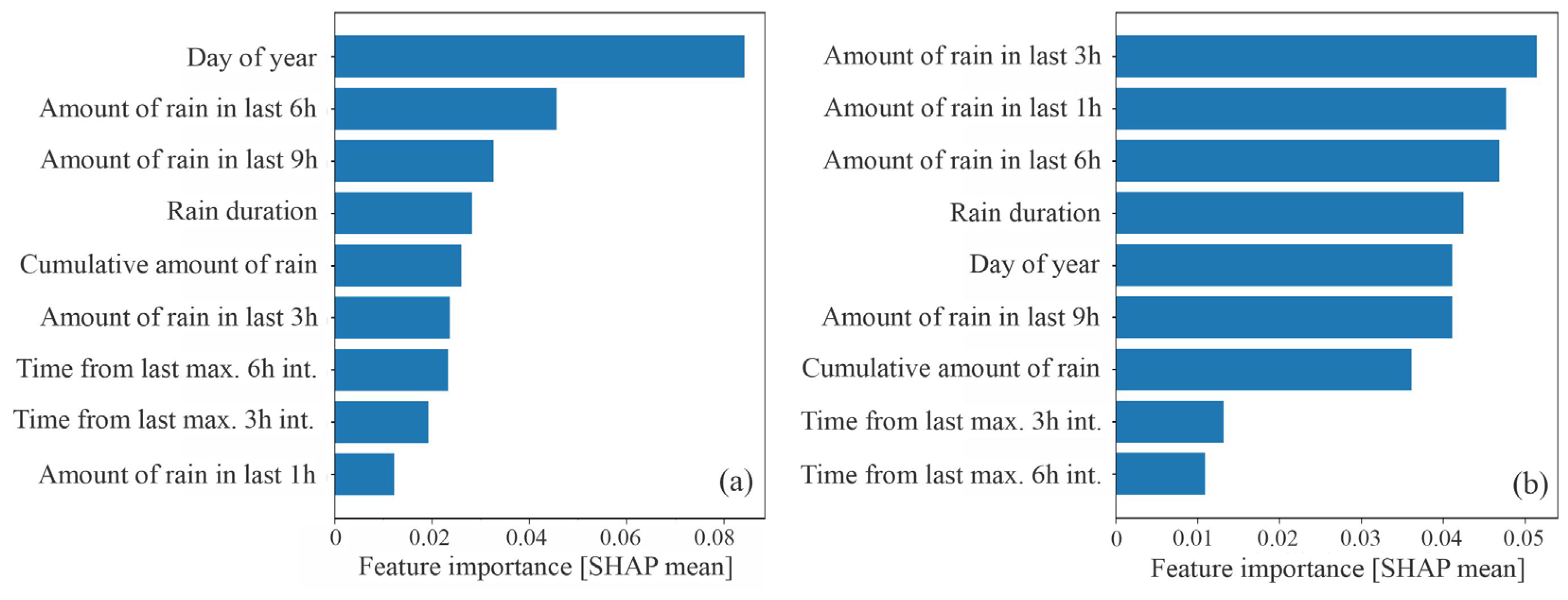
For each event, the corresponding day_of_year, rain_duration, cumulative_amount_of rain, rolling_amount_of_rain in the last 1 h, 3 h, 6 h, 9 h, the maximum_intensity in the last 3 h and 6 h, and time from last maximum 3 h and 6 h intensity were calculated. For this set of features the overall classification, accuracy, and feature importance using SHAP values from the Random Forest model were calculated. Distinctive results between SHP1 and SHP2 are shown in Figure 14.

For SHP1 (Figure 14a) the most influential features are day_of_year and amount_of_rain in last 6 h and 9 h, followed by features rain_duration and cumulative_amount_of_rain. The significantly higher signature for day of year (0.084) suggests a strong seasonality. For SHP2 (Figure 14b), the highest feature importance was achieved by amount_of_rain in the last 3 h, 1 h, 6 h and rain_duration. The day_of_year has a reduced importance of 0.041. This indicates a more direct dependence on recent rainfall accumulation rather than seasonality. The result may be explained with the distinctive technical characteristics of both SHPs. Since SHP1 uses the drop intake gate, which is more prone to leaf clogging, which mainly happens in the leaf fall period, even a small amount of rain can trigger a long event. On the other hand, events in SHP2 are triggered mainly due to the large amount of rain fall in the last 3, 1, 6, and 9 h. The SHP2 uses an automated trash rack debris removal system, which becomes clogged at higher water flow rates and the corresponding amount of debris. Therefore, only a large amount of rain may trigger the event. A detailed feature-level comparison based on the SHAP beeswarm plot is provided in Appendix B.

4.2. Decision Surface Visualization for Long Event Classification

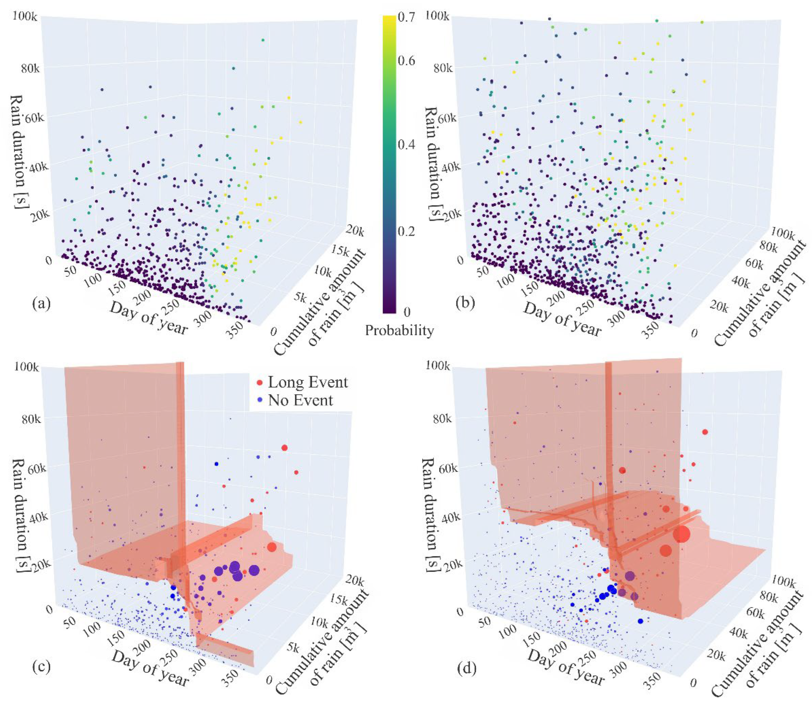
Three-dimensional (3D) surface visualization for long events gives an insight into the classification model characteristics in different operating areas. Figure 15 shows 3D surface visualization of two classification models trained to identify long events at SHP1 and SHP2. Figure 15a,b shows the probabilistic output for both classification models, while Figure 15c,d indicates the model’s decision boundary where predicted probability reaches the classification threshold. The threshold level for SHP1 is 0.32 and 0.4 for SHP2, which were defined manually focusing on achieving the best separation surface between long and no events. In this way, the model was effectively evaluated, and overfitting was avoided. However, we found that the features day_of_year, rain_duration, and cumulative_amount of_rain were the most suitable for model visualization and manual evaluation.

The decision surface of the SHP1 model extends irregularly and sparsely across the feature space, with large vertical and horizontal planes intersecting a wide range of durations and rainfall values. In autumn, the decision boundary is irregular and diffuse, indicating that the model does not clearly separate long events from no events. In contrast, the SHP2 model produces a more coherent and compact decision surface, concentrated in the region of high rainfall and longer durations.

4.3. Model Performance Comparison

To evaluate the performance of the classification models, precision, recall, F1-score, accuracy, and confusion matrices were calculated (

Table 5. Model performance metrics for SHP1 and SHP2: accuracy, precision, recall, F1-score (± variance).

	Precision	Recall	F1-Score	Support
SHP1
Class no_event	0.94	0.98	0.96	520
Class long_event	0.59 ± 0.18	0.31 ± 0.13	0.41 ± 0.14	51
Accuracy			0.92 ± 0.02	571
SHP2
Class no_event	0.96	0.93	0.95	756
Class long_event	0.55 ± 0.09	0.68 ± 0.09	0.61 ± 0.08	92
Accuracy			0.90 ± 0.02	848

, Figure 16). The results of the variance across folds are provided in Appendix B.

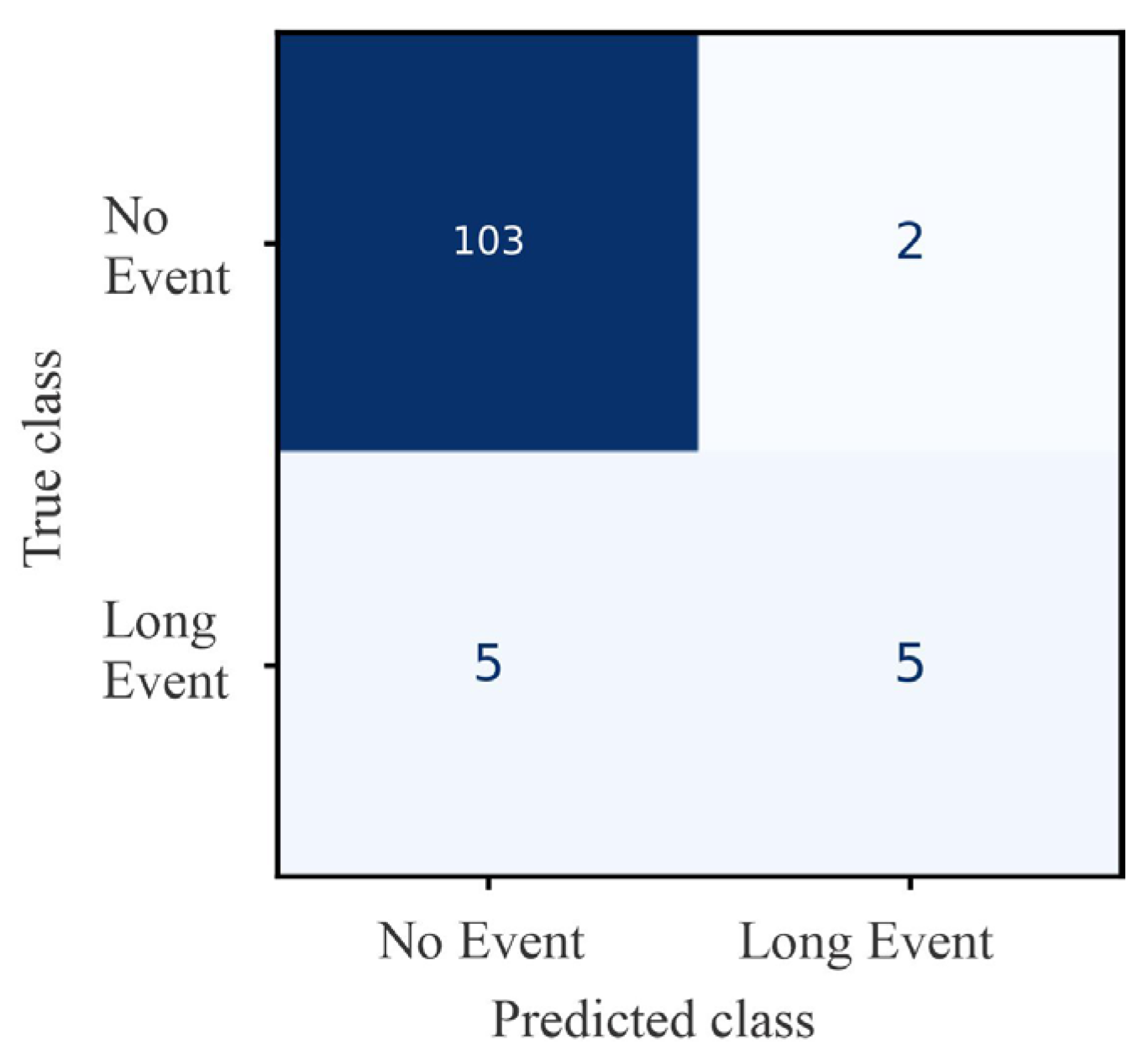
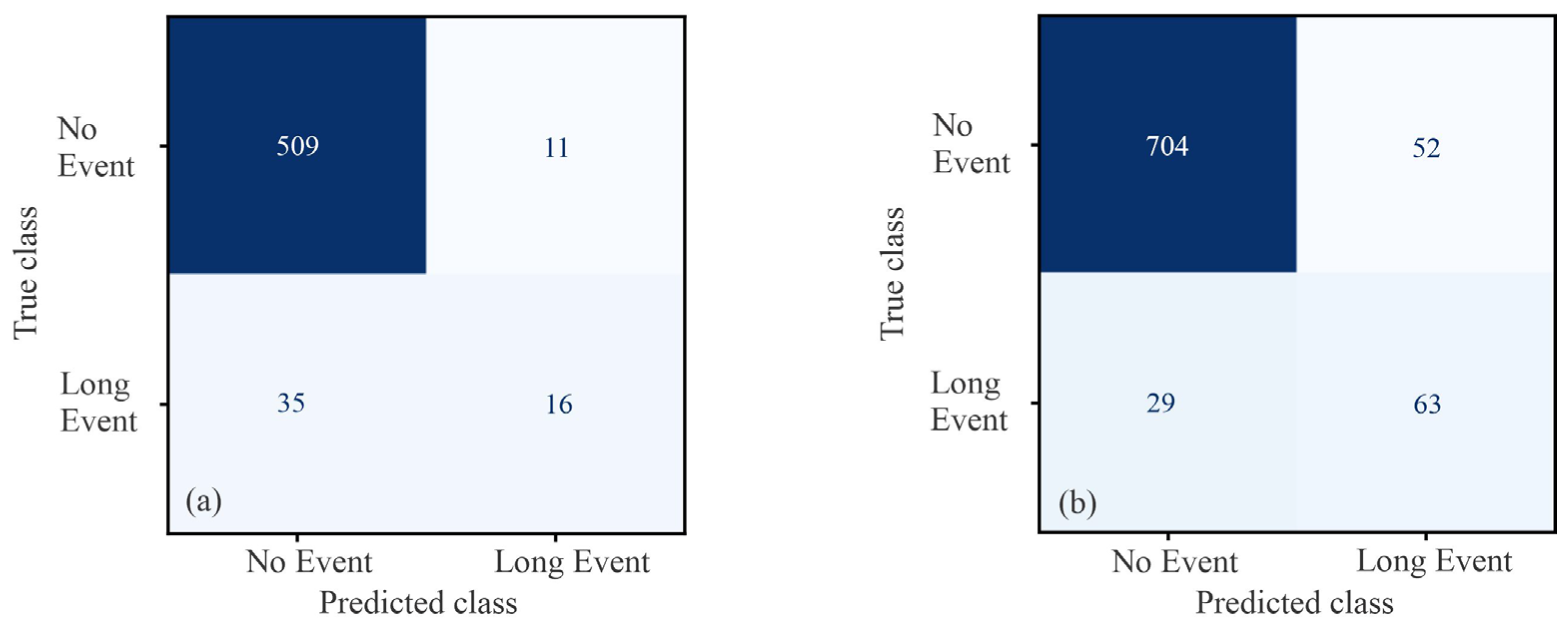
The model trained and evaluated on SHP1 data achieved an overall accuracy of 92%. Performance on the no_event class was very strong, with a precision of 0.94, recall of 0.98, and an F1-score of 0.96. For the long_event class, the model achieved a precision of 0.59, but recall was much lower at 0.31, resulting in an F1-score of 0.41. This indicates that while false alarms (no_event misclassified as long_event) were relatively rare, the model missed the majority of true long events. The confusion matrix in Figure 16a confirms this, showing that 35 out of 51 long events were misclassified as no_event.

On the SHP2 dataset, the model achieved an overall accuracy of 90%. For the no_event class, performance remained high with precision 0.96, recall 0.93, and F1-score 0.95. The long_event class performed better than in SHP1, with precision of 0.55 and recall of 0.68, resulting in an F1-score of 0.61. As shown in Figure 16b, 29 out of 92 long events were missed, but the model also detected 63 correctly, demonstrating improved sensitivity compared to SHP1.

Overall, both models exhibit strong capability in identifying no_event cases but struggle with detecting long events, which are underrepresented in the dataset. The SHP2 model outperforms SHP1 in recall and F1-score for long_event, indicating better balance between missed events and false alarms. These results also suggest that the default decision threshold favors precision in the no_event class at the expense of recall for long_event. Adjusting the threshold could increase long_event detection, though at the cost of introducing more false positives.

4.4. Finding the Optimal Feature Set and F1-Score

To identify the most effective feature subset and classification model, the machine learning algorithms described in Section 2.2 were evaluated across different combinations of input features. All possible combinations of three to six features selected from dataset 1 presented in Table 3 were generated. For each feature combination (total 42 features sets), all five models were trained and evaluated, resulting in a total of 210 feature–model combinations.

Model training and evaluation were performed using 5-fold stratified cross-validation. Out-of-fold probability estimates were obtained for each sample, ensuring that every prediction was made on data unseen during training. Based on these probabilities, a precision–recall curve was constructed, and the F1-score was calculated across all possible classification thresholds. The threshold that maximized the F1-score on the complete set of out-of-fold predictions was selected as the global decision threshold.

The top 10 classification models, sorted by F1-score along with their corresponding threshold values and features, are shown in

Table 6. Top three model configurations and model types for SHP1 and SHP2, sorted by F1-score maximization. Model visualizations are shown in Appendix C and Appendix D.

Nr.	Rank	Algorithm	F1-Score (long_event)	Threshold	Confusion Matrix	Features
						SHP1
1	1	k-NN	0.576	0.257	[[482  38] [ 15  36]]	(day_of_year, cumulative_amount_of_rain, amount_of_rain_in_last_1h, amount_of_rain_in_last_3h)
2	2	Gradient Boosting	0.566	0.193	[[478  42] [ 14  37]]	(day_of_year, cumulative_amount_of_rain, amount_of_rain_in_last_1h, amount_of_rain_in_last_3h, amount_of_rain_in_last_9h)
3	3	k-NN	0.562	0.162	[[467  53] [ 10  41]]	(day_of_year, rain_duration, amount_of_rain_in_last_1h, amount_of_rain_in_last_3h)
4	33	Random Forest	0.541	0.384	[[482  38] [ 18  33]]	(day_of_year, rain_duration, amount_of_rain_in_last_3h)
5	81	Logistic Regression	0.468	0.371	[[476  44] [ 22  29]]	(day_of_year, rain_duration, amount_of_rain_in_last_3h)
6	104	SVM	0.417	0.092	[[495  25] [ 31  20]]	(day_of_year, cumulative_amount_of_rain, amount_of_rain_in_last_1h)
						SHP2
1	1	Gradient Boosting	0.680	0.214	[[714  42] [ 23  69]]	(day_of_year, rain_duration, cumulative amount_of_rain, amount_of_rain_in_last_1h, amount_of_rain_in_last_3h, amount_of_rain_in_last_9h
2	2	Gradient Boosting	0.676	0.147	[[709  47] [ 21  71]]	(day_of_year, rain_duration, cumulative amount_of_rain, amount_of_rain_in_last_1h, amount_of_rain_in_last_3h)
3	3	Gradient Boosting	0.670	0.427	[[727  29] [ 31  61]]	(day_of_year, rain_duration, amount_of_rain_in_last_1h, amount_of_rain_in_last_9h)
4	14	SVM	0.664	0.187	[[712  44] [ 30  62]]	(day_of_year, rain_duration, amount_of_rain_in_last_3h)
5	15	k-NN	0.626	0.297	[[725  31] [ 36  56]]	(day_of_year, rain_duration, amount_of_rain_in_last_3h)
6	23	Random Forest	0.615	0.437	[[704  52] [ 28  64]]	(day_of_year, rain_duration, amount_of_rain_in_last_3h)
7	111	Logistic Regression	0.552	0.408	[[693  63] [ 33  59]]	(day_of_year, rain_duration, amount_of_rain_in_last_3h, amount_of_rain_in_last_9h)

. In the table, the top three ranked models are listed, and the first appearance of each algorithm is also indicated (e.g., the best Random Forest model in SHP1 was ranked 33rd). Visualizations of some of the most indicative models are provided in Appendix A and Appendix B.

For SHP1, the highest F1-score achieved was 0.576 (via k-NN and Gradient Boosting) using the features day_of_year, cumulative_amount_of_rain, amount_of_rain_in_last_1h, and amount_of_rain_in_last_3h. This indicates that the classifier’s ability to distinguish long_event from no_event in this dataset is moderate. For SHP2, the top F1-scores were substantially higher, ranging from 0.670 to 0.680 (Gradient Boosting). The highest-ranked classifier used the features day_of_year, rain_duration, cumulative_amount_of_rain, amount_of_rain_in_last_1h, amount_of_rain_in_last_3h, and amount_of_rain_in_last_9h. From the ranking, it is evident that a larger feature set results in a higher F1-score, while reducing the number of features leads to a weaker performance.

In SHP1, the best model correctly detected 36 long events, with 15 missed detections (false negatives) and 38 false alarms (false positives). In SHP2, the best model correctly detected 69 long events, with 23 missed detections and 42 false alarms. Both models exhibit similar trade-offs between false alarms and missed detections, but SHP2 achieves a more favorable balance between recall and precision, which is reflected in the higher F1-score.

In SHP1, a total of 51 long events were recorded, whereas in SHP2 there were 92 such events. This difference in sample size likely contributes to the higher F1-scores achieved for SHP2. The results suggest that the number of events is critical for model performance. Equally important is that the events are well distributed throughout the year and across the full range of feature values, ensuring that the model learns representative patterns of when and under which conditions long events occur. Both the quantity and the diversity of events play decisive roles in determining predictive accuracy.

For SHP1, the Random Forest (F1 = 0.541) and Gradient Boosting (F1 = 0.566) provided decision boundaries that were easier to interpret visually (Appendix C), which is important for operational insights. For SHP2, the SVM (F1 = 0.664) and Random Forest (F1 = 0.615) produced the cleanest decision surfaces (Appendix D), making them attractive alternatives despite not achieving the absolute best F1-scores. Visual model comparison also shows that in SHP1, Gradient Boosting and Random Forest align particularly well with the leaf fall period, capturing seasonal dynamics effectively.

The differences between SHP1 and SHP2 can be partly attributed to their structural and operational characteristics. SHP1, which is less automated and more sensitive to local rainfall fluctuations, benefits from the non-parametric k-NN approach, as this method effectively captures localized irregularities in the feature space. In contrast, SHP2—equipped with a rubber dam and a higher degree of operational stability—exhibits a stronger dependence on aggregate precipitation dynamics. This makes ensemble methods such as Gradient Boosting particularly effective. This is also confirmed by the SVM model which has a rank at 104. These findings highlight that the optimal machine learning model may depend on the SHP’s design and level of automation, rather than rainfall patterns alone.

Logistic Regression, which separates classes linearly, performed considerably worse than the nonlinear models. For SHP1, Logistic Regression achieved an F1-score of 0.468, compared to 0.576 for k-NN. For SHP2, Logistic Regression reached an F1-score of 0.552, while Gradient Boosting achieved 0.680. These results indicate that linear separation is insufficient for SHP2, where nonlinear interactions between rainfall features are more pronounced, whereas in SHP1 the gap between linear and nonlinear approaches is less substantial.

To assess whether the machine learning approach provides added value compared to simple rule-based methods, we also implemented a rainfall-threshold heuristic baseline. For each dataset (SHP1 and SHP2), thresholds on cumulative rainfall were scanned in the range 0–60,000 in 1000-unit increments, and the F1-score for the long_event class was computed. For SHP1, the highest F1-score achieved by the threshold-based method was 0.35 at T = 4000. For SHP2, the best threshold was T = 11,000 with an F1-score of 0.47. All nonlinear models perform substantially better. This clearly demonstrates that simple one-dimensional threshold rules are insufficient for reliably distinguishing long events, as they fail to capture the multidimensional patterns. Overall, this suggests that nonlinear models should be preferred for O&M prediction in SHPs.

To assess the robustness and transferability of the O&M models to previously unseen SHP locations, a cross-site validation was performed. The best-ranked model on SHP1 (k-NN) was trained on SHP1 and evaluated on SHP2, while the top-ranked model from SHP2 (Gradient Boosting) was trained on SHP2 and evaluated on SHP1. The cross-site evaluations showed a decline in performance compared to the within-site baselines. While site-specific models achieved F1-scores of 0.576 ± 0.118 (SHP1→SHP1) and 0.680 ± 0.076 (SHP2→SHP2), the cross-site results dropped to 0.444 ± 0.071 (SHP1→SHP2) and 0.338 ± 0.143 (SHP2→SHP1). These results confirm that O&M models are highly site-specific, highlighting the need for locally trained O&M models.

4.5. Performance of Event Classification Models on SHP1 and SHP2

The question addressed in this analysis was how much data is needed to predict events. To evaluate this, we used the F1-score and the area under the ROC curve (AUC) as performance measures. The AUC measures the model’s ability to distinguish between classes, with 0.5 indicating random guessing and 1.0 indicating perfect separation. Initially, one year of data were used for training and the following unseen year for testing. Next, two years of data were used for training and one year for testing. In the final setup, six years of data were used for training and one year for testing. Figure 17a,b show the resulting metrics for SHP1 and SHP2. The comparison was performed using a Gradient Boosting classifier trained on the features day_of_year, rain_duration, cumulative_amount_of_rain (SHP1), and an SVM classifier trained on the features day_of_year, rain_duration, amount_of_rain_in_last_3h (SHP2), which were identified as the best-performing models (see Section 3.4).

With only one year of training data, both classifiers struggled, leading to very low F1-scores despite moderate to high AUC values. As more years were added for training, the F1-score improved, demonstrating that additional historical data are essential for more reliable event prediction. For SHP1, the best results were obtained with 3–4 years of training data, whereas SHP2 achieved its best performance with 5–6 years of training data. After this time, both models were generally able to separate event from no event cases well (high AUC), but translating this into precise predictions (F1) remained challenging due to class imbalance and threshold sensitivity.

4.6. Threshold-Based Long Event Predictions and Model Probability Comparison

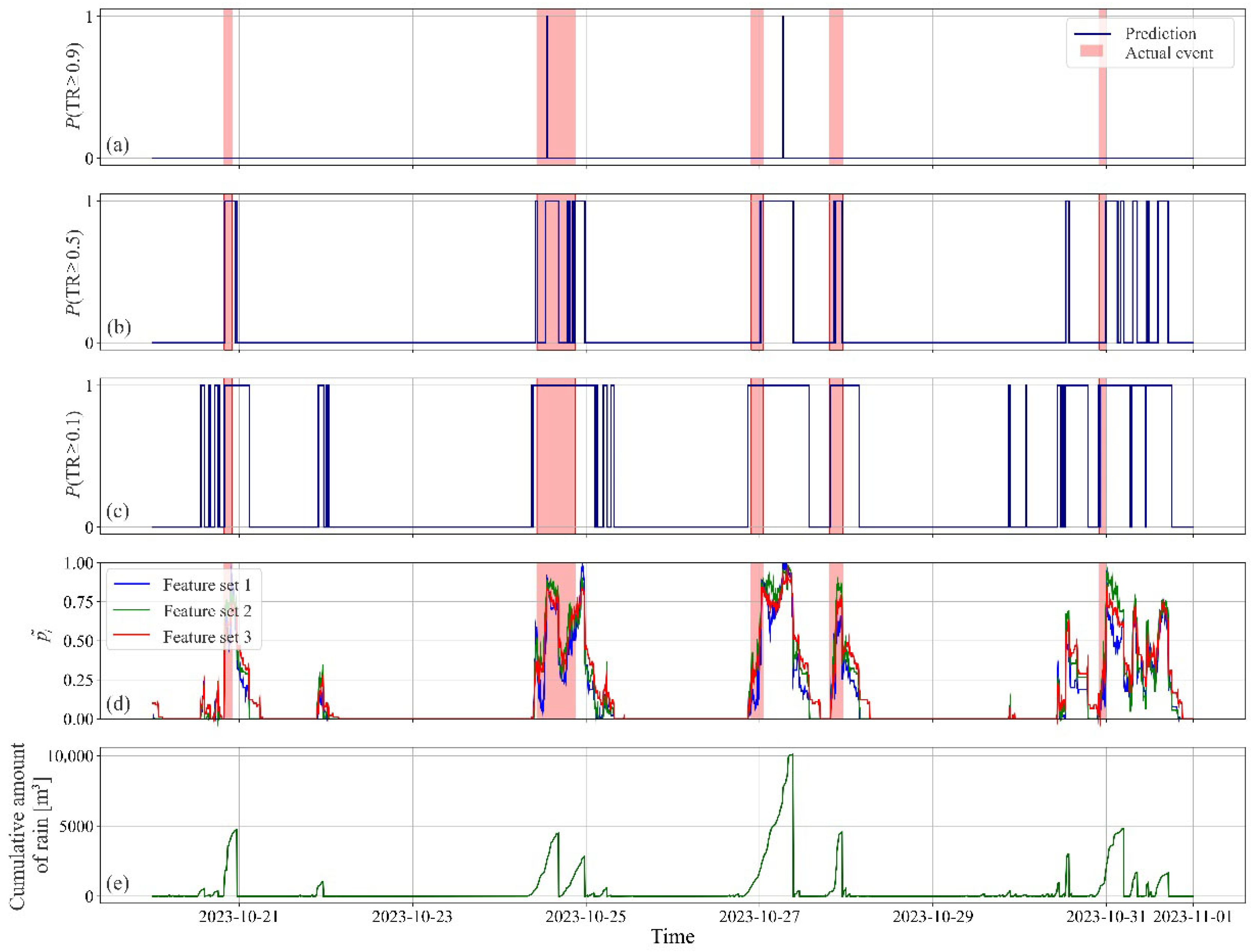
For the demonstration, the Random Forest model was used for threshold-based long event prediction. Figure 18 presents visualization of long event prediction behavior, model probability outputs, and corresponding cumulative rainfall patterns from 20 October to 1 November 2023. Subplots 18a–c show binary predictions of long events for three different probability thresholds:

-

Figure 18a (T = 0.9): High threshold leads to highly conservative predictions—long events are predicted only during periods of very high model confidence. Almost all potential events are missed.

-

Figure 18b (T = 0.5): Balanced threshold—predictions align better with the actual events (red shaded areas), but some events are still missed or fragmented.

-

Figure 18c (T = 0.1): Low threshold—very sensitive; many periods are predicted as long events, including numerous false positives.

Each blue vertical line indicates a prediction of a long event, and red shaded regions represent the true long events in time. Prediction quality is strongly dependent on threshold selection: higher thresholds reduce false positives but risk missing true events; lower thresholds increase recall but also false alarms.

The predictions from Figure 18a–c were merged with the threshold-consistency approach described in Section 3.4. For comparison, three feature sets were generated. All three feature sets include day_of_year, rain_duration, and cumulative_amount_of_rain, but differ in rolling_amount_of_rain fallen in the last 3 h (feature set 1), 6 h (feature set 2), 9 h (feature set 3). The results are presented in Figure 18d. Distinct rainfall pulses align well with predicted long event probabilities and actual event timings, especially during multi-day rainy periods. By adding features of the rolling_amount_of_rain, the models respond similarly, which confirms that adding additional features does not improve long_event prediction probability.

4.7. O&M Event Prediction Based on Radar Images and ALADIN Forecasts

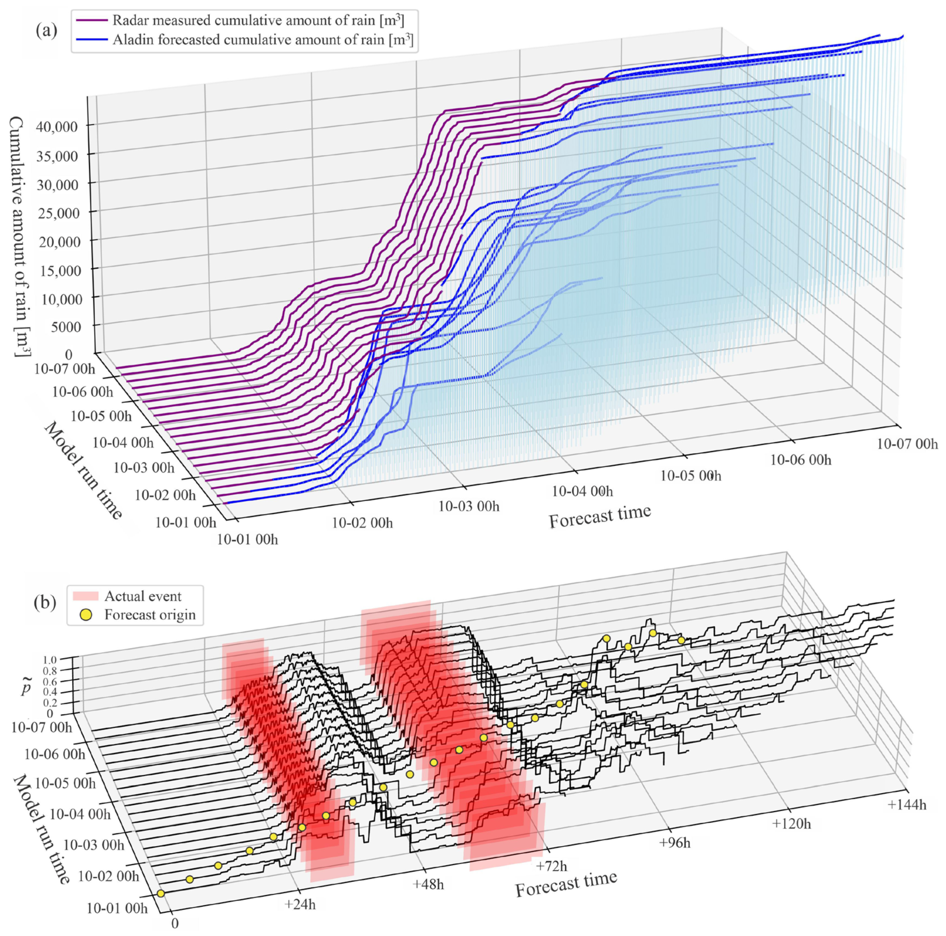
The actual model prediction model behavior during the raining period which occurred in the period of 1–7 October 2024 is shown in Figure 19a. The figure visualizes how well the ALADIN forecast matches actual rainfall. Good agreement is seen where blue and purple lines are close. Discrepancies show underprediction or overprediction by the model. The 3D stacking by run time helps evaluate temporal consistency in forecasts. During the first event, the observed cumulative rainfall was slightly lower than predicted. In the second event, the forecast initially overestimated the rainfall, followed by a short period of underestimation, and eventually returned to an overestimation toward the end of the event.

Figure 19b illustrates how the probability of long events in SHP1 evolves with respect to forecast time and model run time. Random Forest algorithm and day_of_year, rain_duration, rolling_amount_of_rain_in_last_1h, rolling_amount_of_rain_in_last_3h (feature set 1) were used for the O&M model generation. The features calculation is explained in Section 2.8. The red shaded regions represent the actual events, while the black lines show the model predicted probability. Good agreement is indicated when high values of probability occur before or during the actual events (i.e., within the red highlighted regions), demonstrating the model’s ability to anticipate long events. This plot helps visualize whether the model predicted long events before or during the actual occurrences. If black curves show high probability in or near red regions, the model performed well. If high predictions occur far from actual events, or actual events are missed entirely, the model’s performance is weaker.

There is a discrepancy between the forecasted and actual raining start times, typically ranging between 1 and 3 h (Figure 19b). Prior to the first event, a small amount of rain was recorded approximately 12 h before the actual onset, potentially contributing to early probability rises. The first event was shorter in duration than predicted. Part of this discrepancy can be attributed to the fact that event duration was not included as a feature in the training model, which may have reduced the accuracy of the duration prediction. For the second event, the predicted probability increased only after the rainfall had already occurred, indicating that the event probability was likely underestimated. However, this is due to the ALADIN uncertainty. In future work, the inherent variability of the ALADIN forecast model should also be explicitly incorporated.

5. Conclusions and Discussion

A methodology for predicting operation and maintenance (O&M) activities in run-of-river small hydropower plants (SHPs) was developed and validated to two SHPs operating on the same river. Both SHPs utilize Francis-type turbines, but their water intake systems differ—SHP1 has a Tyrolean-type weir, while SHP2 employs a rubber dam with side water withdrawal. The key findings are summarized as follows:

1.

Machine learning enables predictive O&M in SHPs. The study demonstrates that machine learning algorithms can effectively predict long O&M events in SHPs based on environmental and operational data. By training models on historical power production and precipitation data, long events, especially those triggered by rainfall, can be predicted with reasonable accuracy. This predictive ability supports proactive maintenance planning, potentially reducing operation and maintenance costs.

2.

Feature relevance differs across SHP configurations. The most important predictive features vary depending on the SHP’s design and operational context. SHP1, which uses a Tyrolean weir and is more susceptible to seasonal leaf clogging, exhibited strong dependence on the day of the year. In contrast, SHP2, equipped with a better automated trash rack system, showed stronger correlations with recent rainfall intensity. This highlights the need to tailor predictive models to each SHP’s unique characteristics.

3.

Class imbalance and threshold tuning impact model performance. While classification accuracy was high overall, recall for the long_event was lower, indicating missed events unless thresholds were carefully tuned. The models tended to favor the dominant no_event class. Threshold tuning and F1-score optimization helped improve balance, but care must be taken to avoid excessive false positives or missed events—both of which carry operational risks.

4.

Visual model interpretation is a strong tool for manual model evaluation. Visual interpretations, such as 3D decision surfaces and feature plots, offer valuable insight into model characteristics, especially in imbalanced or complex datasets where metrics like threshold tuning and F1-score optimization may be insufficient. It helps threshold tuning and reveals how features influence predictions and uncover overfitting.

5.

Radar and forecast precipitation data are viable inputs. Weather radar and ALADIN forecast data provide sufficient temporal and spatial resolution to support event prediction in mountainous SHP catchments. Despite inherent spatial limitations, especially in mountainous terrain, precipitation data interpolated over river basins provided reliable indicators for O&M event forecasting. This supports the integration of existing meteorological infrastructure for O&M event prediction, reducing the need for installing additional sensors at each SHP location.

To further improve the performance of the methodology, additional environmental variables should be incorporated. Monitoring attributes such as snow thickness, debris accumulation, freezing temperatures, and leaf fall dynamics could significantly enhance prediction accuracy. Integrating water level measurements could also provide valuable insights, particularly for detecting partial trash rack blockades that do not necessarily impact output power but require operator intervention. Additionally, refining precipitation forecasting models by comparing and integrating different weather models would further enhance the accuracy of long event prediction.

Recent advances in deep learning combined with chaos theory demonstrate substantial potential for improving time series forecasting [40], for accurate wind speed forecasting [41] and wind power fluctuation [42]. Long short-term memory (LSTM) networks show promising performance for rainfall-runoff modeling [43] and also long-term hydropower forecasting [44]. Incorporating new approaches for predicting nonlinear and dynamic relationships could further improve event prediction, particularly during complex seasonal conditions and periods of high water flow.

One of the strengths of this methodology is its scalability and plant-specific adaptability. Given that radar coverage includes more than four hundred SHPs in Slovenia, the methodology enables the generation of individualized O&M models that reflect the distinct technical configurations and environmental conditions of each SHP site.

The developed methodology thus provides a valuable tool for improving the prediction of O&M activities in SHPs, leading to greater operational efficiency, cost reduction, and reliability. Ultimately, this approach has the potential to optimize O&M scheduling and increase SHP availability, benefiting both existing operators and O&M service providers.