Does Score Bias Correction Improve the Fusion of Classifiers?

Abstract

We demonstrate that the potential bias in the scores generated by individual classifiers negatively affects their fusion. Consequently, we present an algorithm to improve the effectiveness of score fusion in classification. The algorithm corrects the score class conditional bias before fusion. The interest of the procedure is demonstrated theoretically, first in general terms and then considering exponential models for the score class conditional distributions. The case of beta distributions is also addressed using Monte Carlo simulations. Finally, a real-life application of fusion of two modalities (EEG, ECG) and two classifiers (Gaussian Bayes and Logistic Regression) is included, showing significant improvement with respect to conventional fusion without bias correction.

1. Introduction

Fusion of scores is of interest whenever different entities collaborate to arrive at a common opinion on the occurrence of a given phenomenon. This is particularly relevant in the fusion of automatic classifiers where a score is to be assigned to each possible class [1,2,3,4,5,6,7]. Fused classifiers can correspond to one or several modalities. In the latter case, the term “multimodal fusion” is often used [8,9,10,11,12,13,14,15]. In the Bayesian approach, the scores can be considered posterior probabilities of each class, so they are restricted within the range 0–1 and must add up to 1. This imposes a relevant limitation on the score fusion framework, as explained below.

Let us consider the two-class problem $c=\mathrm{0,1}$. Given a feature vector $\mathit{x}$, a score $s$ within (0, 1) is assigned to class $c=1$, and a score $1 - s$ is assigned to class $c=0$. Therefore $s$ can be considered an estimate of a binary random variable from a given feature vector $\mathit{x}$. A good estimator should provide scores close to 1 for feature vectors belonging to class $c=1$ and close to 0 for feature vectors belonging to class $c=0$. From that perspective, notice that $s$ is inevitably a conditionally biased estimate. This is immediately evident. Let us call $p\left(s/c=i\right)$ to the probability density function (PDF) of $s$ conditional to class $c=i$. Moreover, conditional to class $c=i$, the true value of the binary random variable will be $i$. Then, let us compute the conditional biases $b_0$ and $b_1$ (for simplicity in the rest of the analysis, we define the bias so that both are positive).

$$\begin{gathered} b_0=E\left(s/c=0\right)-0=\underset{\ge 0}{\underbrace{{\int }_0^{1}s\cdot p\left(s/c=0\right)ds}}-0\Rightarrow 0\le b_0\le 1 \\ {b}_1=1-E\left(s/c=1\right)=1-\underset{\le 1}{\underbrace{{\int }_0^{1}s\cdot p\left(s/c=1\right)ds}}\ge 0\Rightarrow 0\le b_1\le 1, \end{gathered}$$

(1)

where the lower bounds only hold for perfect (unrealistic) estimators, i.e., $p\left(s/c=i\right)=\delta \left(s-i\right)$. These (inevitable) biases impose a limitation on classifier performance. Let us demonstrate it from a rather inverse perspective: if we could compensate the bias, the detector performance would improve. Before that, let us assume that we use a maximum a posteriori (MAP) criterion, where the most probable class is selected, i.e., as follows:

$$s\begin{array}{c}\stackrel{c=1}{>}\\ \underset{c=0}{<}\end{array}1-s\iff s\begin{array}{c}\stackrel{c=1}{>}\\ \underset{c=0}{<}\end{array}0.5 .$$

(2)

This implicitly assumes that the scores are calibrated, that is, that P(c = 1/s) = s. However, there is no conceptual problem in implementing the bias correction method described in the following section with uncalibrated scores. In fact, the goal of the correction method is to improve accuracy (a “post-thresholding indicator”), whereas calibration refers to using the scores as probabilities of class membership (a “pre-thresholding indicator”). Therefore, calibration and correction can be complementary; for example, it will always be possible to calibrate the corrected scores.

Equation (2) defines the two-class classification problem as a detection problem, where class $c=1$ is detected when the statistic $s$ is greater than the threshold 0.5 (the term detector will be frequently used throughout the article). As we see bellow, if we could correct the conditional bias $b_0$, the probability of false alarm $PFA={\int }_{0.5}^{1}p\left(s/c=0\right)ds$ will decrease and if we could correct the conditional bias $b_1$, the probability of detection $PD={\int }_{0.5}^{1}p\left(s/c=1\right)ds$ will increase. Correcting $b_0$ involves a shift to the left (towards 0) of $p\left(s/c=0\right)$, while correcting $b_1$ involves a shift to the right (towards 1) of $p\left(s/c=1\right)$. Let us call $PF{A}_b$ and $P{D}_b$ to the corresponding probabilities after bias correction, then

$$\begin{gathered} PF{A}_b={\int }_{0.5}^{1-b_0}p\left(s+b_0/c=0\right)ds\underset{s^{\prime }=s+b_0}{\underbrace{=}}{\int }_{0.5+b_0}^{1}p\left(s^{\prime }/c=0\right)d{s}^{\prime }<{\int }_{0.5}^{1}p\left(s^{\prime }/c=0\right)d{s}^{\prime }=PFA \\ P{D}_b={\int }_{0.5}^{1+b_1}p\left(s-b_1/c=1\right)ds\underset{s^{\prime }=s-b_1}{\underbrace{=}}{\int }_{0.5-b_1}^{1}p\left(s^{\prime }/c=1\right)d{s}^{\prime }>{\int }_{0.5}^{1}p\left(s^{\prime }/c=1\right)d{s}^{\prime }=PD. \end{gathered}$$

(3)

Therefore, correcting the bias reduces $PFA$ and increases $PD$, thus improving the detector performance. Unfortunately, direct correction of the conditional bias is an ill-posed problem. Certainly, we can compute sample estimates ${\widehat{b}}_0$ and ${\widehat{b}}_1$ from labeled training data. However, compensating for the bias of the sample under test requires knowledge of the true class because we have to subtract ${\widehat{b}}_0$ from the computed score if the true class is $c=0$, but we must add ${\widehat{b}}_1$ if the true class is $c=1$. But determining the true class of the sample under test is exactly the problem we are trying to solve from the very beginning. Furthermore, averaging individual scores from different detectors to obtain a score with reduced conditional bias is not an option because the individual biases are all positive. For example, it is well-known that by averaging $N$ independent and identically distributed random variables (i.i.d.r.v.), we obtain a random variable where variance has been reduced by a factor $N$. However, the mean (and so the possible bias in an estimation context) remains the same. A more formal analysis of the conditional bias influence on the optimum fusion of classifiers is given in [16] for some specific models.

Despite the above discouraging arguments, we propose in the following section an algorithm for conditional bias correction in the framework of score fusion. We first provide an intuitive (rather heuristic) rationale of the proposal. Then, a general formal analysis is carried out. This later indicates that the expected improvement depends on the integration of the bivariate class conditional PDFs in a given area. So, in Section 3, the analytically tractable case of exponential PDFs is analyzed. Then in Section 4, we consider the more general case of beta-PDFs. Beta-distribution is the more common model for random variables in (0, 1). Unfortunately, this is analytically infeasible, so we resorted to Monte Carlo simulations. Finally, in Section 5, we evaluated the usefulness of the proposed algorithm in a real-world experiment, combining two biosignal modalities, electroencephalograms (EEGs) and electrocardiograms (ECGs), and two lightweight classifiers, Gaussian Bayes (GB) and Logistic Regression (LR), to improve sleep arousal detection.

2. The Algorithm for Conditional Bias Correction

Let us consider two individual classifiers defined, respectively, by the variable $m=\mathrm{1,2}$. Given a sample under test ${\mathit{x}}_m$, each classifier provides a score $0\le s_m\le 1$, which, according to the previous section, represents the posterior probability of class $c=1$, i.e., $P\left(c=1/{\mathit{x}}_m\right)=s_m$, and hence $P\left(c=0/{\mathit{x}}_m\right)=1-s_m$. Every classifier implements the MAP test (2) with $s_m$; hence, the corresponding probabilities of false alarm and detection will be given by

$$\begin{gathered} PF{A}_m=\mathit{Pr}\left(s_m>0.5/c=0\right)={\int }_{0.5}^1\left(s_m/c=0\right)d{s}_m \\ P{D}_m=\mathit{Pr}\left(s_m>0.5/c=1\right)={\int }_{0.5}^1\left(s_m/c=1\right)d{s}_m . \end{gathered}$$

(4)

We will assume that $s_1$ and $s_2$ are i.i.d.r.v. to facilitate the analysis, so that we can write

$$\begin{gathered} \left(s_1{s}_2/c=i\right)=p\left(s_1/c=i\right)\cdot p\left(s_2/c=i\right)=p_i\left(s_1\right)p_i\left(s_2\right) \\ PF{A}_1=PF{A}_2=PFA \\ P{D}_1=P{D}_2=PD . \end{gathered}$$

(5)

Let us start by the case of no bias correction. Scores are fused by computing the mean ${\displaystyle \frac{1}{2}}\left(s_1+s_2\right)$, which is to be compared with the 0.5 threshold as in (2). For convenience, we prefer to consider the score $=s_1+s_2$ $0\le z\le 2$, and compare $z$ with a threshold 1, which is an equivalent test. It is evident that if both original scores exceed the threshold of 0.5, their sum will exceed the threshold of 1. And vice versa if both individual scores are below the threshold of 0.5. Therefore, the possible improvement through fusion will occur when both classifiers make different decisions, such that the score of the one who makes a mistake is offset by the score of the one who makes a correct decision.

Now consider that before adding the scores we apply a conditional bias correction. Let us define the biases of every classifier as in (1): $b_{m0}=E\left[s_m/c=0\right]-0>0 b_{m1}=1-E\left[s_m/c=1\right]>0$. From assumption (5), we may simplify to $b_{10}=b_{20}=b_0$ and $b_{11}=b_{21}=b_1$. These values can be estimated during training from labeled samples, but for simplicity, we keep the notation $b_0$ and $b_1$ for the computed estimates. 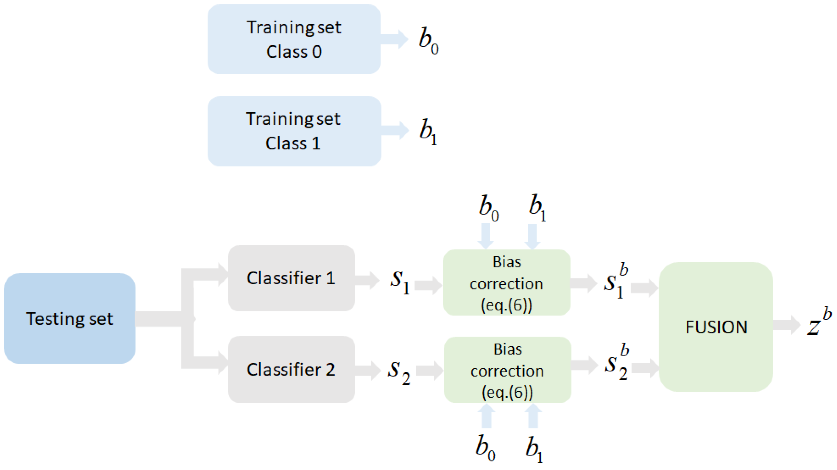The bias correction is implemented as indicated by the following equations (Figure 1 depicts the general scheme):

$$s_m^b=\left\{\begin{array}{c}{s}_m-b_0 if s_m<0.5 \\ s_m+b_1 if s_m>0.5\end{array}\right. .$$

(6)

This can be interpreted as accepting the class selected by the individual classifier as “true” to perform the corresponding correction of the conditional bias. Certainly, the individual classifier will provide both correct and incorrect decisions, depending on its own performance (essentially its operating point given by $P{D}_m$ and $P{FA}_m$). The following analysis deduces the expected performance of the proposed method, implicitly incorporating the performances of the individual detectors.

First notice that working with the corrected scores by no means modifies the performance of the individual classifiers. This is because the bias is always positive, hence if ${ s}_m<0.5\Rightarrow s_m^b=s_m-b_0<0.5$ and if $s_m>0.5\Rightarrow s_m^b=s_m+b_1>0.5$. Consider now that the fusion consists of $z^b=s_1^b+s_2^b$ $-2b_0\le z^b\le 2+2b_1$, and compare $z^b$ with a threshold of 1. Again, if both original scores exceed the threshold of 0.5, then $z^b=s_1+s_2+2b_1>1$. But if both original scores are below the threshold of 0.5, then $z^b=s_1+s_2-2b_0<1$. Therefore, as with $z$, the potential improvement using $z^b$ will be obtained in cases where individual classifiers make different decisions, i.e., the following:

$$z^b=s_1+s_2+b_1-b_0\left\{\begin{array}{c}where s_1>0.5{ s}_2<0.5\\ where{ s}_1<0.5 s_2>0.5 \end{array}.\right.$$

(7)

Obviously, if $b_1=b_0\Rightarrow z^b=z$, i.e., the correction of biases does not contribute anything with respect to conventional fusion. However, let us assume that the class to be detected, as defined in (2), is the one with the most biased scores, i.e., $b_1>b_0\Rightarrow z^b>z$. Therefore, if the correct decision in (7) is $c=1$, bias correction will contribute to increasing the probability of detection. Certainly, if the correct decision is $c=0$, bias correction will contribute to increasing the probability of false alarm. But, considering that $b_1>b_0$ (the scores corresponding to $c=1$ are “worst” than the scores corresponding to $c=0$), disagreement events of the type (7), should be more likely when the true class is $c=1$. Then, it is expected that the increasing probability of detection will be more “significant” than the increasing probability of false alarm. This rather heuristic argument encourages us to undertake a formal analysis of the procedure, as we do below.

Let us call, respectively, $P{D}_z$ and $PF{A}_z$ the probability of detection and false alarm of $z=s_1+s_2$, and $P{D}_{z^b}$ and $PF{A}_{z^b}$ the probability of detection and false alarm of $z^b=s_1^b+s_2^b$. Our aim is to deduce how $P{D}_z$ and $PF{A}_z$ change when bias correction is implemented, i.e., to deduce the relation between $P{D}_{z^b}$ and $P{D}_z$, as well as $PF{A}_{z^b}$ and $PF{A}_z$. But, as already stated above $z^b>z$, which allows us to ensure that $P{D}_{z^b}>P{D}_z$ and $PF{A}_{z^b}>PF{A}_z$. The increase in both probabilities will occur due to those cases in which both detectors make a different decision, being $z<1$ and $z^b>1$. Let us express this conclusion in terms of $s_1$ and $s_2$ (we define $\Delta =b_1-b_0\Rightarrow 0\le \Delta \le 1$).

$$\begin{gathered} P{D}_{z^b}=P{D}_z+2P{D}_{z^b}=P{D}_z+2\mathit{Pr}\left(s_1+s_2+\Delta >1/s_1+s_2<1,s_1<0.5,s_2>0.5,c=1\right) \\ PF{A}_{z^b}=PF{A}_z+2P{FA}_{z^b}==PF{A}_z+2\mathit{Pr}\left(s_1+s_2+\Delta >1/s_1+s_2<1,s_1<0.5,s_2>0.5,c=0\right) \end{gathered}$$

(8)

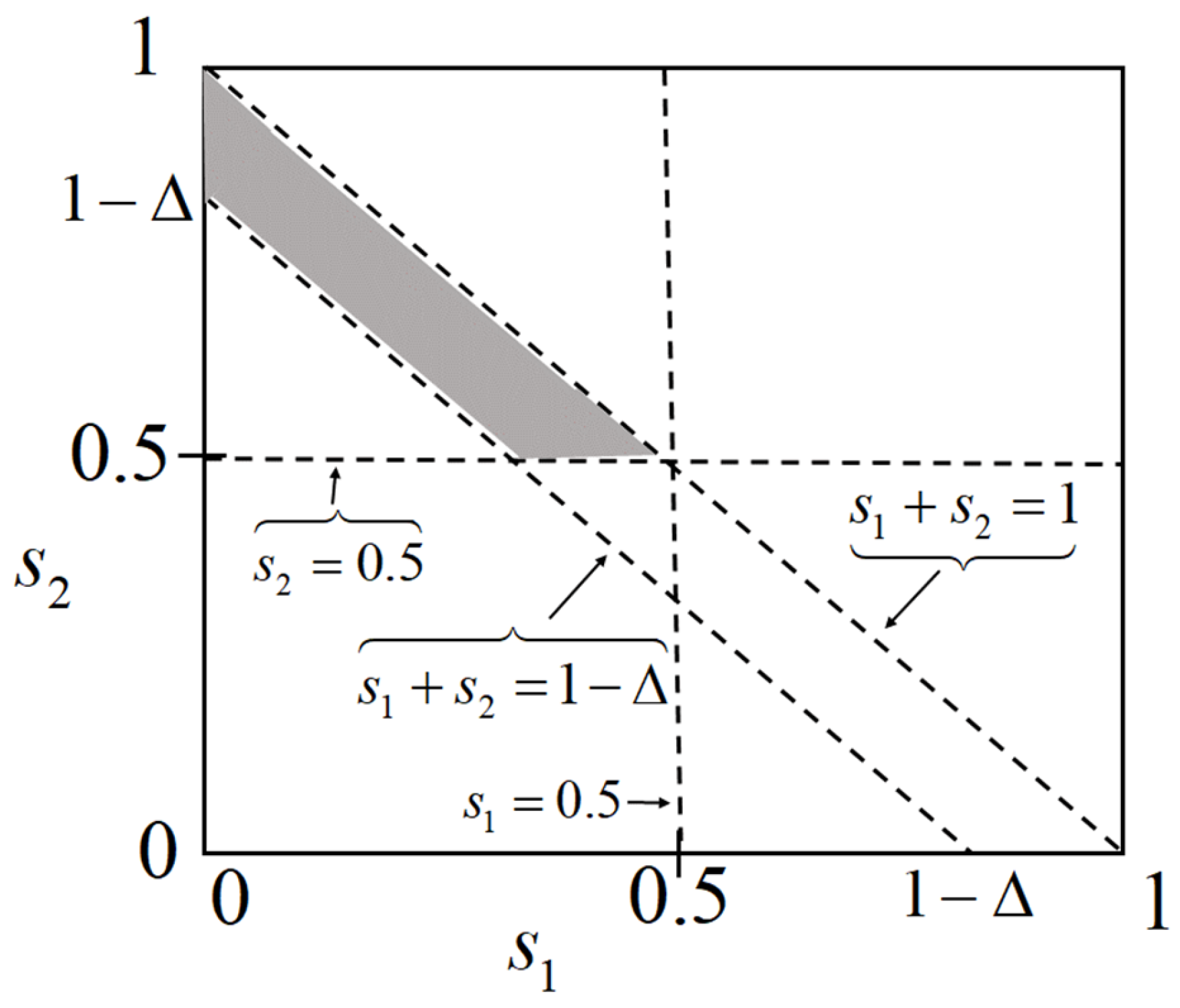
The factor 2 appears because the two events, $s_1<0.5,s_2>0.5,$ and $s_1>0.5,s_2<0.5,$ are equivalent as far as we have assumed in (5) that $s_1$ and $s_2$ have the same class conditional PDFs. Figure 2 helps us to compute the required probabilities in (8). The shadowed area corresponds to the values $s_1$ and $s_2$ that satisfy the conditioning in (8); therefore, we have to integrate the corresponding bivariate PDF in that area. From (5) and Figure 2, we can write

$$\begin{array}{c}{D}_{z^b}=P{D}_z+2\left({\int }_0^{0.5-\Delta }{\int }_{1-s_1-\Delta }^{1-s_1}{p}_1\left(s_1\right)p_1\left(s_2\right)d{s}_{1}d{s}_2+{\int }_{0.5-\Delta }^{0.5}{\int }_{0.5}^{1-s_1}{p}_1\left(s_1\right)p_1\left(s_2\right)d{s}_{1}d{s}_2\right) 0\le \Delta \le 0.5\hfill \\ P{D}_{z^b}=P{D}_z+2{\int }_0^{0.5}{\int }_{0.5}^{1-s_1}{p}_1\left(s_1\right)p_1\left(s_2\right)d{s}_{1}d{s}_2 0.5\le \Delta \le 1\hfill \\ PF{A}_{z^b}=PF{A}_z+2\left({\int }_0^{0.5-\Delta }{\int }_{1-s_1-\Delta }^{1-s_1}{p}_0\left(s_1\right)p_0\left(s_2\right)d{s}_{1}d{s}_2+{\int }_{0.5-\Delta }^{0.5}{\int }_{0.5}^{1-s_1}{p}_0\left(s_1\right)p_0\left(s_2\right)d{s}_{1}d{s}_2\right) 0\le \Delta \le 0.5\hfill \\ PF{A}_{z^b}=PF{A}_z+2{\int }_0^{0.5}{\int }_{0.5}^{1-s_1}{p}_0\left(s_1\right)p_0\left(s_2\right)d{s}_{1}d{s}_2 0.5\le \Delta \le 1.\hfill \end{array}$$

(9)

Thus, the potential improvement of fusion with bias correction depends on how the individual PDFs integrate inside the shadowed area of Figure 2. In principle, it is expected that the bivariate PDF for class $c=0$ would be concentrated in the lower left corner of the square in Figure 2, while the corresponding for class $c=1$ should be concentrated in the upper right corner. On the other hand, the greater the bias, the greater the occupancy of the bivariate PDF along the square, so the integral of $p_1\left(s_1\right)p_1\left(s_2\right)$ in the shadowed area should be larger than that of $p_0\left(s_1\right)p_0\left(s_2\right)$. A more specific conclusion requires knowledge of $p_1\left(\cdot \right)$ and $p_0\left(\cdot \right)$. Therefore, in the next section, we will consider conditional PDFs to be truncated exponentials. While this is reasonably realistic, the exponential assumption makes the analysis tractable.

Furthermore, in Section 4, we will assume the beta distribution. This is the most common distribution for random variables in the finite domain (0, 1). It covers a wide variety of distributions by adjusting two parameters. Unfortunately, a theoretical analysis for the beta distribution is not feasible, so we resort to Monte Carlo simulations.

3. The Exponential Distribution Case

Let us consider that $p_0\left(s_m\right)$ and $p_1\left(s_m\right)$ are, respectively, a truncated exponential and a transformed truncated exponential PDF in the interval (0, 1), namely the following:

$$\begin{gathered} p_0\left(s_m\right)=\left\{\begin{array}{c}{\displaystyle \frac{{\lambda }_0}{1-e^{-{\lambda }_0}}}{e}^{-{\lambda }_0{s}_m} 0\le s_m\le 1\\ 0 rest\end{array}\right. \\ {p}_1\left(s_m\right)=\left\{\begin{array}{c}{\displaystyle \frac{{\lambda }_1}{1-e^{-{\lambda }_1}}}{e}^{-{\lambda }_1\left(1-s_m\right)} 0\le s_m\le 1\\ 0 rest\end{array}\right. . \end{gathered}$$

(10)

These two exponential models, respectively, concentrate more probability as we approach $s_m=0$ from the right side or as we approach $s_m=1$ from the left side, which seems an expected property of reasonable classifiers. Moreover, according to (1)

$$\begin{gathered} b_0=E\left(s_m/c=0\right)={\displaystyle \frac{1-e^{-{\lambda }_0}}{{\lambda }_0}} \\ {b}_1=1-E\left(s_m/c=1\right)={\displaystyle \frac{1-e^{-{\lambda }_1}}{{\lambda }_1}} . \end{gathered}$$

(11)

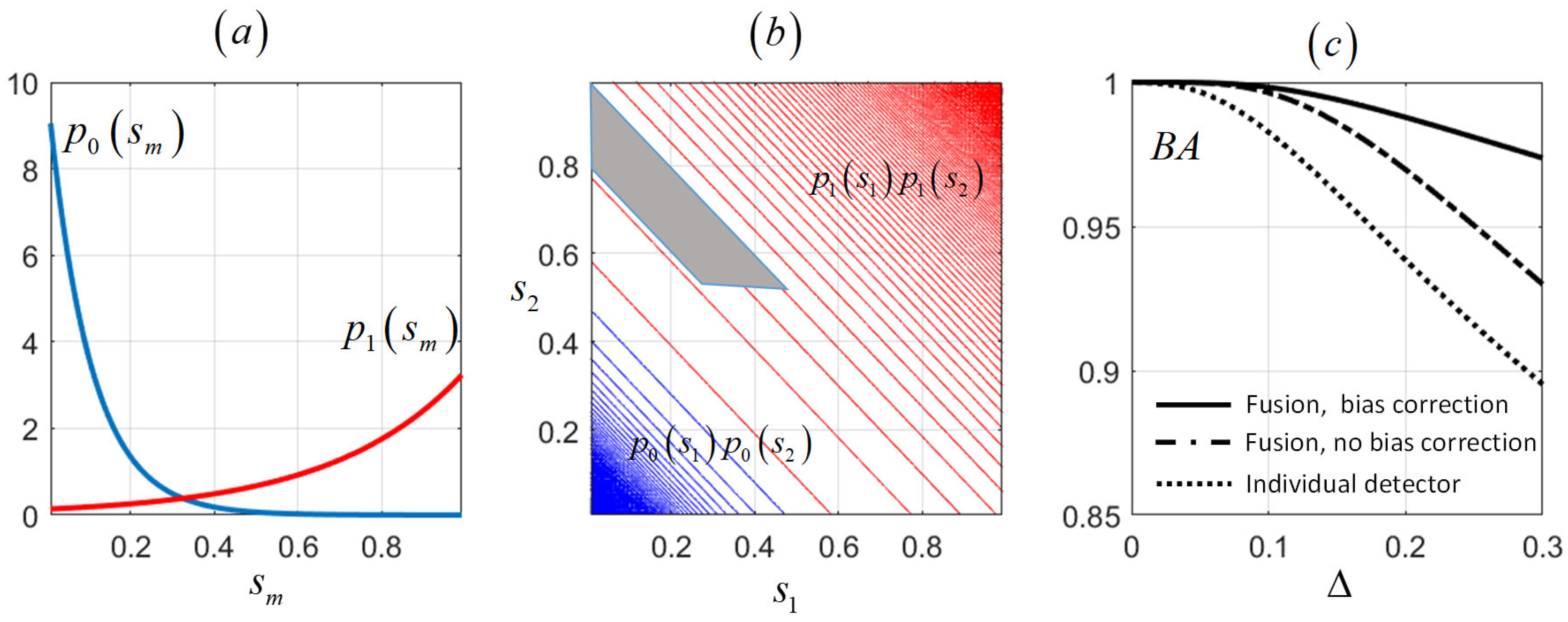
We have represented in Figure 3a two exponential distributions, where the blue one corresponds to a truncated exponential $p_0\left(s_m\right)$ with ${\lambda }_0=10\to b_0=0.1$ and the red one corresponds to a transformed truncated exponential $p_1\left(s_m\right)$ with ${\lambda }_1=3.2\to b_1=0.3$. Note that the greater the bias, the slower the decay of the exponentials. Then in Figure 3b, we have represented the contour plots of $p_0\left(s_1\right)p_0\left(s_2\right)$ (blue) and $p_1\left(s_1\right)p_1\left(s_2\right)$ (red) considering the conditional PDFs of Figure 3a. We have also marked in Figure 3b the shadowed area from Figure 2 where both bivariate PDFs have to be integrated to calculate the increase in $P{D}_z$ and $PF{A}_z$ due to bias correction. Clearly, the distribution corresponding to the class with more bias expands more along the square, leading to a greater overlap with the shaded area. Therefore, greater increase in detection probability than in false alarm probability is to be expected. In order to obtain a more precise and quantitative assessment, we have calculated the integrals in the shaded area for this exponential case. Thus, we first calculate in Appendix A the probabilities corresponding to the individual detectors and to the fusion without bias correction. The expressions obtained are

$$\begin{gathered} PD={\displaystyle \frac{1-e^{-{\lambda }_{1}0.5}}{1-e^{-{\lambda }_1}}};PFA=e^{-{\lambda }_{0}0.5}{\displaystyle \frac{1-e^{-{\lambda }_{0}0.5}}{1-e^{-{\lambda }_0}}} \\ P{D}_z={\displaystyle \frac{\left(1-e^{-{\lambda }_1}\left(1+{\lambda }_1\right)\right)}{{\left(1-e^{-{\lambda }_1}\right)}^2}};PF{A}_z={\displaystyle \frac{e^{-{\lambda }_0}\left(1-e^{-{\lambda }_0}-{\lambda }_0\right)}{{\left(1-e^{-{\lambda }_0}\right)}^2}}. \end{gathered}$$

(12)

Then, we also calculate in Appendix A the integrals required in (9) for the computation of $P{D}_{z^b}$ and $PF{A}_{z^b}$.

$$\begin{array}{c}P{D}_{z^b}=P{D}_z+2\left({\displaystyle \frac{{\lambda }_1{e}^{-{\lambda }_1}}{{\left(1-e^{-{\lambda }_1}\right)}^2}}\left(1-e^{-{\lambda }_1\Delta }\right)\left(0.5-\Delta \right)+{\displaystyle \frac{{\lambda }_1{e}^{-{\lambda }_1}}{{\left(1-e^{-{\lambda }_1}\right)}^2}}\left(\Delta -{\displaystyle \frac{1}{{\lambda }_1}}\left(1-e^{-{\lambda }_1\Delta }\right)\right)\right) 0\le \Delta \le 0.5\hfill \\ P{D}_{z^b}=P{D}_z+2\left({\displaystyle \frac{{\lambda }_1{e}^{-{\lambda }_1}}{{\left(1-e^{-{\lambda }_1}\right)}^2}}\left(0.5-{\displaystyle \frac{1}{{\lambda }_1}}\left(1-e^{-{\lambda }_{1}0.5}\right)\right)\right) 0.5\le \Delta \le 1\hfill \\ PF{A}_{z^b}=PF{A}_z+2\left({\displaystyle \frac{{\lambda }_0{e}^{-{\lambda }_0}}{{\left(1-e^{-{\lambda }_0}\right)}^2}}\left(e^{{\lambda }_0\Delta }-1\right)\left(0.5-\Delta \right)+{\displaystyle \frac{{\lambda }_0{e}^{-{\lambda }_0}}{{\left(1-e^{-{\lambda }_0}\right)}^2}}\left({\displaystyle \frac{1}{{\lambda }_0}}\left(e^{{\lambda }_0\Delta }-1\right)-\Delta \right)\right) 0\le \Delta \le 0.5\hfill \\ PF{A}_{z^b}=PF{A}_z+2\left({\displaystyle \frac{{\lambda }_0{e}^{-{\lambda }_0}}{{\left(1-e^{-{\lambda }_0}\right)}^2}}\left({\displaystyle \frac{1}{{\lambda }_0}}\left(e^{{\lambda }_{0}0.5}-1\right)-0.5\right)\right) 0.5\le \Delta \le 1 .\hfill \end{array}$$

(13)

Using the previous expressions, we can calculate the balanced accuracy $\left(BA\right)$, defined as the mean of the “sensitivity” (equivalent to probability of detection) and the “specificity” (equivalent to 1 minus the probability of false alarm), namely the following:

$$\begin{gathered} BA={\displaystyle \frac{1}{2}}\left(PD+1-PFA\right)=1-\left({\displaystyle \frac{1}{2}}\left(1-PD\right)+{\displaystyle \frac{1}{2}}PFA\right)=1-PE \\ B{A}_z={\displaystyle \frac{1}{2}}\left(P{D}_z+1-PF{A}_z\right)=1-\left({\displaystyle \frac{1}{2}}\left(1-P{D}_z\right)+{\displaystyle \frac{1}{2}}PF{A}_z\right)=1-P{E}_z \\ B{A}_{z^b}={\displaystyle \frac{1}{2}}\left(P{D}_{z^b}+1-PF{A}_{z^b}\right)=1-\left({\displaystyle \frac{1}{2}}\left(1-P{D}_{z^b}\right)+{\displaystyle \frac{1}{2}}PF{A}_{z^b}\right)=1-P{E}_{z^b}, \end{gathered}$$

(14)

where $PE, P{E}_z$, and $P{E}_{z^b}$ are the probabilities of error assuming equal priors $P_0=P_1={\displaystyle \frac{1}{2}}$. Then, we show in Figure 3c the balanced accuracies for $b_0=0.05$ and $0.05\le b_1\le 0.35\iff 0\le \Delta \le 0.30$. As expected, the balanced accuracy decreases with increasing $\Delta$, but is always higher when bias correction is applied. In fact, the improvement achieved compared to individual classifiers, as well as conventional fusion, is greater the larger $\Delta$ is.

4. The Beta Distribution Case

In the previous section, we carried out a theoretical study, made possible by the analytical tractability of the exponential distribution. However, the most common distribution for random variables in the finite domain (0, 1) is the beta distribution. This distribution is defined by two parameters, $\alpha >0$ and $\beta >0$, which allow for a wide variety of PDFs to be considered. Unfortunately, its analytical expression prevents a theoretical study like the previous one, so we will resort to Monte Carlo simulations to evaluate the effectiveness of the bias correction. Let us consider that $p_0\left(s_m\right)$ is a beta-PDF: $p_0\left(s_m\right)={\displaystyle \frac{s_m^{{\alpha }_0-1}{\left(1-s_m\right)}^{{\beta }_0-1}}{{\rm B}\left({\alpha }_0,{\beta }_0\right)}}$ where ${\rm B}\left({\alpha }_0,{\beta }_0\right)$ is the beta-function, and that $p_1\left(s_m\right)={\displaystyle \frac{{\left(1-s_m\right)}^{{\alpha }_1-1}{s}_m^{{\beta }_1-1}}{{\rm B}\left({\alpha }_1,{\beta }_1\right)}}$, which also corresponds to a beta-PDF but with interchanged parameters. Among the wide variety of beta-PDFs, we have selected some that seem appropriate for the case at hand. This was carried out by first setting a value ${\alpha }_0={\alpha }_1=\alpha$ in $p_0\left(s_m\right)$ and $p_1\left(s_m\right)$, and then calculating the values ${\beta }_0$ and ${\beta }_1$ which, respectively, give biases $b_0$ and $b_1$. Notice that ${\beta }_i={\alpha }_i{\displaystyle \frac{1-b_i}{b_i}}$. 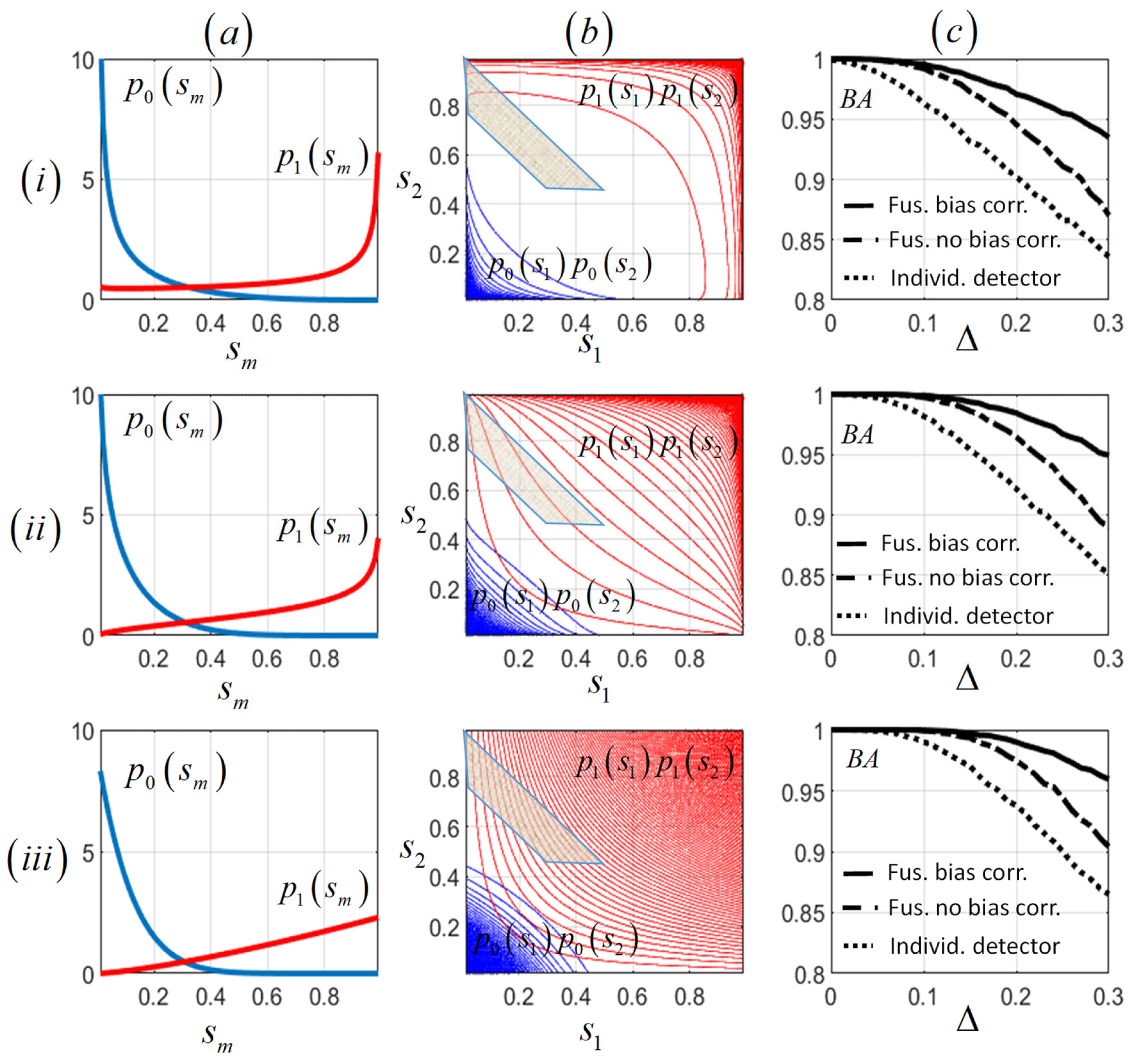Thus, in Figure 4a(i–iii), we have represented beta-PDFs, respectively, corresponding to $\alpha =0.4$, $\alpha =0.7$, and $\alpha =1.0$. In all three cases, the values ${\beta }_0$ and ${\beta }_1$ have been calculated to give biases $b_0=0.1$ and $b_1=0.3$. Note that each $\alpha$ parameter defines a different type of PDF, in any case appropriate to concentrate more probability to the left ($p_0\left(s_m\right)$) or to the right ($p_1\left(s_m\right)$) of the threshold of 0.5. As in Figure 3b, we have represented in Figure 4b(i–iii) the contour plots of $p_0\left(s_1\right)p_0\left(s_2\right)$ (blue) and $p_1\left(s_1\right)p_1\left(s_2\right)$ (red) considering, respectively, the conditional PDFs of Figure 4a(i–iii). We have marked in Figure 4b(i–iii) the shadowed area from Figure 2 where both bivariate PDFs have to be integrated to calculate the increase in $P{D}_z$ and $PF{A}_z$ due to bias correction. Once again, the distribution corresponding to the class $c=1$ expands more along the square, leading to a greater overlap with the shaded area. Then, we performed Monte Carlo simulations for the three $\alpha$ values, a unique value $b_0=0.05$ for class $c=0$ and a range of values $0.05\le b_1\le 0.35$ for class $c=1$, so that $0\le \Delta \le 0.30$. We have generated 10,000 samples from every required beta-PDF. Then, we have computed the balanced accuracies using (14), considering the MAP detector (2) for the individual scores, for the sum of the original scores and for the sum of the bias-corrected scores. Correction was implemented as indicated in (6) with sample estimates of the conditional biases $b_0$ and $b_1$. The results are shown in Figure 4c(i–iii). Similarly to the exponential case, an increase in bias reduces the balanced accuracy, while correcting for bias always produces the best result, with the relative improvement increasing with $\Delta$.

5. A Real Data Case

This section is devoted to evaluating the effectiveness of conditional bias correction in an automatic biomedical signal analysis problem to facilitate diagnosis. Two signal modalities and two classification methods will be considered. As we will see, this will open up the opportunity for 10 possible options, including unimodal classifiers and fusion of scores from two different modalities and/or two different classification methods.

The goal is to develop an automatic classifier for arousals [17,18] during sleep, as their frequency is correlated with the presence of apnea and epilepsy. An expert physician, through a thorough analysis of so-called polysomnograms, usually performs this classification manually: a set of different types of biomedical signals recorded during monitoring of the patient’s sleep. The record of arousal detections is called hypnogram. It is of obvious interest to use automatic hypnograms to alleviate the tedious and subjective task of the physician.

The polysomnograms were obtained from the public database Physionet [19]. In this experiment, we will consider the EEG and ECG signals recorded synchronously during patient sleep. Then, 8 EEG features and 12 ECG features were obtained, respectively, from the EEG and ECG signals in non-overlapped intervals of 30 sec. A total number of 10 patients were considered. The number of intervals varies for every patient, ranging from 749 (6 h and 14 min) to 925 (7 h and 42 min). The eight EEG features were powers in the frequency bands delta (0–4 Hz), theta (5–7 Hz), alpha (8–12 Hz), sigma (13–15 Hz), and beta (16–30 Hz), and three Hjorth parameters: activity, mobility, and complexity. These features are routinely used in the analysis of EEG signals [20,21,22]. The 12 ECG features were the following: autoregressive coefficients (4), Shannon’s entropy maximal overlap discrete wavelet packet transform at level four (4), and multiscale wavelet variance estimates up to fourth order using a Daubechies wavelet (4). More details on how to compute these features may be found in [23,24,25,26].

In this problem, class 1 corresponds to arousal and class 0 corresponds to any of the other possible sleep stages. We have considered two different classifiers. The first one is the Gaussian Bayes (GB), a generative classifier which assumes general Gaussian models for both $p\left(x/c=1\right)$ and $p\left(x/c=0\right)$, then the scores are calculated using

$$s={\displaystyle \frac{e^{-\frac{1}{2}\left({\left(\mathit{x}-{\mathit{\mu }}_1\right)}^T{\mathit{C}}_1^{-1}\left(\mathit{x}-{\mathit{\mu }}_1\right)\right)}}{e^{-\frac{1}{2}\left({\left(\mathit{x}-{\mathit{\mu }}_1\right)}^T{\mathit{C}}_1^{-1}\left(\mathit{x}-{\mathit{\mu }}_1\right)\right)}+e^{-\frac{1}{2}\left({\left(\mathit{x}-{\mathit{\mu }}_0\right)}^T{\mathit{C}}_0^{-1}\left(\mathit{x}-{\mathit{\mu }}_0\right)\right)}}},$$

(15)

where ${\mathit{\mu }}_0, {\mathit{\mu }}_1,{\mathit{C}}_0,{\mathit{C}}_1$ are the mean vectors and covariance matrices of the feature vectors, which have been estimated from the training data using maximum likelihood (ML) estimates. The second one is Logistic Regression, a discriminative method which computes the score using

$$s={\displaystyle \frac{1}{1+e^{-{\mathit{w}}^T\mathit{x}}}} .$$

(16)

There are different options for fitting the coefficient vector $\mathit{w}$; in our case, we opted for a closed form solution by solving an overdetermined system of linear equations. There exists an equation of the form ${\mathit{w}}^T\mathit{x}=\nabla$ for each instance $\mathit{x}$ of the training set, where $\nabla$ is a large positive number if $\mathit{x}$ belongs to $c=1$ or a large (magnitude) negative number if $\mathit{x}$ belongs to $c=0$. The classifiers were trained separately for every patient using the first half of the respective EEG or ECG recordings. Training includes the calculation of the conditional bias estimates ${\widehat{b}}_0$ and ${\widehat{b}}_1$ required by the proposed correction algorithm (5). The second half was then used for testing. The scores of all patients were grouped by class. Thus, each classifier generated a total of 6706 class 0 scores and 1708 class 1 scores.

We have considered ten options. The first four correspond to one modality–one classifier. The next two also consider one modality but the two classifiers are fused. Finally, the last four correspond to the fusion of the two modalities, either with the same classifier or a different one. Fusion is always implemented by simply computing the mean score.

Thus,

Table 1. Bias, probability of detection, probability of false alarm, and balanced accuracy of different options without bias correction. The best result without fusion and the best result with fusion are highlighted.

	−1 Modality −1 Method				−1 Modality −2 Methods (Fusion)		−2 Modalities −1 Method (Fusion)		−2 Modalities −2 Methods (Fusion)
OPTION	1	2	3	4	5	6	7	8	9	10
Modality and Method	EEG GB	EEG LR	ECG GB	ECG LR	EEG GB + EEG LR	ECG GB + ECG LR	EEG GB + ECG GB	EEG LR + ECG LR	EEG GB + ECG LR	EEG LR + ECG GB
Bias class 0	0.067	0.044	0.070	0.028	0.055	0.049	0.068	0.036	0.047	0.057
Bias class 1	0.291	0.355	0.354	0.439	0.323	0.396	0.322	0.397	0.365	0.354
Prob. of Detection (%)	70.86	64.01	64.60	55.94	68.05	59.92	70.10	64.31	69.69	65.24
Prob. of f. alarm (%)	5.76	4.03	5.67	1.95	4.40	2.82	4.92	1.83	3.65	2.80
Balanced Accuracy (%)	82.55	79.99	79.47	76.99	81.83	78.55	82.59	81.24	83.02	81.22

shows the results of the 10 options (numbered from 1 to 10) without applying bias correction. The conditional bias is shown as well as the balanced accuracy. Notice the bias is significantly higher for class 1 and that fusion does not reduce it (in fact, the bias after fusion is the mean bias). Also notice that fusion of GB + LR for one modality does not improve over using a single classifier for one modality. This is because of the high correlation between the scores of the same modality, as discussed later. The best balanced accuracy in Table 1 is obtained by option 9, which is the fusion of EEG GB + ECG LR, although the 83.02% obtained is only slightly greater than the 82.55% of the single modality EEG + GB.

Then,

Table 2. Bias, probability of detection, probability of false alarm, and balanced accuracy of different options with bias correction. The best result without fusion and the best result with fusion are highlighted.

	−1 Modality −1 Method				−1 Modality −2 Methods (Fusion)		−2 Modalities −1 Method (Fusion)		−2 Modalities −2 Methods (Fusion)
OPTION	1	2	3	4	5	6	7	8	9	10
Modality and Method	EEGb GB	EEGb LR	ECGb GB	ECGb LR	EEGb GB + EEGb LR	ECGb GB + ECGb LR	EEGb GB + ECGb GB	EEGb LR + ECGb LR	EEGb GB + ECGb LR	EEGb LR + ECGb GB
Bias class 0	0.020	0.016	0.024	0.009	0.018	0.016	0.022	0.012	0.014	0.020
Bias class 1	0.104	0.143	0.150	0.205	0.124	0.178	0.127	0.174	0.155	0.146
Prob. of Detection (%)	70.86	64.01	64.60	55.94	73.84	71.85	82.27	75.95	78.41	81.10
Prob. of f. alarm (%)	5.76	4.03	5.67	1.95	6.17	5.44	7.90	4.44	5.77	6.84
Balanced Accuracy (%)	82.55	79.99	79.47	76.99	83.84	83.21	87.13	85.75	86.32	87.18

shows the results corresponding to conditional bias correction. Notice that bias is clearly reduced in all options. The mean factor of reduction is 3 in class 0 and 2.5 in class 1. On the other hand, the balanced accuracy stays the same for the first four options as bias correction does not affect it when operating with individual detectors. However, the balanced accuracy increases in each of the six fusion options when compared with the corresponding option without bias correction. The best balanced accuracy is provided by option 10, which is very close to option 7. An improvement of 4.63% is achieved compared to the best case of Table 2.

To achieve statistical validation, we have repeated the previous experiments 100 times. In each repetition, a partition of the data set into two distinct halves was considered. In this way, we have obtained the mean and standard deviation of all the values shown in Table 1 and Table 2. The mean values are similar to the data in Table 1 and Table 2. The standard deviations never exceed 3% of the mean values.

We also performed significance tests on the balance accuracies obtained by bias correction in options 5 to 10, characterizing the distribution of the null hypothesis with the 100 balance accuracy values obtained with the corresponding option without bias correction. In all cases, the p-value was less than 0.05, so the null hypothesis is rejected, and we can consider that the balance accuracies from the bias correction are statistically significant.

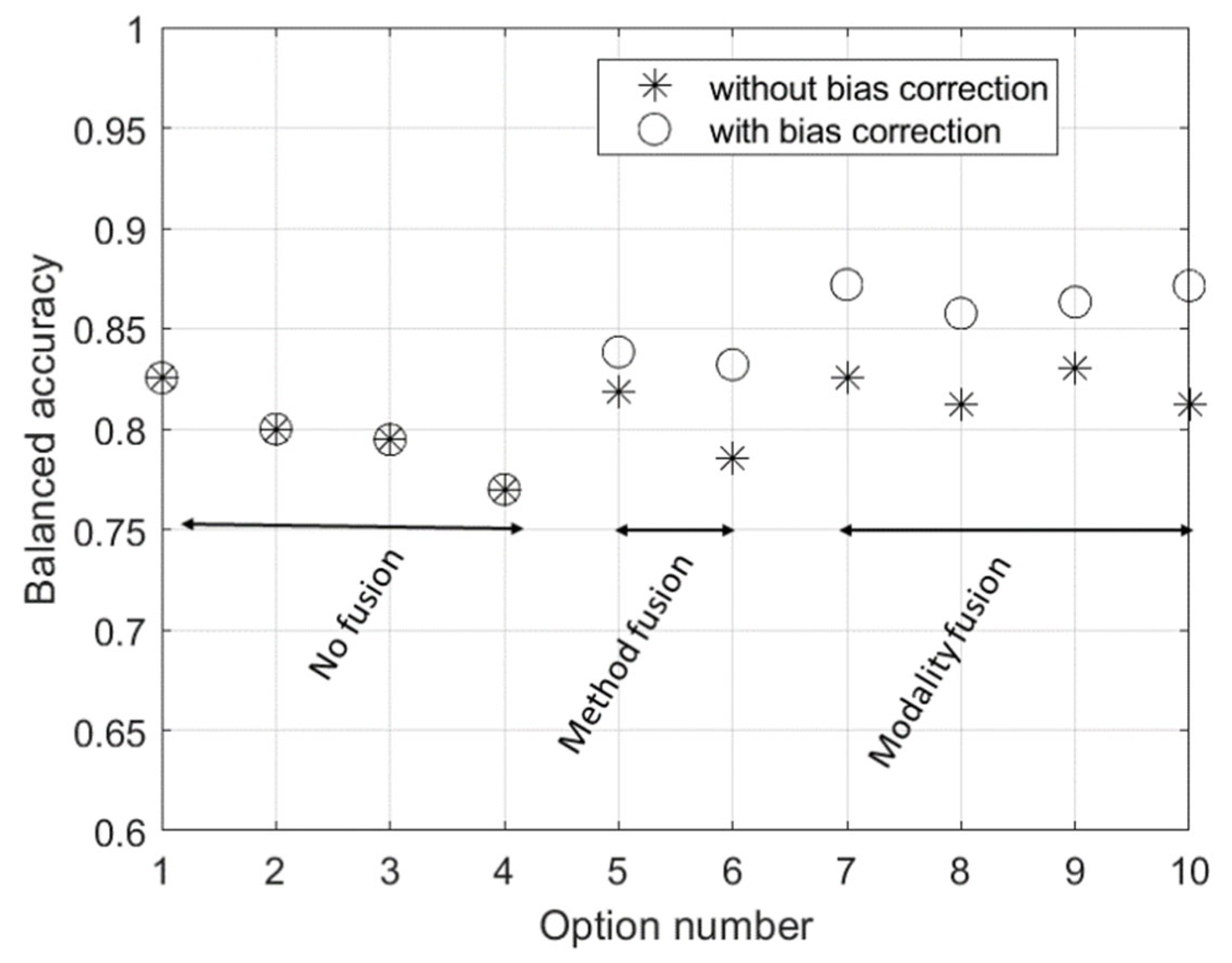
For better visualization, we have represented all the balanced accuracies from Table 1 and Table 2 together in Figure 5. It is clear that the fusion, in general, improves with respect to the use of a single detector; furthermore, the fusion of modalities improve with respect to the fusion of methods and fusion with bias correction improves with respect to fusion without bias correction.

The improved results of modality fusion can be explained in terms of the correlation between the fused scores. Note that in the previous theoretical developments, as well as in the simulations, we assumed uncorrelated scores. However, in real-world application, a certain degree of correlation can be expected, which will result in some deterioration in performance. It is expected that the correlation level between scores from different modalities should be lower than that from different methods applied to the same modality. This is because, if the modality is the same, the feature vector at the detector input will be the same regardless of the method used, resulting in a high correlation between the output scores. Changing the modality will reduce the output score correlation. This is shown in

Table 3. Correlation coefficients between the different sets of scores. The smallest correlation values are highlighted.

Class 0	EEG-GB	EEG-LR	ECG-GB	ECG-LR	Class 1	EEG-GB	EEG-LR	ECG-GB	ECG-LR
EEG-GB	1.00	0.61	0.32	0.26	EEG-GB	1.00	0.66	0.28	0.31
EEG-LR	0.61	1.00	0.20	0.30	EEG-LR	0.66	1.00	0.21	0.36
ECG-GB	0.32	0.20	1.00	0.44	ECG-GB	0.28	0.21	1.00	0.51
ECG-LR	0.26	0.30	0.44	1.00	ECG-LR	0.31	0.36	0.51	1.00

, where the correlation coefficients between scores for class 0 and class 1 are indicated. The minimum correlation coefficient in both classes corresponds to EEG-LR and ECG-GB, which coincides with the maximum balanced accuracy in Table 2.

In the experiments with real data in this section, as well as in the analyses and simulations in Section 3 and Section 4, we have always considered the MAP detector (threshold 0.5). This is convenient for potential extensions to the multi-class case, but it is not essential in the two-class case, where we could vary the threshold to adjust different operating points. In

Table 4. Balanced accuracy of the different options for different thresholds, with bias correction (BC) and with no bias correction (NBC). The best result for each threshold is highlighted.

		−1 Modality −1 Method				−1 Modality −2 Methods (Fusion)		−2 Modalities −1 Method (Fusion)		−2 Modalities −2 Methods (Fusion)
OPTION		1	2	3	4	5	6	7	8	9	10
Modality and Method		EEG GB	EEG LR	ECG GB	ECG LR	EEG GB + EEG LR	ECG GB + ECG LR	EEG GB + ECG GB	EEG LR + ECG LR	EEG GB + ECG LR	EEG LR + ECG GB
BA (%) threshold 0.40	BC NBC	83.23 83.23	81.28 81.28	79.64 79.64	78.06 78.06	85.24 83.56	84.20 81.99	87.38 86.96	86.59 84.32	86.44 85.91	87.39 86.59
BA (%) threshold 0.45	BC NBC	82.92 82.92	80.50 80.50	79.68 79.68	77.28 77.28	84.62 82.83	83.64 80.78	87.26 86.37	86.93 83.50	86.44 84.94	87.35 85.74
BA (%) threshold 0.50	BC NBC	82.55 82.55	79.99 79.99	79.47 79.47	76.69 76.69	83.84 81.83	83.21 78.55	87.13 82.59	85.75 81.24	86.32 83.02	87.18 81.22
BA (%) threshold 0.55	BC NBC	82.26 82.26	79.71 79.71	79.26 79.26	76.46 76.46	83.20 80.39	82.34 75.74	86.67 77.78	84.67 77.64	85.82 78.12	86.49 77.28
BA (%) threshold 0.60	BC NBC	82.04 82.04	79.38 79.38	78.98 78.98	76.67 75.67	82.61 79.56	81.24 74.86	85.51 76.55	83.91 75.35	85.20 76.03	85.81 75.40

, we reproduce the balanced accuracy results obtained with different thresholds for the 10 options from Table 1 and Table 2. A practical range of thresholds between 0.4 and 0.7 was selected, avoiding excessive false alarms for lower thresholds and low detectability for higher thresholds. We observe that the results maintain the improvement from bias correction and are consistent with what was observed in the previous results.

Thus, bias corrections do not affect individual detectors, while fusion with bias correction always provides improvement compared to fusion without correction. It is also observed that the relative improvement between correction and no correction increases as the threshold rises. This is explainable since the class with the highest bias was chosen as the class to detect, which means that corrections tend to raise the score values, with the impact of the correction becoming greater as the threshold increases.

6. Discussion

Let us discuss in terms of first principles. The optimum detector given $s_1$ and $s_2$ imply computation of the likelihood ratio ${\displaystyle \frac{p_1\left(s_1,s_2\right)}{p_0\left(s_1,s_2\right)}}$, which is to be compared with a given threshold. Unfortunately, most of the time, this only has theoretical interest because knowledge of the likelihood ratio is far from being realistic. Simple rules like computing the mean score (the one considered in this work) are much more useful yet reasonably grounded if the scores are considered as posterior probability of class $c=1$. However, it seems tentative to incorporate in the fusion rule any knowledge about the conditional PDFs which could be learned during training. Notice that assuming independence it is $p_i\left(s_1,s_2\right)=p_i\left(s_1\right)p_i\left(s_2\right)$, and biases $b_0$ and $b_1$ are respective statistics of $p_0\left(s_1\right)$ and $p_1\left(s_1\right)$ that are estimated during training and incorporated in the proposed method to improve the mean rule. Essentially, the method helps to resolve the situation in which both detectors make different decisions and the mean is below the threshold. This is achieved by increasing the value of the fusion statistic (the sum in our case) by the difference between the bias of the class to be detected and the bias of the other class. By defining the class to be detected as the one with the greatest bias, the difference will always be positive, which will increase both the probability of detection and the probability of false alarm. However, it is expected that the increase in detection probability will be more significant than the increase in false alarm probability, due to the fact that class $c=1$ has a greater bias, which implies uncorrected scores closer to the 0.5 threshold than those of class $c=0$.

An interesting point to discuss is that the analyses and simulations in Section 2, Section 3 and Section 4 assumed independence between the scores to be fused. To overcome this limitation, we should incorporate a score joint probability density model. Unfortunately, this could make the necessary analysis and/or simulations intractable. Notice that the chosen dependence model would still be an approximation, not necessarily appropriate for a real-world problem. Recently, it has been formally shown that the existence of correlation is one of the factors that can reduce the effectiveness of the fusion [16], so, in this sense, we can consider that the conclusions of Section 2, Section 3 and Section 4 set an upper limit on the performance achievable with the proposed method. Notice that in the real-world application of Section 5, the scores to be fused exhibit relatively high correlation values (Table 3), yet the bias correction proved effective, especially when the correlation is lower, as expected. Clearly, it would be valuable to investigate methods that reduce the correlation between the scores to be fused. For example, if different classifiers are involved in the fusion, different training subsets could be used for each classifier. Similarly, subsets recorded at different times for different modalities could be used for training. In any case, it would be advisable to analyze whether the improvement due to decorrelation outweighs the worsening due to the reduction in the effective size because of the partition of the whole training set into smaller subsets. Another approximation to the dependence problem could be devising more complex fusion methods that account for the possible correlation to obtain optimum solutions [16,27].

A line of research that also deserves further investigation concerns extending the method to the multi-class case. This extension is not always obvious in the field of machine learning. Frequently, the extension is carried out by decomposing the multi-class problem into a number of two-class problems. This approach can also be applied here, with everything considered in Section 2, Section 3 and Section 4 being directly applicable. Obviously, a global multi-class approach is always desirable. To this end, note that in the multi-class problem, each classifier generates as many scores as there are classes, which must satisfy the constraint of summing to 1. From training data, it is possible to determine the conditional biases of each of these scores, keeping in mind that the value to be estimated is 1 for the correct class and 0 for the rest of the classes. Corrections would be made, as in the two-class case, the class with the highest score is considered to be the “correct” one. One point to consider is that the corrected scores should sum to 1. We could, for example, correct all scores except 1, and adjust the uncorrected score so that they all sum to 1. In any case, extending the analyses in Section 3 and Section 4 to the multi-class case is not straightforward and requires significant additional effort.

Other possible lines of interest involve making a “soft” correction, for example, proportional to the score, thus taking into account the reliability of the decision made by the individual detector on the correct class.

Finally, other real-world data applications could be topics of future research.

7. Conclusions

Regarding the conclusions, we have shown that conditional bias is always greater than zero and that bias correction improves accuracy. However, we face an ill-posed problem since, strictly speaking, conditional bias correction requires prior knowledge of the true class. Nevertheless, we have shown that corrections can be made to the scores provided by each individual detector before fusion, using its own detections as true. Conditions for improvements have been derived theoretically, first in general and then for the exponential distribution case. Interest has also been demonstrated for the versatile beta distribution case, resorting to Monte Carlo simulations. Beta distribution is particularly well-suited for normalized random variables and allows for very different shapes of the class conditional PDF. Finally, a real data case was considered. We observed that the proposed method provides the best results, despite the different (more realistic) conditions of the real data with respect to the simplifying assumptions of the prior analysis.