Hybrid Deep Learning Approaches for Accurate Electricity Price Forecasting: A Day-Ahead US Energy Market Analysis with Renewable Energy

Abstract

Forecasting day-ahead electricity prices is a crucial research area. Both wholesale and retail sectors highly value improved forecast accuracy. Renewable energy sources have grown more influential and effective in the US power market. However, current forecasting models have shortcomings, including inadequate consideration of renewable energy impacts and insufficient feature selection. Many studies lack reproducibility, clear presentation of input features, and proper integration of renewable resources. This study addresses these gaps by incorporating a comprehensive set of input features, while these features are engineered to capture complex market dynamics. The model’s unique aspect is its inclusion of renewable-related inputs, such as temperature data for solar energy effects and wind speed for wind energy impacts on US electricity prices. The research also employs data preprocessing techniques like windowing, cleaning, normalization, and feature engineering to enhance input data quality and relevance. We developed four advanced hybrid deep learning models to improve electricity price prediction accuracy and reliability. Our approach combines variational mode decomposition (VMD) with four deep learning (DL) architectures: dense neural networks (DNNs), convolutional neural networks (CNNs), long short-term memory (LSTM) networks, and bidirectional LSTM (BiLSTM) networks. This integration aims to capture complex patterns and time-dependent relationships in electricity price data. Among these, the VMD-BiLSTM model consistently outperformed the others across all window implementations. Using 24 input features, this model achieved a remarkably low mean absolute error of 0.2733 when forecasting prices in the MISO market. Our research advances electricity price forecasting, particularly for the US energy market. These hybrid deep neural network models provide valuable tools and insights for market participants, energy traders, and policymakers.

1. Introduction

Electricity price forecasting (EPF) is essential for optimizing energy efficiency in the electricity market. Day-ahead electricity price forecasting, in particular, plays a vital role in maximizing the efficiency of power plants, optimizing financial gains, and reducing energy waste. Accurate predictions of day-ahead prices provide valuable insights for the economic operation of power plants, aiding in predicting future electricity load and preventing unexpected power outages. Short-term electricity price predictions are crucial for utilities and generation firms, enabling them to make informed decisions and maintain economic viability. Additionally, retailers and aggregators in emerging markets rely on their understanding of spot market pricing trends to thrive in the competitive energy market and sustain profitability. In this context, forecasting involves making predictions based on historical time series data, which often exhibit complex nonlinear relationships. A time series is a series of values of a quantity obtained at successive times, usually spanning equal intervals of time. Short-term forecasting, focusing on outcomes within seconds, hours, days, weeks, or months, holds practical significance [1]. Time series data often exhibit complex nonlinear relationships, prompting the application of various functions to explore the data with the specific objectives of modeling, extracting knowledge, and understanding the intricate dynamics between independent features and labels [2]. Time series models are commonly used to capture the linear characteristics of electricity pricing, but forecasting in this domain faces challenges due to the periodicity and volatility of power pricing [3,4]. In addition, the contribution of the rapid penetration of renewable energy is missing in the previous forecasting models. To address these challenges, an integrated machine learning model or a combination of models can be employed, encompassing data preprocessing, data cleaning, data preparation, data engineering and normalization, feature engineering, and artificial neural networks, as well as inclusion of renewable energy as features, offering a promising solution for electricity price forecasting. Our objective is to offer a comprehensive insight into the approach to energy price forecasting and emphasize the effectiveness of hybrid deep learning models in fulfilling the research goals.

The rest of this paper is organized as follows: Section 2 provides the problem statement, motivation, and our contribution through this research. Section 3 and Section 4 describe a day-ahead electricity market with a short description of the wholesale electricity market in the USA. A comprehensive literature review and related works are presented in Section 5. Section 6 elaborates on our research methodology with different hybrid approaches designed for this research. In Section 7, the proposed model architecture is illustrated. Data description, data preprocessing, feature engineering, etc., are described in Section 8 of this paper. Computational requirements and experimental setup are provided in Section 9. Validation matrices of the Hybrid ML models are presented in Section 10. The most important outcomes of this research, including model loss, model performance, and electricity price forecasting by our hybrid models, are discussed elaborately in Section 11, titled Result Analysis and Discussion. Section 12 presents our best-practice recommendations in the field of EPF. Finally, Section 13 concludes this research by summarizing the key findings and outlining potential future research directions.

2. Motivation and Contribution

2.1. Problem Statement

In recent years, the electricity market has witnessed a significant transformation due to the integration of renewable energy sources, advancements in smart grid technologies, and the increasing complexity of demand patterns. The renewable energy market, including sources like solar and wind power, has a significant impact on the American energy market. As a result, accurate and reliable forecasting of day-ahead electricity prices has become a crucial task for market participants, energy traders, and policymakers. Since electricity cannot be easily stored in large quantities, it must be generated in real time to meet demand. The US power grid, which connects approximately 145 million customers nationwide, comprises over 7300 power plants, nearly 160,000 miles of high-voltage power lines, as reported by the US Energy Information Administration (EIA, 2016) [5,6]. As of the year 2022, renewable energy sources accounted for around 24% of the nation’s electricity production due to the increasing demand for cleaner energy options [7]. The integration of renewable energy into the electrical network has made electricity price forecasting more challenging than ever before [8,9,10]. However, many previous studies have overlooked the influence of renewable energy sources, such as wind speed and weather temperature, as important features in their state-of-the-art forecasting models. Another significant issue in the electricity price forecasting market is the lack of sufficient information provided in research papers to ensure reproducibility. Common issues include the absence of details regarding the dataset used, lack of clarity on data preparation techniques (e.g., training–validation–test dataset splitting) [11,12,13,14,15,16,17,18], absence of input parameters used in the prediction models, and even the absence of data normalization, a critical preprocessing step prior to model training [19,20,21]. Traditional forecasting methods, such as statistical models, have provided valuable insights in the past, but they often struggle to capture the intricate nonlinear relationships and dynamic patterns present in electricity price data. In response to this challenge, the field of machine learning has emerged as a powerful tool for electricity price forecasting, leveraging its ability to model complex relationships and handle vast amounts of data. Some common issues at hand that revolve around electricity price forecasting in the context of the energy market are given below.

(i)

Training effective machine learning models requires large amounts of quality data. Unfortunately, accessing such data is frequently problematic because they are scarce. Previous research has struggled with this limitation, often having to work with limited datasets covering just a year or two.

(ii)

The performance and reliability of deep learning models can be compromised by poor data quality. When working with historical energy data, problems like noise, gaps in the data, and inconsistencies can lead to less accurate predictions.

(iii)

The growing adoption of renewable energy has made electricity prices more unpredictable and unstable.

(iv)

It is crucial to recognize what drives electricity production. While many studies have been criticized for using only 2–5 input variables, incorporating more diverse factors beyond price can significantly improve price forecasting accuracy.

(v)

Sequential data often have variable-length sequences, which can be challenging to handle using machine learning methods.

(vi)

Current prediction models, including neural networks, struggle to simultaneously capture both short-term and long-term patterns in electricity prices, reducing their forecasting accuracy.

(vii)

Models that memorize training data rather than learning true patterns will fail on new data. Testing performance on separate validation data helps identify whether a model has truly learned useful patterns or just memorized examples.

(viii)

Reproduction of existing research is important in machine learning to validate results, provide benchmarks for innovative approaches, educate researchers, and improve efficiency.

2.2. Our Research Contribution

This research aims to advance electricity price forecasting to bridge the research gap and overcome the challenges mentioned earlier. Our research endeavors to offer the following contributions:

(i)

We propose, design, and develop four state-of-the-art hybrid deep learning models to forecast electricity prices in the US energy market, namely, (a) VMD-DNN, (b) VMD-CNN, (c) VMD-LSTM, and (d) VMD-BiLSTM.

(ii)

Our dataset covers a 5-year period, providing enough data to effectively train the deep learning model. We also include data augmentation to create Supplementary Data.

(iii)

To ensure data integrity, we use VMD for denoising, apply spline interpolation to address missing data, and standardize the dataset with Z-score normalization to reduce discrepancies.

(iv)

To reduce volatility and uncertainty in price forecasting, we include temperature data to capture solar energy effects and wind speed data to account for wind energy’s impact on the electricity market.

(v)

We ensure the dataset is up-to-date, covering 2018 to 2022, to capture the impact of renewable energy integration on wholesale electricity prices.

(vi)

We include 24 time-sensitive input features to capture underlying patterns and enhance electricity price forecasting.

(vii)

We implement a sliding window technique to handle variable-length sequences, capture temporal dependencies, and optimize batch processing for training, validating, and testing the VMD-DL hybrid model.

(viii)

We validate our hybrid model using a separate validation dataset during training and apply mean squared error (MSE) to address the overfitting–underfitting issue, ensuring reliable model validation.

(ix)

We ensure transparency by detailing the data splitting process and making both our dataset and state-of-the-art model publicly available to support reproducibility of the research.

(x)

We deliver a set of best-practice guidelines in the field of electricity price forecasting.

3. Electricity Markets in the United States

The electricity market in the United States is a vital and intricate system that supports the nation’s energy needs. It operates regionally, with a combination of regulatory bodies and market participants ensuring a stable and affordable electricity supply. US electricity markets are classified into two main types: regulated and competitive. In regulated markets, integrated utilities are overseen by state or federal authorities, which control rates and investments. In contrast, competitive markets foster competition among power generators, allowing consumers to choose their electricity provider and enabling market-based pricing. The US electricity sector consists of both wholesale and retail segments. The wholesale market is critical for buying and selling electricity between generators, traders, and utilities, using mechanisms such as day-ahead, real-time energy markets, etc., to maintain reliability and balance. Initially, electricity is sold in wholesale markets before reaching consumers through retail markets, which vary in openness to competition or regulation. Figure 1 from eia.gov illustrates the US energy market structure [5]. The gray area shows regulated markets responsible for power generation, transmission, and distribution without competition. In contrast, competitive markets in regions like the Northeast, Midwest, Texas, and California are managed by independent system operators (ISOs) such as CAISO, MISO, SPP, ISO-NE, NYISO, ERCOT, and PJM [5,7]. These ISOs use competitive procedures to facilitate power exchange among independent producers and non-utility generators.

4. A Day-Ahead Electricity Market

The day-ahead energy market is a financial platform where participants buy and sell electricity by bidding on prices for the next day. It facilitates trades among generators, utilities, and energy traders to set the price for electricity delivery the following day. Participants submit bids based on projected supply and demand, taking into account factors like generation costs and market conditions. The market operator matches these bids to determine the clearing price, indicating the exchange price for electricity. This market helps participants manage risks, protect against price fluctuations, and make informed decisions about electricity generation and trading strategies.

5. Background Study

As electricity markets become more competitive, price forecasting has gained prominence due to the volatility of hourly prices, influenced by the dynamic nature of the market and advancements in renewable energy [22,23]. This volatility necessitates careful selection of input variables, model configuration, performance evaluation, and experimental setup for accurate forecasts.

Traditional time series and statistical methods have limitations in capturing the complex nonlinear relationships in electricity prices [24]. Consequently, machine learning techniques, particularly deep neural networks, have become popular for their ability to effectively model these nonlinear patterns [25]. However, single deep learning models often fail to fully capture diverse influencing factors like weather conditions, fuel prices, and renewable generation [25,26]. Hybrid models that integrate deep learning with other methods have shown promise. For example, Ali Agga et al. proposed a CNN-LSTM hybrid model that outperformed individual models in Morocco [27]. Jinliang Zhang et al. developed an adaptive hybrid model using variational mode decomposition, self-adaptive particle swarm optimization, seasonal autoregressive integrated moving average (SARIMA), and Deep Belief Networks for short-term electricity price forecasting [28]. In Canada, Daniel M. Jaimes et al. combined LSTM with XGBoost, achieving superior performance over benchmarks [29]. Despite these advancements, existing studies often lack a thorough analysis of energy market dynamics, renewable integration challenges, and reproducibility [30]. Thus, new hybrid deep learning architectures tailored to US market characteristics and renewable integration could improve forecasting accuracy. Recently, many models have emerged for electricity price projection, typically categorized into three main approaches:

(i)

Statistical models;

(ii)

Deep neural network models;

(iii)

Hybrid models.

5.1. Statistical Models

A statistical method involves extracting variation in a regressor variable using one that is orthogonal to unseen components of the target result [23]. These methods have been widely used in electricity price forecasting due to their simplicity, efficiency, interpretability, and ability to model time series properties and volatility. One of the earliest and most common techniques is the autoregressive integrated moving average (ARIMA) model, along with its variant, seasonal ARIMA (SARIMA). Contreras et al. demonstrated ARIMA’s effectiveness in forecasting electricity prices in Spain [31], while Conejo et al. enhanced ARIMA with wavelet transforms to better capture price volatility [32]. Recent advances in statistical methods for electricity price forecasting include linear regression, logistic regression, clustering, and tree-based approaches [33]. These models often use a linear combination of independent variables (regressors) to predict the dependent variable (electricity price). For example, in an hourly time series, this relationship is typically represented by Equation (1) as detailed below.

$$P_h=C_h{X}_h+E$$

(1)

where $C_h$ = [C₀, C₁,….. C_n] represents a row vector containing hourly coefficients, $X_h$ = [X₀, X₁,….. X_n]^T is a column vector of input features, and E is an error/bias term to calculate the hourly electricity price $P_h$.

Energy price forecasting has evolved to use LASSO (least absolute shrinkage and selection operator) regression for handling multiple inputs [34,35,36,37,38,39,40]. While ARIMA and GARCH (generalized autoregressive conditional heteroskedastic) models are also used in this domain [35,41], traditional statistical methods may miss complex patterns in big datasets. This leads to hybrid approaches that incorporate deep learning.

5.2. Deep Neural Network Models

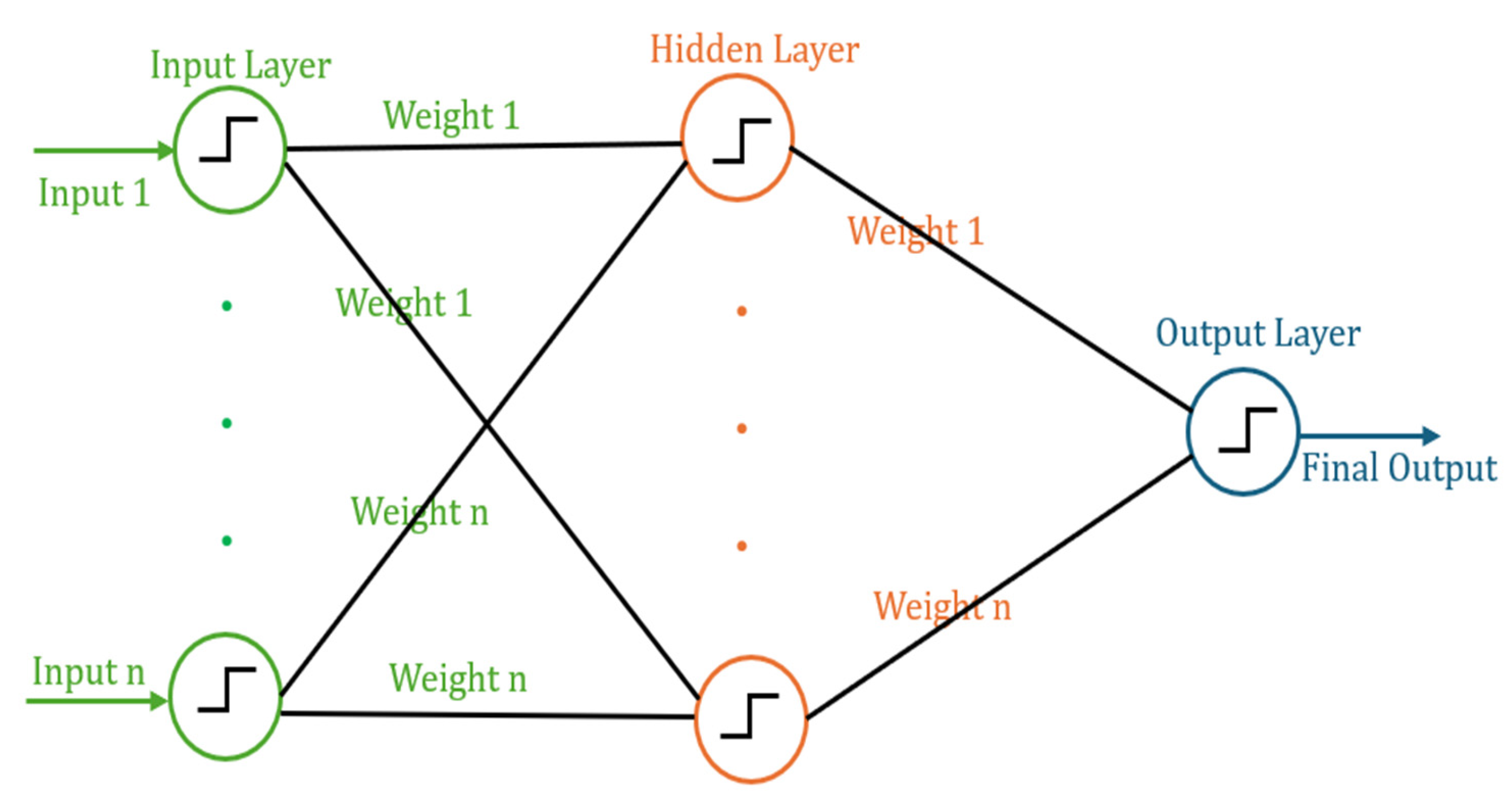
Deep learning models, particularly deep neural networks (DNNs), have become powerful tools for electricity price forecasting due to their ability to automatically learn complex nonlinear patterns from large datasets. Inspired by the human brain, artificial neural networks (ANNs) feature interconnected units (nodes) that mimic synapses, where connections (edges) and weights adjust during training to control signal flow. ANNs consist of three layers: an input layer that receives features, hidden layers that process the data, and an output layer that generates predictions. Their scalability and ability to handle large inputs make ANNs well-suited for complex systems [42]. Figure 2 illustrates the fundamental components common to most neural network models.

In day-ahead electricity price forecasting, deep learning models have significantly improved accuracy. The stacked denoising auto-encoder (SDA) model gained attention in 2016 for short-term predictions, while long short-term memory (LSTM) networks, a type of recurrent neural network (RNN), are widely used for capturing temporal dependencies in time series data [44,45,46,47,48,49,50]. Simple multi-layer DNNs and one-dimensional convolutional neural networks (CNNs) have also been applied to forecast hourly electricity prices [4,48,51,52,53]. While showing promise, these methods still need improvements in interpretability, uncertainty assessment, and domain knowledge integration.

5.3. Hybrid Models

There has been growing interest in hybrid and ensemble machine learning algorithms for electricity price forecasting. These models combine different techniques to leverage their respective strengths, often integrating statistical time series models with deep neural networks like CNNs, LSTMs, etc. Beyond neural networks, methods such as fuzzy logic, evolutionary algorithms, and expert systems have also been incorporated into hybrid models. Another popular hybrid method is the stacked or ensemble model, which merges multiple neural network models [24].

Hybrid models typically combine at least two of the three following modules: (i) data decomposition, (ii) feature selection, and (iii) statistical/neural network models for combined predictions [4,13,24,48,54,55,56,57,58,59,60,61,62,63,64,65,66]. Common decomposition techniques in energy forecasting include wavelet transform (WT), empirical mode decomposition (EMD), and variational mode decomposition (VMD). For feature selection, mutual information and correlation analysis are frequently used. These models consistently outperform individual approaches in complex regression tasks [67]. While hybrid models offer more advanced solutions for sophisticated problems, designing them effectively without adding unnecessary complexity remains a challenge.

6. Research Methodology

Based on extensive research, we propose a cutting-edge approach using a hybrid deep neural network model. This method combines variational mode decomposition (VMD) with various deep learning models, including deep neural networks (DNNs), convolutional neural networks (CNNs), long short-term memory (LSTM), and bidirectional LSTM (Bi-LSTM) networks. By integrating VMD with these architectures, the goal is to create a robust hybrid model for more accurate electricity price forecasting.

6.1. VMD

The variational mode decomposition (VMD) is a data augmentation technique that decomposes complex signals into a series of oscillatory components or modes. Since its introduction by Dragomiretskiy and Zosso in 2014, VMD has gained attention for its ability to disassemble multidimensional signals into independent frequency components [1,66,68]. This method partitions signals through an optimization process that minimizes correlation between modes while ensuring smoothness. VMD is particularly effective for analyzing nonlinear and nonstationary signals, such as electricity prices, by breaking them into intrinsic mode functions (IMFs), each with distinct temporal and spectral attributes [2,69].

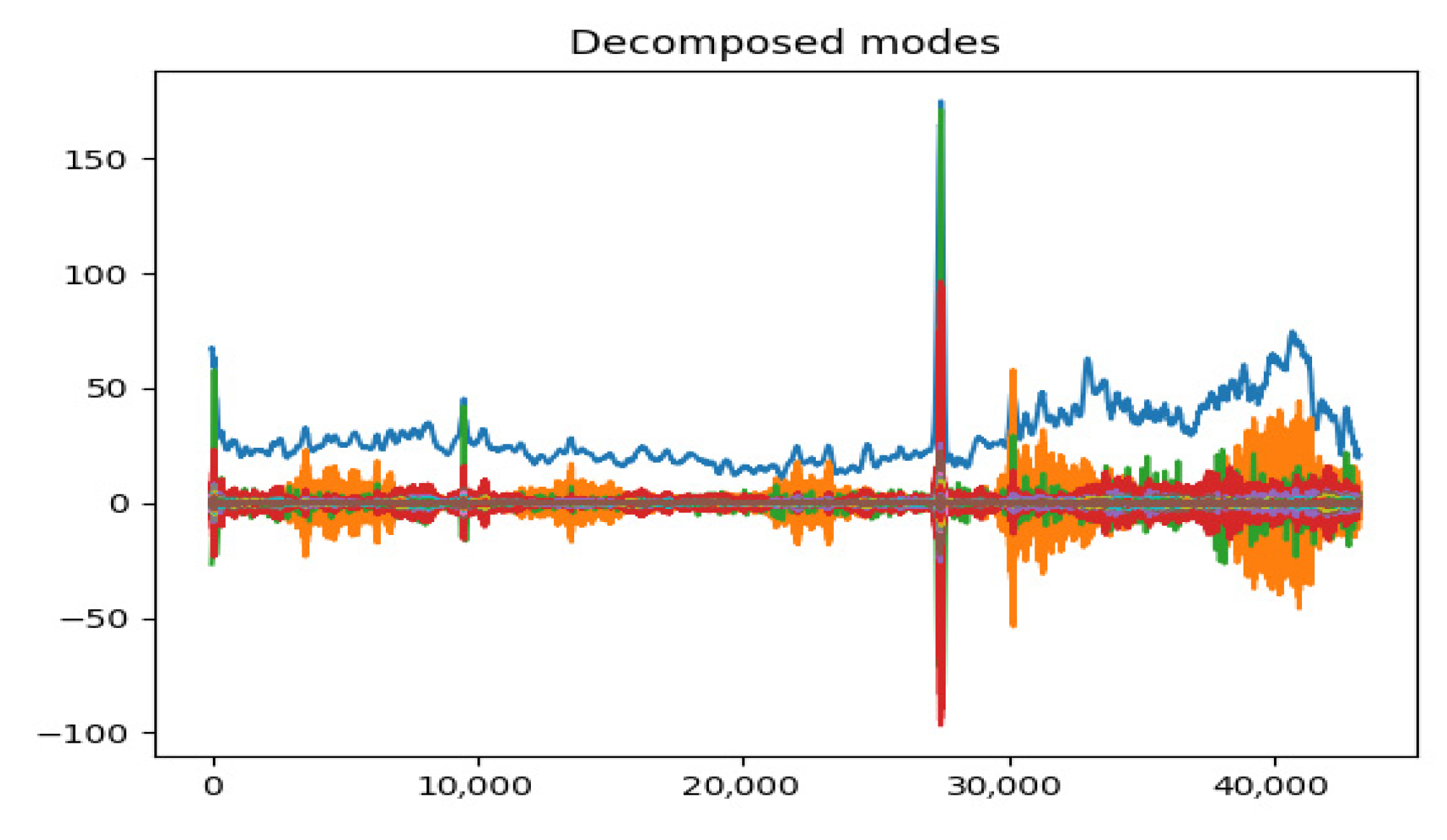
In our research, we applied VMD to decompose electricity price data into 12 sub-signals (IMF1 to IMF12), each representing a unique frequency component. These decomposed IMFs were treated as independent input features for the model, allowing it to capture the underlying patterns and dynamics more effectively, ultimately improving forecasting accuracy. The graphical representation in Figure 3 illustrates these decomposed signals overlaid on a single graph.

In the variational mode decomposition (VMD) process, several hyperparameters need to be set to control the decomposition. In this project, we have tuned data-fidelity constraint, dual ascent time step, the number of modes to recover, the parameter to determine if the first mode is fixed at zero frequency, the initialization method of mode frequencies, the convergence tolerance, etc. The input was a 1D time-domain signal that was decomposed using these parameters to ultimately produce 12 IMFs as signals shown in Figure 3.

6.2. DNN

Dense neural networks (DNNs), also known as feedforward neural networks or multi-layer perceptrons (MLPs), have proven highly effective for time series analysis, modeling complex nonlinear relationships and patterns in temporal data. DNNs consist of multiple fully connected layers, where each neuron in one layer is connected to every neuron in the next [70,71]. This structure allows them to handle high-dimensional inputs, capture both short- and long-term dependencies, and deal with noisy or incomplete data. DNNs typically include an input layer for sequential data, one or more hidden layers of densely connected neurons, and an output layer for predictions. Nonlinear activation functions, like ReLU or sigmoid, enable the network to learn complex patterns.

For this research, we designed a DNN architecture tailored for time series forecasting. The model includes an input layer to reshape multidimensional features, followed by three hidden layers with 32 neurons each using the ReLU activation. The output layer produces 24 forecasted values, providing an efficient framework for capturing temporal dependencies in electricity price data.

6.3. CNN

A convolutional neural network (CNN), typically used for image and video processing, can also effectively analyze one-dimensional time series data [72,73]. CNNs are known for their convolutional layers, which use filters or kernels to scan input data, detecting local patterns and dependencies [72,74,75]. This makes CNNs particularly powerful for time series analysis, where they can capture temporal features at various scales. They have been successfully applied in fields like financial forecasting, sensor data, and biomedical signals.

In this research, we implemented a 1D CNN with 256 neurons and the ReLU activation function. Additionally, we incorporated dense and reshape layers to process the input and generate output forecasts. The ability of CNNs to automatically extract features and capture local temporal dependencies makes them suitable for electricity price forecasting.

6.4. LSTM

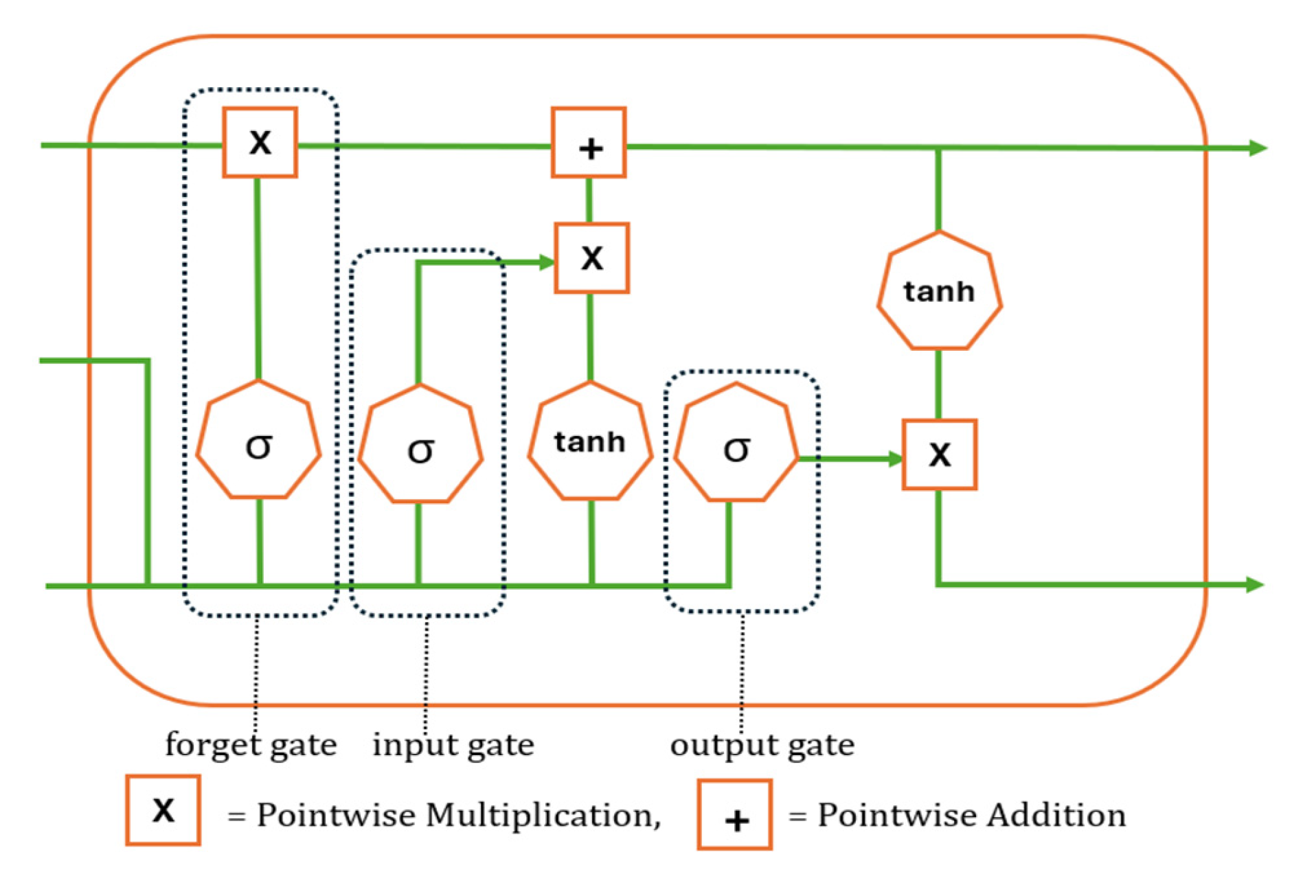
Long short-term memory (LSTM) is a deep learning neural network, a specialized type of recurrent neural network (RNN) designed to handle both long-term and short-term memory, removing the vanishing gradient problem seen in traditional RNNs [68,76,77,78]. LSTMs excel at identifying hidden patterns and continuously self-learn through gates and activation functions. A key feature is the LSTM cell, which replaces traditional hidden layers, containing an input gate, forget gate, and output gate to control the flow of information. The network operates through sigmoid layers, tanh layers, pointwise multiplication, and pointwise addition operations. Each LSTM cell comprises five layers, encompassing three sigmoid and two tanh layers. This structure enables LSTMs to capture long-term dependencies and also temporal patterns, especially in time series data.

In our setup, we used an input layer aligned with the sliding window method, an LSTM layer with 50 neurons, a 30% dropout layer to prevent overfitting, a dense layer for output extraction, and an output layer producing 24 forecasts. LSTM’s architecture makes it effective in capturing complex temporal patterns, such as electricity prices. Refer to Figure 4 for a basic diagram of an LSTM cell [78].

6.5. Bi-LSTM

Bidirectional long short-term memory (Bi-LSTM) enhances the traditional LSTM by processing input sequences in both forward and backward directions, allowing it to capture both past and future contextual cues. The Bi-LSTM framework consists of two LSTM layers: one handling the sequence forward and the other in reverse [79,80,81]. This dual-direction approach helps capture long-term dependencies and temporal patterns more effectively. The hidden states from these two layers can be combined either through concatenation or element-wise addition [7,72,74]. Refer to Figure 5 for an architectural depiction of the BiLSTM model.

In our research, the Bi-LSTM architecture included an input layer aligned with the sliding window method, a Bi-LSTM layer with 50 neurons, a 30% dropout layer to prevent overfitting, a dense layer with 64 neurons and ReLU activation, another dense layer for output extraction and channeled through a 1-dimensional tensor, and an output layer producing 24 forecasts. This bidirectional processing is especially useful for time series forecasting tasks, like electricity price prediction, where capturing intricate temporal relationships is essential.

7. Proposed Model Architecture

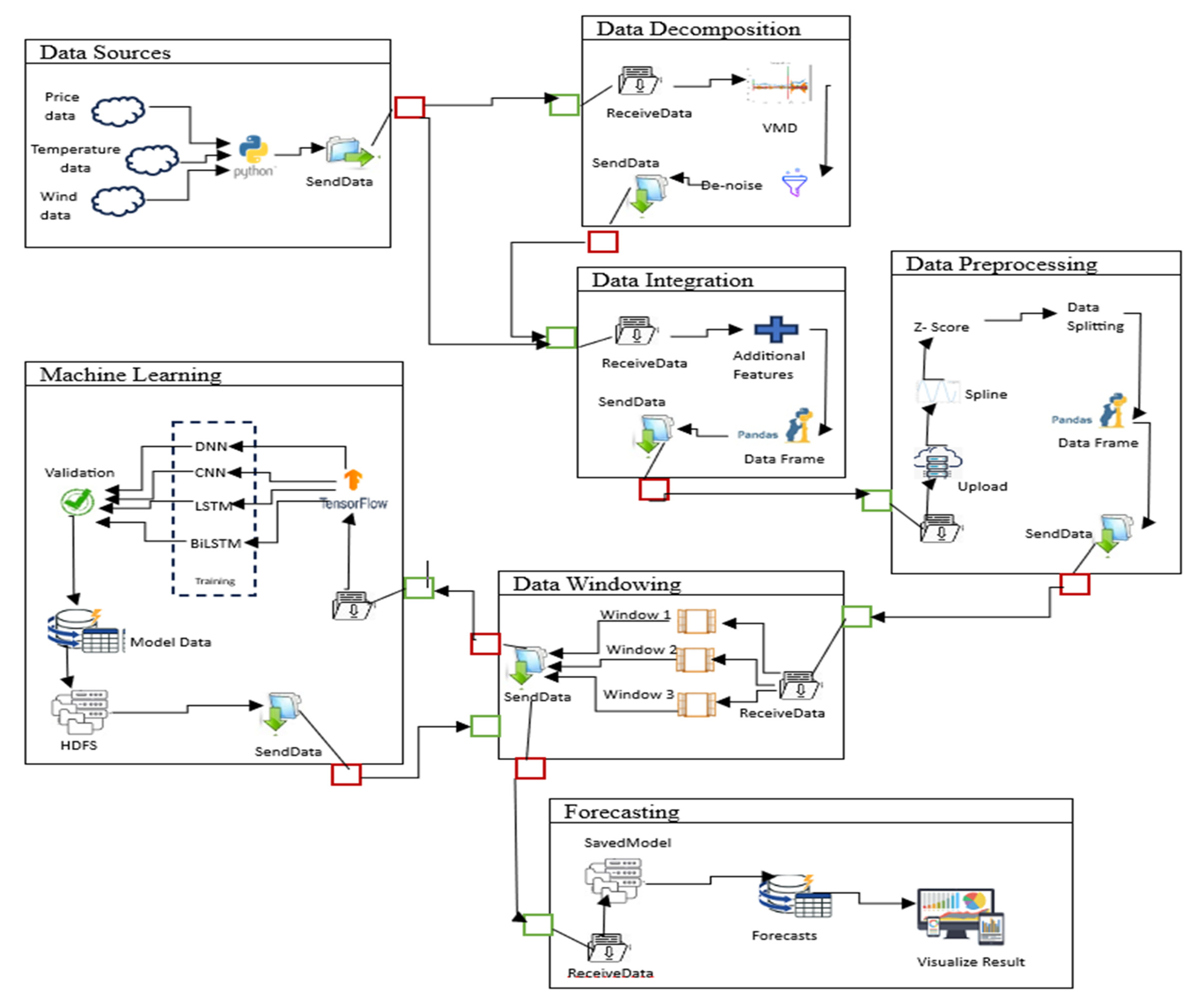
The hybrid approach for electricity price forecasting enhances accuracy, reliability, and adaptability by combining multiple deep learning methods. At the core of our system model is the deep learning hybrid model, which integrates four combinations of variational mode decomposition (VMD) with neural networks to capture both temporal and nonlinear relationships in the data. VMD is used for decomposing, filtering, denoising, and extracting features from electricity price data, while a deep learning(DL) model—either DNN, CNN, LSTM, or Bi-LSTM—is employed to train, validate, and test time series data using the MISO dataset.

To streamline training, we used a sliding window method with three time step combinations: 336 h, 168 h, and 24 h, to forecast the next 24 h. This technique optimizes the VMD-DL model during validation and generates electricity price predictions on test data. Figure 6 illustrates our VMD-DL framework for forecasting in the US energy market.

The proposed model architecture is structured using labeled boxes representing key system components, such as data sources, machine learning, etc. Each box contains subcomponents, with arrows indicating the data flow between them. All components, except for the ‘Data Source’ and ‘Forecast’ sections (which mark the start and end of the process), have subcomponents for receiving and sending data. The images or names used for subcomponents are carefully selected to accurately represent their functions. Red boxes indicate outgoing connections, while green boxes represent incoming ones. The model processes various input factors, including historical pricing data, demand shifts, weather conditions, temporal variables, and market indicators. These inputs are used during both the training and forecasting stages. The model is trained using the Adam optimization technique, and its performance is evaluated with appropriate metrics. This system generates up-to-date electricity price forecasts, providing valuable insights for decision-making in the energy sector.

8. Data Description and Preprocessing

Data is crucial for building accurate and reliable forecasting models, serving as the foundation for training, validation, and performance assessment. We provide an overview of the dataset and input features used in our electricity price forecasting study, offering a detailed description of its characteristics, quality, and implications for forecasting. To ensure replicable results, we follow these guidelines: (i) The dataset is publicly available. (ii) It is of sufficient length to allow thorough training of the deep learning model. (iii) It includes recent data to capture the impact of renewable energy on wholesale prices. We selected the MISO (Midcontinent Independent System Operator) market dataset, which fulfills these criteria. We also explain the input features, preprocessing steps, data flow, and data preparation involved in the study in the following sections.

8.1. MISO Market Data

The MISO (Midcontinent Independent System Operator) market covers the Midwest, parts of the South, and the Gulf Coast in the US, facilitating electricity trading among generators, utilities, and wholesale customers. To evaluate our hybrid neural network model, we used historical hourly electricity prices from MISO for training, validation, and testing, covering a five-year period from 1 January 2018 to 5 December 2022. This dataset is publicly available via platforms like misoenergy.org and energyonline.com [82,83]. Although MISO includes eight regional HUBs, our study focuses on the Minnesota HUB (MINN.HUB) for simplicity. Figure 7 presents the day-ahead electricity price series from the MISO dataset, illustrating the local marginal price (LMP) against hourly time steps within the specified timeline. This figure also reveals that MISO market prices remain mostly positive, with occasional zero values and frequent price spikes. This dataset was used as a 1-D time series input to generate 12 decomposed IMFs, as explained in Section 6.1. To account for the influence of wind and solar energy on power generation, the dataset also includes hourly temperature and wind speed data for Minnesota. In this study, our selection of temperature and wind speed as environmental inputs was guided by both data availability and their direct relevance to solar and wind energy generation, two of the most prominent renewable sources in the US electricity grid. These weather variables, sourced from the ASOS Network of Iowa State University, are publicly available [84]. The temperature and wind speed data were collected for the same time period as the MISO day-ahead price data to ensure alignment with the electricity price forecasting model.

8.2. Feature Selection

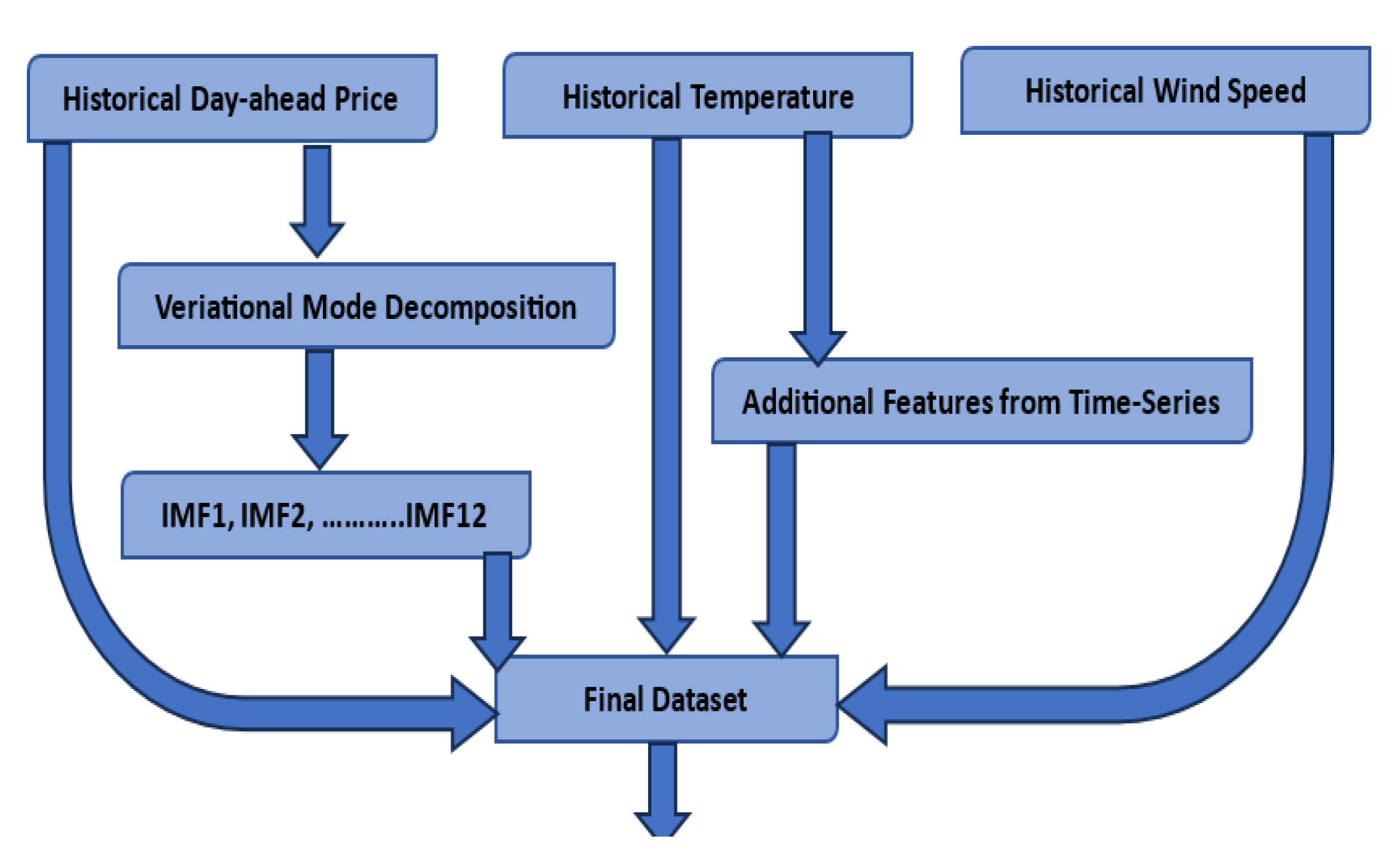
In time series analysis, the input features are crucial for a deep learning (DL) model as they help extract valuable patterns from the data, significantly impacting the model’s forecasting capabilities. The careful selection of these features enhances the model’s performance. Figure 8 illustrates the feature generation and selection process for electricity price forecasting of this project. As shown in the figure, in addition to price, temperature, wind, and decomposed IMFs, 10 derived time-sensitive features were generated as additional features from the specified time series data. In this study, the following input features were used to forecast 24 h of day-ahead electricity prices:

(i)

Hourly historical day-ahead electricity prices ($);

(ii)

Hourly historical temperature (°F);

(iii)

Hourly historical wind speed (mph);

(iv)

Twelve decomposed signals from historical prices (IMF 1–12);

(v)

Weekday/weekend identification (weekdays = 0, weekends = 1);

(vi)

Hour of the day (0–23);

(vii)

Day of the week (0–6);

(viii)

Day of the month (1–28/30/31);

(ix)

Month of the year (1–12);

(x)

Midweek/non-midweek (Tue/Wed/Thu = 1, others = 0);

(xi)

Daily sine signal for the time series;

(xii)

Daily cosine signal for the time series;

(xiii)

Yearly sine signal for the time series;

(xiv)

Yearly cosine signal for the time series.

A total of 24 input features were used in the hybrid deep neural network model. The complete dataset with 24 features is publicly available at my Kaggle repository (https://kaggle.com/datasets/ec366402ad42f42148a85b457bf95ce668111b92e14d8acdf3d32c3f1c95ee13 accessed on 3 August 2025).

8.3. Data Interpolation

Data interpolation is essential for preparing time series data for deep learning (DL) models, as it fills in missing or incomplete data points, creating a continuous dataset. This process estimates absent values based on existing information, maintaining the temporal coherence of the time series and ensuring a seamless sequence for the DL model’s training and analysis [85]. In this research, we used spline interpolation to handle missing data points and smooth extreme price spikes. This method divides the dataset into smaller segments, fitting a piecewise continuous curve to each segment, known as splines. These splines connect polynomial equations smoothly at specific data points or knots, making them ideal for interpolating data with noise or irregularities. The smoothness of splines prevents abrupt changes between consecutive points, making them effective for managing irregular data distributions and aiding in denoising by providing reliable estimates between data points.

8.4. Data Normalization

Data normalization, or feature scaling, is a preprocessing technique used in deep learning (DL) to standardize input data to a common scale. It is essential for data preparation before training neural networks, as it adjusts input feature values to have similar magnitudes and distributions. This process improves convergence, stability, and overall performance during training, especially for heterogeneous data. In this research, we employ Z-score normalization to manage outliers and data by subtracting the mean from the data points and dividing by the standard deviation. The mean and standard deviation are calculated using only the training data to ensure that validation and test sets remain unaffected, optimizing the model’s accuracy. Equation (2) illustrates the Z-score normalization applied to each data point in the dataset [86].

Z-score = (x − μ)/σ

(2)

where x = original value, μ = mean of the dataset, and σ = standard deviation of the dataset.

8.5. Data Windowing

Data windowing is a crucial step in training deep learning models for time series analysis. This method entails dividing the time series data into smaller windows or subsequences to facilitate training, validation, and testing. Each window consists of a consecutive sequence of data points, allowing the model to identify localized patterns and temporal relationships within the data [87]. By leveraging the temporal order of the data and enhancing the model’s ability to detect localized patterns, data windowing enables the deep learning model to process and learn from the segmented windows effectively. In this research, we employed three distinct window sizes to explore different strategies for capturing underlying trends in time-series data. Specifically, we utilize window sizes of 15 (14 + 1) days, 8 (7 + 1) days, and 2 (1 + 1) days for training, validation, and testing our hybrid model. Additional insights into the specific data points considered for each windowing technique are provided in

Table 1. Data windowing technique.

Techniques	Previous Hours	Forecasting Hours	Total Window Size
Window 1	336 (14 days/2 weeks)	24 (1 day)	360 h (14 + 1 days)
Window 2	168 (7 days/1week)	24 (1 day)	192 h (7 + 1 days)
Window 3	(1 day)	24 (1 day)	hours (1 + 1 days)

.

8.6. Data Preparation

Machine learning models typically require three distinct datasets for conducting experimental analysis. These are (i) the ‘train dataset’ for model training, (ii) the ‘validation dataset’ for assessing model quality, and (iii) the ‘test dataset’ for evaluating the model post-validation. In this research, the training dataset comprised the initial 34,920 h, spanning from 1 January 2018 to 25 December 2021. The validation dataset extended from 26 December 2021 to 20 September 2022, encompassing 6456 h of data. Finally, the test dataset covered the period from 21 September 2022 to 4 December 2022. Notably, the data were not randomly shuffled during splitting to preserve the sequence within the dataset.

Table 2. Data splitting on MISO market data.

Dataset Name	Start Date	End Date	Hours
Training	1 January 2018	25 December 2021	34,920
Validation	26 December 2021	20 September 2022	6456
Test	21 September 2022	12 April 2022	1800

provides a detailed description of the data splitting process applied to our MISO dataset.

9. Computational Efficiency and Experimental Setup

The experimental setup for our research project was meticulously crafted to ensure the robustness and reliability of our analysis, particularly in the domain of electricity price forecasting. To address the computational challenges inherent in deep learning models, particularly regarding efficiency, we harnessed the power of GPU acceleration, specifically leveraging NVIDIA T4 Tensor Core GPUs for expedited training speeds and reduced computational costs [88]. Following model training using the training dataset, we evaluated the model’s performance using the validation dataset, and fine-tuning hyperparameters as needed. The complete experimental setup required the following technology and algorithms:

• Machine Learning Framework: TensorFlow 2.0;
• Programming Language: Python 3, Pandas 2.3, NumPy 2.3, Matplotlib 3.10, Seaborn 0.13;
• Processing Unit: GPU (NVIDIA T4 Tensor Core) [88];
• Notebook: Google CoLab;
• Dataset Market: MISO;
• Dataset Length: 5 years;
• Total Inputs: 24 input features;
• Data Augmentation: VMD;
• Data Interpolation Method: Spline;
• Data Normalization Method: Z-score;
• Data Splitting: Training, Validation, and Test;
• Window Sliding Method: (i) Window 1 (14 + 1 days), (ii) Window 2 (7 + 1 days), and (iii) Window 3 (1 + 1 days);
• Deep Learning Neural Network: VMD, DNN, CNN, LSTM, and BiLSTM;
• Optimization Algorithms: Adam;
• Model Validation and Performance Matrices: MSE, MAE;
• Forecasting Timeframe: 24 h.

Table 3. Model summary.

Model Name	Model Summary
VMD-DNN	5-layer network, batch size 336 (varies depending on window type), Adam optimizer, learning rate 0.001, ReLU activation, and a total of 259,928 trainable parameters
VMD-CNN	4-layer network, batch size 336 (varies depending on window type), Adam optimizer, learning rate 0.001, ReLU activation, and a total of 1,984,792 trainable parameters
VMD-LSTM	4-layer network, batch size 336 (varies depending on window type), Adam optimizer, learning rate 0.001, ReLU activation, and a total of 16,224 trainable parameters
VMD-BiLSTM	4-layer network, batch size 336 (varies depending on window type), Adam optimizer, learning rate 0.001, ReLU activation, and a total of 38,024 trainable parameters

summarizes the architectural details of the proposed hybrid deep learning models used in this study. Each model integrates variational mode decomposition (VMD) with a specific deep learning framework—DNN, CNN, LSTM, or BiLSTM. All models utilize the Adam optimizer with a learning rate of 0.001 and employ ReLU as the activation function. ReLU activation was chosen due to its computational efficiency and effectiveness in handling nonlinear relationships in deep learning models. In our experiments, ReLU enabled faster convergence during training and improved generalization by reducing the likelihood of vanishing gradients. Its simplicity also contributed to stable and scalable learning across all proposed VMD-based deep learning architectures and is well-suited for time series forecasting tasks like electricity price prediction.

10. Model Validation Matrices

In electricity price forecasting, the primary metrics employed to gauge forecast accuracy include mean absolute error (MAE) and mean squared error (MSE). During the training phase of our deep learning (DL) model, we utilized MSE as a loss function to quantify the loss, while MAE was employed to compute the forecast errors generated by the model.

10.1. MSE

Mean squared error (MSE) serves as a widely adopted metric for assessing the loss function of a deep learning model. It is employed to assess the model’s loss on both training and validation datasets. MSE is calculated by squaring the differences between predicted and actual values, followed by averaging across the dataset [89]. The squared differences emphasize larger errors, making it particularly useful for capturing the magnitude of errors in regression tasks. Equation (3), provided below, outlines the computation for MSE.

$$MSE={\displaystyle \frac{1}{n}}\sum _{i=1}^n{\left(y_i-{\widehat{y}}_i\right)}^2$$

(3)

where n = total data points, y = original electricity price, and y-hat = forecasted price by VMD-DL hybrid model.

10.2. MAE

The mean absolute error (MAE) is extensively utilized within electricity price forecasting to gauge the accuracy of price predictions. In calculating MAE, the absolute disparities between predicted and actual values are tallied, then averaged across the dataset [90]. These absolute differences furnish an indication of the average magnitude of errors in the forecasts. Unlike the squared differences utilized in the mean squared error (MSE), MAE does not amplify the influence of outliers or substantial errors. Consequently, MAE exhibits greater resilience to extreme values and outliers, rendering it applicable for scenarios where such data points are expected. The error computation is delineated by Equation (4) [90].

$$MAE={\displaystyle \frac{1}{n}}\sum _{i=1}^n|\mathrm{ }{X}_{i-real}-\mathrm{ }{X}_{i-forecasted}\mathrm{ }|$$

(4)

Here, n = total of hours, X_real = original price, and X_forecasted = forecasted price by the VMD-DL hybrid model.

11. Result Analysis and Discussion

Electricity price forecasting is one of the most critical issues in the economic operation of the power system. High accuracy in the day-ahead price prediction can increase the profitability of the wholesale electricity market. Our hybrid models on MISO market data show ignorable error and impressive performance on electricity price forecasts. In this section, we present the results of the state-of-the-art VMD-DL hybrid deep learning model on the MISO dataset. To deploy the VMD-DL hybrid model, we created four different combinations, namely, (i) VMD-DNN, (ii) VMD-CNN, (iii) VMD-LSTM, and (iv) VMD-BiLSTM.

11.1. Model Loss

Loss functions quantify the discrepancy between predicted and actual values and serve as optimization objectives during model training and validation of the model. We chose MSE as a measure of the quality of the model. The values are always non-negative, and the ones closer to zero are always better for MSE. Figure 9a–d show the model loss during the training and validation process by each of the four hybrid model combinations. The x-axis represents 50 epochs of training and validation by the hybrid model, and the y-axis represents the loss on each epoch. The loss figure shows that the training loss and validation loss of each of these models are closer to zero. This ensured that this model was neither underfitting nor overfitting; rather, the fitting with the given dataset was within an acceptable range.

The overall loss values during the training and validation period by our three different windowing techniques and four different combinations of hybrid models are presented in

Table 4. Model loss by different windowing techniques and hybrid models.

Window Techniques	Hybrid Model	Model Loss (MSE)
Window 1 (14 + 1 days)	VMD-DNN	0.3312
	VMD-CNN	0.2637
	VMD-LSTM	0.1796
	VMD-BiLSTM	0.1517
Window 2 (7 + 1 days)	VMD-DNN	0.2824
	VMD-CNN	0.1956
	VMD-LSTM	0.1730
	VMD-BiLSTM	0.1318
Window 3 (1 + 1 days)	VMD-DNN	0.1229
	VMD-CNN	0.1418
	VMD-LSTM	0.1590
	VMD-BiLSTM	0.1236

. We have found that for Window 1, when we considered 14 previous days to forecast 1-day-ahead electricity prices, the model’s overall loss by VMD-DNN was 0.3312, the loss by VMD-CNN was 0.2637, the loss by VMD-LSTM was 0.1796, and the loss by VMD-BiLSTM was only 0.1517. All of these loss values are ignorable and significantly indicate a good result by each of these hybrid models. However, in our study, the VMD-BiLSTM model demonstrated superior performance compared to the other three models in all window implementations.

11.2. Model Performance

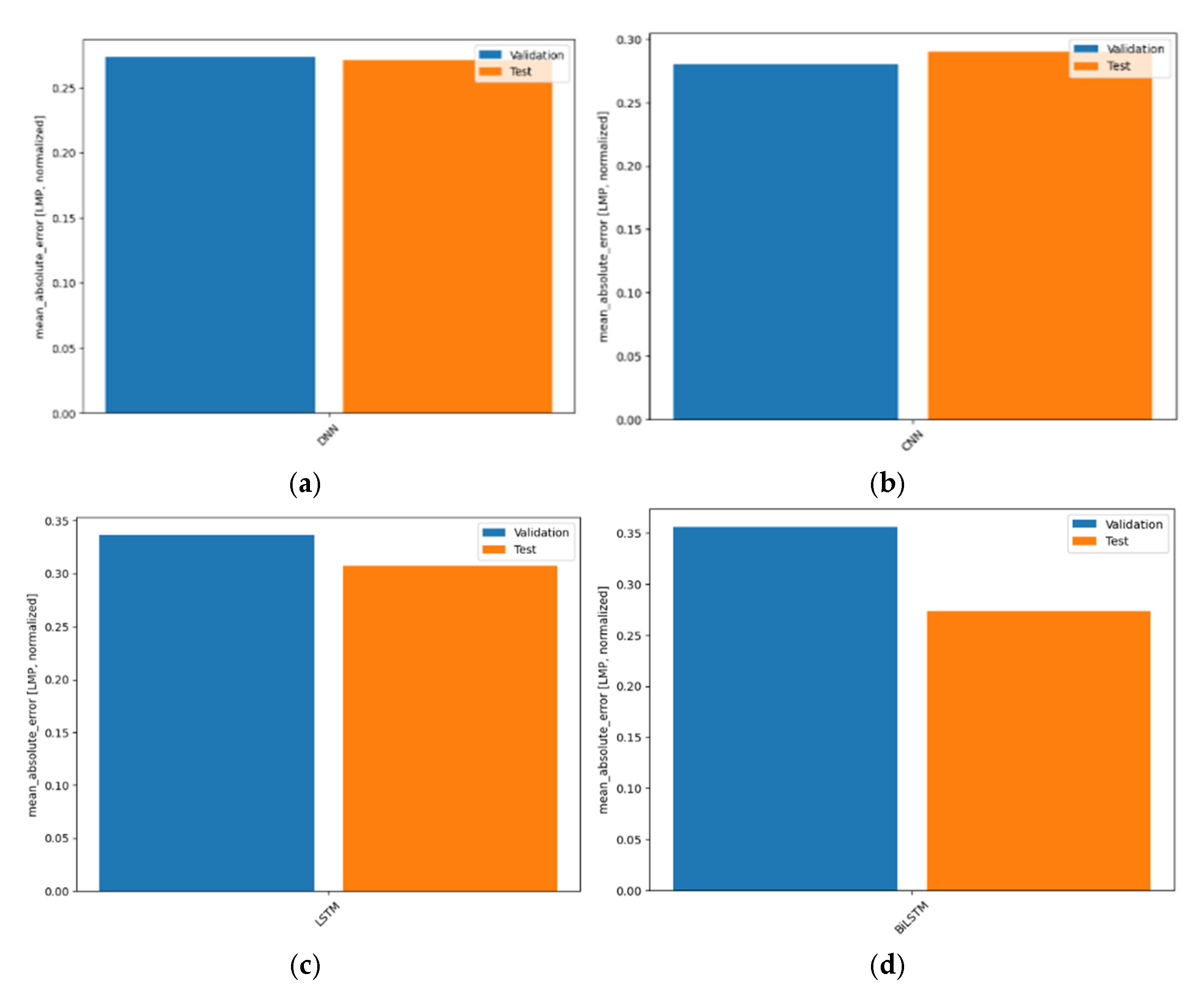
Machine learning model performance refers to the evaluation and measurement of how well a deep learning model performs in achieving its intended task or objective. It is important to note that DL model performance is not solely determined by the model architecture but also influenced by factors such as the quality and representativeness of the training data, the availability of labeled or ground truth data for evaluation, and the choice of appropriate hyperparameters and optimization algorithms during model training. The Mean absolute error (MAE) is one of the most frequently employed metrics in the field of electricity price forecasting to assess the precision of price forecasts. A lower error means high accuracy in price prediction. Figure 10a–d show the model performance on the validation and test datasets by each of the four hybrid model combinations. The MAEs for each of these hybrid models were almost equal and very close to each other on the validation dataset and the testing dataset.

The MAEs on the test dataset by the three different windowing techniques and the four different combinations of hybrid models are presented in

Table 5. Model performance by different windowing techniques and hybrid models.

Window Techniques	Hybrid Model	Model Performance (MAE)
Window 1 (14 + 1 days)	VMD-DNN	0.4623
	VMD-CNN	0.4083
	VMD-LSTM	0.3312
	VMD-BiLSTM	0.3014
Window 2 (7 + 1 days)	VMD-DNN	0.4161
	VMD-CNN	0.3472
	VMD-LSTM	0.3238
	VMD-BiLSTM	0.2782
Window 3 (1 + 1 days)	VMD-DNN	0.2710
	VMD-CNN	0.2930
	VMD-LSTM	0.3077
	VMD-BiLSTM	0.2733

. We found that for Window 1, when we considered 14 previous days to forecast 1-day-ahead electricity prices, the model’s MAE by VMD-DNN was 0.4623, the MAE by VMD-CNN was 0.4083, the MAE by VMD-LSTM was 0.3312, and the MAE by VMD-BiLSTM was only 0.3014. All of these MAE values are ignorable errors and significantly indicate a high accuracy in price forecasting by each of these hybrid models. However, in our study, the VMD-BiLSTM model demonstrated superior performance compared to the other three models in all window implementations.

11.3. Electricity Price Forecasting Using Hybrid Models

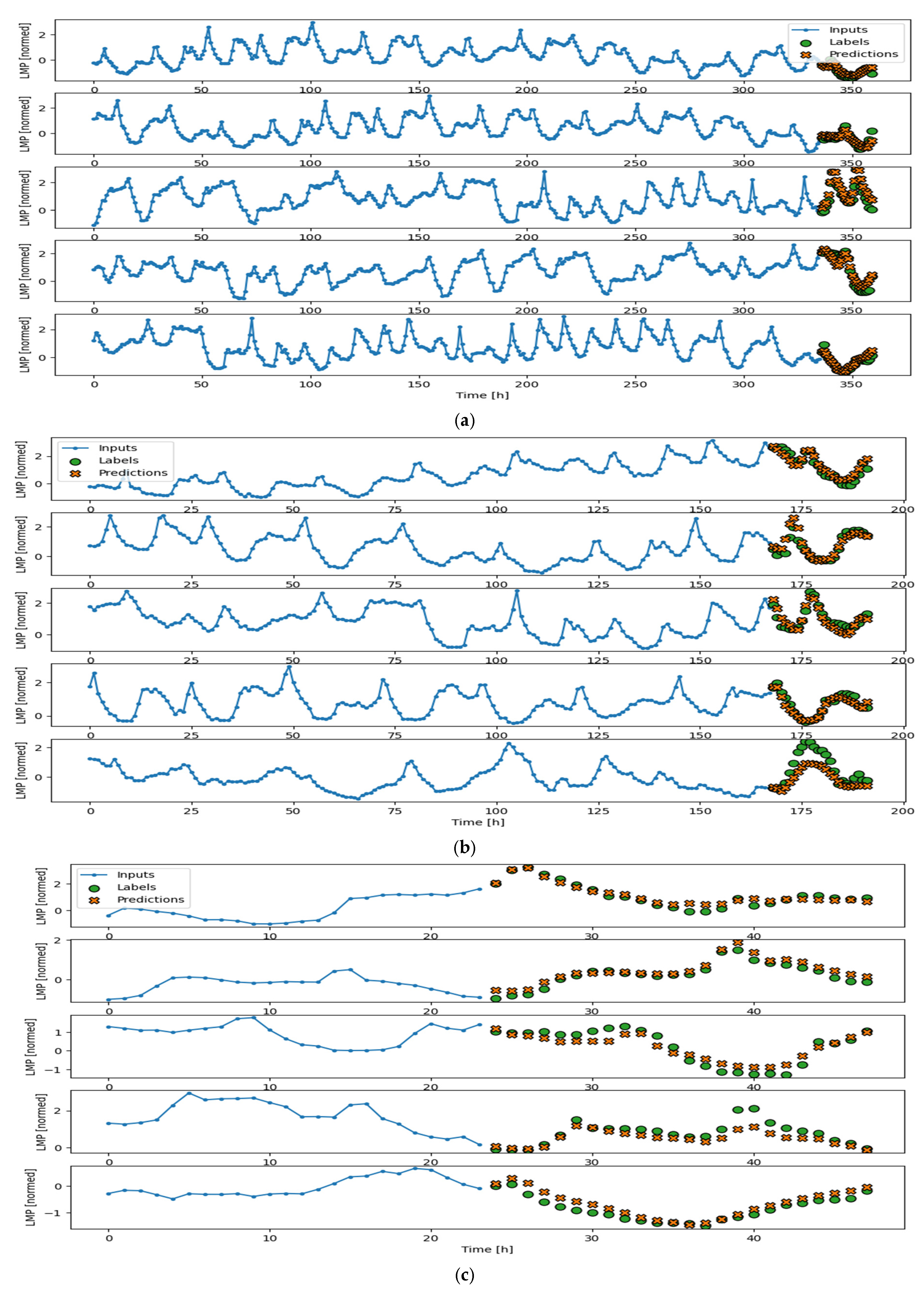
In this Section, we delve into the electricity price predictions made by the VMD-DL models on our designated test dataset. As previously mentioned, we have formulated four hybrid model combinations like the following: (i) VMD-DNN, (ii) VMD-CNN, (iii) VMD-LSTM, and (iv) VMD-BiLSTM. Within each hybrid model, we present three figures, each with five subplots representing five random windows.

In each of the following figures, the blue portion has a different length depending on the window size. This can be of three kinds: (a) the length of Window 1 is the previous 336 h (14 days) of price, (b) the length of Window 2 is the previous 168 h (7 days) of price, and (c) the length of Window 3 is the previous 24 h (1 day) of price. The green circles are 24 h (1 day) of original data labels, and the orange cross is 24 h of forecasted price by the four hybrid models. The green circles and orange forecasts have the same length, i.e., 24 h for all three windowing techniques. To keep things simple and concise, we are only including the forecasting figures for our best model. Figure 11 ((a) Window 1, (b) Window 2, and (c) Window 3) displays the predicted outcomes for hourly electricity prices by the VMD-BiLSTM hybrid model on five randomly selected days from the test dataset. These visual representations demonstrate the remarkable adherence of the price prediction to the underlying trend, indicating strong forecasting capabilities of this hybrid model within the MISO energy market.

Through this comprehensive result analysis and model validation process, we aim to provide a thorough evaluation of our electricity price forecasting models. The insights gained from this analysis enable us to assess the practicality and reliability of the models in real-world scenarios, offering valuable guidance for decision-makers in the energy market.

12. The Best Practices in Electricity Price Forecasting

US electricity markets are evolving to accommodate changing energy landscapes, emerging technologies, and environmental considerations. The pursuit of a reliable, affordable, and sustainable electricity supply remains a top priority, driven by market forces, regulatory policies, and the collective goal of achieving a clean energy future. This research aims to explore the intersection of renewable energy and electricity price forecasting using hybrid deep learning models. We aim to investigate the impact of incorporating different DL architectures, such as DNNs, CNNs, LSTMs, and BiLSTMs, in hybrid models for electricity price forecasting. Based on the extensive comparison of electricity price forecasting using four combinations of hybrid ML models, it can be concluded that the VMD-BiLSTM model outperforms all other hybrid models. Through extensive research on electricity price forecasting (EPF), we outline some of the best practices in the EPF domain.

(i)

Integration of the data from renewable energy sources, like solar, wind, etc., has a great influence on achieving a notable accuracy in electricity price forecasting.

(ii)

The dataset must be long enough, e.g., five years, and also recent enough to capture the impact of the renewable energy sources in the electricity grid market.

(iii)

The test dataset comprises at least a year of data to achieve the best outcome.

(iv)

We proposed, designed, and developed four state-of-the-art hybrid deep learning models to forecast electricity prices in the US energy market, namely, (a) VMD-DNN, (b) VMD-CNN, (d) VMD-LSTM, and (d) VMD-BiLSTM. The VMD-BiLSTM hybrid model outperforms all other hybrid models.

(v)

To ensure data quality, a data de-noising technique like VMD is useful to achieve high accuracy.

(vi)

Data interpolation to handle missing data points and data normalization techniques to standardize the data are very helpful in price forecasting.

(vii)

Increasing the amount of time-sensitive features has the potential to improve the accuracy of the forecasting approach. We considered 24 time-sensitive input features that can capture underlying patterns in data to improve electricity price forecasting.

(viii)

Sliding Window techniques are significant in machine learning model training because they enable the model to handle variable-length sequences, capture temporal dependencies, increase the amount of training data, and improve batch processing.

(ix)

A validation dataset is very beneficial for balancing the overfitting–underfitting issues of the model.

13. Conclusions and Future Work

Our research on electricity price forecasting using hybrid deep learning (DL) models has demonstrated promising results in the US energy market. We formulated a comprehensive set of best practices within the domain of electricity price forecasting. Our analysis encompassed various factors that influence the accuracy of electricity price predictions, including data windowing techniques and the incorporation of input features that capture the impact of renewable energy on electricity prices. To ensure the adequacy, reproducibility, and practicality of our research in the US energy market, we developed four advanced hybrid deep learning models. By combining the strengths of the variational mode decomposition (VMD) technique with DL architectures such as DNN, CNN, LSTM, and BiLSTM, we achieved accurate and reliable price predictions. The VMD-BiLSTM hybrid model proved particularly effective, surpassing other model combinations in terms of accuracy. Its performance, as measured by the mean absolute error (MAE) metric, stands at 0.2733, underscoring its proficiency as a price forecaster within the US energy market.

However, there is scope for enhancing the model performance by exploring additional input features, experimenting with different optimization algorithms, and employing other techniques. There are still several promising directions remaining for future exploration in the next phase of this project.

Our current hybrid models do not incorporate any feature optimization methods, and incorporating such techniques may further improve the model’s performance. In addition, we will emphasize model interpretability through formal feature importance analysis. We plan to apply SHAP (SHapley Additive exPlanations) to measure the contribution of each input variable, such as temperature and wind speed, to model predictions. Other statistical significance tests (e.g., t-test, F-test) and feature matrices will be employed to quantify and visualize feature impact, guiding more informed model refinement and variable selection.

We know that renewable energy generation is influenced by a wide range of environmental and operational factors. In this study, our selection of temperature and wind speed as environmental inputs was guided by both data availability and their direct relevance to solar and wind energy generation. While we acknowledge that incorporating additional variables such as rainfall, cloudiness, and atmospheric pressure could potentially improve forecast precision, high-resolution and synchronized datasets for such features were not readily available across the full five-year span of our study for the MISO market. We are committed to continuing this work in the next phase by expanding the environmental feature set when such data becomes available.

Although our initial focus was on hybrid deep learning models, future work will include a broader evaluation framework comparing traditional models, deep learning architectures, and hybrid methods to understand their relative strengths across different market conditions.

We plan to adapt our VMD-DL models for renewable energy forecasting applications to bridge the gap between supply-side and market-side prediction tasks. To assess the robustness and generalizability of our models, future research will extend this work to other Independent System Operator (ISO) markets, including ERCOT and PJM.

We remain committed to advancing our research in the field of electricity price forecasting within the US energy market and broadening our investigation.

During the preparation of this work, the author(s) used ChatGPT 4.0/Claude 3.5 in order to paraphrase. After using this tool/service, the author(s) reviewed and edited the content as needed and take(s) full responsibility for the content of the publication.

References

1. Dragomiretskiy, K.; Zosso, D. Variational Mode Decomposition. IEEE Trans. Signal Process. 2014, 62, 531–544. [Google Scholar] [CrossRef]
2. Heydari, A.; Majidi Nezhad, M.; Pirshayan, E.; Astiaso Garcia, D.; Keynia, F.; de Santoli, L. Short-term electricity price and load forecasting in isolated power grids based on composite neural network and gravitational search optimization algorithm. Appl. Energy 2020, 277, 115503. [Google Scholar] [CrossRef]
3. Chai, J.; Zhang, Z.-Y.; Wang, S.-Y.; Lai, K.K.; Liu, J. Aviation fuel demand development in China. Energy Econ. 2014, 46, 224–235. [Google Scholar] [CrossRef]
4. Lago, J.; de Ridder, F.; Vrancx, P.; de Schutter, B. Forecasting day-ahead electricity prices in Europe: The importance of considering market integration. Appl. Energy 2018, 211, 890–903. [Google Scholar] [CrossRef]
5. U.S. Electricity Grid & Markets. Available online: https://www.epa.gov/green-power-markets/us-electricity-grid-markets (accessed on 5 May 2022).
6. Hoff, S. U.S. Electric System is Made Up of Interconnections and Balancing Authorities. Available online: https://www.Eia.Gov/Todayinenergy/Detail.Php?Id=27152 (accessed on 20 July 2016).
7. Fasching, E. In the First Half of 2022, 24% of U.S. Electricity Generation Came from Renewable Sources. Available online: https://www.Eia.Gov/Todayinenergy/Detail.Php?Id=53779#:~:Text=In%20the%20first%20half%20of,Generation%20came%20from%20renewable%20sources&text=In%20the%20first%20six%20months,From%20our%20Electric%20Power%20Monthly (accessed on 9 September 2022).
8. Brancucci Martinez-Anido, C.; Brinkman, G.; Hodge, B.-M. The impact of wind power on electricity prices. Renew. Energy 2016, 94, 474–487. [Google Scholar] [CrossRef]
9. Grossi, L.; Nan, F. Robust forecasting of electricity prices: Simulations, models and the impact of renewable sources. Technol. Forecast. Soc. Change 2019, 141, 305–318. [Google Scholar] [CrossRef]
10. Maciejowska, K. Assessing the impact of renewable energy sources on the electricity price level and variability—A quantile regression approach. Energy Econ. 2020, 85, 104532. [Google Scholar] [CrossRef]
11. Singh, N.; Hussain, S.; Tiwari, S. A PSO-based ANN model for short-term electricity price forecasting. In Advances in Intelligent Systems and Computing; Springer Nature: Berlin/Heidelberg, Germany, 2018; pp. 553–563. [Google Scholar] [CrossRef]
12. Aggarwal, A.; Tripathi, M.M. A novel hybrid approach using wavelet transform, time series time delay neural network, and error predicting algorithm for day-ahead electricity price forecasting. In Proceedings of the International Conference on Computer Applications in Electrical Engineering-Recent Advances, Roorkee, India, 5–7 October 2017; pp. 199–204. [Google Scholar] [CrossRef]
13. Hong, Y.-Y.; Liu, C.-Y.; Chen, S.-J.; Huang, W.-C.; Yu, T.-H. Short-term LMP forecasting using an artificial neural network incorporating empirical mode decomposition. Int. Trans. Electr. Energy Syst. 2014, 25, 1952–1964. [Google Scholar] [CrossRef]
14. Talari, S.; Shafie-khah, M.; Osório, G.; Wang, F.; Heidari, A.; Catalão, J. Price forecasting of electricity markets in the presence of high penetration of wind power generators. Sustainability 2017, 9, 2065. [Google Scholar] [CrossRef]
15. Singh, N.; Mohanty, S.R.; Shukla, R.D. Short-term electricity price forecast based on an environmentally adapted generalized neuron. Energy 2017, 125, 127–139. [Google Scholar] [CrossRef]
16. Zhu, Y.; Dai, R.; Liu, G.; Wang, Z.; Lu, S. Power market price forecasting via deep learning. In Proceedings of the 44th Annual Conference of the IEEE Industrial Electronics Society, Washington, DC, USA, 21–23 October 2018. [Google Scholar] [CrossRef]
17. Bento, P.; Pombo, J.; Calado, M.; Mariano, S. A bat-optimized neural network and wavelet transform approach for short-term price forecasting. Appl. Energy 2018, 210, 88–97. [Google Scholar] [CrossRef]
18. Khajeh, M.G.; Maleki, A.; Rosen, M.A.; Ahmadi, M.H. Electricity price forecasting using neural networks with an improved iterative training algorithm. Int. J. Ambient. Energy 2017, 39, 147–158. [Google Scholar] [CrossRef]
19. Afrasiabi, M.; Mohammadi, M.; Rastegar, M.; Kargarian, A. Multi-agent microgrid energy management based on deep learning forecaster. Energy 2019, 186, 115873. [Google Scholar] [CrossRef]
20. Wang, D.; Luo, H.; Grunder, O.; Lin, Y.; Guo, H. Multi-step ahead electricity price forecasting using a hybrid model based on two-layer decomposition technique and BP neural network optimized by the firefly algorithm. Appl. Energy 2017, 190, 390–407. [Google Scholar] [CrossRef]
21. Jiang, P.; Ma, X.; Liu, F. A new hybrid model based on data preprocessing and an intelligent optimization algorithm for electrical power system forecasting. Math. Probl. Eng. 2015, 2015, 815253. [Google Scholar] [CrossRef]
22. Zhang, J.L.; Zhang, Y.J.; Li, D.Z.; Tan, Z.F.; Ji, J.F. Forecasting day-ahead electricity prices using a new integrated model. Int. J. Electr. Power Energy Syst. 2019, 105, 541–548. [Google Scholar] [CrossRef]
23. Dastile, X.; Celik, T.; Potsane, M. Statistical and machine learning models in credit scoring: A systematic literature survey. Appl. Soft Comput. J. 2020, 91. [Google Scholar] [CrossRef]
24. Weron, R. Electricity price forecasting: A review of the state-of-the-art with a look into the future. Int. J. Forecast. 2014, 30, 1030–1081. [Google Scholar] [CrossRef]
25. Wang, H.; Lei, Z.; Zhang, X.; Zhou, B.; Peng, J. A review of deep learning for renewable energy forecasting. Energy Convers. Manag. 2019, 198, 111799. [Google Scholar] [CrossRef]
26. Raviv, E.; Bouwman, K.E.; Van Dijk, D. Forecasting day-ahead electricity prices: Utilizing hourly prices. Energy Econ. 2015, 50, 227–239. [Google Scholar] [CrossRef]
27. Agga, A.; Abbou, A.; Labbadi, M.; Houm, Y.E. Short-Term Load Forecasting: Based on Hybrid CNN-LSTM Neural Network. In Proceedings of the 2021 6th International Conference on Power and Renewable Energy (ICPRE), Shanghai, China, 17–20 September 2021. [Google Scholar] [CrossRef]
28. Zhang, J.; Tan, Z.; Wei, Y. An adaptive hybrid model for short term electricity price forecasting. Appl. Energy 2020, 258, 114087. [Google Scholar] [CrossRef]
29. Jaimes, D.M.; López, M.Z.; Zareipour, H.; Quashie, M. A Hybrid Model for Multi-Day-Ahead Electricity Price Forecasting considering Price Spikes. Forecasting 2023, 5, 499–521. [Google Scholar] [CrossRef]
30. Acaroğlu, H.; Márquez, F.P.G. Comprehensive Review on Electricity Market Price and Load Forecasting Based on Wind Energy. Energies 2021, 14, 7473. [Google Scholar] [CrossRef]
31. Contreras, J.; Espinola, R.; Nogales, F.; Conejo, A. ARIMA models to predict next-day electricity prices. IEEE Trans. Power Syst. 2003, 18, 1014–1020. [Google Scholar] [CrossRef]
32. Conejo, A.; Plazas, M.; Espinola, R.; Molina, A. Day-Ahead Electricity Price Forecasting Using the Wavelet Transform and ARIMA Models. IEEE Trans. Power Syst. 2005, 20, 1035–1042. [Google Scholar] [CrossRef]
33. Shivanipickl. Mastering Data: Exploring 5 Statistical Data Analysis Techniques with Real-World Examples. Available online: https://medium.com/@shivanipickl/mastering-data-exploring-5-statistical-data-analysis-techniques-with-real-world-examples-5e9064be6d46 (accessed on 2 November 2022).
34. Uniejewski, B.; Nowotarski, J.; Weron, R. Automated variable selection and shrinkage for day-ahead electricity price forecasting. Energies 2016, 9, 621. [Google Scholar] [CrossRef]
35. Lago, J.; De Ridder, F.; De Schutter, B. Forecasting spot electricity prices: Deep learning approaches and empirical comparison of traditional algorithms. Appl. Energy 2018, 221, 386–405. [Google Scholar] [CrossRef]
36. Ziel, F.; Weron, R. Day-ahead electricity price forecasting with high-dimensional structures: Univariate vs. multivariate modeling frameworks. Energy Econ. 2018, 70, 396–420. [Google Scholar] [CrossRef]
37. Ziel, F.; Steinert, R.; Husmann, S. Forecasting day ahead electricity spot prices: The impact of the EXAA to other European electricity markets. Energy Econ. 2015, 51, 430–444. [Google Scholar] [CrossRef]
38. Ziel, F. Forecasting electricity spot prices using lasso: On capturing the autoregressive intraday structure. IEEE Trans. Power Syst. 2016, 31, 4977–4987. [Google Scholar] [CrossRef]
39. Uniejewski, B.; Weron, R. Efficient forecasting of electricity spot prices with expert and LASSO models. Energies 2018, 11, 2039. [Google Scholar] [CrossRef]
40. Uniejewski, B.; Marcjasz, G.; Weron, R. Understanding intraday electricity markets: Variable selection and very short-term price forecasting using LASSO. Int. J. Forecast. 2019, 35, 1533–1547. [Google Scholar] [CrossRef]
41. Karakatsani, N.; Bunn, D. Fundamental and behavioural drivers of electricity price volatility. Stud. Nonlinear Dyn. Econom. 2010, 14, 4. [Google Scholar] [CrossRef]
42. Isaac Abiodun, O.; Jantan, A.; Esther Omolara, A.; Victoria Dada, K.; AbdElatif Mohamed, N.; Arshad, H. State-of-the-art in artificial neural network applications: A survey. Heliyon 2018, 4, 938. [Google Scholar] [CrossRef]
43. Rahman, M.S. A Hybrid Deep Neural Network Model to Forecast Day-Ahead Electricity Prices in the USA Energy Market. Ph.D. Thesis, University of North Dakota, Grand Forks, ND, USA, 2023. Available online: https://commons.und.edu/theses/5330 (accessed on 5 September 2025).
44. Wang, L.; Zhang, Z.; Chen, J. Short-Term Electricity Price Forecasting With Stacked Denoising Autoencoders. In IEEE Transactions on Power Systems; IEEE: New York, NY, USA, 2017; Volume 32, pp. 2673–2681. [Google Scholar] [CrossRef]
45. Chen, Y.; Wang, Y.; Ma, J.; Jin, Q. BRIM: An accurate electricity spot price prediction scheme-based bidirectional recurrent neural network and integrated market. Energies 2019, 12, 2241. [Google Scholar] [CrossRef]
46. Zhou, S.; Zhou, L.; Mao, M.; Tai, H.; Wan, Y. An optimized heterogeneous structure LSTM network for electricity price forecasting. IEEE Access 2019, 7, 108161–108173. [Google Scholar] [CrossRef]
47. Mujeeb, S.; Javaid, N.; Ilahi, M.; Wadud, Z.; Ishmanov, F.; Afzal, M. Deep long short term memory: A new price and load forecasting scheme for big data in smart cities. Sustainability 2019, 11, 987. [Google Scholar] [CrossRef]
48. Xu, J.; Baldick, R. Day-ahead price forecasting in ERCOT market using neural network approaches. In Proceedings of the Tenth ACM International Conference on Future Energy Systems, Phoenix, AZ, USA, 25–28 June 2019; pp. 486–491. [Google Scholar] [CrossRef]
49. Meier, J.-H.; Schneider, S.; Schmidt, I.; Schüller, P.; Schönfeldt, T.; Wanke, B. ANN-based electricity price forecasting under special consideration of time series properties. In Information and Communication Technologies in Education, Research, and Industrial Applications; Springer International Publishing: Berlin/Heidelberg, Germany, 2019; pp. 262–275. [Google Scholar] [CrossRef]
50. Chang, Z.; Zhang, Y.; Chen, W. Effective Adam-optimized LSTM neural network for electricity price forecasting. In Proceedings of the 2018 IEEE International Conference on Software Engineering and Service Science, Beijing, China, 23–25 November 2018; pp. 245–248. [Google Scholar] [CrossRef]
51. Chinnathambi, R.A.; Plathottam, S.J.; Hossen, T.; Nair, A.S.; Ranganathan, P. Deep neural networks (DNN) for day-ahead electricity price markets. In Proceedings of the 2018 IEEE Electrical Power and Energy Conference, Toronto, ON, Canada, 10–11 October 2018; pp. 1–6. [Google Scholar] [CrossRef]
52. Luo, S.; Weng, Y. A two-stage supervised learning approach for electricity price forecasting by leveraging different data sources. Appl. Energy 2019, 242, 1497–1512. [Google Scholar] [CrossRef]
53. Atef, S.; Eltawil, A.B. A comparative study using deep learning and support vector regression for electricity price forecasting in smart grids. In Proceedings of the 2019 IEEE International Conference on Industrial Engineering and Applications, Tokyo, Japan, 12–15 April 2019; pp. 603–607. [Google Scholar] [CrossRef]
54. Chang, Z.; Zhang, Y.; Chen, W. Electricity price prediction based on a hybrid model of Adam optimized LSTM neural network and wavelet transform. Energy 2019, 187, 115804. [Google Scholar] [CrossRef]
55. Zahid, M.; Ahmed, F.; Javaid, N.; Abbasi, R.; Zainab Kazmi, H.; Javaid, A.; Bilal, M.; Akbar, M.; Ilahi, M. Electricity price and load forecasting using enhanced convolutional neural network and enhanced support vector regression in smart grids. Electronics 2019, 8, 122. [Google Scholar] [CrossRef]
56. Jahangir, H.; Tayarani, H.; Baghali, S.; Ahmadian, A.; Elkamel, A.; Aliakbar Golkar, M.; Castilla, M. A novel electricity price forecasting approach based on dimension reduction strategy and rough artificial neural networks. IEEE Trans. Ind. Inf. 2019, 16, 2369–2381. [Google Scholar] [CrossRef]
57. Ahmad, W.; Javaid, N.; Chand, A.; Shah, S.Y.R.; Yasin, U.; Khan, M.; Syeda, A. Electricity price forecasting in smart grid: A novel E-CNN model. In Web, Artificial Intelligence and Network Applications; Springer International Publishing: Berlin/Heidelberg, Germany, 2019; pp. 1132–1144. [Google Scholar] [CrossRef]
58. Aineto, D.; Iranzo-Sánchez, J.; Lemus-Zúñiga, L.G.; Onaindia, E.; Urchueguía, J.F. On the influence of renewable energy sources in electricity price forecasting in the Iberian market. Energies 2019, 12, 2082. [Google Scholar] [CrossRef]
59. Nazar, M.S.; Fard, A.E.; Heidari, A.; Shafie-khah, M.; Catalão, J.P. Hybrid model using a three-stage algorithm for simultaneous load and price forecasting. Electr. Power Syst. Res. 2018, 165, 214–228. [Google Scholar] [CrossRef]
60. Yang, Z.; Ce, L.; Lian, L. Electricity price forecasting by a hybrid model, combining wavelet transform, ARMA, and kernel-based extreme learning machine methods. Appl. Energy 2017, 190, 291–305. [Google Scholar] [CrossRef]
61. Victoire, A.A.; Gobu, B.; Jaikumar, S.; Arulmozhi, N.; Kanimozhi, P.; Victoire, A. Two-stage machine learning framework for simultaneous forecasting of price-load in the smart grid. In Proceedings of the 2018 IEEE International Conference on Machine Learning and Applications, Orlando, FL, USA, 17–20 December 2018; pp. 1081–1086. [Google Scholar] [CrossRef]
62. Lahmiri, S. Comparing variational and empirical mode decomposition in forecasting day-ahead energy prices. IEEE Syst. J. 2017, 11, 1907–1910. [Google Scholar] [CrossRef]
63. Pourdaryaei, A.; Mokhlis, H.; Illias, H.A.; Kaboli, S.H.A.; Ahmad, S. Short-term electricity price forecasting via hybrid backtracking search algorithm and ANFIS approach. IEEE Access 2019, 7, 77674–77691. [Google Scholar] [CrossRef]
64. Abedinia, O.; Amjady, N.; Shafie-khah, M.; Catalão, J. Electricity price forecast using Combinatorial Neural Network trained by a new stochastic search method. Energy Convers. Manag. 2015, 105, 642–654. [Google Scholar] [CrossRef]
65. Bisoi, R.; Dash, P.K.; Das, P.P. Short-term electricity price forecasting and classification in smart grids using optimized multi kernel extreme learning machine. Neural Comput. Appl. 2018, 32, 1457–1480. [Google Scholar] [CrossRef]
66. Saifur, R.M.; Reza, H.; Kim, E. A Hybrid Deep Neural Network Model to Forecast Day-Ahead Electricity Prices in the USA Energy Market. In Proceedings of the 2023 IEEE World AI IoT Congress (AIIoT), Seattle, WA, USA, 7–10 June 2023; pp. 525–534. [Google Scholar] [CrossRef]
67. Kazienko, P.; Lughofer, E.; Trawiński, B. Hybrid and Ensemble Methods in Machine Learning, J. UCS Special Issue. J. Univers. Comput. Sci. 2013, 19, 457–461. [Google Scholar]
68. Memarzadeh, G.; Keynia, F. Short-term electricity load and price forecasting by a new optimal LSTM-NN based prediction algorithm. Electr. Power Syst. Res. 2021, 192, 106995. [Google Scholar] [CrossRef]
69. Wu, Z.; Huang, N.E. Ensemble Empirical Mode Decomposition: A Noise-Assisted Data Analysis Method. Adv. Data Sci. Adapt. Anal. 2009, 1, 1–41. [Google Scholar] [CrossRef]
70. Sezer, O.B.; Gudelek, M.U.; Ozbayoglu, A.M. Financial Time Series Forecasting with Deep Learning: A Systematic Literature Review: 2005–2019. arXiv 2019, arXiv:1911.13288. [Google Scholar] [CrossRef]
71. Lago, J.; Marcjasz, G.; De Schutter, B.; Weron, R. Forecasting day-ahead electricity prices: A review of state-of-the-art algorithms, best practices, and an open-access benchmark. arXiv 2020. [Google Scholar] [CrossRef]
72. Lecun, Y.; Bottou, L.; Bengio, Y.; Haffner, P. Gradient-based learning applied to document recognition. Proc. IEEE 1998, 86, 2278–2324. [Google Scholar] [CrossRef]
73. Szegedy, C.; Liu, W.; Jia, Y.; Sermanet, P.; Reed, S.; Anguelov, D.; Erhan, D.; Vanhoucke, V.; Rabinovich, A. Going deeper with convolutions. In Proceedings of the 2015 IEEE Conference on Computer Vision and Pattern Recognition (CVPR), Boston, MA, USA, 7–12 June 2015; pp. 1–9. [Google Scholar] [CrossRef]
74. Dwivedi, S.A.; Attry, A.; Parekh, D.; Singla, K. Analysis and forecasting of Time-Series data using S-ARIMA, CNN and LSTM. In Proceedings of the 2021 International Conference on Computing, Communication, and Intelligent Systems (ICCCIS), Greater Noida, India, 19–20 February 2021; pp. 131–136. [Google Scholar] [CrossRef]
75. Bahri, M.Z.; Vahidnia, S. Time Series Forecasting Using Smoothing Ensemble Empirical Mode Decomposition and Machine Learning Techniques. In Proceedings of the 2022 International Conference on Electrical, Computer, Communications and Mechatronics Engineering (ICECCME), Maldives, Maldives, 16–18 November 2022; pp. 1–6. [Google Scholar] [CrossRef]
76. Selvin, S.; Vinayakumar, R.; Gopalakrishnan, E.A.; Menon, V.K.; Soman, K.P. Stock price prediction using LSTM, RNN and CNN-sliding window model. In Proceedings of the 2017 International Conference on Advances in Computing, Communications and Informatics (ICACCI), Udupi, India, 13–16 September 2017; pp. 1643–1647. [Google Scholar] [CrossRef]
77. Contributors, W. Long Short-Term Memory. 2021. Available online: https://en.wikipedia.org/w/index.php?title=Long_short-term_memory&oldid=1005032489 (accessed on 11 December 2022).
78. Phi, M. Illustrated Guide to LSTM’s and GRU’s: A Step By-Step Explanation. 2018. Available online: https://towardsdatascience.com/illustrated-guide-to-lstms-and-gru-s-a-step-by-step-explanation-44e9eb85bf21 (accessed on 10 December 2022).
79. Schuster, M.; Paliwal, K.K. Bidirectional recurrent neural networks. IEEE Trans. Signal Process. 1997, 45, 2673–2681. [Google Scholar] [CrossRef]
80. Chen, G.; Zhang, D.; Xiang, W.; Guan, Z.; Huang, J. Power Load Forecasting Based on COA-Bi-LSTM Method. In Proceedings of the 2022 2nd International Conference on Electrical Engineering and Control Science (IC2ECS), Nanjing, China, 16–18 December 2022; pp. 842–845. [Google Scholar] [CrossRef]
81. Sharma, U.; Sharma, C. Deep Learning Based Prediction of Weather Using Hybrid_Stacked Bi-Long Short Term Memory. In Proceedings of the 2022 12th International Conference on Cloud Computing, Data Science & Engineering (Confluence), Noida, India, 27–28 January 2022; pp. 422–427. [Google Scholar] [CrossRef]
82. Midcontinent Independent System Operator, Inc. Historical Annual Day-Ahead LMPs (zip). Available online: https://www.Misoenergy.Org/Markets-and-Operations/Real-Time--Market-Data/Market-Reports/#nt=%2FMarketReportType%3AHistorical%20LMP%2FMarketReportName%3AHistorical%20Annual%20Day-Ahead%20LMPs%20(Zip)&t=10&p=0&s=MarketReportPublished&sd=desc (accessed on 11 December 2022).
83. LCG Consulting. MISO (Midwest Independent Transmission System Operator) Day-Ahead Energy Price. 2022. Available online: http://Energyonline.Com/Data/GenericData.Aspx?DataId=9&MISO___Day-Ahead_Energy_Price (accessed on 11 December 2022).
84. Iowa AWOS. Automated Airport Weather Observations from Around the World. 2022. Available online: https://mesonet.agron.iastate.edu/request/download.phtml (accessed on 11 December 2022).
85. Wikipedia.org. Spline Interpolation. Available online: https://en.wikipedia.org/wiki/Spline_interpolation (accessed on 6 July 2023).
86. Patro, S.G.; Sahu, K.K. Normalization: A Preprocessing Stage. arXiv 2015. [Google Scholar] [CrossRef]
87. Al Machot, F.; Mayr, H.C.; Ranasinghe, S. A windowing approach for activity recognition in sensor data streams. In Proceedings of the 2016 Eighth International Conference on Ubiquitous and Future Networks (ICUFN), Vienna, Austria, 5–8 July 2016; pp. 951–953. [Google Scholar] [CrossRef]
88. tensorflow.org. Colab’s ‘Pay As You Go’ Offers More Access to Powerful NVIDIA Compute for Machine Learning. Available online: https://blog.tensorflow.org/2022/09/colabs-pay-as-you-go-offers-more-access-to-powerful-nvidia-compute-for-machine-learning.html (accessed on 29 September 2022).
89. Wikipedia Contributors. Mean Squared Error. Wikipedia.org, The Free Encyclopedia. 2021. Available online: https://en.wikipedia.org/w/index.php?title=Mean_squared_error&oldid=1020706752 (accessed on 10 December 2022).
90. Wikipedia.org. Mean Absolute Error. Available online: https://en.wikipedia.org/wiki/Mean_absolute_error (accessed on 10 December 2022).
Figure 1. Wholesale electricity markets in the USA [5].
Make 07 00120 g001
Figure 2. Basic structure of a neural network model [43].
Make 07 00120 g002
Figure 3. Decomposed price signal (12 IMFs).
Make 07 00120 g003
Figure 4. An LSTM cell.
Make 07 00120 g004
Figure 5. Simple architecture of the BiLSTM network.
Make 07 00120 g005
Figure 6. Proposed model architecture.
Make 07 00120 g006
Figure 7. A day-ahead electricity price time series data of the MISO market [43].
Make 07 00120 g007
Figure 8. Steps in the feature selection process.
Make 07 00120 g008
Figure 9. (a): Training–validation data loss by the VMD-DNN model [43]; (b): training–validation data loss by the VMD-CNN model [43]; (c): training–validation data loss by the VMD-LSTM model [43]; (d): training–validation data loss by the VMD-BiLSTM model [43].
Make 07 00120 g009
Figure 10. (a) Model performance by VMD-DNN [43]; (b) model performance by VMD-CNN [43]; (c) model performance by VMD-LSTM [43]; (d) model performance by VMD-BiLSTM [43].
Make 07 00120 g010
Figure 11. A day-ahead electricity price forecasting using VMD-BiLSTM hybrid model: (a) Window 1 (14 + 1 days), (b) Window 2 (7 + 1 days), and (c) Window 3 (1 + 1 days) [43].
Make 07 00120 g011