Article

Learning to Partition: Dynamic Deep Neural Network Model Partitioning for Edge-Assisted Low-Latency Video Analytics

1
School of Computer Science and Engineering, Southeast University, Nanjing 211189, China
2
School of Computer Science and Engineering, University of Science and Technology, Nanjing 210094, China
3
North Information Control Research Academy Group Co., Ltd., Nanjing 211153, China
*
Author to whom correspondence should be addressed.
These authors contributed equally to this work.
Mach. Learn. Knowl. Extr. 2025, 7(4), 117; https://doi.org/10.3390/make7040117
Submission received: 2 July 2025 / Revised: 28 August 2025 / Accepted: 4 September 2025 / Published: 13 October 2025

Abstract

In edge-assisted low-latency video analytics, a critical challenge is balancing on-device inference latency against the high bandwidth costs and network delays of offloading. Ineffectively managing this trade-off degrades performance and hinders critical applications like autonomous systems. Existing solutions often rely on static partitioning or greedy algorithms that optimize for a single frame. These myopic approaches adapt poorly to dynamic network and workload conditions, leading to high long-term costs and significant frame drops. This paper introduces a novel partitioning technique driven by a Deep Reinforcement Learning (DRL) agent on a local device that learns to dynamically partition a video analytics Deep Neural Network (DNN). The agent learns a farsighted policy to dynamically select the optimal DNN split point for each frame by observing the holistic system state. By optimizing for a cumulative long-term reward, our method significantly outperforms competitor methods, demonstrably reducing overall system cost and latency while nearly eliminating frame drops in our real-world testbed evaluation. The primary limitation is the initial offline training phase required by the DRL agent. Future work will focus on extending this dynamic partitioning framework to multi-device and multi-edge environments.

1. Introduction

Deep Neural Network (DNN) models can achieve high recognition accuracy in many computer vision-based tasks [1], such as video surveillance, autonomous driving, and augmented reality. For these applications, the goal is often to meet soft real-time constraints, where analytics must be delivered with low latency to be useful, and the rate of missed deadlines (i.e., dropped frames) should be minimized. Most DNN models for video analytics are complex, which may consist of hundreds of layers and are computer-intensive. The training and inference of DNN models are usually conducted on servers equipped with GPU devices. However, the computational capacity of many consumer electronics devices (e.g., mobile phones, laptop computers, and AR glasses) is less powerful compared to the computing requirements of DNN models. Substantial delays may occur if the inference of the DNN model is conducted on local devices [2].
To reduce the computational workloads on local devices, one approach is to offload video content to a more powerful edge or cloud for more efficient analytics [3,4]. However, it may incur substantial bandwidth consumption due to the large volume of transmitted video content. Moreover, the network conditions between the local device and the edge or cloud are highly dynamic. Transmitting raw video content to the edge or cloud may incur an even larger delay if the network conditions are poor [5].
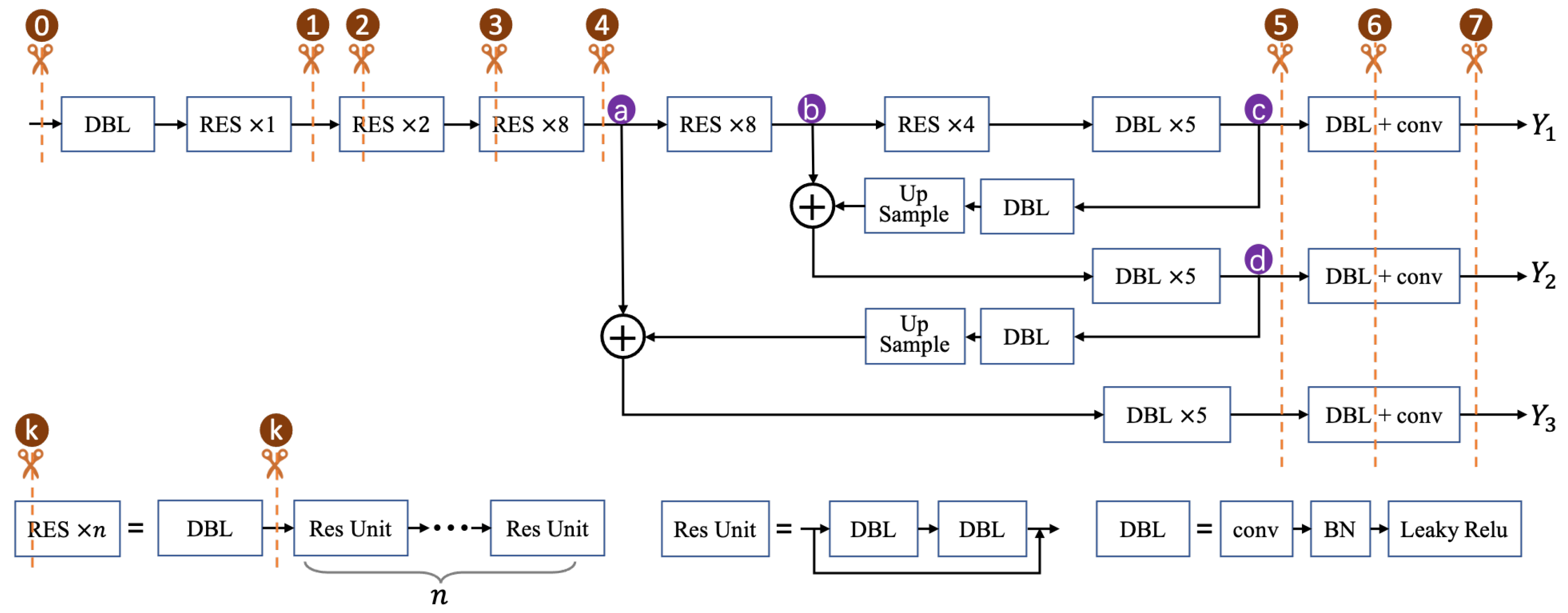
DNN model partitioning is a commonly adopted approach for accelerating DNN inference [6]. It splits DNN between two mid-layers and lets the local device conduct feed-forward inference of a few front layers and transmit small intermediate feature maps to the edge/cloud. The edge/cloud finishes the inference of the rest of the layers. With an appropriate split location, the whole video analytics system can achieve a small local workload and small bandwidth consumption at the same time. Take YOLOv3 [7] as an example; Figure 1 plots (a) the data size of the intermediate features and (b) time delay measured at different split locations. As the split location goes deeper, both data size and transmission time decrease, but the local inference time increases. Therefore, an appropriate split location should be selected for DNN partitioning to improve the overall system performance.
To trade off the local inference delay and intermediate feature transmission delay, there have been efforts to (1) search for the optimal split location under time-varying network conditions [8,9]; (2) distribute the inference workload to multiple computing nodes by splitting the DNN into multiple inference blocks [10]; and (3) encode intermediate features to smaller sizes for more efficient transmission [11,12]. These works; however, select the best split location by optimizing system performance only for the current frame, e.g., minimizing the transmission delay of the current frame, failing to consider the consequence of the current decision (e.g., a long waiting queue in the local device) to later frames.
In this paper, we propose DNN-Scissor, an edge-assisted DNN partitioning technique for cost-efficient, low-latency video analytics. Unlike existing works, DNN-Scissor optimizes long-term system performance using deep reinforcement learning. It learns a policy to dynamically select the optimal partition point from a pre-defined set of candidate locations by interacting with a real video analytics system and optimizing long-term rewards. This ensures the splitting decision for the current frame is also beneficial to later frames. The decision-making agent runs on the local device, while the edge server acts as a powerful computational resource to execute the offloaded portion of the inference task. Specifically, we jointly consider the workloads of the local device and the edge node, their bandwidth connection, and the video frame drop due to system overload. We design an Advantage Actor–Critic (A2C) -based algorithm for learning the optimal policy without complex system modeling. We implement the real-world system of DNN-Scissor and conduct policy learning and performance evaluation in a testbed to verify the effectiveness. The main contributions of the paper are summarized as follows:
  • Design an edge-assisted DNN model partitioning technique, DNN-Scissor, for cost-efficient, low-latency video analytics. DNN-Scissor optimizes long-term system performance including system workload, bandwidth consumption, and video frame drop.
  • Design a deep reinforcement learning-based algorithm to learn the optimal DNN splitting policy for each video frame to minimize the system cost over time.
  • Implement a real-world video analytics system testbed and conduct experiments to evaluate the performances.
The rest of the paper is as follows: Section 2 presents the related works, Section 3 illustrates the system design and workflows, Section 4 presents the problem formulation and learning algorithm, Section 5 evaluates the performances of our method, Section 6 details the system development and operational costs, Section 7 discusses the system scalability and adaptability, and Section 8 concludes this paper.

2. Literature Review

This section reviews the existing works that focus on DNN partition for accelerating DNN model execution and edge-assisted video analytics.

2.1. DNN Model Partition

The main challenge for DNN model partition is the trade-off between the local inference delay on the device and the transmission delay for offloading the intermediate features to the server for inference [6]. To determine the optimal partition point under varying network conditions, Neurosurgeon [8] designed a lightweight scheduler to automatically partition DNN computation between a mobile device and the data center at the granularity of neural network layers. Hu et al. [9] studied DNN inference acceleration with edge/cloud collaboration and proposed a Dynamic Adaptive DNN surgery (DADS) scheme that could partition DNN models between the edge and cloud based on dynamic network conditions. SPINN [13] proposed a distributed progressive inference engine that addresses the challenge of partitioning CNN inference across device–server setups. Dong et al. [14] designed an online algorithm based on Lyapunov optimization to optimally offload tasks by computation resource allocation and DNN partition. Tang et al. [15] considered a multi-user scenario and proposed a framework to address the multi-user DNN partition problem to minimize the delay among all users. PArtNNer [16] presented a characterization-free adaptive partitioning approach that uses runtime latency measurements to dynamically optimize DNN execution across edge/cloud platforms, achieving significant latency improvements over edge-only and cloud-only execution. APT-SAT [17] presented an adaptive framework for DNN partitioning and task offloading in satellite computing networks, employing reinforcement learning-based routing to optimize distributed DNN execution across multiple satellites while balancing workload distribution and resource utilization. Zhang et al. [18] presented a joint optimization framework combining DNN partitioning with task offloading, using attention mechanism-aided reinforcement learning (AMSAC), which dynamically allocates bandwidth resources based on task characteristics and employs a Soft Actor–Critic algorithm for adaptive layer-level partitioning to minimize inference latency in edge/cloud environments.
To tackle the limitation of the computing capacity of one single edge node, some works studied how to split the DNN model into multiple partitions and offload these partitions to multiple distributed edge nodes to complete inference collaboratively. Mohammed et al. [10] proposed an adaptive DNN partitioning scheme and designed a matching game-based distributed algorithm to offload the partitions to multiple powerful nodes. EdgeDI [19] proposed a framework for enabling model acceleration with distributed DNN inference by adaptively balancing the workload distribution among multiple devices under heterogeneous resource conditions. EdgeFlow [20] designed a new distributed inference mechanism for general Directed Acyclic Graph (DAG) structured DNN models. It first partitions the DNN model into independent units with a new progressive model partitioning algorithm and then assigns the independent units to different devices for parallel execution. CoEdge [21] proposed a distributed DNN computing system that orchestrates cooperative DNN inference over heterogeneous edge devices and designed a workload partitioning algorithm to decide partitioning policy in real time.
As transmitting the intermediate features to the edge may incur substantial delay, some works studied how to encode the intermediate features of DNN models to reduce offloading delay. JALAD [11] proposed an accuracy-aware approach for feature map compression to support DNN decoupling for edge/cloud execution. It adopts a normalization-based in-layer data compression approach by jointly considering compression rate and model accuracy. BottleNet++ [12] proposed an end-to-end deep learning architecture that consists of an encoder and a decoder for efficient feature compression and transmission. The encoder can perform adaptive coding under different channel conditions to keep robust while achieving graceful accuracy degradation with a noisy channel.
The main difference compared with the existing works is that we consider the dynamic workloads and the influence of the video frames on each other for model partition to minimize the cost over time.

2.2. Edge-Assisted Low-Latency Video Analytics

Many existing works have studied how to reduce bandwidth consumption and inference delays for video analytics [22]. To reduce the data size for video transmission, ACCMPEG [23] and CICO [24] adopted content-aware video encoding approaches to encoding different regions of a video frame into different qualities to reduce the video frame size by sacrificing some inference accuracy. ModelIO [25], Deepdecision [26], EdgeAdaptor [27], EdgeVision [28], EdgeCam [29], and A 2 [30] adopted DNN model adaptation to reduce inference delays. The video analytics system switches to inference with a smaller DNN model when the system workload is high. VideoStorm [31] and Chameleon [32] adopted frame rate tuning resolution resizing to reduce the transmitted video volume. CSVA [33] proposed a semantic-aware and complexity-driven video analytics approach by leveraging edge-cloud collaboration.
The adopted approaches in these works degrade the accuracy of the video analytics system due to lower video quality for encoding and downsizing and the choice of smaller DNN models for inference.

2.3. Conclusions of the Literature Review

The literature review reveals that while significant progress has been made in DNN partitioning, existing approaches exhibit key limitations. Competitor methods can be broadly categorized into two groups: (1) static- or heuristic-based partitioning and (2) myopic dynamic partitioning. Static approaches, such as pre-calculating a single optimal split point, are simple but inherently flawed as they cannot adapt to the highly dynamic nature of real-world network conditions and device workloads. Dynamic approaches improve upon this by making frame-by-frame decisions, but they are typically myopic or greedy. They optimize for the best immediate outcome for the current frame without considering the long-term consequences.
To overcome this limitation, this manuscript proposes a farsighted, learning-based approach to dynamic DNN partitioning. Our core research intent is to demonstrate that an agent can learn a sophisticated control policy that optimizes for a long-term, cumulative reward rather than an immediate one.

3. System Overview

In this section, we present the architecture and workflow of our edge-assisted video analytics system.

3.1. System Architecture

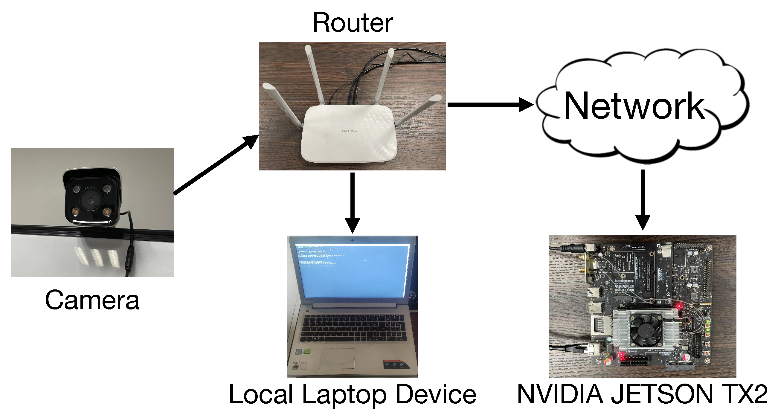
We illustrate the system architecture for edge-assisted video analytics in Figure 2. The system consists of three main components: camera, local device, and edge device. The local device reads video frames from the camera under a fixed interval (e.g., 100 ms). The DNN models for video analytics are deployed on both local and edge devices to perform inference. Our DNN-Scissor determines where to split the DNN model to distribute the DNN inference workload (i.e., feed-forward calculations) to the local device and the edge. The core of our method is the use of a small, efficient DRL network to learn the complex control policy for partitioning a much larger and more computationally intensive video analytics DNN (such as YOLOv3). Specifically, local device inferences from the original video frames and stops at the split location (e.g., vertical dash line with a scissor in Figure 2). The intermediate features are transmitted to the edge via the network. The edge continues to the rest of inference calculations to output video analytics results, e.g., locations of detected objects or image classes. The local device is usually with weak CPUs with fewer computational capabilities, while the edge is usually equipped with more powerful Graphics Processing Units (GPUs). We also use two queues on the local device; the local queue is to cache the pending inference tasks, and the offloading queue is to cache the intermediate frame features pending to be offloaded to the edge.

3.2. Workflow

DNN-Scissor performs edge-assisted video analytics with the following steps (see left to right in Figure 2):
  • The local device reads a video frame f t from the camera at a specified reading interval and pre-processes (e.g., resizes) the frame.
  • The DNN-Scissor agent, running on the local device, observes the current system state such as the length of local queues and current network bandwidth, and makes a decision on where to split the DNN for frame f t .
  • Together with this splitting decision, frame f t is then put into the local queue waiting for local inference.
  • DNN-Scissor monitors the waiting time of f t . Once the waiting time exceeds a time-out threshold, f t will be dropped directly.
  • The local device calculates the DNN layer by layer for f t until the split location.
  • The intermediate features from the split location are then put into the offloading queue for transmitting to the edge. The features will also be dropped once the waiting time exceeds the time-out threshold.
  • The edge continues the feed-forward calculations for the rest of the DNN layers and outputs analysis results.

4. Methodology

In this section, we first introduce preliminary concepts of the system and then formulate splitting DNN as a reinforcement learning problem; we finally present an A2C-based algorithm to learn the optimal splitting policy.
DNN-Scissor aims to select the best location to split DNN models so that the local device can have a smaller feed-forward inference workload and transmit smaller sizes of intermediate features to the edge, letting the more powerful edge finish the inference on the rest of the DNN layers. The split location should be able to optimize system performances such as minimizing total time delay, network bandwidth consumption, and drop rate.

4.1. Preliminaries

Here, we introduce concepts in our edge-assisted video analytics system.
DNN partitioning is to separate the feed-forward calculations of a DNN model into two stages. The first stage computes from the input layer to the layer just before the split location on the local device. The second stage takes the intermediate features as the input and starts to compute from the split location to the output layer on the edge device.
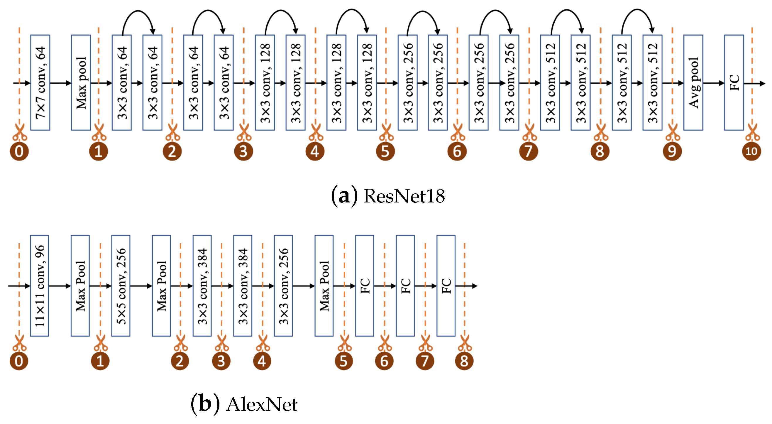
Candidate split locations: A simple DNN structure, such as AlexNet [34], stacks convolution or fully connected layers one by one. Splitting between any two layers results in only one 3D matrix of the feature map and clearly separates feed-forward calculations into two stages for local inference and edge inference. However, more complicated DNNs may have multiple branches, such as YOLOv3 [7] (see Figure 3), for fusing features at different scales or outputting multiple results. There are also branches (e.g., locations c and d in Figure 3) that forward deeper features to fuse into earlier layers. Splitting on one branch may not be able to separate feed-forward calculations into two stages clearly. For example, in Figure 3, if we split on c only, we still need to determine whether to calculate Y 2 and Y 3 branches on local or edge. Therefore, we take the DNN as a DAG, in which each node is a layer, and edges are links between layers. A candidate split location is a graph cut of the information flow from the input layer to the output layer. The flow cut must ensure that the local device does not need deeper features calculated in edges. By this principle, we select a set of candidate split locations for YOLOv3, illustrated by the vertical dashed lines with circled numbers in Figure 3. Locations 1 to 4 can split the network layers into two sets with one intermediate 3D feature map. Each of the 5 to 6 locations splits the three branches in parallel, resulting in three intermediate 3D feature maps. This set of candidate locations is pre-defined and remains fixed for a given DNN model. The core task of our DNN-Scissor agent is to dynamically select the most appropriate location from this fixed set for each incoming video frame based on the real-time system state.
Data amount is the total data size of all the intermediate features in bytes to be transmitted to the edge.
Total delay of a frame is the total time from reading the frame from camera to outputting inference results on edge. It includes the waiting time at the local queue, local inference time, waiting time at the offloading queue, network transmission time, and edge inference time. The smaller the total delay, the more efficient the system.

4.2. DNN Partitioning as a Dynamic Graph Cut Problem

The task of splitting a DNN can be formally modeled as a graph partitioning problem. A DNN is a DAG, denoted as G = ( V , E ) , where V is the set of layers (vertices) and E represents the data flow dependencies between them (edges). A DNN partition, as defined in our work, is a cut that partitions the vertex set V into two disjoint subsets: V l o c a l , representing the layers executed on the local device, and V e d g e , representing the layers offloaded to the edge server. The set of edges that connect a vertex in V l o c a l to one in V e d g e represents the data that must be transmitted over the network.
This problem is related to classic graph partitioning challenges, most notably the Minimum Cut (Min-Cut) problem. If the sole objective were to minimize the amount of data transferred, the task would be to find a cut where the size of the edge-set crossing the partition is minimized. However, our problem introduces two key complexities that distinguish it from standard graph cut formulations:
  • State-Dependent Costs: The true cost or expense of a partition is not a static property of the graph. It is dynamic and state-dependent. The data transfer cost (latency) depends on the real-time network bandwidth, and the computational cost (latency) depends on the current workloads of the local and edge devices. Classic graph algorithms typically operate on graphs with fixed, pre-defined weights.
  • Long-Term Sequential Objective: We do not seek a single, static optimal partition. Instead, the goal is to learn a dynamic policy that selects the best partition for each incoming video frame to maximize a cumulative, long-term reward. This objective requires a farsighted approach that considers the future consequences of a current action (e.g., preventing future queue build-up), which is a characteristic of sequential decision problems.
Given these complexities, standard graph partitioning algorithms are not a direct fit. Therefore, we formulate this dynamic, state-aware partitioning task as a sequential decision-making problem and leverage DRL to learn an optimal control policy.

4.3. Deep Reinforcement Learning Modeling

Dynamically splitting DNN layers to adapt to the changing network conditions can be modeled as a reinforcement learning problem. We define an agent to interact with the communication network environment. As illustrated in Figure 4, when the agent reads a video frame from the camera, it observes the network statuses, selects a layer to split DNN, distributes the inference workload to the local and edge devices separately, and receives a reward after the inference completes. In the following, we present detailed definitions of state, action and reward.
The state at time t, denoted by s t , includes the workloads, network bandwidth, time delay, and the amount of data to be transmitted. Specifically, we define the workloads by the number of frames l t in the local queue on the local device and the number of intermediate feature maps c t in the offloading queue to the edge. These two state factors can be easily observed in the system. However, network bandwidth, time delay, and the data amount of frame f t cannot be observed until the splitting action is executed and f t is computed. Therefore, we estimate them by the current observations at time t of previous frames. For network bandwidth, we estimate by the observed bandwidth when transmitting current intermediate data from the local device to the edge. The transmitted data could be the features of a previous frame. We denote the bandwidth estimation as b ^ t .
For time delay, we estimate from the previous frames in the local queue and features in the offloading queue. For each previous frame i, we already know its splitting action (i.e., locations to split), so it is easy to estimate its local inference time τ ^ local i and edge inference time τ ^ edge i , t l t i < t . For each intermediate feature data in offloading queue j ( 1 j < c t ), the edge inference time τ ^ edge j can also be easily estimated. So we estimate the total delay of f t by the sum of all the local and edge inference time estimations of all waiting frames and the edge inference time of all waiting feature data; i.e.,
τ ^ t = t l t k < t ( τ ^ local k + τ ^ edge k ) + 1 j < c t τ ^ edge j .
Note that this is an underestimation because the actual inference time of f t and the transmission time of all the waiting frames are not included. However, τ ^ t can still be a good observation in the state as it already contains the time details of system workloads. Knowing how long to wait for inference can help generate actions to optimize long-term system performance.
For the data amount to be transmitted, we sum up the amounts of all the intermediate data to be transmitted of all the waiting frames in the local queue, denoted by o i , and feature data in the offloading queue, denoted by o j , as the data amount observation in the state, namely,
o ^ t = t l t k < t o i + 1 j < c t o j .
Note that the data amount of feature map for frame f t is unknown and not included. Knowing how much data to be transmitted in the near future at time t can also help improve long-term system performance.
Overall, the state for frame f t is summarized as a vector of the observations and estimations; i.e.,
s t = [ l t , c t , b ^ t , τ ^ t , o ^ t ] .
The action of the agent is to decide which layers to split and distribute the DNN inference workload of a frame to local and edge devices. This means that the local inference on the device will be stopped at the spitting layer, transmitting the intermediate features to the edge, and the edge device will continue to compute the rest of the layers. In most deep neural networks, deeper layers generate more dense features with a smaller data size, leading to less bandwidth consumption and a smaller workload on the edge but a larger workload on the local device. Given that local devices usually have less computational power than edge devices, splitting on a shallower layer helps reduce workload on the local device but may generate a larger intermediate feature map and thereby high bandwidth consumption. Therefore, a good action should be able to balance between local workload, bandwidth consumption, and edge workload in a dynamic network environment.
The reward of an action for frame f t evaluates the system performance in total time delay τ t and the amount of transmitted data o t . The less time delay and fewer data for a frame, the more reward. We consider the total time delay τ t to include waiting time in the local queue, local inference time, waiting time in offloading queue, transmission time, and edge inference time. The total delay can be directly obtained after frame f t is analyzed. We introduce a penalty weight w, w 0 , to balance the importance between data transmission and time delays in measuring system performance; i.e., the reward of successful inference for f t is w × o t τ t . Setting a higher w encourages smaller data transmission but may cause a longer time delay.
Note that we set dropping frames when they waited too long in the local queue, i.e., more than T seconds, for the sake of system efficiency. In this case, we penalize with a large fixed positive value F for those frames. In summary, the reward is defined as
r t ( s t , a t ) = w × o t τ t , m t T F , m t > T ,
where m t is the waiting time of frame f t in the local or offloading queue; we set the waiting time threshold T as 2 s for segmenting YOLOv3 and 0.5 s for ResNet18 [35] and AlexNet [34]. We also set the drop penalty F as 10 in the experiments.

4.4. Splitting Policy Learning Algorithm

DNN-Scissor adopts the A2C network to learn the policy of selecting splitting locations for DNNs. As illustrated in Figure 5, we define actor network π ( a t | s t , θ ) to generate the probability of splitting on each candidate location, with observed state s t and a set of network parameters θ . The critic network v ( s t , ϕ ) estimates the value for state s t with a set of parameters ϕ . The actor network updates θ by the loss function
L ( θ ) = t B ln ( π ( a t | s t , θ ) ) δ t .
where δ t is the TD error, i.e., δ t = r t + γ v ( s t + 1 , ϕ ) v ( s t , ϕ ) , with the discount factor γ . B is the set of sampled transitions from the replay buffer. The critic network updates ϕ by the MSE loss function,
L ( ϕ ) = 1 | B | t B ( v ( s t , ϕ ) G t ) 2 ,
where G t denotes the TD target, i.e., G t = r t + γ v ( s t + 1 , ϕ ) .
Algorithm 1 depicts the general procedures of training DNN-Scissor. We define an episode as a time step of reading a coming frame and initialize the actor network θ , critic network ϕ , and empty replay buffer M. For each new coming frame f t , DNN-Scissor observes lengths of the local queue and the offloading queue, the current network bandwidth, and estimates the total time delay and the total amount of data to be transmitted (Lines 3 to 6). With this state information, the algorithm directly samples an action (i.e., a split location) from the actor network θ , and then pushes the frame f t into the local queue for further inference. We update state s for the next coming frame. Meanwhile, we monitor the waiting time m t of frame f t in the local queue. Once m t exceeds the threshold T, f t will be dropped, and we will obtain penalty reward F (Lines 10 to 12). Otherwise, we execute the action, i.e., split the DNN on the location a, compute the front layers on the local device, transmit the intermediate features to the edge, and infer the rest layers on the edge. The total inference time τ t and the data size of intermediate features o t are recorded. We then receive a reward of w × o t τ t (Lines 14 to 15). The transition [ s , a , r , s ] is stored in the replay buffer M. Both actor network θ and critic network ϕ update every five time steps (frames) with the set of sampled transitions B from replay buffer M (Lines 18 to 22), using gradient descend with step sizes α θ and α ϕ separately. The algorithm terminates until rewards converge.
Algorithm 1 DNN splitting policy learning with A2C
Input: Initialized actor θ and critic ϕ , empty replay buffer M
  1: while rewards not converged do
  2:     Read a frame f t from camera
  3:     Obtain lengths of local queue and offloading queue
  4:     Obtain current network bandwidth
  5:     Estimate time delay and data amount by Equations (1) and (2)
  6:     Get state s by Equation (3)
  7:     Sample split location a π ( · | s , θ )
  8:     Put f t into the local queue
  9:     Update state s
10:     if  m t > T  then
11:         Drop f t
12:         Get reward r = F
13:     else
14:         Split the DNN at a and inference f t
15:         Get reward r = w × o t τ t
16:     end if
17:     Store [ s , a , r , s ] to M
18:     if time to update then
19:         sample set of transitions B from M
20:         Update actor by θ : = θ + α θ L ( θ )
21:         Update critic by ϕ : = ϕ + α ϕ L ( ϕ )
22:     end if
23: end while

4.5. Algorithmic Complexity

At inference time, the partitioning decision for an incoming frame is made by performing a single forward pass through the agent’s policy network. This network is a small, two-layer, fully connected neural network. The computational complexity of this forward pass only depends on the size of the state vector and the dimensions of the network’s hidden layers. The complexity is constant and independent of the size or depth of the target analytics DNN being partitioned. Therefore, the complexity of the decision-making step is O ( 1 ) with respect to the number of layers in the target model.

5. Results

In this section, we present experimental settings and evaluate the performance of our proposed method with baselines.

5.1. Experimental Settings

5.1.1. Experimental Environment

We developed a real system as the testbed (see Figure 6) for experiments. The testbed uses an industrial camera DAHUA HFW2433M-A-IL (Dahua Technology Co., Ltd., Hangzhou, China) to capture videos; it is connected to the local laptop Lenovo Ideapad with a CORE-i5 CPU and 8 G memory by a router. The local device reads the video frames at a certain reading rate with the Real-Time Streaming Protocol (RTSP) streaming protocol. The local device sends frames or their compressed features to an edge device NVIDIA JETSON TX2 (NVIDIA Corporation, Santa Clara, CA, USA, https://developer.NVIDIA.com/embedded/jetson-tx2, accessed on 15 May 2025), with an NVIDIA Pascal GPU and 8 G memory. All the communication among these devices is by the router, and the router connects with the edge node through a congested campus network. We also evaluate the performances of our method under different fixed bandwidth connections. Both local and edge devices use the Linux operating system with version Ubuntu18.04. We developed the whole system with Python 3.13 and PyTorch 2.3, and implemented our DNN-Scissor on the local device and the edge node.

5.1.2. Hyperparameters and Settings

In DNN-Scissor, both actor and critic networks use a fully connected neural network with two layers, each with 16 neurons. The activation functions of the first and the last layers are ReLu and Softmax separately. The batch size is 5, the reward discount is 0.95, and the learning rate is 0.001.
We test DNN-Scissor and other baseline methods on three DNN segmentation tasks, i.e., segment YOLOv3 for downstream application of object detection, and ResNet18 and AlexNet image classification. All three DNNs are pre-trained and downloaded from PyTorch Hub (https://pytorch.org/hub/, accessed on 15 May 2025). Table 1 lists the basic information about the three DNNs including trained network file size and number of parameters. We also run each DNN on our local device and edge device independently and report the inference time in Table 1. YOLOv3 takes a much longer time (4.347 s) on the local devices than others because of its high complexity, but the three DNNs have a similar inference time on the more powerful edge with a GPU.
We also select different sets of candidate split locations for each DNN, from which our DNN-Scissor aims to select the optimal one to split. Figure 3 and Figure 7 show exact split locations on YOLOv3, ResNet18, and AlexNet, respectively. Unlike YOLOv3 (Figure 3), which has split locations on network branches, the candidate split locations of ResNet18 (Figure 7a) are between every residual block, so each location can break the network into two parts, resulting in one block of intermediate feature matrices. AlexNet (Figure 7b) is in a typical chain structure, so the candidate split locations are between every convolution block and every fully connected (FC) layer.
By default, the reading rates of YOLOv3, ResNet18, and AlexNet are 1000 ms, 150 ms, and 150 ms per frame. To avoid overload, we also drop frames when the number of frames waiting at the local queue or offloading queue exceeds a threshold. We set the threshold as 2 s for YOLOv3 and 0.5 s for both ResNet18 and AlexNet.

5.1.3. DRL Agent Training Setup

Episode Definition: Our system processes a continuous stream of video frames. To train the DRL agent, we define an episode as the processing of a fixed sequence of 1000 consecutive video frames. At the end of each episode, the system’s state (e.g., queues) is reset, but the learned policy network weights are carried over to the next episode.
Convergence Criteria: The training process was continued for a maximum of 500 episodes for each model. We determined convergence by monitoring the moving average of the total reward per episode. Training was considered to have converged when the average episodic reward over a sliding window of the last 50 episodes no longer showed a statistically significant improvement and stabilized around a consistent value.
Variance and Reproducibility: The performance of DRL agents can be sensitive to the initial random seed. To ensure that our results are robust and not an artifact of a single lucky run, all reported evaluation metrics and reward curves are the average of five independent training runs, each initialized with a different random seed. The final policy used for the evaluation is the one corresponding to the run with the median final performance.

5.1.4. Data Set

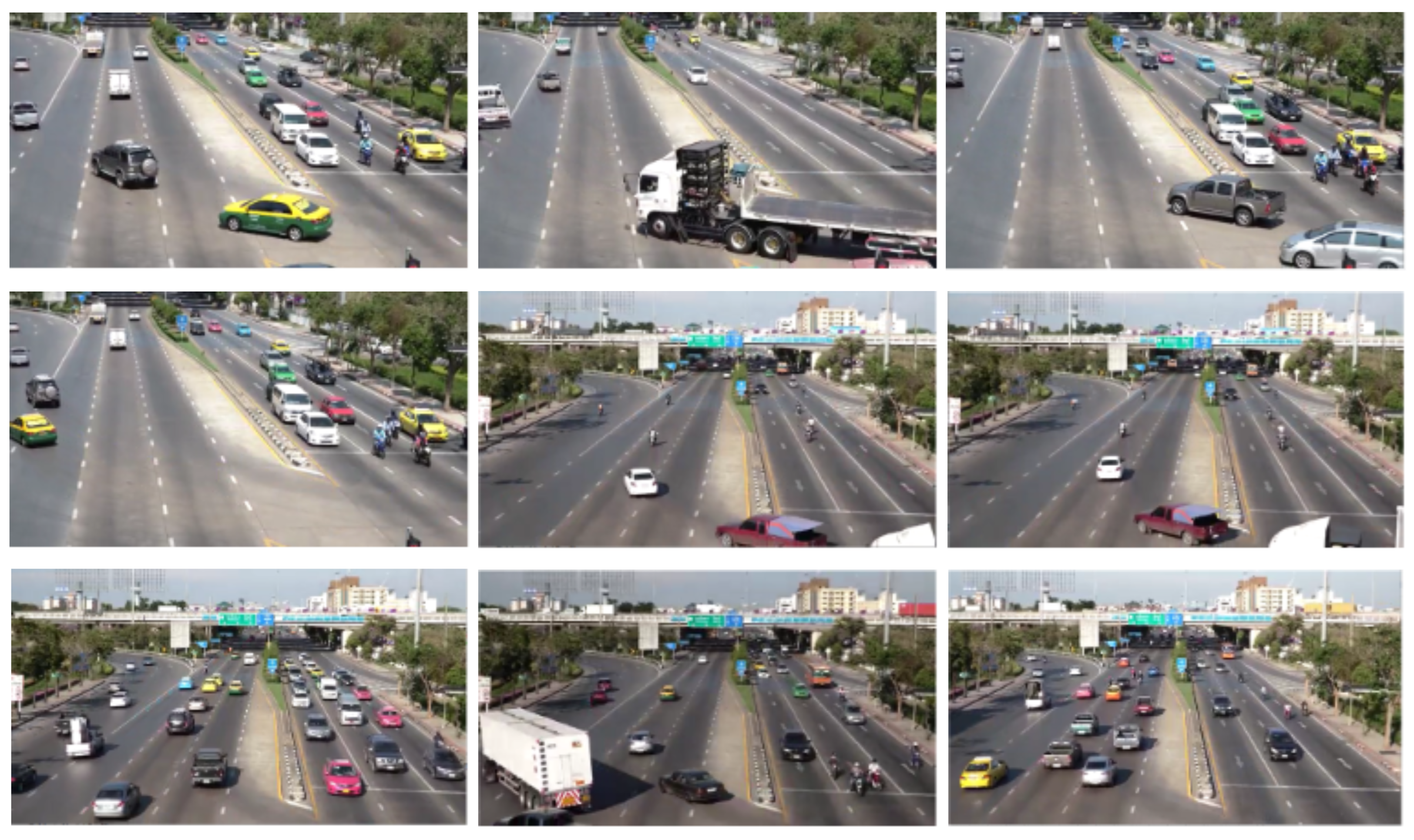
Instead of using a real-time video camera equipped in our local campus that captures a relatively simple scene with a few vision objects, we test with open-traffic video camera data (https://github.com/KuntaiDu/dds, accessed on 15 May 2025), which is much more complex with many more objects (see Figure 8). The whole video data set contains a total of 5146 frames in a high resolution of 1080 P.

5.1.5. Human-in-the-Loop Configuration

While our system automates the dynamic partitioning decision for each frame, several key architectural choices and parameters are configured by a human designer or operator. Here, we explicitly detail those human-in-the-loop decisions to ensure transparency and reproducibility. The following aspects of the DNN-Scissor framework are set by humans:
  • Choice of Analytics DNN: The specific DNN model used for the vision task (e.g., YOLOv3, ResNet18) is a manual design choice based on the application’s requirements for accuracy and performance.
  • Selection of Candidate Split Points: The set of potential layers where a partition can occur is pre-defined by a human. This selection is guided by the DNN’s architecture, targeting layers where the output feature maps form a logical bottleneck or transition point. The DRL agent’s role is to automatically select the best option from this pre-defined set.
  • DRL Agent Architecture and Hyperparameters: The structure of the DRL agent’s neural networks (e.g., number of layers and neurons in the actor and critic networks) is a manual design choice. Additionally, key training hyperparameters are set by a human, including the learning rate, the reward discount factor ( γ ), the trade-off weight (w) in the reward function, and the penalty (F) for dropping a frame.
  • System Operational Parameters: The operational settings for the video analytics pipeline are configured manually. This includes the video frame reading rate (e.g., 1000 ms per frame for YOLOv3) and the time-out threshold (T) that determines when a waiting frame is dropped. These are typically set based on the specific application’s latency requirements and the available hardware resources.

5.1.6. Baselines

We compare our DNN-Scissor with the following methods:
  • Device Only: This method runs deep neural networks at the local device.
  • Edge Only [36]: This method receives the original video frames and runs deep neural networks at the edge.
  • Semi-Fixed [2]: This method either splits DNNs at a fixed layer (not the first one) or directly processes video frames at the edge when the number of waiting frames exceeds a threshold. We set the fifth layer to split for each DNN partition task, and the threshold is set to 10.
  • Greedy [8]: This method selects the best split location that maximizes the current system performance measured by the transmitted data amount and processing delay for each video frame independently. The overall delay for this approach is estimated by predicting the queuing delay and the transmission delay under an estimated bandwidth.

5.1.7. Metrics

We evaluate system performance with the following metrics:
  • Transmitted Data Amount, i.e., o t , is the data size to be transmitted from the local device to the edge per video frame, measured by bytes.
  • Total Delay, i.e., τ t , is the total time delay per video frame, including the local inference and edge inference times, waiting times in queues, and transmission time.
  • Local Delay is the local inference time per frame.
  • Edge Delay is the edge inference time per frame.
  • Drop Rate is the percentage of frames dropped because of long waiting times in either local queue or offloading queue. All the compared methods have the same time threshold dropping frames.
  • System Cost is the average magnitude of reward per frame. It is either the weighted sum of the transmitted data amount plus the total delay, i.e., w × o t + τ t , when a frame got computed, or 10 when a drop is dropped. The trade-off weight w is set to 1 by default.
It is noteworthy that the purpose of splitting DNNs is to improve the transmission efficiency of the communication network; since we did not trade DNN accuracy for inference efficiency, the performance of the DNN itself, such as classification accuracy, should be the same no matter how the DNN is split. We have verified this to ensure the correctness of all the experiments but excluded DNN accuracy from our evaluation metrics.

5.2. Experimental Results

5.2.1. Comparison Results

We compare DNN-Scissor with the baseline methods in terms of the average transmitted data amount per frame, total processing delay per frame, and drop rate. Figure 9 plots the results of the comparison. We can observe that DNN-Scissor achieves the shortest total delay and the minimum system cost among all the methods. This demonstrates the effectiveness of DNN-Scissor in improving communication efficiency for video analytics.
We also observe that (1) Edge Only transmits the most amount of data, as it directly sends the pre-processed frame images to the edge. Note that YOLOv3 uses a different pre-processing technique for object detection; the data size is larger than that of ResNet18 and AlexNet for image classification. The edge processes the frame images with a relatively powerful GPU, so the total delay is relatively small and with a low drop rate. (2) Local Only inference on the local device has less computational power. Even though it transmits a few data points (just object detection or classification results) to the edge, it suffers the highest total delay and drop rate due to the incapability of the local device. (3) Compared to Edge Only and Local Only, Semi-Fixed trades the amount of data with total delay by forwarding the frame images directly to the edge when frames waiting for the local device exceed a threshold. So it has a less amount of data than Edge Only and less delay than Local Only, but it splits DNN at a fixed layer, failing to adapt to dynamic network conditions, thus leading to a higher system cost than our DNN-Scissor. (4) Greedy makes a worse trade-off between the data amount and time delay compared to Semi-Fixed. Although it searches for the best split location based on the prediction of the networking environment, the prediction accuracy affects the choice of split location. In contrast, our DNN-Scissor achieves the best performance by searching for the best split layer not only based on the current networking observation but also based on the estimation of future dynamic networking environments by A2C networks. It puts more layers on the local device to reduce data size to be transmitted when the network conditions are poor or transmits more data to the edge for more efficient inference under good network conditions.
The results in Table 2 summarize the performance gains of our approach. For the complex YOLOv3 model, DNN-Scissor reduces the total end-to-end delay by 86% compared to a purely local execution and by 83% compared to a myopic greedy strategy. This efficiency translates to a 67% reduction in overall system cost against the same greedy baseline. Most critically, it enhances stability by reducing the frame drop rate by 56% compared to the overloaded local-only method, ensuring a more reliable pipeline.

5.2.2. Verification of Inference Accuracy

A foundational premise of our work is that model partitioning is a mathematically lossless operation that does not affect the final inference accuracy. The feed-forward computation is merely distributed across two devices, but the sequence of operations and the model weights remain identical.
To formally verify this claim, we ran a sample image through the AlexNet model under multiple partitioning configurations and compared the final output logits. As shown in Table 3, the top one predicted class and its corresponding logit value are numerically identical across all split points, confirming that our partitioning framework preserves the model’s accuracy. This holds true for all models used in our evaluation.

5.2.3. Effects of Network Bandwidth

To study how the bandwidth affects the performance of all the methods, we set various fixed bandwidths, i.e., 1 MBs, 5 MBs, and 10 MBs, in our testbed and compared metrics between methods. Since ResNet18 and AlexNet are smaller and less complex, we conducted experiments only for the larger YOLOv3. Figure 10 plots the transmitted data amount, total delay, drop rate, and system cost for each method under the three bandwidth settings. We can easily observe that all the metric values decrease with the increase in bandwidth in each method, except that Edge Only, Local Only and Semi-Fixed have constant data amounts because the three methods transmit data at fixed locations. This demonstrates that with better network conditions, the video analytics system performs better in each splitting method. Furthermore, our DNN-Scissor achieves the shortest total delay and zero drop rate, and DNN-Scissor achieves the lowest system cost.

5.2.4. Sensitivity Analysis of the Reward Trade-Off Weight (w)

The trade-off weight, w, in our reward function (Equation (4)) is a critical hyperparameter that governs the agent’s learned behavior. It allows a system operator to define the relative importance of minimizing transmitted data versus minimizing total latency. To understand the impact of this parameter and to justify our choice for the main experiments, we conduct a sensitivity analysis with different values of w.
We set trade-off weight w to trade off between the transmitted data amount and the total latency (see Equation (4)). To evaluate how the weight affects the performance of DNN-Scissor, we compare the data amount, total delay, edge delay, and local delay with different weights from 0 to 2 for segmentation tasks on YOLOv3, ResNet18, and AlexNet. Figure 11 plots the comparison results. We can observe that with the increase in data weight, the average data amount to be transmitted decreases (Figure 11a), but the total delay increases (Figure 11b) for each DNN segmentation. This indicates that by tuning the weight, DNN-Scissor can flexibly trade off between the data amount and the latency.
We also compare the delays on the edge and local devices (Figure 11c,d) with varying trade-off weights. For YOLOv3, the most delays happen on the edge as the local device is unable to compute such a complex DNN, leading to the largest transmitted data amount (Figure 11a). This indicates that our DNN-Scissor selected early split layers of YOLOv3 in most cases. In contrast, the relatively small DNNs ResNet18 and AlexNet have much shorter delays on edge, demonstrating that DNN-Scissor selects deeper layers to split and puts most calculations on the local device, leading to much smaller data transmitted. Overall, DNN-Scissor flexibly selects split layers to trade off the inference workload between the edge and local device to reduce both data amount and total delay. In addition, we found that the waiting times in both queues can be negligible in DNN-Scissor, demonstrating the effectiveness of the penalization F.
This analysis demonstrates that the choice of w is not arbitrary but a deliberate configuration choice to tune the system’s policy for specific deployment goals (e.g., for a metered connection versus a low-latency application). For our main experiments, we chose w = 1.0 as a balanced setting that gives comparable importance to both data and latency costs.

5.2.5. Analysis of Latency Components and System Adaptability

To provide deeper insights into the system’s behavior, we present an empirical breakdown of the latency components and discusses how the agent’s policy leads to real-time adaptability in dynamic environments.
The DRL agent’s primary task is to intelligently trade off the different sources of latency—local computation, network transmission, and edge computation; while our sensitivity analysis in Figure 11 shows the effect of the trade-off weight w on the computation components, Table 4 provides a more direct empirical breakdown, including the transmission cost, for two distinct scenarios that the agent learns to navigate.
The data in Table 4 is derived from our experiments and illustrates the two opposing strategies our agent learns. When network conditions are favorable (emulated by a policy trained with a low w), the agent selects a shallow split point. This minimizes demanding local computation, offloading the majority of the work (49% of the latency) to the edge, accepting a moderate transmission cost (18%). Conversely, when the network is poor (emulated by a policy trained with a high w), the agent learns to choose a deep split point. This strategy dramatically increases local computation time but crucially reduces the transmission cost to a negligible level (4%), avoiding a network bottleneck.
The results above demonstrate that the agent can learn fundamentally different, specialized policies. The “real-time adaptability” of a single, trained agent stems from its ability to switch between these strategies dynamically based on the real-time state.
Our agent is designed to be state-aware. If an agent trained with a balanced policy ( w = 1 ) encounters a sudden drop in network bandwidth, the state variables for bandwidth ( b ^ t ) and queue length ( c t ) will change. The agent’s learned policy will then map this new state to an action that favors a deeper split point, mirroring the behavior shown in the “Low Bandwidth” row of Table 4. When the network recovers, the state changes again, and the agent will revert to selecting shallower split points.

5.2.6. Effects of Frame Reading Rate

The reading rate of video frames also affects system performance. A smaller reading rate (time interval between frames) leads to a heavier workload and thus longer delays and an even higher drop rate. Therefore, we vary the reading rate to evaluate how our algorithm performs with various workloads. Table 5 summarizes three settings of the reading rate for each DNN segmentation task. As YOLOv3 is much more complex than the other two DNNs, requiring much larger computation resources, we set its reading rate to vary from 800 ms to 1200 ms, while that of ResNet18 and AlexNet is set to vary from 100 ms to 200 ms.
Figure 12 plots the (a) data amount, (b) total delay, (c) drop rate, and (d) system cost of our DNN-Scissor on segmenting the three DNNs in different levels of reading rates. It can be observed that with the increasing reading rate, the total delay, drop rate, and system cost decreases (Figure 12b–d), but the amount of transmitted data slightly increases. This is because the larger reading rate indicates smaller workloads so that both the local device and edge can compute faster and a smaller number of frames will be in waiting queues. With less workload, DNN-Scissor tends to choose more front layers to split and more layers for inference on edge, leading to large data amounts to be transmitted. However, the overall system cost decreases. Also, we set the drop threshold as 2 for YOLOv3 and 0.5 for both ResNet18 and AlexNet due to the significant scale difference between YOLOv3 and the other two. So the drop rate of YOLOv3 is quite small. However, for the same drop threshold, ResNet18 has a much higher drop rate because ResNet18 is much more complex than AlexNet.

5.2.7. Reward Convergence

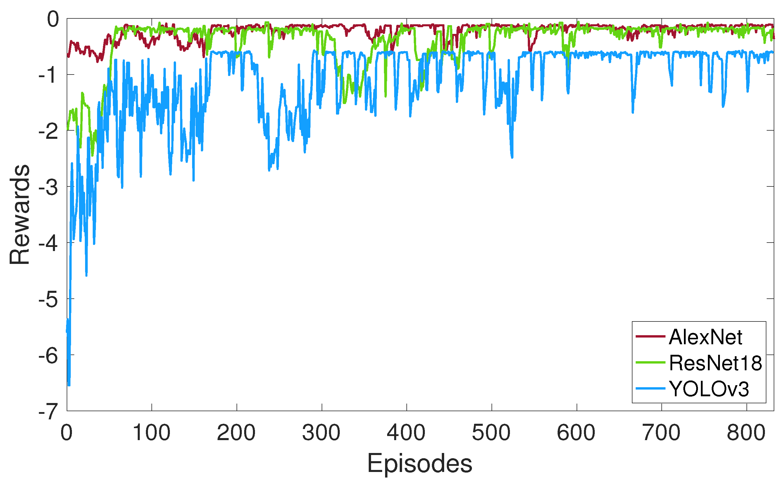
We evaluate the performance of training our DNN-Scissor by reward convergence. Figure 13 plots the rewards when training DNN-Scissor for segmenting three neural networks: YOLOv3, ResNet18, and AlexNet. All the rewards in the three training processes converge after a few hundred episodes. The reward magnitude of the small networks, i.e., ResNet18 and AlexNet, are smaller than that of the large network YOLOv3. This is because large neural networks need a much longer time for inference than small neural networks.

5.2.8. Robustness to Dynamic Conditions

A critical requirement for any real-world video analytics system is robustness to dynamic conditions such as unstable network bandwidth and bursty video workloads. The DRL-based approach of DNN-Scissor is fundamentally designed for dynamic environments. The agent’s policy takes the current system state as input. This state includes the lengths of the local and offloading queues and the estimated network bandwidth.
In the case of an unstable or degraded network, the bandwidth estimate would decrease, and the offloading queue would begin to grow. The agent’s learned policy would react to this change in state by selecting a deeper partition point, thereby reducing the size of the intermediate features to alleviate network pressure. In the case of a bursty workload, the local queue would rapidly increase. The agent would react to this by selecting a shallower partition point, offloading more computation to the powerful edge server to clear the local backlog more quickly, provided the network can support it. This state-aware, adaptive decision-making process allows the system to gracefully handle real-world instabilities.
Our primary experiments are conducted over a live, shared campus network, which is subject to unpredictable traffic and bandwidth fluctuations. The superior performance of DNN-Scissor in this environment is direct evidence of its robustness. As shown in Figure 9c, the baseline methods (especially Local Only and Greedy) exhibit high frame drop rates, indicating their inability to cope with system dynamics. In contrast, DNN-Scissor maintains a low drop rate, demonstrating that its adaptive policy successfully navigates these real-world instabilities to maintain a stable processing pipeline.

5.3. Computational Cost Analysis

This section provides a thorough accounting of the computational expenses at each stage of the DNN-Scissor pipeline during runtime. The costs are primarily discussed in terms of latency, which is the critical metric for low-latency video analytics. The pipeline is divided into three main stages: pre-processing, processing, and post-processing.

5.3.1. Pre-Processing Expenses

This stage prepares a raw video frame for inference. All pre-processing tasks are executed on the local device’s CPU.
  • Tasks: The pipeline begins by capturing a frame from the video stream. The frame is then decoded and resized to the required input dimensions of the target DNN (e.g., 416 × 416 for YOLOv3). Finally, pixel values are normalized.
  • Expenses: These are standard, efficient computer vision operations. On a typical CPU like the one in our testbed, the combined latency for these tasks is minimal, generally in the range of 5–15 ms per frame. The computational cost is low and predictable.

5.3.2. Processing Expenses

This is the core stage where the DNN inference is performed and constitutes the vast majority of the system’s cost. The expenses are distributed across the local device, the network, and the edge server.
  • 1. Partition Decision:
     
    Location: Local device (CPU).
     
    Task: The DRL agent performs a forward pass through its policy network to select the optimal split point.
     
    Expense: As established, the complexity is O(1) with respect to the analytic DNN’s size. This is an extremely fast operation, incurring a latency of only 1–2 ms.
  • 2. Local Inference:
     
    Location: Local device (CPU).
     
    Task: The local device executes the initial layers of the DNN up to the chosen split point.
     
    Expense: This is a major variable cost. The latency depends directly on the partition decision. A shallow split (fewer layers processed locally) results in low latency, while a deep split results in high latency. This cost can range from a few milliseconds to several seconds, as shown in our experimental results.
  • 3. Data Transmission:
     
    Location: Network.
     
    Task: The intermediate feature map is serialized and transmitted from the local device to the edge server.
     
    Expense: The cost is network latency, which depends on the size of the feature map (determined by the split point) and the available network bandwidth. This cost is also highly variable and is a key factor in the DRL agent’s decision-making.
  • 4. Edge Inference:
     
    Location: Edge server (GPU).
     
    Task: The edge server executes the remaining layers of the DNN.
     
    Expense: Due to the powerful GPU, the per-layer processing time is significantly lower than on the local CPU. The total latency on the edge depends on the number of layers it needs to process (the inverse of the local inference cost).

5.3.3. Post-Processing Expenses

This stage involves interpreting the final output of the DNN to generate a human-readable result. All post-processing is performed on the edge server.
  • Tasks: For an object detection model like YOLOv3, this includes applying non-maximum suppression (NMS) to filter redundant bounding boxes and decoding the final tensor into class labels and coordinates. For a classification model, this is a simple operation to find the class with the highest probability score.
  • Expenses: These operations are computationally inexpensive compared to the DNN inference itself. On the edge server, the post-processing latency is typically very low, in the range of 2–5 ms.

6. System Development and Operational Costs

This section details the functioning expenses of the DNN-Scissor system, broken down by the key stages of development. The costs are estimated in terms of the required skills and the number of person-hours, providing a transparent overview of the human capital investment.

6.1. Data Collection

  • Skills Needed: Graduate Researcher with basic knowledge of computer vision datasets.
  • Task Description: Our experiments utilize a publicly available traffic video dataset. This stage involved searching for suitable datasets, selecting one that met our criteria for complexity and resolution, and downloading the video files.
  • Estimated Person-Hours: 4–6 h.

6.2. Data Cleaning

  • Skills Needed: Graduate Researcher.
  • Task Description: As we used a standard, pre-existing dataset, extensive data cleaning was not required. The effort was limited to verifying the integrity of the video files and ensuring consistent formatting for our video reader module.
  • Estimated Person-Hours: 2–3 h.

6.3. Data Labeling

  • Skills Needed: Not applicable.
  • Task Description: This stage is not applicable to our project for two key reasons:
    • For the video analytics task, we use DNN models (YOLOv3, ResNet18, etc.) that are already pre-trained on large, labeled datasets (like COCO and ImageNet). We did not perform any new labeling for the analytics models.
    • For our DRL agent, the training is performed online by interacting with the system environment. The “labels” are the reward signals ( r t ) generated automatically by the system based on performance metrics (latency, data size). Therefore, no manual data labeling is required.
  • Estimated Person-Hours: 0 h.

6.4. Data Transformation

  • Skills Needed: Python/PyTorch Developer.
  • Task Description: This refers to the pre-processing of video frames (e.g., resizing, normalization) before they are fed into the DNN. This is an automated step within our software pipeline. The cost is the one-time effort to write and integrate this pre-processing code. This effort is included in the “Training, Validation, and Tests” stage below as part of the overall system development.
  • Estimated Person-Hours: Included in Stage 5.

6.5. Training, Validation, and Tests

This stage represents the bulk of the human effort, encompassing the entire research and development lifecycle.
  • Skills Needed: Researcher/Engineer with strong skills in Python, PyTorch, Deep Reinforcement Learning, and systems networking.
  • Task Breakdown and Person-Hour Estimation:
     
    System and Testbed Development (80–100 h): This includes writing the code for client–server communication, implementing the model partitioning logic for each DNN, creating the DRL agent environment, and setting up the hardware testbed.
     
    DRL Agent Training and Tuning (30–40 h): This involves writing the training scripts, setting up experiments with different hyperparameters (learning rate, reward weights, etc.), and monitoring the training processes to ensure convergence.
     
    System Evaluation and Analysis (40–50 h): This includes running all the baseline comparisons, executing the experiments under different network conditions and configurations, collecting the performance logs, and processing the data to generate the figures and tables for the manuscript.
  • Total Estimated Person-Hours for this stage: 150–190 h.

7. Discussion on Scalability and Adaptability

To further strengthen the applicability of our work, this section provides insights into how the DNN-Scissor framework is expected to scale and adapt to environments with varying resource constraints.

7.1. Adaptation to Limited Bandwidth Environments

Our experiments demonstrated the system’s robustness to unstable networks. In an environment with consistently limited bandwidth, the DRL agent’s learned policy would naturally adapt to conserve this scarce resource. During the online training or inference phase, actions that result in partitioning the DNN at shallow layers would lead to large intermediate feature maps. Transmitting these over a low-bandwidth link would incur significant time penalties, causing the offloading queue to grow and resulting in highly negative rewards. Consequently, the agent would learn a conservative policy that strongly favors deeper partition points. It would automatically prioritize performing more computation on the local device to produce the smallest possible feature map for transmission, effectively adapting its behavior to prioritize bandwidth preservation over computational offloading.

7.2. Scaling to Resource-Constrained Edge Devices

While our testbed utilized a relatively powerful edge server with a GPU, the DNN-Scissor framework is designed to be agnostic to the edge’s specific capabilities. If deployed with a more resource-constrained edge device (e.g., a Raspberry Pi or a low-power CPU-based server), the agent would also adapt its policy through learning. It would observe that offloading significant computational work to a weak edge provides minimal or even negative latency improvements. The rewards associated with shallow partition points would therefore be low. As a result, the learned policy would converge towards one that relies less on the edge server. The agent would learn to execute most of the DNN on the local device, only offloading the final, least computationally demanding layers where the constrained edge might still offer a marginal benefit.
In both scenarios, the strength of the DRL-based approach is that it does not require a pre-programmed model of the environment’s constraints. It learns the optimal operational strategy by directly observing the performance outcomes (rewards) of its actions within that specific hardware and network context, making the framework inherently adaptable.

8. Conclusions and Future Work

In this paper, we introduced DNN-Scissor, a novel framework for cost-efficient, low-latency video analytics that leverages dynamic DNN partitioning. We addressed the critical challenge of balancing on-device processing latency against the network costs of offloading computation to an edge server. Our core contribution is the development of a DRL agent that learns a farsighted policy to select the optimal partition point for each video frame. This policy dynamically adapts to real-time system conditions, including network bandwidth and pending workloads, to optimize for a long-term cumulative reward.
Through extensive experiments on a real-world testbed, we demonstrated that DNN-Scissor significantly outperforms static and myopic greedy approaches. Our method successfully minimizes the overall system cost, reduces end-to-end latency, and nearly eliminates frame drops, thereby enabling a more robust and efficient video analytics pipeline. The results validate that using a learning-based approach to control the partitioning of another learning model is a highly effective strategy for managing distributed inference in dynamic environments.
While our findings are promising, it is important to transparently acknowledge the technical limitations of the current framework, which also serve as clear directions for future enhancements. First, the architectural flexibility is constrained, as our method relies on a set of predefined split points and operates on static, pretrained analytics models without support for online model updates. Second, key operational parameters, such as the penalty values and frame drop thresholds, are fixed and hardcoded, which may not generalize across all deployment conditions. Third, the DRL component itself introduces non-trivial offline training overhead. Finally, our analysis assumes that partitioning is accuracy-neutral, a premise that may not hold under conditions with lossy transmission or when combined with techniques like feature compression. Building on this work and its limitations, several promising avenues for future research emerge, as follows:
  • Expanding the System Topology: The current architecture is limited to a single-edge setup. A natural extension is to investigate multi-device and multi-edge scenarios, which would require more complex state representations and potentially multi-agent reinforcement learning techniques to manage resource coordination and selection.
  • Enhanced Adaptability and Flexibility: To address the reliance on static configurations, future work could explore methods for automatically discovering optimal split points in arbitrary DNN architectures. Furthermore, using meta-learning or online learning would allow the DRL agent to rapidly adapt to new models or drastic shifts in network behavior, reducing the high offline training cost.
  • Adaptive Control Parameters: Instead of using hardcoded thresholds and penalties, a more advanced implementation could learn these parameters dynamically or employ an adaptive control mechanism that adjusts them based on the application’s quality-of-service requirements.
  • Holistic Co-optimization with Accuracy Guarantees: To overcome the limitations of a fixed model and the assumption of neutral accuracy, a more holistic framework is needed. This would involve expanding the DRL agent’s action space to co-optimize partitioning with feature compression and dynamic model adaptation (e.g., switching between large and small models). A key challenge would be to incorporate the resulting accuracy trade-offs directly into the agent’s reward function.
  • Energy-Aware and Secure Partitioning: For battery-powered or sensitive applications, future work could incorporate energy consumption models and privacy-preserving techniques (e.g., lightweight encryption) into the optimization process, creating a truly multi-objective partitioning policy.
We believe that dynamic, learning-based control is a key paradigm for the future of efficient and intelligent edge computing systems.

Author Contributions

Conceptualization, G.G.; Methodology, Y.L.; Software, X.W.; Validation, L.L. and Z.F.; Investigation, L.L., Z.F. and J.W.; Resources, J.W.; Data curation, L.L.; Writing—original draft, Y.L.; Supervision, G.G. All authors have read and agreed to the published version of the manuscript.

Funding

This research received no external funding.

Data Availability Statement

The traffic video dataset analyzed during the current study is publicly available on GitHub at https://github.com/KuntaiDu/dds. The source code for the DNN-Scissor system and the generated experimental data are available from the corresponding author upon reasonable request.

Conflicts of Interest

Author Jinchen Wang was employed by the company North Information Control Research Academy Group Co., Ltd. The remaining authors declare that the research was conducted in the absence of any commercial or financial relationships that could be construed as a potential conflict of interest.

Glossary

The following glossaries are used in this manuscript:
Term/SymbolDefinition and Properties
Key Terms
Edge ServerIn the context of this paper, an edge server is a computing resource with significant processing power (e.g., equipped with a GPU) located at the network edge, such as on-premises or at a local data center. It is geographically closer to the end-user (local device) than the centralized cloud. Its primary role is to act as a powerful computational offloader, executing the intensive portions of DNN inference tasks to reduce latency.
FeatureA feature is a learned, numerical representation of a specific pattern or attribute in the input data.
Feature MapA feature map is a 3D tensor with dimensions corresponding to height, width, and channels. Each channel represents a specific learned feature detected across the spatial dimensions (height and width) of the input.
Model PartitioningThe process of splitting a single DNN’s computational graph, G = ( V , E ) , into two sequential sub-graphs, corresponding to two sets of layers: V l o c a l and V e d g e . The sub-graph for V l o c a l runs on the local device, and its output (an intermediate feature map) is transmitted to the edge server, which executes the sub-graph for V e d g e .
Candidate Split PointA pre-defined layer in a DNN’s architecture where a valid partition can be made. The DRL agent’s action space is the discrete set of all such candidate points for a given DNN.
Acronyms
A2CAdvantage Actor–Critic. A model-free, on-policy, deep reinforcement learning algorithm used for policy learning.
CPUCentral Processing Unit. The primary component of a computer that executes instructions.
DNNDeep Neural Network. A class of machine learning models with multiple layers between the input and output layers.
DRLDeep Reinforcement Learning. A subfield of machine learning that combines reinforcement learning with deep neural networks.
GPUGraphics Processing Unit. A specialized electronic circuit designed to rapidly manipulate and alter memory to accelerate the creation of images for output to a display device; their highly parallel structure makes them effective for training and running DNNs.
Key Mathematical Symbols
f t A single video frame captured at time step t.
s t The system state observed at time step t.
a t The action taken at time step t, representing the chosen DNN partition point.
r t The reward received after taking action a t in state s t .
l t The number of frames waiting in the local processing queue at time step t.
c t The number of intermediate feature maps waiting in the offloading queue at time step t.
o t The data size (amount) of the intermediate features transmitted for frame f t .
τ t The total end-to-end processing delay for frame f t .
wA hyperparameter weight to balance the trade-off between data transmission cost and time delay cost in the reward function.
FA large, constant penalty value for dropping a frame.
TThe time-out threshold. If a frame’s waiting time exceeds T, it is dropped.

References

  1. LeCun, Y.; Bengio, Y.; Hinton, G. Deep learning. Nature 2015, 521, 436–444. [Google Scholar] [CrossRef] [PubMed]
  2. Wang, X.; Gao, G. SmartEye: An Open Source Framework for Real-Time Video Analytics with Edge-Cloud Collaboration. In Proceedings of the 29th ACM International Conference on Multimedia, Chengdu, China, 20–24 October 2021; pp. 3767–3770. [Google Scholar]
  3. Ananthanarayanan, G.; Bahl, P.; Bodík, P.; Chintalapudi, K.; Philipose, M.; Ravindranath, L.; Sinha, S. Real-time video analytics: The killer app for edge computing. Computer 2017, 50, 58–67. [Google Scholar] [CrossRef]
  4. Chen, J.; Ran, X. Deep learning with edge computing: A review. Proc. IEEE 2019, 107, 1655–1674. [Google Scholar] [CrossRef]
  5. Matsubara, Y.; Levorato, M.; Restuccia, F. Split computing and early exiting for deep learning applications: Survey and research challenges. ACM Comput. Surv. 2022, 55, 1–30. [Google Scholar] [CrossRef]
  6. Shao, J.; Zhang, J. Communication-computation trade-off in resource-constrained edge inference. IEEE Commun. Mag. 2020, 58, 20–26. [Google Scholar] [CrossRef]
  7. Redmon, J.; Farhadi, A. Yolov3: An incremental improvement. arXiv 2018, arXiv:1804.02767. [Google Scholar] [CrossRef]
  8. Kang, Y.; Hauswald, J.; Gao, C.; Rovinski, A.; Mudge, T.; Mars, J.; Tang, L. Neurosurgeon: Collaborative intelligence between the cloud and mobile edge. ACM SIGARCH Comput. Archit. News 2017, 45, 615–629. [Google Scholar] [CrossRef]
  9. Hu, C.; Li, B. Distributed inference with deep learning models across heterogeneous edge devices. In Proceedings of the IEEE INFOCOM 2022-IEEE Conference on Computer Communications, Virtual, 2–5 May 2022; IEEE: Piscataway, NJ, USA, 2022; pp. 330–339. [Google Scholar]
  10. Mohammed, T.; Joe-Wong, C.; Babbar, R.; Di Francesco, M. Distributed inference acceleration with adaptive DNN partitioning and offloading. In Proceedings of the IEEE INFOCOM 2020-IEEE Conference on Computer Communications, Virtual, 2–5 May 2022; IEEE: Piscataway, NJ, USA, 2020; pp. 854–863. [Google Scholar]
  11. Li, H.; Hu, C.; Jiang, J.; Wang, Z.; Wen, Y.; Zhu, W. Jalad: Joint accuracy-and latency-aware deep structure decoupling for edge-cloud execution. In Proceedings of the 2018 IEEE 24th International Conference on Parallel and Distributed Systems (ICPADS), Singapore, 11–13 December 2018; IEEE: Piscataway, NJ, USA, 2018; pp. 671–678. [Google Scholar]
  12. Shao, J.; Zhang, J. Bottlenet++: An end-to-end approach for feature compression in device-edge co-inference systems. In Proceedings of the 2020 IEEE International Conference on Communications Workshops (ICC Workshops), Dublin, Ireland, 7–11 June 2020; IEEE: Piscataway, NJ, USA, 2020; pp. 1–6. [Google Scholar]
  13. Laskaridis, S.; Venieris, S.I.; Almeida, M.; Leontiadis, I.; Lane, N.D. SPINN: Synergistic progressive inference of neural networks over device and cloud. In Proceedings of the 26th Annual International Conference on Mobile Computing and Networking, London, UK, 21–25 September 2020; pp. 1–15. [Google Scholar]
  14. Dong, C.; Hu, S.; Chen, X.; Wen, W. Joint optimization with DNN partitioning and resource allocation in mobile edge computing. IEEE Trans. Netw. Serv. Manag. 2021, 18, 3973–3986. [Google Scholar] [CrossRef]
  15. Tang, X.; Chen, X.; Zeng, L.; Yu, S.; Chen, L. Joint multiuser dnn partitioning and computational resource allocation for collaborative edge intelligence. IEEE Internet Things J. 2020, 8, 9511–9522. [Google Scholar] [CrossRef]
  16. Ghosh, S.K.; Raha, A.; Raghunathan, V.; Raghunathan, A. Partnner: Platform-agnostic adaptive edge-cloud dnn partitioning for minimizing end-to-end latency. ACM Trans. Embed. Comput. Syst. 2024, 23, 1–38. [Google Scholar] [CrossRef]
  17. Peng, S.; Shen, Z.; Zheng, Q.; Hou, X.; Jiang, D.; Yuan, J.; Jin, J. APT-SAT: An Adaptive DNN Partitioning and Task Offloading Framework within Collaborative Satellite Computing Environments. IEEE Trans. Netw. Sci. Eng. 2025. [Google Scholar] [CrossRef]
  18. Zhang, M.; Fang, J.; Teng, Z.; Liu, Y.; Wu, S. Joint DNN Partitioning and Task Offloading Based on Attention Mechanism-Aided Reinforcement Learning. IEEE Trans. Netw. Serv. Manag. 2025, 22, 2914–2927. [Google Scholar] [CrossRef]
  19. Fang, W.; Xu, W.; Yu, C.; Xiong, N.N. Joint Architecture Design and Workload Partitioning for DNN Inference on Industrial IoT Clusters. ACM Trans. Internet Technol. (TOIT) 2022, 23, 7. [Google Scholar] [CrossRef]
  20. Hu, C.; Bao, W.; Wang, D.; Liu, F. Dynamic adaptive DNN surgery for inference acceleration on the edge. In Proceedings of the IEEE INFOCOM 2019-IEEE Conference on Computer Communications, Paris, France, 29 April–2 May 2019; IEEE: Piscataway, NJ, USA, 2019; pp. 1423–1431. [Google Scholar]
  21. Zeng, L.; Chen, X.; Zhou, Z.; Yang, L.; Zhang, J. Coedge: Cooperative dnn inference with adaptive workload partitioning over heterogeneous edge devices. IEEE/ACM Trans. Netw. 2020, 29, 595–608. [Google Scholar] [CrossRef]
  22. Xiao, Z.; Xia, Z.; Zheng, H.; Zhao, B.Y.; Jiang, J. Towards performance clarity of edge video analytics. In Proceedings of the 2021 IEEE/ACM Symposium on Edge Computing (SEC), San Jose, CA, USA, 14–17 December 2021; IEEE: Piscataway, NJ, USA, 2021; pp. 148–164. [Google Scholar]
  23. Du, K.; Zhang, Q.; Arapin, A.; Wang, H.; Xia, Z.; Jiang, J. Accmpeg: Optimizing video encoding for video analytics. arXiv 2022, arXiv:2204.12534. [Google Scholar] [CrossRef]
  24. Chen, B.; Yan, Z.; Nahrstedt, K. Context-aware image compression optimization for visual analytics offloading. In Proceedings of the 13th ACM Multimedia Systems Conference, Athlone, Ireland, 14–17 June 2022; pp. 27–38. [Google Scholar]
  25. Wang, X.; Gao, G.; Wu, X.; Lyu, Y.; Wu, W. Dynamic DNN model selection and inference off loading for video analytics with edge-cloud collaboration. In Proceedings of the 32nd Workshop on Network and Operating Systems Support for Digital Audio and Video, Athlone, Ireland, 17 June 2022; pp. 64–70. [Google Scholar]
  26. Ran, X.; Chen, H.; Zhu, X.; Liu, Z.; Chen, J. Deepdecision: A mobile deep learning framework for edge video analytics. In Proceedings of the IEEE INFOCOM 2018-IEEE Conference on Computer Communications, Honolulu, HI, USA, 15–19 April 2018; IEEE: Piscataway, NJ, USA, 2018; pp. 1421–1429. [Google Scholar]
  27. Zhao, K.; Zhou, Z.; Chen, X.; Zhou, R.; Zhang, X.; Yu, S.; Wu, D. EdgeAdaptor: Online Configuration Adaption, Model Selection and Resource Provisioning for Edge DNN Inference Serving at Scale. IEEE Trans. Mob. Comput. 2022, 22, 5870–5886. [Google Scholar] [CrossRef]
  28. Gao, G.; Dong, Y.; Wang, R.; Zhou, X. EdgeVision: Towards collaborative video analytics on distributed edges for performance maximization. IEEE Transactions on Multimedia 2024, 26, 9083–9094. [Google Scholar] [CrossRef]
  29. Dong, Y.; Gao, G. EdgeCam: A Distributed Camera Operating System for Inference Scheduling and Continuous Learning. In Proceedings of the 2024 IEEE/ACM Ninth International Conference on Internet-of-Things Design and Implementation (IoTDI), Hong Kong, China, 13–16 May 2024; pp. 225–226. [Google Scholar]
  30. Jiang, J.; Luo, Z.; Hu, C.; He, Z.; Wang, Z.; Xia, S.; Wu, C. Joint model and data adaptation for cloud inference serving. In Proceedings of the 2021 IEEE Real-Time Systems Symposium (RTSS), Dortmund, Germany, 7–10 December 2021; IEEE: Piscataway, NJ, USA, 2021; pp. 279–289. [Google Scholar]
  31. Zhang, H.; Ananthanarayanan, G.; Bodik, P.; Philipose, M.; Bahl, P.; Freedman, M.J. Live video analytics at scale with approximation and delay-tolerance. In Proceedings of the 14th USENIX Symposium on Networked Systems Design and Implementation, Boston, MA, USA, 27–29 March 2017. [Google Scholar]
  32. Jiang, J.; Ananthanarayanan, G.; Bodik, P.; Sen, S.; Stoica, I. Chameleon: Scalable adaptation of video analytics. In Proceedings of the 2018 Conference of the ACM Special Interest Group on Data Communication, Budapest, Hungary, 20–25 August 2018; pp. 253–266. [Google Scholar]
  33. Liu, J.; Gao, G. CSVA: Complexity-Driven and Semantic-Aware Video Analytics via Edge-Cloud Collaboration. In Proceedings of the International Conference on Wireless Artificial Intelligent Computing Systems and Applications, Tokyo, Japan, 24–26 June 2025; pp. 107–116. [Google Scholar]
  34. Krizhevsky, A.; Sutskever, I.; Hinton, G.E. Imagenet classification with deep convolutional neural networks. Commun. ACM 2017, 60, 84–90. [Google Scholar] [CrossRef]
  35. He, K.; Zhang, X.; Ren, S.; Sun, J. Deep residual learning for image recognition. In Proceedings of the IEEE Conference on Computer Vision and Pattern Recognition, Las Vegas, NV, USA, 27–30 June 2016; pp. 770–778. [Google Scholar]
  36. Liu, L.; Li, H.; Gruteser, M. Edge assisted real-time object detection for mobile augmented reality. In Proceedings of the 25th Annual International Conference on Mobile Computing and Networking, Los Cabos, Mexico, 21–25 October 2019; pp. 1–16. [Google Scholar]
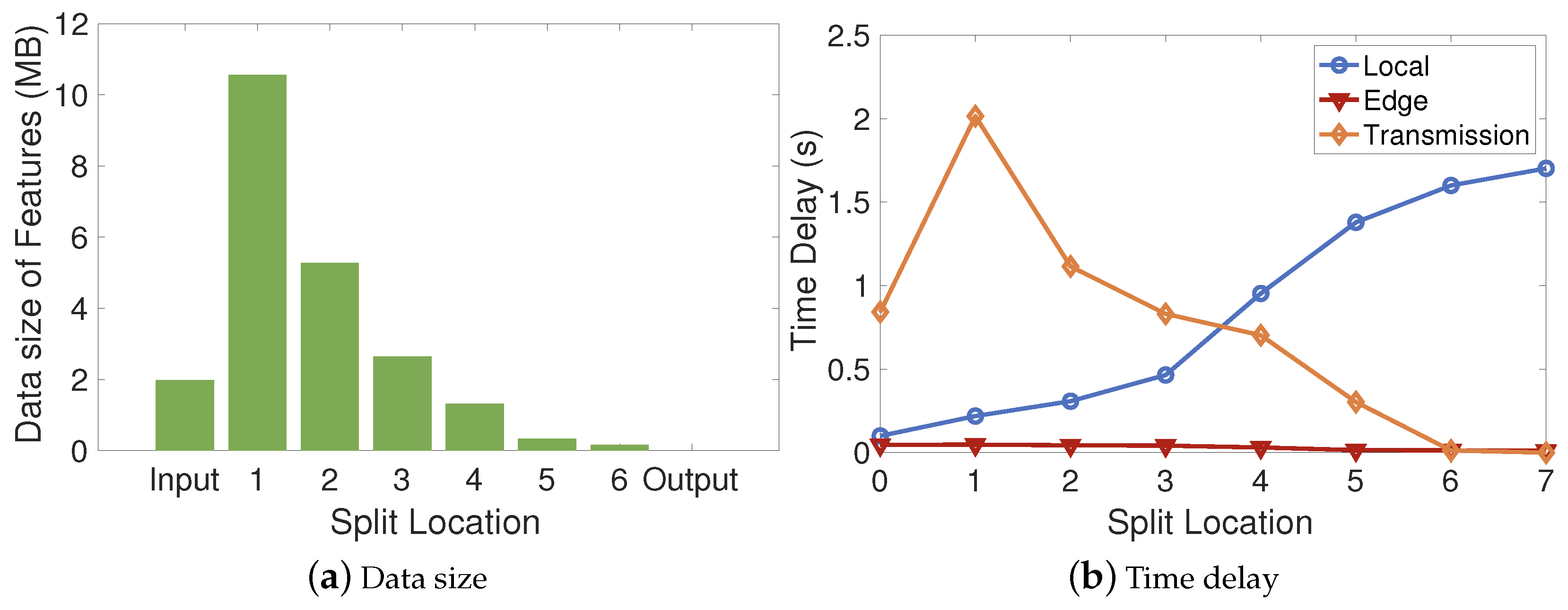
Figure 1. The output data size and inference delays at different split locations.
Make 07 00117 g001
Figure 2. System architecture of DNN-Scissor. The local device reads a video frame from the camera. DNN-Scissor determines where to split the DNN model to distribute the feed-forward calculations to the local device and edge. The local device feed-forwards from the first layer and stops at the split location and then transmits the intermediate features to the edge through a network, and the edge continues the feed-forward calculations for the rest of the DNN layers.
Make 07 00117 g002
Figure 3. Candidate splitting locations on YOLOv3. The circled numbers indicate a total of 8 candidate locations to split YOLOv3. Each of the locations, 1 to 4, can split the network layers into two blocks with one intermediate 3D feature map. Each of the locations, 5 to 6, splits the three branches in parallel, resulting in three intermediate 3D feature maps.
Make 07 00117 g003
Figure 4. Deep reinforcement learning framework to learn DNN splitting policy.
Make 07 00117 g004
Figure 5. A2C framework to learn the policy of splitting DNNs.
Make 07 00117 g005
Figure 6. System testbed for experiments.
Make 07 00117 g006
Figure 7. Candidate splitting locations (with circled numbers) on ResNet18 and AlexNet. (a) The candidate split locations of ResNet18 are between every residual block, so each location can break the network into two parts and result in one block of intermediate feature matrices. (b) The candidate split locations of AlexNet are between every convolution block and every fully connected (FC) layer.
Make 07 00117 g007
Figure 8. Traffic videos for testing.
Make 07 00117 g008
Figure 9. Performance comparison of all the methods. DNN-Scissor achieves the shortest total delay and the minimum system cost among all the methods.
Make 07 00117 g009
Figure 10. Performance comparison of all the methods with varying network bandwidths for segmenting YOLOv3. With the increase in bandwidth, total delay, drop rate, and system costs slightly decrease in all the methods.
Make 07 00117 g010
Figure 11. Effects of trade-off weight w. With the increase in data weight, the average data amount to be transmitted deceases, but the total delay increases for each DNN segmentation.
Make 07 00117 g011
Figure 12. Effects of video frame reading rate. With the increasing reading rate, the total delay and drop rate decreases, but the amount of transmitted data slightly increases.
Make 07 00117 g012
Figure 13. Reward convergence when segmenting different DNNs.
Make 07 00117 g013
Table 1. Details of DNNs to be segmented.
DNNSize# ParametersLocal Inference TimeEdge Inference Time
YOLOv3236 MB61.53 M4.347 s0.759 s
ResNet1844.6 MB11.7 M0.187 s0.5 s
AlexNet233 MB62.37 M0.136 s0.616 s
Table 2. Percentage improvement of DNN-Scissor over baseline methods for YOLOv3.
Metricvs. LocalOnlyvs. EdgeOnlyvs. SemiFixedvs. Greedy
Transmitted Data Amount NA49%−66%26%
Total Delay Reduction86%25%77%83%
Drop Rate Reduction56%−68%6%30%
System Cost Reduction63%42%50%67%
Table 3. Inference output of AlexNet on a sample image across different partitioning configurations.
Partitioning StrategyTop 1 Predicted ClassTop 1 Logit Value
No Partition (Executed Locally)‘golden retriever’9.3985
Split at Layer 2‘golden retriever’9.3985
Split at Layer 5‘golden retriever’9.3985
Split at Layer 8‘golden retriever’9.3985
No Partition (Executed on Edge)‘golden retriever’9.3985
Table 4. Empirical latency breakdown (in ms) for YOLOv3 under different learned policies, reflecting adaptation to network conditions.
Learned Policy:Split PointLocal Comp.Trans.Edge Comp.Total Delay
High BandwidthShallow (e.g., 2)260145390795
(Low w policy) (33%)(18%)(49%)
Low BandwidthDeep (e.g., 4)1150481651363
(High w policy) (84%)(4%)(12%)
Table 5. Video frame reading rates for the three DNNs.
DNNIIIIII
YOLOv3800 ms1000 ms1200 ms
ResNet18100 ms150 ms200 ms
AlexNet100 ms150 ms200 ms
Disclaimer/Publisher’s Note: The statements, opinions and data contained in all publications are solely those of the individual author(s) and contributor(s) and not of MDPI and/or the editor(s). MDPI and/or the editor(s) disclaim responsibility for any injury to people or property resulting from any ideas, methods, instructions or products referred to in the content.