Article

Leveraging DNA-Based Computing to Improve the Performance of Artificial Neural Networks in Smart Manufacturing

Division of Mechanical and Electrical Engineering, Kitami Institute of Technology, 165 Koen-cho, Kitami 090-8507, Japan
*
Authors to whom correspondence should be addressed.
Mach. Learn. Knowl. Extr. 2025, 7(3), 96; https://doi.org/10.3390/make7030096
Submission received: 7 July 2025 / Revised: 24 August 2025 / Accepted: 4 September 2025 / Published: 9 September 2025

Abstract

Bioinspired computing methods, such as Artificial Neural Networks (ANNs), play a significant role in machine learning. This is particularly evident in smart manufacturing, where ANNs and their derivatives, like deep learning, are widely used for pattern recognition and adaptive control. However, ANNs sometimes fail to achieve the desired results, especially when working with small datasets. To address this limitation, this article presents the effectiveness of DNA-Based Computing (DBC) as a complementary approach. DBC is an innovative machine learning method rooted in the central dogma of molecular biology that deals with the genetic information of DNA/RNA to protein. In this article, two machine learning approaches are considered. In the first approach, an ANN was trained and tested using time series datasets driven by long and short windows, with features extracted from the time domain. Each long-window-driven dataset contained approximately 150 data points, while each short-window-driven dataset had approximately 10 data points. The results showed that the ANN performed well for long-window-driven datasets. However, its performance declined significantly in the case of short-window-driven datasets. In the last approach, a hybrid model was developed by integrating DBC with the ANN. In this case, the features were first extracted using DBC. The extracted features were used to train and test the ANN. This hybrid approach demonstrated robust performance for both long- and short-window-driven datasets. The ability of DBC to overcome the ANN’s limitations with short-window-driven datasets underscores its potential as a pragmatic machine learning solution for developing more effective smart manufacturing systems, such as digital twins.

1. Introduction

Smart manufacturing, also known as Industry 4.0/5.0, represents a transformative leap in the evolution of manufacturing within the scope of the fourth/fifth industrial revolution [1,2]. It harnesses the power of information and communication technologies (ICT) to tackle manufacturing problems. Among others, its main constituents are Human–Cyber–Physical Systems (HCPS) [3,4], Industrial Internet of Things (IIOT) [5], Big Data (BD) [6,7,8], Open Data [9], Data Analytics [6,7], Machine Learning (ML) [10], Digital Twins (DTs) [11,12], Network Control Systems (NCS) [13], Sensor Signals and Signal Processing Techniques [14], and Digital Manufacturing Commons (DMC) [7,8,9,15]. These constituents are embedded into manufacturing enablers such as machine tools, human resources, peripherical equipment, enterprise resources planning systems, computer-aided design/manufacturing/process planning systems, and supply chain systems to drive automation and autonomy. Consequently, these enablers must support cognitive tasks like monitoring (what is happening), understanding (why it is happening), predicting (what may happen), deciding (choosing an appropriate action), and adapting (implementing the decision) in real time. All these constituents and enablers interact within a data-driven workflow to achieve the abovementioned tasks, as shown in Figure 1.
As seen in Figure 1, manufacturing activities generate diverse data streams, such as sensor signals. These raw data are subsequently wrangled—often with semantic annotation—so they are structured, human- and machine-readable, and stored in local or cloud databases for stakeholder access [7,8,9]. For instance, as seen in Figure 1, to perform cognitive tasks like monitoring and prediction, features (typically derived from time, frequency, time–frequency, or delay domains [14,16,17,18,19]) are extracted from the stored datasets and then utilized for machine learning. The resulting machine-learned models are then adapted by the enablers [10,12,20,21], and feedback from operations can be used to update or retrain or the models as conditions evolve.
Within the abovementioned workflow, bioinspired computing methods—a facet of biologicalization in manufacturing [22,23,24]—are increasingly used to improve adaptability and learning. These methods such as Artificial Neural Networks (ANN), Evolutionary Algorithms, and Swarm Intelligence mimic biological systems to solve problems. For instance, an ANN, inspired by the human brain’s operation, can analyze sensor data, detect underlying patterns, and predict equipment failures and/or process anomalies. Evolutionary Algorithms (e.g., Genetic Algorithms (GAs), Genetic Programming (GP), and Differential Evolution (DE)), inspired by biological evolution processes (reproduction, mutation, recombination, and selection), can optimize processes like scheduling or resource allocation. Swarm Intelligence algorithms (e.g., Particle Swarm Optimization (PSO), Ant Colony Optimization (ACO), and Bat Algorithm (BA)), inspired by the collective behavior of birds, animals, and insects, can functionalize decentralized decision-making and improve coordination among autonomous systems. Among these, the ANN and its derivatives are widely used in manufacturing, particularly for tasks such as pattern recognition in sensor data, and thus enabling real-time anomaly detection and deciding corrective measures on time [10,12,18,19]. However, this is challenging to materialize in extreme conditions, such as when few data are available due to a short window [25].
The signal window size is a crucial factor in analytics, influencing both granularity and responsiveness. A short window, for instance, enables faster detection of anomalies, which is crucial in environments where machinery faults can lead to immediate production disruptions. However, it often results in poorer feature resolution, which can hinder the ability to detect and analyze characteristic components of the signal [25]. On the other hand, a long window enhances the feature resolution and stability of the analysis [26]. However, it may delay detecting changes and anomalies, leading to slower responses to critical events. Researchers continue to investigate these trade-offs, exploring adaptive methods and optimal window sizes across domains. Section 2 reviews related work, including studies that rely on long windows without explicitly analyzing the effect of window size.
In essence, across different domains such as healthcare, manufacturing, energy consumption, and others, statistical ML methods (e.g., Support Vector Machine (SVM), k-Nearest Neighbors (K-NN), and Random Forest (RF)) and bioinspired methods (e.g., ANN, Long Short-Term Memory (LSTM), Gated Recurrent Unit (GRU), and Convolutional Neural Network (CNN)) are widely used for pattern recognition and prediction. Studies [10,18,23,26,27,28,29,30,31] consistently demonstrate that these methods perform better with longer windows, enhancing feature resolution and classification accuracy. Yet, there remains a need for methods that can handle smaller datasets or shorter windows, especially for rapid detection in manufacturing fault diagnosis. Current research explores ensemble techniques and optimized window sizes to address these challenges.
Building on the ongoing exploration, this study seeks to extend the current understanding by focusing on the performance of ANNs under short data windows (approximately 10 data points). Since ANNs struggle to maintain accuracy in this context, this study introduces another bioinspired method called DNA-Based Computing (DBC) [23,30,32], in combination with the ANN, and assesses their efficacy. By exploring these configurations, the study sheds some light on alternative strategies for pattern recognition and prediction capabilities when data are scarce. The study therefore contributes to adapting cognitive processing methods for data-constrained environments, supporting rapid recognition and corrective action.
Figure 2 schematically illustrates this study’s context. As seen in Figure 2, this study considers time series datasets subjected to “Normal” and “Abnormal” patterns. The datasets are further segmented into long- and short-window sets. Two approaches are then applied on the datasets: a traditional approach using time-domain feature engineering with the ANN and a non-traditional approach using DBC with the ANN. The objective is to compare their performance in recognizing the pattern-types (Normal/Abnormal).
For a better understanding, the remainder of this article is structured as follows. Section 2 provides a succinct review of the relevant studies. Section 3 describes data preparation. Section 4 describes the traditional and non-traditional approaches. Section 5 presents and discusses the results. Section 6 provides the concluding remarks of this study. For clarity, Appendix A provides a glossary of symbols related to Section 3 and Section 4. Appendix B presents the pseudocode for the feature extraction process, while Appendix C includes the pseudocode for the feature selection process. Appendix D describes the pseudocode for machine learning, and Appendix E outlines the central dogma of molecular biology. Finally, Appendix F presents the Type-2 DNA-based computing (DBC).

2. Literature Review

As outlined in Section 1, signal window size is a key factor influencing the granularity and responsiveness of deployed analytics, including signal processing, bioinspired computing, and statistical ML methods. To provide a comprehensive overview of the current research trends and highlight gaps, this section is divided into two parts. Section 2.1 reviews studies that analyze trade-offs between window size and adaptive methods. Section 2.2 reviews studies that use long window data without critically addressing window size.

2.1. Studies Related to Analyzing the Role of Window Size

Many studies have examined how window size affects recognition accuracy, responsiveness, and resource efficiency. These works span domains such as healthcare, manufacturing, and smart sensing, often comparing multiple ML or bioinspired algorithms. A common theme is balancing short windows, which enable timely detection, with long windows, which improve feature extraction. Some researchers also propose adaptive strategies that dynamically adjust window size to signal behavior. Some of these works are briefly described below.
Wahid et al. [26] explored how increasing window size improves gesture recognition using electromyography (EMG) signal datasets. The authors demonstrated a direct link between long windows and improved classification accuracy of different ML algorithms such as K-NN, Linear Discriminant Analysis, Logistic Regression, Naïve Bayes, SVM, and RF.
Alyammahi and Liatsis [33] explored nonintrusive load monitoring (NILM) by proposing a method that uses time-domain features across various window sizes to identify active electrical appliances from aggregated power signals. The authors highlighted the critical role of determining the optimal window size and adapting ML algorithms like K-NN, Bagged Trees, and Boosted Trees for adequate power consumption disaggregation. They underscored the necessity of refining window size and classifier settings to enhance performance in NILM tasks.
Kausar et al. [27] addressed the challenge of differentiating falls from regular activities in older adults by developing a wearable device that utilizes feature extraction methods on accelerometry data. The authors emphasized the significance of selecting an optimal window size for processing time and detection efficacy, exploring the performance of ML and bioinspired algorithms such as SVM, K-NN, RF, and ANN in classifying these movements. They demonstrated that a window size of three (3) seconds offers a balanced approach, and the combination of SVM and RF algorithms shows high accuracy and robustness in fall detection.
Feiner et al. [34] presented a framework for real-time detection of the operating states of a forklift. The framework classifies acceleration data through a windowing approach, deploying various ML algorithms. The authors articulated that selecting an appropriate window size is essential to enhance the detection system’s accuracy.
Clerckx et al. [35] discussed the impact of window size on signal processing efficiency from the viewpoint of wireless sensor networks used in industrial settings. The authors underscored that the right window size is vital for optimizing data transmission and minimizing interference, resulting in reliable and efficient communication within these networks. They also articulated that adaptive strategies for window sizing can significantly enhance the performance and stability of industrial wireless sensor systems.
Batool et al. [31] investigated the performance of ensembled bioinspired methods to analyze temporal data from wearable sensors, focusing on applications in healthcare, sports, and surveillance. They also presented a hybrid LSTM- GRU model, derivatives of ANN, to enhance human activity recognition. This model employs a strategic data windowing technique, segmenting sensor data into frames of 128 timestamps with 50% overlap.
Cuentas et al. [36] articulated that window size significantly influences the pattern recognition performance of statistical ML and bioinspired algorithms in the control chart pattern recognition (CCPR) paradigm in manufacturing. The authors described that a short window results in higher false recognition rates. On the other hand, a long window helps decrease the false recognition rates, increasing the detection time. The authors also presented an SVM-GA model for optimizing the pattern recognition tasks, where a window size of 25 is the optimal choice.
Maged and Xie [28] explored the efficacy of a CNN combined with adaptive boosting capability for recognizing abnormal patterns in manufacturing settings. The authors tested its (CNN with adaptive boosting) correct recognition rate (CRR) for different window sizes (25, 30, 35, 40, and 45). The model achieves higher CRR with increasing window sizes and even achieves a perfect CRR with a window size of 40.
Derakhshi and Razzaghi [37] introduced a Bi-directional LSTM model, a derivative of ANN, for CCPR in manufacturing settings. The model handles the inherent class imbalance by implementing an adaptive weighting strategy and a bi-objective early stopping technique. It also employs a rolling window-based metric to assess the stability of CCPR classifiers and select an optimal window size.
Ullah [30] argued that most CCPR-centric works consider long window sizes. The author underscored the importance of developing methods to handle data subjected to relatively shorter window sizes (more or less 15 data points), enabling corrective measures on time in a manufacturing environment. The author also introduced a bioinspired computing method based on the central dogma of molecular biology and demonstrated its efficacy in CCPR when the window is relatively short [23,30], image processing [23,32] and tool wear prediction and pattern recognition [38,39].

2.2. Studies Related to Using Long Window Data

In contrast, a separate body of work applies signal analytics assuming large data volumes, often using fixed long windows without critically examining their effects. These studies highlight the strength of multi-sensor fusion, deep learning, and statistical feature extraction but generally overlook adaptability under data scarcity. Some of these works are briefly described below.
Caggiano and Nele [40] described a multi-sensor-based system utilizing ANN to predict tool wear while drilling carbon fiber-reinforced plastic (CFRP) stacks, commonly used in aerospace fuselage panels. The system integrates multiple sensor inputs like thrust force, torque, and acoustic emissions, processes them, and fuses them to predict tool conditions.
Haoua et al. [29] introduced a system for material detection in electric automated drilling units (eADU) used for aerospace component assembly, where multi-material stacks like CFRP, titanium, and aluminum alloys pose distinct machining challenges such as delamination and roughness. The system utilizes an RF-based ML model combined with multi-sensor data fusion and frequency domain-based data processing techniques.
Segreto and Teti [10] developed an ANN-based approach to automate the decision-making process for stopping robot-assisted polishing operations. This approach incorporates statistical feature extraction and principal component analysis (PCA) to analyze sensor signals and classify polishing process states.
Guo et al. [41] introduced an LSTM-based prediction system for estimating surface roughness in the grinding process. The system processes grinding force, vibration, and acoustic emission signals, extracting numerous features in both time and frequency domains.
Lee et al. [42] introduced a Kernel PCA-driven method for tool condition monitoring (TCM) in milling. The method uses Kernel Density Estimation (KDE)-based T2-statistic and Q-statistic control charts and multi-sensor signals (current, acoustic emission, and vibration acceleration signals) at a minimum sampling frequency of 100 kHz.
Jáuregui et al. [17] presented a method for TCM in high-speed micro-milling, incorporating multi-sensor-signals (cutting force and vibration signals). The method performs frequency and time-frequency analysis of signals, acquired at a sampling frequency of 38,200 Hz and 89,100 Hz, respectively.
Zhou and Xue [43] introduced a multi-sensor feature extraction method for TCM in milling. The method integrates time, frequency, and time-frequency domain analyses for feature extraction and employs a Kernel-based Extreme Learning Machine (KELM) and a modified GA for prediction purposes.
Hameed et al. [20] introduced a multi-sensor approach for predicting the tools’ remaining useful life (RUL) in gear hobbing. This approach uses multi-sensor signal datasets (temperature, current, and vibration signals) and a multi-layer ANN for prediction purposes.
Bagga et al. [44] presented an ANN-based tool wear prediction system. The system analyzes images captured from worn tools during machining processes (carbide inserts cutting AISI 4140 steel under dry conditions) along with parameters like cutting speed, feed, and depth of cut to predict flank wear and RUL.
Teti et al. [18] introduced a multi-sensor process monitoring system to make informed decisions regarding the timing of tool changes while drilling CFRP laminate stacks. The system acquires thrust force and torque signals while drilling, extracts various features (time domain, frequency domain, and fractal domain features) from the acquired signals, and feeds the features to an ANN to make informed decisions.
Segreto et al. [19] developed an ANN-based system to predict surface roughness while polishing steel bars. The system acquires acoustic emission, strain, and current measurement signals, extracts time and frequency domain features, and feeds the extracted features to an ANN for prediction.
In summary, across domains, statistical ML and bioinspired methods are widely applied for pattern recognition and prediction. These methods perform better with longer windows. However, there is a critical need for techniques that remain effective with small datasets or short windows, where rapid detection and corrective action are vital. Current research actively explores strategies such as ensemble multiple methods and optimizing window sizes to address these challenges. This study builds on these efforts by examining ANN performance under very short windows (as few as 10 data points). Recognizing ANN’s limitations, this study further integrates another bioinspired method, DNA-Based Computing (DBC), in conjunction with the ANN to improve recognition, as outlined in Section 1. As such, the following section describes the relevant data preparation method.

3. Data Preparation

As outlined in Section 1, this study considers time series datasets subjected to “Normal” and “Abnormal” patterns. As such, this section describes the datasets and their preparation.
The Normal and Abnormal patterns in this study follow the framework of CCPR, a standard approach in manufacturing quality control [30,36,37]. Normal patterns represent in-control behavior, where process variability remains within expected limits and operations are stable. Abnormal patterns—such as shifts, trends, cycles, mixtures, and sudden spikes—represent signal deviations from stability and often correspond to tool wear, misalignment, fluctuating feed rates, or other disturbances in production. Recognizing these patterns quickly is critical for preventing quality loss and unplanned downtime, as they provide early warnings of underlying faults. The datasets used here are therefore directly relevant to manufacturing practice, capturing both stable process dynamics and fault-indicating behaviors that demand corrective action. In this way, they provide a meaningful basis for evaluating how different machine learning approaches, such as ANN and DBC, perform under both normal and fault conditions.
As outlined in Table 1, 100 (one hundred) time series datasets are generated—50 Normal and 50 Abnormal—following the definitions in [30]. Let the set of these datasets be denoted as Z = {Zk | k = 1, …, 100}. Each Zk in Z is a series of points such as Zk = {Zk(i) | i = 0, …, N}, where N is the window size. The specific definitions and mathematical formulations of Normal/Abnormal patterns are beyond the scope of this study and can be found in [30].
The generated datasets (Z) are made publicly available in text format (*.txt) via a GitHub repository. One may access them using the URL: https://github.com/commons-repo/001-research-data.git (accessed on 20 August 2025). One may also access them via the GitHub CLI (command line interface) using the command: gh repo clone commons-repo/001-research-data.
As outlined in Table 1, equal and mutually exclusive sets of training and test datasets are then created from the Z. Here, training datasets refer to the datasets to be used in the subsequent phases of this study for machine learning. On the other hand, test datasets refer to the datasets to be used in the subsequent phases of this study for evaluating the performance of the machine-learned models. Let the sets of training and test datasets be denoted as X and Y, respectively. As such, {X, Y} ⊂ Z, where |X| = |Y| = 50 and XY = ∅. The pattern ratio in X and Y is preserved as in Z.
As outlined in Table 1, X and Y then undergo long- and short- windowing. Here, long-windowing means changing the window size N to Nl(=150) for each dataset in X and Y. Short-windowing means changing the window size N to Ns(=10) for each dataset in X and Y. This results in long window training datasets, short window training datasets, long window test datasets, and short window test datasets. Let the sets of these datasets be denoted as Xl, Xs, Yl, and Ys, respectively.
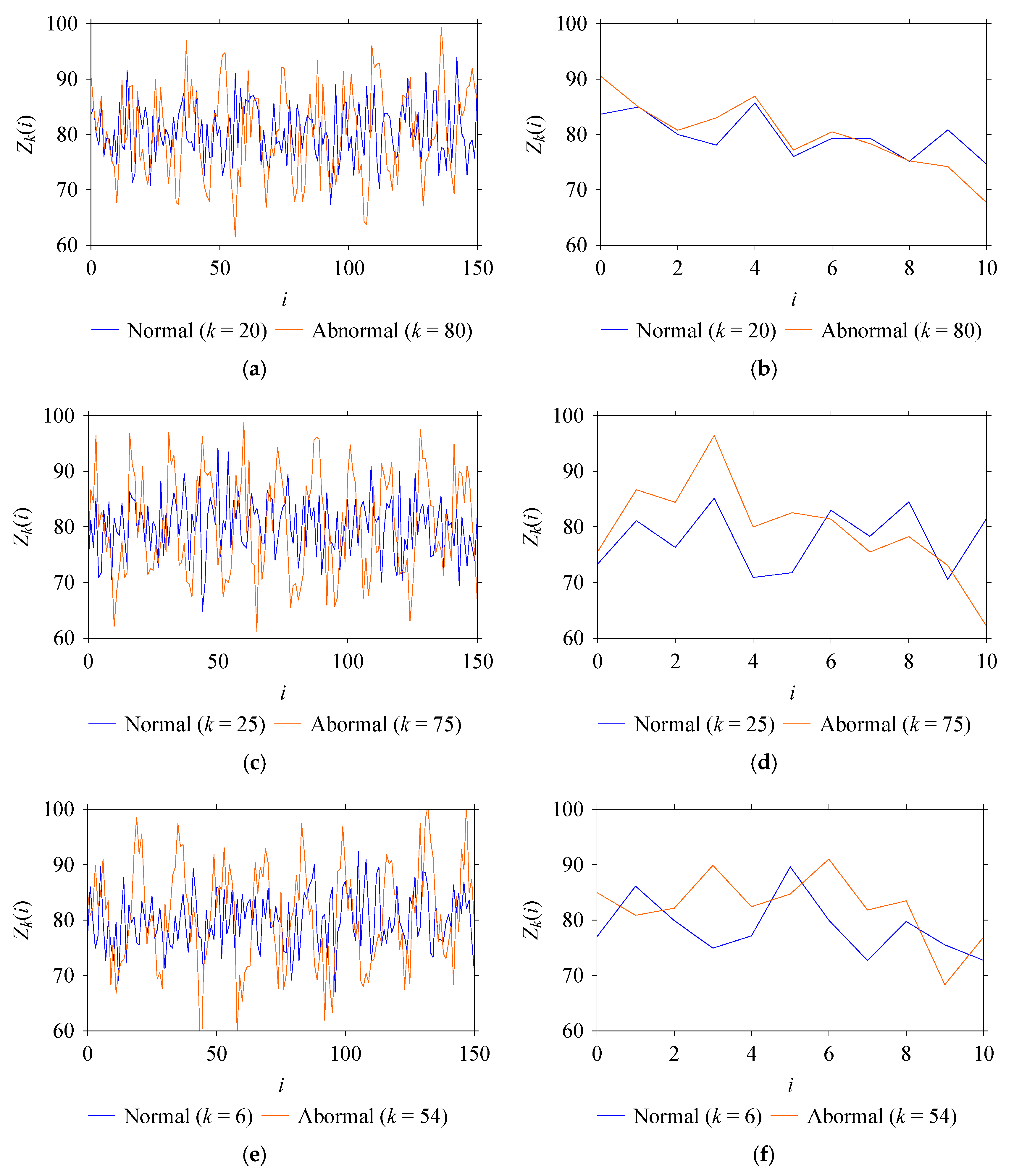
Figure 3 shows some instances of the prepared long and short window datasets. As seen in Figure 3, when a long window time series (see Figure 3a,c,e) is considered, the normal and abnormal patterns can be distinguished easily. However, this is not the case when the window is kept short for the same time series datasets (see Figure 3b,d,f). As seen in Figure 3b,f, a normal pattern might appear to behave like an abnormal pattern, showing similar dynamics. This means that a short-windowed signal might be difficult to handle compared to that of a long window for the sake of recognizing underlying patterns.
Nevertheless, as mentioned in Section 1, the prepared datasets (Xl, Xs, Yl, and Ys) undergo two distinct approaches for the sake of evaluating pattern recognition performance of a ANN. The following section describes these approaches.

4. Methodology

This study investigates the performance of an ANN in pattern recognition under the constraints of shorter data windows. Two approaches are considered: a traditional approach using time-domain feature engineering, and a non-traditional approach using DNA-Based Computing (DBC). Both are applied to the datasets described in Section 3. The relevant methodologies underlying the approaches are described in the following subsections, Section 4.1 and Section 4.2, respectively.

4.1. Traditional Approach

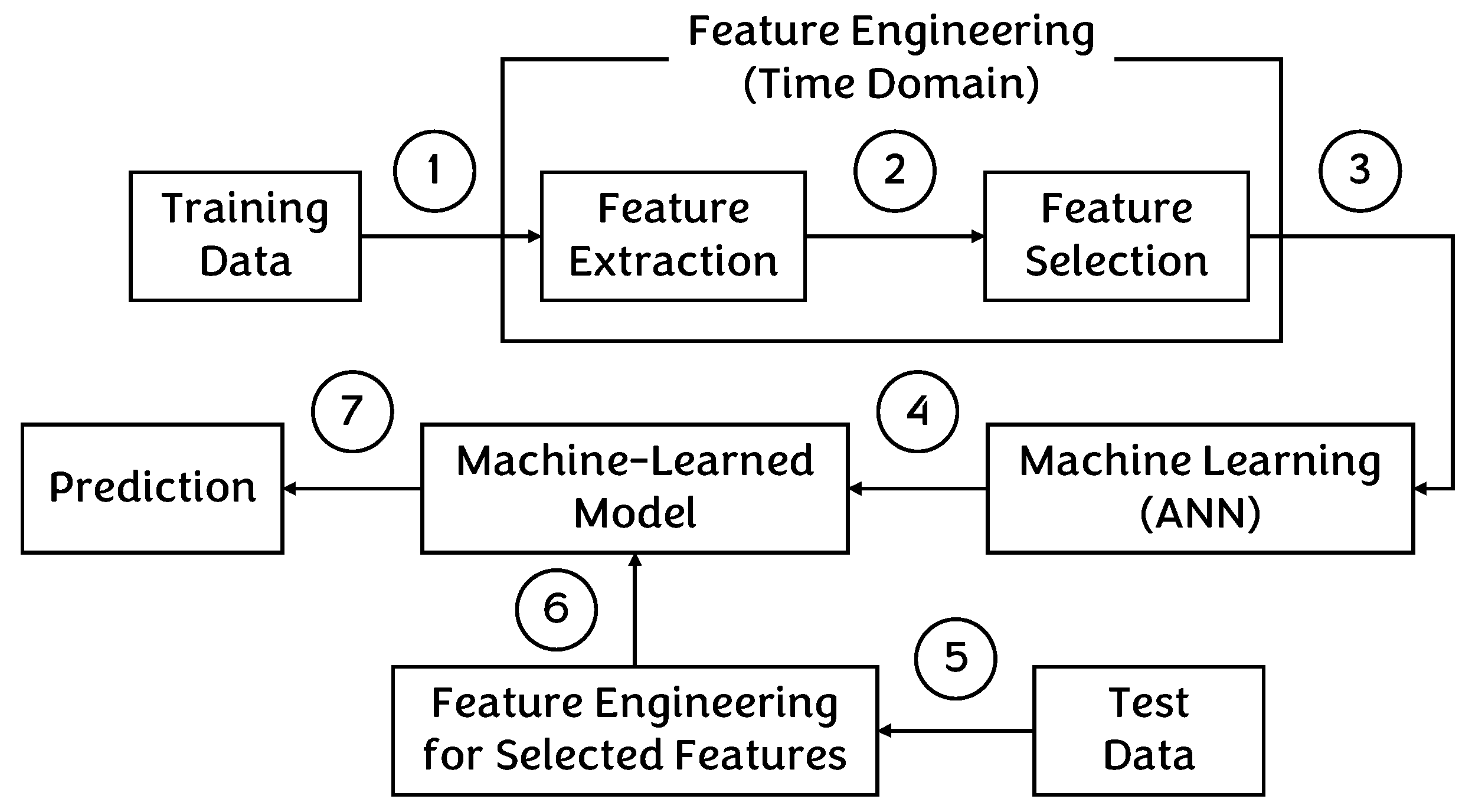
Figure 4 schematically illustrates the traditional approach, integrating time domain featuring engineering and ANN, for the sake of pattern recognition.
As seen in Figure 4, first, statistical time domain features are extracted from both the long/short window training datasets (Xl and Xs, respectively). Let the extracted features sets relevant to Xl and Xs be denoted as Fl and Fs, respectively. This can be expressed as follows. Fl: Xl → Feature Space, Fs: Xs → Feature Space, Fl = {Flj|j = 1, …, 7}, and Fs = {Fsj|j = 1, …, 7}. Here, Fl1 = Fs1 = Average, Fl2 = Fs2 = Standard Deviation, Fl3 = Fs3 = Minimum Value, Fl4 = Fs4 = Maximum Value, Fl5 = Fs5 = Range, Fl6 = Fs6 = Skewness, and Fl7 = Fs7 = Kurtosis. Note that Appendix B provides supporting materials: Table A2 presents pseudocode outlining this feature extraction process, and Table A3 provides a minimal MATLAB® (version R2024b) code skeleton illustrating the same implementation.
Subsequently, as seen in Figure 4, prominent features in Fl and Fs are selected. This step is particularly significant for reducing the number of features and enhancing the predictive performance by focusing on the most informative ones. For this, a well-known feature selection technique called Random Forest (RF) [26,27,29], is employed. In particular, RF is implemented using MATLAB®’s TreeBagger function in classification mode, with 30 trees (a commonly used choice for small- to medium-sized datasets) and all other parameters kept at their default settings. Feature importance is evaluated using the out-of-bag (OOB) permutation method: prediction error is first measured on the OOB samples, then each feature is randomly shuffled to break its relationship with the target. The increase in error caused by this shuffling indicates how strongly the model depends on that feature. A larger increase means the feature is more important, while a smaller increase suggests it contributes less to classification performance. This provides a straightforward way to rank features according to their contribution to classification. Note that Appendix C provides supporting materials: Table A4 presents pseudocode outlining this feature selection process, and Table A5 provides a minimal MATLAB® (version R2024b) code skeleton illustrating the same implementation, along with the official documentation URL for the TreeBagger function. The outcome of this selection process is two new sets of selected features from Fl and Fs. Let these sets be denoted as Fltrain and Fstrain, respectively, where FltrainFl and FstrainFs.
As seen in Figure 4, the selected features, Fltrain and Fstrain, are then used for machine learning, particularly to train an ANN. For this, Fltrain is fed into a two (2)-layer feed-forward ANN, a commonly used pattern recognition ANN available in the MATLAB® Neural Net Pattern Recognition App. The first layer (hidden layer) of the ANN utilizes sigmoid neurons, which are adept at handling even non-linear data transformations. The second layer (output layer) of the ANN utilizes softmax neurons to classify the inputs into probabilistic outputs corresponding to each pattern. The number of neurons in the hidden layer is set to three (3). Note that Appendix D provides supporting materials: Table A6 presents pseudocode outlining this training process, and Table A7 provides a minimal MATLAB® (version R2024b) code skeleton illustrating the same implementation, along with the official documentation URL for the pattern recognition ANN. As such, this ANN machine-learns from the Fltrain and generates a trained ANN model. Let the model be denoted as ANN1, a machine-learned model for long window datasets. Similarly, Fstrain is also fed into the same configuration ANN, resulting in another trained model. Let this model be denoted as ANN2, a machine-learned model for short window datasets.
As seen in Figure 4, the trained models, ANN1 and ANN2, undergo performance tests for pattern recognition. For this, as seen in Figure 4, features are extracted from long and short window test datasets (Yl and Ys). Let these feature sets be denoted as Fltest and Fstest, respectively. Fltest and Fstest are identical to the Fltrain and Fstrain, respectively. This can be expressed as follows. f (Fltest(j)) = Fltrain(j) and Fltest(j)Fltrain(j). f (Fstest(j)) = Fstrain(j) and Fstest(j)Fstrain(j). Fltest and Fstest are then fed into the corresponding ANN models, ANN1 and ANN2, evaluating the models’ performance in predicting the patterns (normal and abnormal) underlying Yl and Ys, respectively. Note that the feature extraction step for the test datasets follows the same pseudocode and code skeleton provided in Appendix B. Furthermore, for the testing phase, Appendix D provides the supporting materials like the training phase.

4.2. Non-Traditional Approach

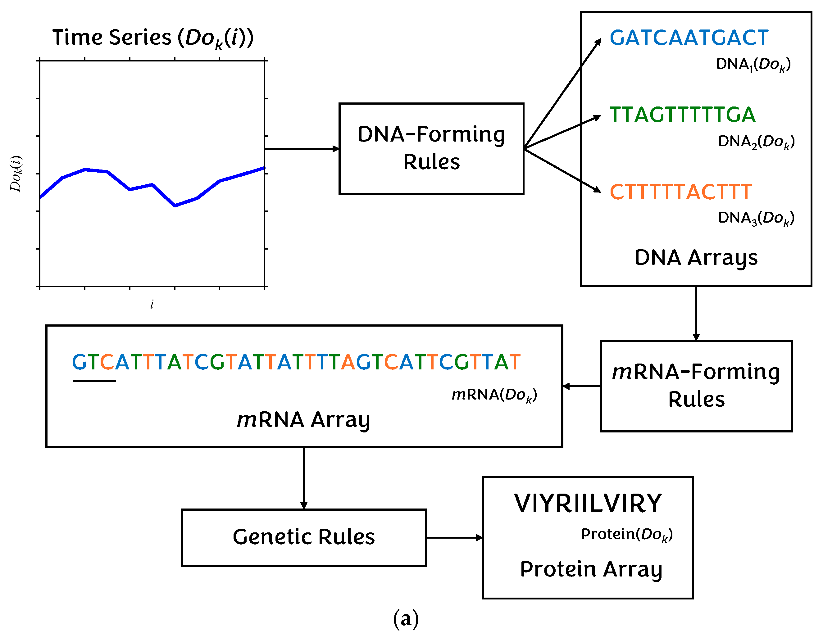
Figure 5 schematically illustrates the non-traditional approach, integrating DNA-Based Computing (DBC) and ANN, for the sake of pattern recognition.
DBC is inspired by the “central dogma of molecular biology,” a principle that biological organisms follow. As described in Appendix E, according to this principle, information flows from DNA or RNA to protein, not from protein to DNA or RNA [23,32,45]. Since DNA/RNA are 4-element pieces of information and proteins are 20-element pieces of information, the central dogma of molecular biology eventually refers to creating many-element pieces of information (protein-type) from few-element pieces of information (DNA- and RNA-type). This metaphor forms the conceptual foundation of the DNA-Based Computing (DBC) framework. The DBC can take different forms depending on the problem to be solved. Nevertheless, the DBC form suitable for signal-based ML is type-2 DBC [23]. This study also adapts this form.
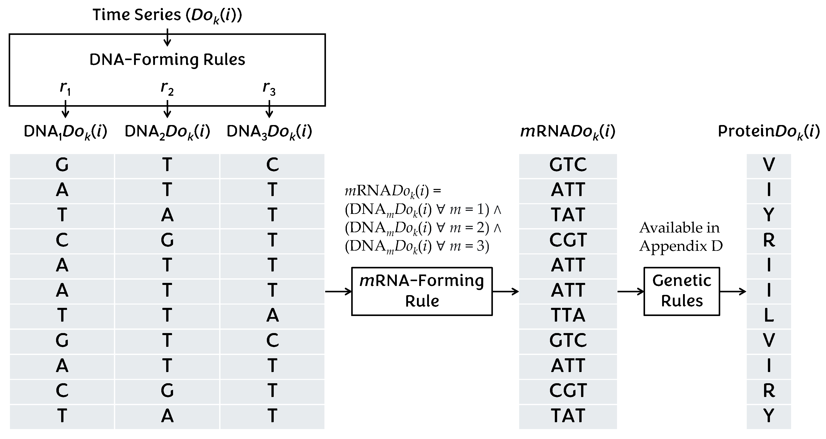
As seen in Figure 5a, the type-2 DBC first receives a time series dataset, denoted as Dok(i), where D ∈ {X,Y}, o ∈ {l,s}, k = {1, …, 100}, i = {0, …, No}. The dataset is then converted into three (3) DNA arrays, using three different DNA-forming rules, say r1, r2, and r3, as described in [30]. As such, DNA arrays obtained for a dataset can be expressed as: DNAm(Dok) = {DNAm(Dok(i))}, where DNAm(Dok(i)) = rm=1,2,3(Dok(i)). Consequently, the DNA arrays collectively generate a mRNA array, following a mRNA-forming rule. This can be expressed as: mRNADok(i) = (DNAmDok(i) ∀ m = 1) ∧ (DNAmDok(i) ∀ m = 2) ∧ (DNAmDok(i) ∀ m = 3). Hence, mRNADok(i) is basically 3-letter symbol codons, generated from the corresponding DNA array elements. As seen in Figure 5a, these codons are then translated to a 1-letter symbol of an amino-acid (or protein), using the genetic rules denoted as g, as described in [22]. This can be expressed as: ProteinDok(i) = g(mRNADok(i)). This eventually results in protein arrays, which can be expressed as: ProteinDok = {ProteinDok(i)}. Note that the definition of the abovementioned rules (r1, r2, r3, and g) and related mathematical formulations are beyond the scope of this study. One may refer to the work described in [30] for details. Additionally, the abovementioned type-2 DBC for generating protein arrays from time series datasets are also thoroughly described in [23,30]. One may refer to these works for details.
Figure 5b shows how the abovementioned DBC is integrated with the ANN for the sake of pattern recognition. As seen in Figure 5b, DBC is introduced instead of traditional time domain feature engineering, compared to the traditional approach (described in Section 4.1, can also be seen in Figure 4).
As seen in Figure 5b, both the long/short window training datasets (Xl and Xs, respectively) first undergo the abovementioned DBC, resulting in protein arrays. The generated protein arrays are then quantified, calculating the relative frequencies of amino-acids available in an array. Let “P” be the set of all possible amino-acids encoded in a protein array (ProteinDok), “p” be an amino-acid which is part of the “P”, “Cp” be the number of times “p” appears in “P”, and “C” be the total number of proteins in “P”. As such, the calculated relative frequencies for a protein array can be expressed as: RF(p) = Cp/C, pP. This results in a set of relative frequencies for a dataset (recall each dataset in Xl and Xs), which can be expressed as: RFDok = {RF(p), pP}. This further results in aggregated sets of relative frequencies, which can be expressed as: RFDo = {RFDok}. Hence, sets denoted as RFXl and RFXs are generated for Xl and Xs, respectively. These sets become DBC-driven features for the subsequent analyses.
As seen in Figure 5b, these features (RFXl and RFXs), are then used for training the pattern recognition ANN. The method and ANN configurations are the same as those of the traditional, as described in Section 4.1. As such, the ANN machine-learns from the RFXl and generates a trained ANN model. Let the model be denoted as ANN3, a DBC-based machine-learned model for long window dataset. Similarly, the ANN machine-learns from RFXs, resulting in another trained model. Let this model be denoted as ANN4, a DBC-based machine-learned model for short window datasets.
As seen in Figure 5b, DBC-driven features from both the long/short window test datasets (Yl and Ys, respectively) are calculated similarly as before. Let these sets be denoted as RFYl and RFYs, respectively. These are then fed into the corresponding ANN models (ANN3 and ANN4), evaluating the models’ performance in predicting the patterns underlying Yl and Ys, respectively.
For clarity, Appendix F provides a worked example of type-2 DBC applied to an actual time series dataset. This example illustrates each stage in detail, complementing the schematic explanation in Figure 5 and above description. Furthermore, the source code for type-2 DBC has been made available through a GitHub repository. Appendix F provides access details as well.
The following section presents and discusses the results obtained from the abovementioned approaches.

5. Results

The results are presented and discussed in two parts. In particular, Section 5.1 and Section 5.2 present and discuss the results for traditional approach (described in Section 4.1) and non-traditional approach (described in Section 4.2), respectively.

5.1. Results for Traditional Approach

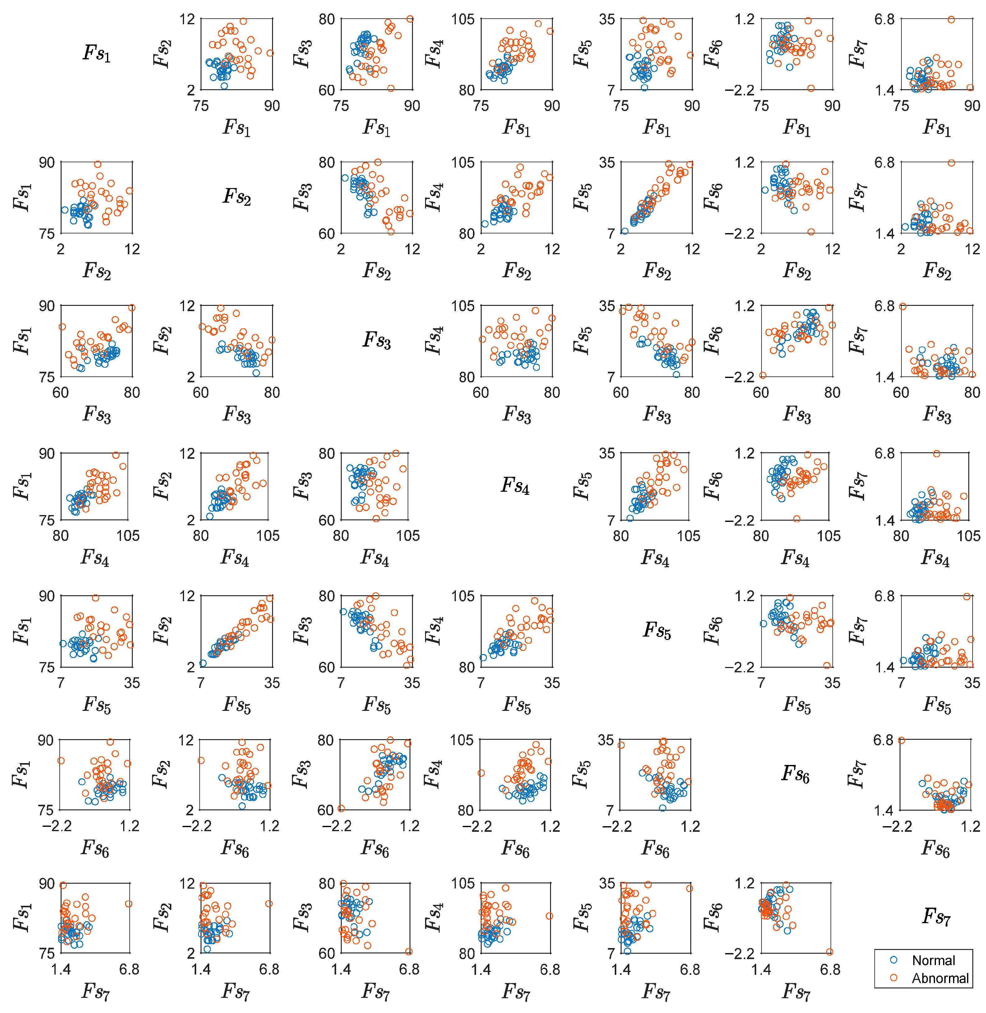
As described in Section 4.1, time domain feature sets, Fl and Fs, are extracted from long and short window training datasets, Xl and Xs, respectively. Here, Fl = {Flj | j = 1, …, 7} and Fs = {Fsj | j = 1, …, 7}. Fl1 = Fs1 = Average, Fl2 = Fs2 = Standard Deviation, Fl3 = Fs3 = Minimum Value, Fl4 = Fs4 = Maximum Value, Fl5 = Fs5 = Range, Fl6 = Fs6 = Skewness, and Fl7 = Fs7 = Kurtosis. Figure 6 and Figure 7 show the pairwise scatter plots among the extracted features Flj and Fsj, using blue- and orange-colored markers for normal and abnormal patterns underlying Xl and Xs, respectively.
As seen in Figure 6, the pairwise plots among Fl2, …, Fl5 distinctly classify the patterns for Xl, compared to the other pairs. This suggests that Fl2, …, Fl5 are important features for pattern recognition as long as a long window is considered. On the other hand, as seen in Figure 7, no pairwise plot distinctly classifies the patterns for Xs. Most of the pairs exhibit outliers and overlapping. Figure 7 also shows that some of the pairs among Fs1, …, Fs6 might be useful for classifying the patterns even though the features overlap. For instance, see the plots between Fs1 and Fs2, Fs5 and Fs2, Fs1 and Fs4, and Fs2 and Fs4. The above findings suggest that identifying important features from pairwise scatter plots is a cumbersome task, especially when the window is short.
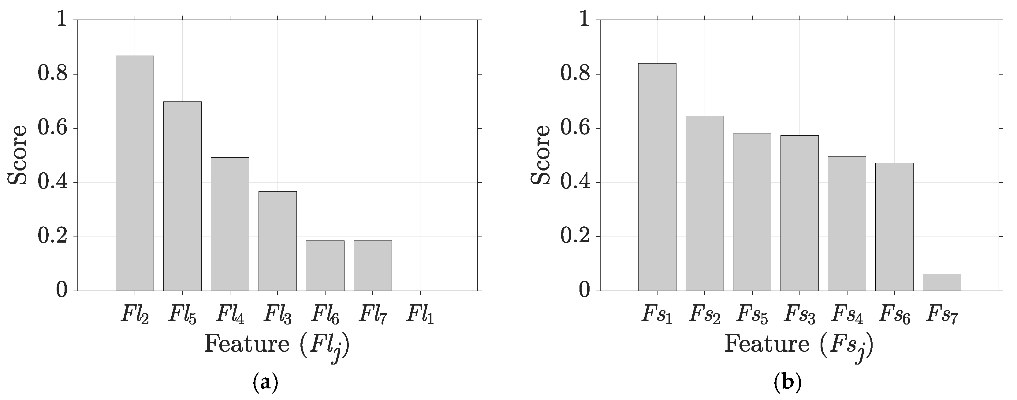
Nevertheless, as described in Section 4.1, the importance of features underlying the above Fl and Fs (see Figure 6 and Figure 7) are quantified for easing the feature selection process. For this, a MATLAB®-based RF algorithm is used. Figure 8a,b show the corresponding results, respectively.
As seen in Figure 8a, the RF algorithm ranks the Fl1, …, Fl7 in the following order: Fl2 > Fl5 > Fl4 > Fl3 > Fl6 > Fl7 > Fl1. Figure 8a also shows that the ranking scores are distinct. This means that there is no ambiguity regarding the importance of features. The importance can easily be categorized as follows. Fl2 and Fl5 are highly important, Fl4 and Fl3 are important, Fl6 and Fl7 are less important, and Fl1 is not important. These findings from Figure 8a resonate with the observation made from Figure 6.
As seen in Figure 8b, the RF algorithm ranks the Fs1, …, Fs7 in the following order: Fs1 > Fs2 > Fs5 > Fs3 > Fs4 > Fs6 > Fs7. Although the features are ranked, Figure 8b shows that the ranking scores are not distinct. In particular, the scores related to Fs2, Fs5, Fs3, Fs4, and Fs6, are close to each other, and thus the importance is ambiguous. These findings from Figure 8b resonate with the observation made from Figure 7.
However, as described in Section 4.1, the above outcomes (feature importance scores, see Figure 8a,b) result in sets of selected features, Fltrain and Fstrain, from Fl and Fs, respectively. As such, Fltrain = {Fl2, Fl5, Fl4, Fl3} and Fstrain = {Fs1, Fs2, Fs5, Fs3, Fs4, Fs6}, excluding less important and not important features as shown in Figure 8.
As described in Section 4.1, the above selected features, Fltrain and Fstrain, are then used for training a pattern recognition ANN, generating two trained models: ANN1, and ANN2, corresponding to long and short windows, respectively. The performance of the models is then tested using corresponding test datasets (Yl and Ys, respectively). Figure 9 and Figure 10 show the related results in the form of confusion matrixes, respectively.
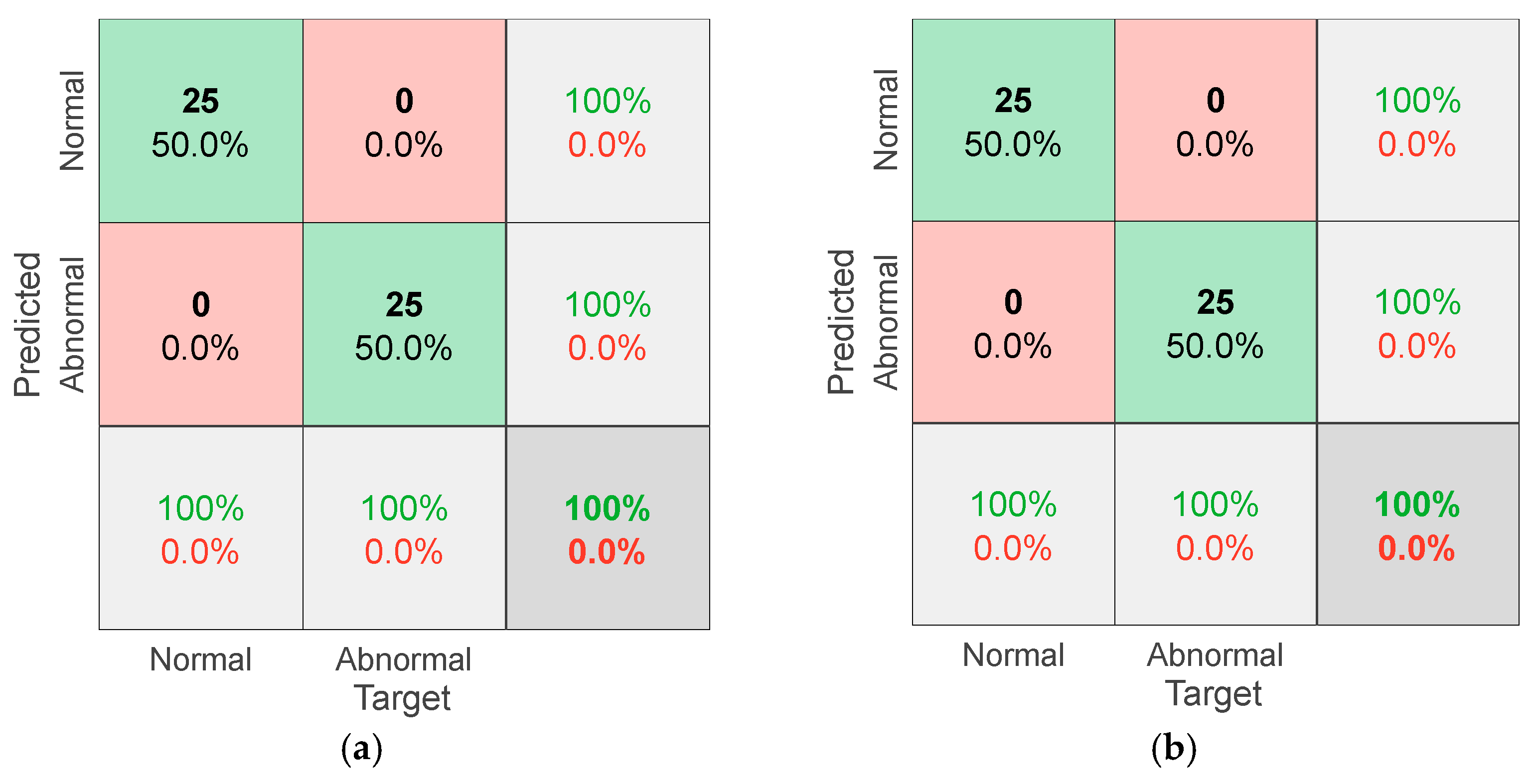
As seen in Figure 9, the ANN1 performs no mistake in pattern recognition. ANN1 predicts all the patterns (either normal or abnormal) correctly in both the training (see Figure 9a) and testing (see Figure 9b) phases. This implies that a feature-based ANN performs well when a long window is considered.
As seen in Figure 10, the accuracy of ANN2 in training phase is 94% (see Figure 10a). On the other hand, the accuracy of ANN2 in testing phase is 84% (see Figure 10b). As seen in Figure 10a, in training phase, ANN2 mistakenly predicts two (2) normal patterns as abnormal and one (1) abnormal pattern as normal. As seen in Figure 10b, in testing phase, ANN2 mistakenly predicts eight (8) normal patterns as abnormal. This implies that performance of a feature-based ANN drops when a short window is considered, especially in testing phase when the model is subjected to unseen data. This performance drop is obvious because of poorer feature resolution due to a short window, compared to that of a long window, as discussed above (see Figure 6, Figure 7 and Figure 8). Figure 10 also shows a large accuracy gap of 10% between the training and testing phases. It is worth mentioning that pertaining to a large gap, where accuracy in training is higher compared to that of testing, implies potential overfitting and generalization inability to respond to unseen data. Hence, it can be said that regardless of accuracy, the stability of a feature-based ANN also becomes questionable when a short window is considered.

5.2. Results for Non-Traditional Approach

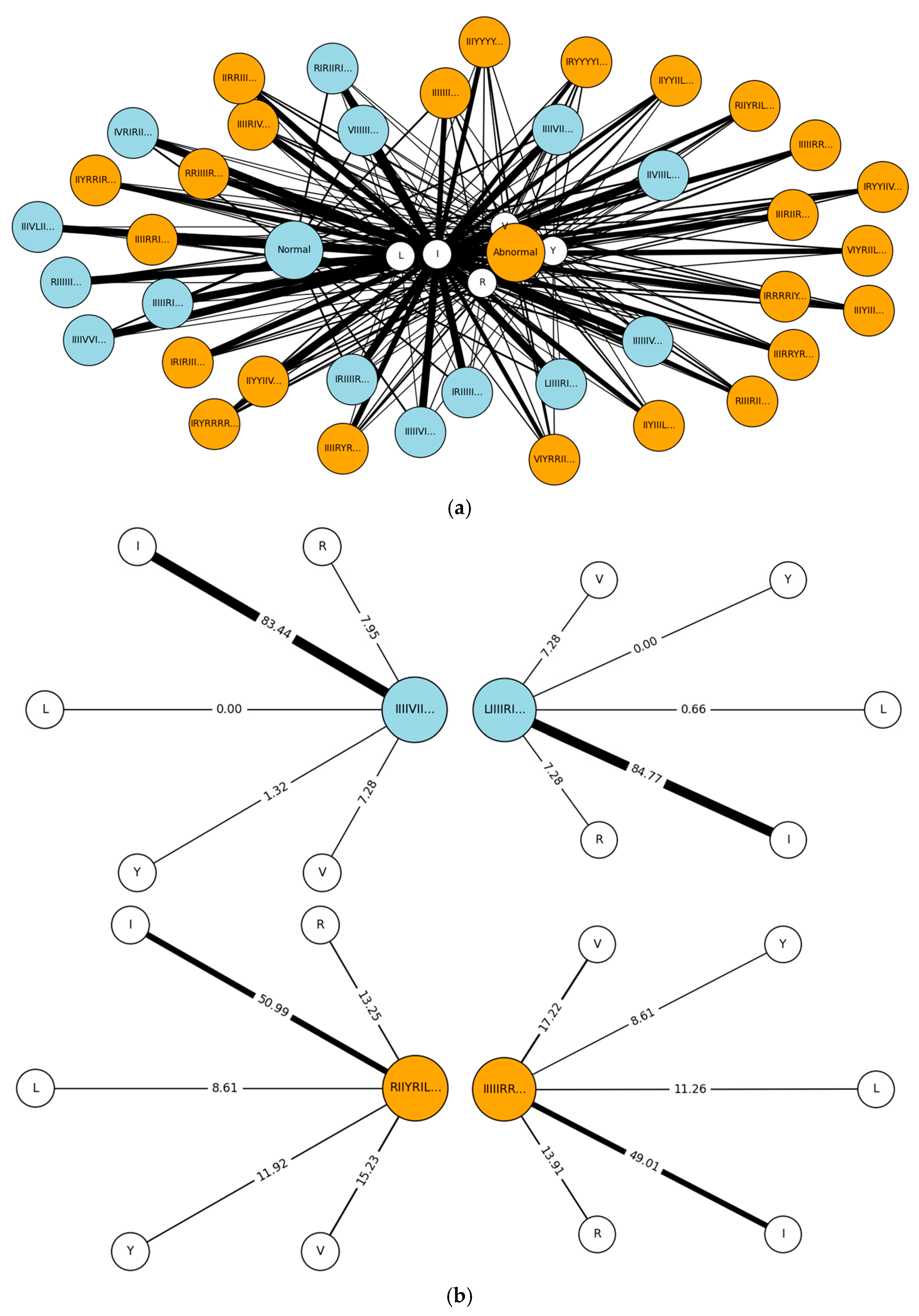
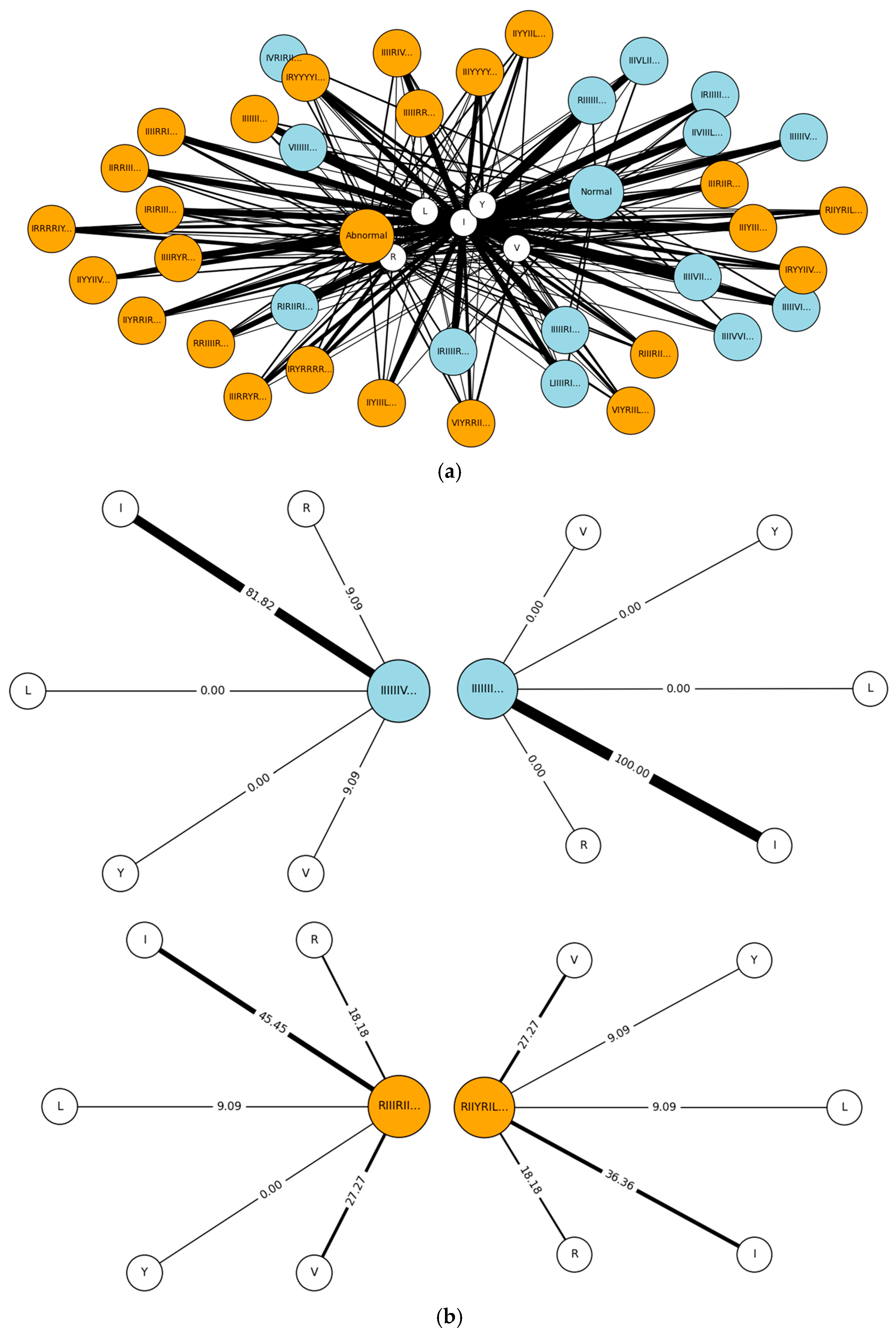
As described in Section 4.2, long and short window training datasets (Xl and Xs, respectively) are processed using a type-2 DBC, resulting in protein arrays. Consequently, the relative frequencies (RF in percentage (%)) of the array constituents are also calculated. As such, Figure 11 and Figure 12 show the related results for Xl and Xs, respectively, networking the interplay between the arrays and their constituents in a protein-verse.
As seen in Figure 11a, the blue- and orange-colored nodes represent protein arrays generated from normal and abnormal datasets underlying Xl, respectively. The white-colored nodes represent the array constituents (here, I, L, V, R, and Y) in all arrays. The connecting edges (black-colored lines) represent the relation between an array and its constituents in terms of RF. A thick edge represents high RF of a constituent compared to that of a thin edge for an array. For better understanding, Figure 11b shows four instances (two instances for normal and two for abnormal) underlying the network shown in Figure 11a.
As seen in Figure 11b, a protein array subjected to a normal pattern (blue-colored nodes) shows high RF of the constituent ‘I’ compared to that of other constituents (L, V, R, and Y). The RF for L, V, R, and Y are very low and even sometimes zero (0). A zero (0) RF indicates the absence of a constituent in an array. On the other hand, as seen in Figure 11b, a protein array subjected to an abnormal pattern (orange-colored nodes) shows a significant drop in the RF of ‘I’ compared to that of a normal pattern. Consequently, RF for L, V, R, and Y significantly increases compared to that of a normal pattern.
Similarly, as seen in Figure 12a, the blue- and orange-colored nodes represent protein arrays generated from normal and abnormal datasets underlying Xs, respectively. The white-colored nodes represent the array constituents (here, I, L, V, R, and Y) in all arrays. The connecting edges (black-colored lines) represent the relation between an array and its constituents in terms of RF. A thick edge represents high RF of a constituent compared to that of a thin edge for an array. For better understanding, Figure 12b shows four instances (two instances for normal and two for abnormal) underlying the network shown in Figure 12a.
As seen in Figure 12b, a protein array subjected to a normal pattern (blue-colored nodes) shows high RF of the constituent ‘I’ compared to that of other constituents (L, V, R, and Y). The RF for L, V, R, and Y are very low and even sometimes zero (0). A zero (0) RF indicates the absence of a constituent in an array. On the other hand, as seen in Figure 12b, a protein array subjected to an abnormal pattern (orange-colored nodes) shows a significant drop in the RF of ‘I’ compared to that of a normal pattern. Consequently, RF for L, V, R, and Y significantly increases, especially for V and R, compared to that of a normal pattern.
The above results (see Figure 11 and Figure 12) imply that the protein arrays retain the information content regardless of window size. In the case of a normal pattern, the RF of ‘I’ is high compared to that of other constituents, whether the window is long or short. On the other hand, in the case of an abnormal pattern, the RF of ‘I’ drops down, and the RF of other constituents increases significantly, whether the window is long or short.
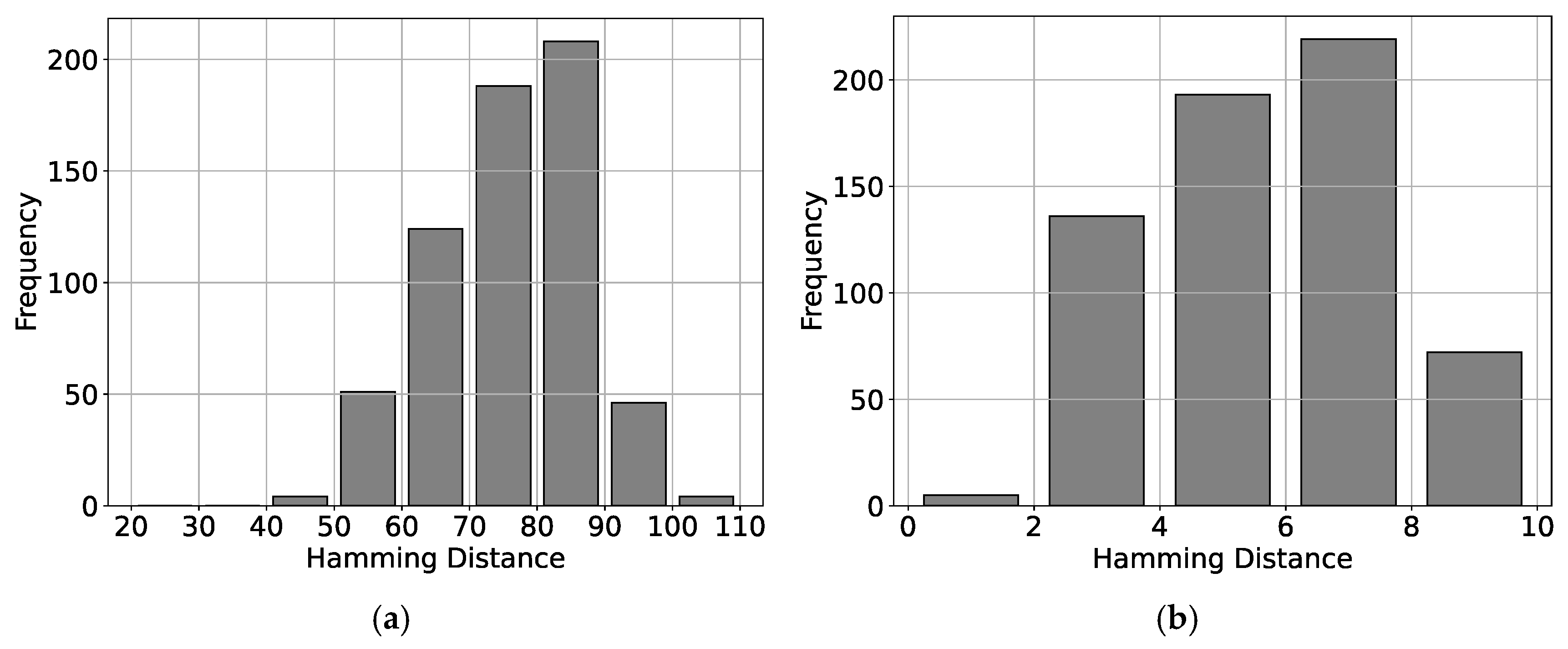
In addition to the constituents’ RF, another way to understand the dynamics underlying the arrays is to quantify the dissimilarity between normal and abnormal arrays. For this, one straightforward way is to measure hamming distance [46]. Here, hamming distance refers to the number of positions at which corresponding constituents between two arrays are different. For instance, say, ‘IIIIVIIIIIV’ and ‘IRYRRRRIIII’ are protein arrays for normal and abnormal patterns, respectively. The corresponding constituents differ at seven (7) positions (see the underlined positions), as follows: ‘IIIIVIIIIIV’ and ‘IRYRRRRIIII.’ Hence, the hamming distance between these arrays is seven (7). A high hamming distance indicates high dissimilarity. As such, the hamming distance between normal and abnormal arrays for both long and short windows (see Figure 11a and Figure 12a, respectively) are measured to understand the associated dissimilarity. Figure 13a,b show the corresponding results.
As seen in Figure 13a, when the window is long, the hamming distances are mostly in the range of 70 to 90. As seen in Figure 13b, when the window is short, the hamming distances are mostly in the range of 4 to 8. As such, the distances are appreciably high for both windows, indicating that associated dissimilarity is also high. These results further imply that the protein arrays obtained from the type-2 DBC are highly informative for understanding underlying patterns regardless of the window sizes.
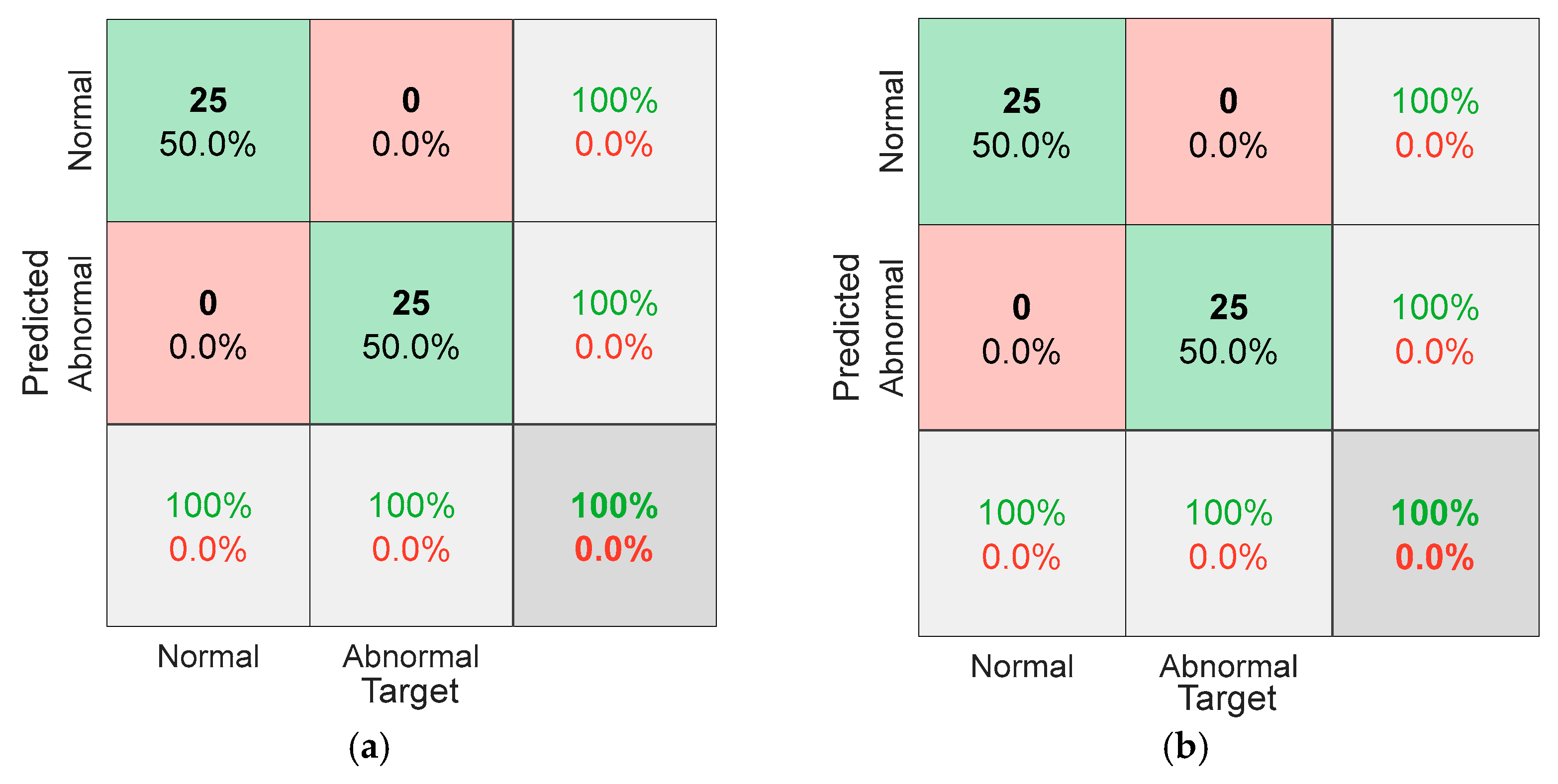
Nevertheless, as described in Section 4.2, the above RF is used for training a pattern recognition ANN, generating two trained models: ANN3, and ANN4, corresponding to long and short windows, respectively. The performance of the models is then tested using corresponding test datasets (Yl and Ys, respectively). Figure 14 and Figure 15 show the related results in the form of confusion matrixes, respectively.
As seen in Figure 14, the ANN3 performs no mistake in pattern recognition. ANN3 predicts all the patterns (either normal or abnormal) correctly in both the training (see Figure 14a) and testing (see Figure 14b) phases. This implies that a DBC-based ANN performs well when a long window is considered.
As seen in Figure 15, the accuracy of ANN4 in training phase is 86% (see Figure 15a). On the other hand, the accuracy of ANN4 in testing phase is 92% (see Figure 15b). As seen in Figure 15a, in training phase, ANN4 mistakenly predicts three (3) normal patterns as abnormal and four (4) abnormal patterns as normal. As seen in Figure 15b, in testing phase, ANN4 mistakenly predicts two (2) normal patterns as abnormal and two (2) abnormal patterns as normal. Figure 15 also shows a minimal accuracy gap of 6% between the training and testing phases. It is worth mentioning that pertaining to a minimal gap, where accuracy in testing is higher compared to that of training, implies good generalization ability to respond to unseen data.
Comparing the above results obtained for feature-based ANNs (see Figure 9 and Figure 10) and DBC-based ANNs (see Figure 14 and Figure 15), the ANNs, either feature-based or DBC-based, perform well when the window is long. Their performance falls when the window is short. In the case of a short window, the DBC-based ANN performs better than the feature-based ANN in recognizing patterns, exhibiting good generalization ability to respond to unseen data.
However, regarding the short window, cross-validating the performance of the above approaches (feature-based and DBC-based ANNs) is essential to understand how they perform for different dataset splits. For this, both approaches undergo a 20-fold Monte Carlo Cross-Validation (MCCV) [47]. In particular, 20 stratified training and test dataset splits (50:50) are generated randomly from Z (see Section 3, Figure 2) and then short-windowed. The short-windowed data for each split then undergoes the above approaches. Figure 16 and Figure 17 show the corresponding results.
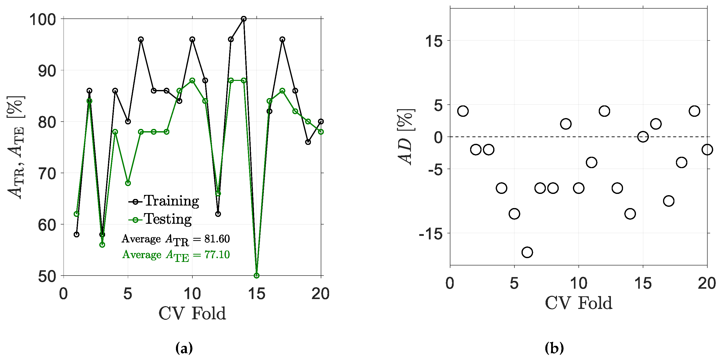
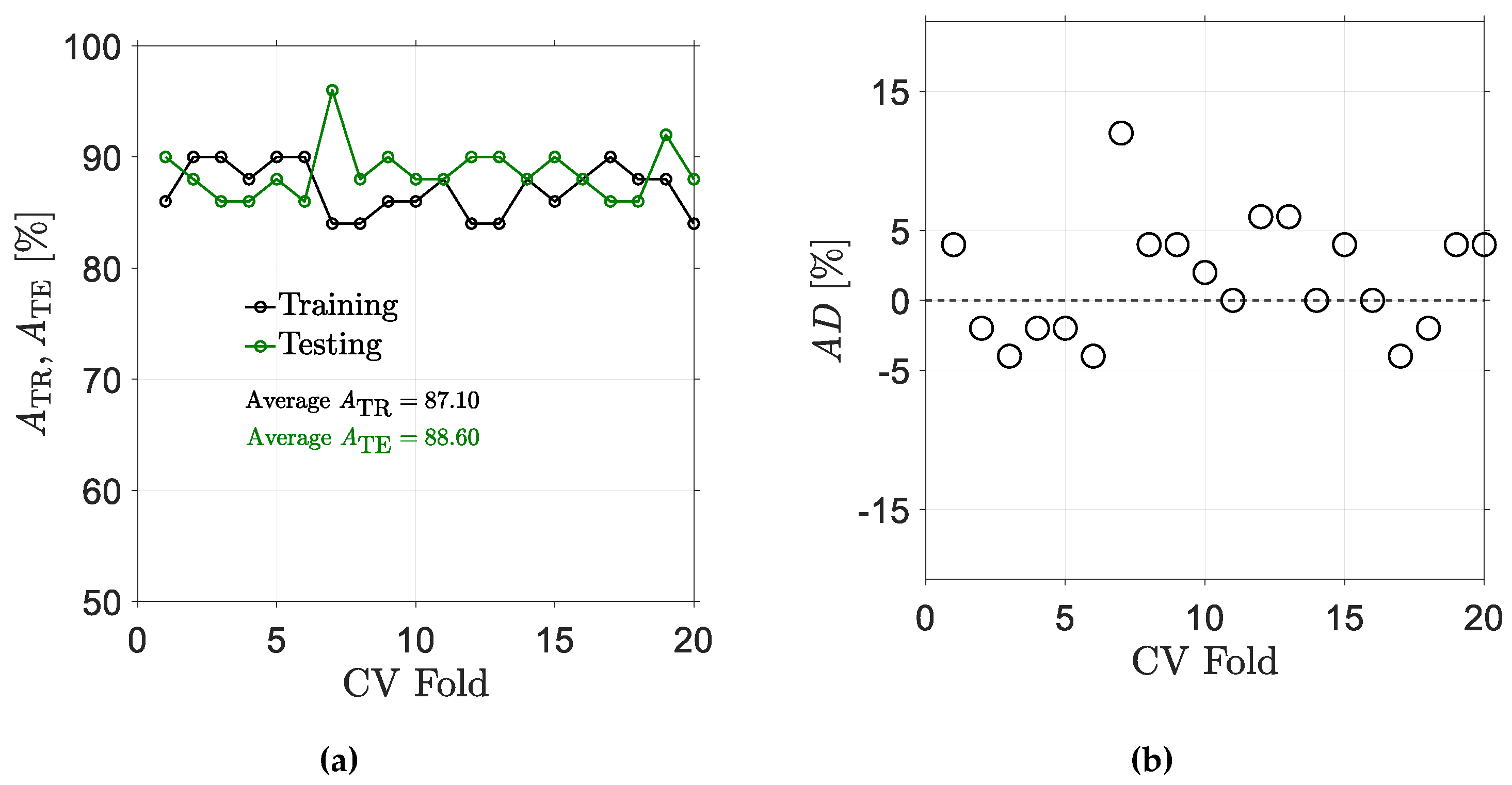
Regarding MCCV results for feature-based approach, Figure 16a shows the accuracy of the ANN in training (black-colored plot) and testing (green-colored plot) phases for 20 CV folds. Let the accuracy in training and testing phases be denoted as ATR and ATE, respectively. Let the accuracy difference between ATR and ATE be denoted as AD, such as AD = ATEATR. Figure 16b shows the AD for the same folds. Similarly, regarding MCCV results for DBC-based approach, Figure 17a shows the ATR (black-colored plot) and ATE (green-colored plot) for 20 CV folds. Figure 17b shows the AD for the same folds.
Figure 16a shows that ATR and ATE across CV folds exhibit instability. That said, the average accuracies for ATR and ATE are 81.60% and 77.10%, respectively. As seen in Figure 16b, almost half of the AD across CV folds are out of the range of [−5,5] %, and all of those are negative (<−5%). This implies that AD is often high, and when so, ATR is higher than ATE, indicating potential overfitting scenarios. As seen in Figure 16b, the rest of the AD across CV folds are within the range of [−5,5] %. When so, almost half of that exhibit very low ATR and ATE, and the rest exhibit considerably high ATR and ATE. For instance, consider fold no. 3 in Figure 16b. For fold no. 3, AD is −2. However, the corresponding ATR and ATE in Figure 16a are 58% and 56%, respectively. Similarly, consider fold no. 2 in Figure 16b. For fold no. 2, AD is −2. However, the corresponding ATR and ATE in Figure 16a are 86% and 84%, respectively. This implies that even when AD is minimal, it does not always guarantee a well-performed ANN.
On the other hand, regarding MCCV results for DBC-based approach, Figure 17a shows that ATR and ATE across CV folds exhibit stability. That said, the average accuracies for ATR and ATE are 87.10% and 88.60%, respectively. As seen in Figure 17b, almost all the AD across CV folds is within the range of [−5,5] %. Only three (3) are out of the range of [−5,5] %, and among those only one is very high and the other two are close to the range, i.e., 6%. This implies that AD is often minimal, indicating good generalization ability of the ANNs. This also implies that across different folds, a DBC-based ANN performs better compared to that of a feature-based ANN when window is short.

6. Concluding Remarks

Bioinspired computing methods, such as ANNs and their derivatives, are widely used in smart manufacturing (Industry 4.0/5.0) to support cognitive tasks like monitoring, prediction, and decision-making. A review of related works shows that these methods perform well when an appreciable amount of data is available. The methods fall short when few data are available. As such, there is a need for methods that can effectively handle smaller datasets or shorter windows, particularly in environments where rapid recognition and immediate corrective actions are crucial. This study sheds some light on this issue, focusing on the performance of a pattern recognition ANN under the constraints of shorter data windows (as few as 10 data points). Given the associated challenges, another bioinspired method, DNA-Based Computing (DBC), is introduced alongside the ANN to assess its effectiveness.
In particular, this study considers two types of datasets: long-window time series with approximately 150 data points and short-window time series with approximately 10 data points. Each dataset represents either a Normal or an Abnormal pattern and is processed using two approaches: feature-based ANN and DBC-based ANN. In the feature-based ANN approach, time-domain statistical features are extracted and used to train ANNs. In the DBC-based ANN approach, protein arrays derived from DBC are used instead. The results demonstrate that both approaches perform well in recognizing Normal and Abnormal patterns when long windows are available. However, with short windows, the feature-based ANN’s performance drops. In contrast, the DBC-based ANN performs better. These findings are further cross-validated through a 20-fold MCCV.
Overall, the findings of this study suggest that integrating DBC with ANN can significantly improve performance under extreme data-scarce conditions compared to traditional feature-based approaches. Beyond performance robustness, the findings also have broader implications for real-world manufacturing environments, where data scarcity often arises not only from short windowing but also from issues such as signal delays, packet loss, or fragmentation in distributed sensor networks [13,14,48,49]. The demonstrated ability of DBC to extract meaningful information from limited data highlights its potential effectiveness under these constraints. Moreover, the capacity to operate reliably with fewer data points may reduce the need for high-frequency sampling, thereby extending sensor lifetime, lowering storage demands, and improving energy efficiency [14,50,51]. These advantages are particularly relevant in the context of ongoing digital (DX) and green (GX) transformations in modern manufacturing [52,53,54]. Future research will focus on systematically expanding these directions. As such, by offering a viable strategy for handling extreme data-scarce conditions, this study contributes to the development of adaptive, resource-efficient, and resilient futuristic manufacturing systems.

Author Contributions

Conceptualization, A.K.G. and S.U.; methodology, A.K.G. and S.U.; software, A.K.G.; validation, A.K.G. and S.U.; formal analysis, A.K.G.; investigation, A.K.G.; resources, S.U.; data curation, A.K.G. and S.U.; writing—original draft preparation, A.K.G.; writing—review and editing, A.K.G. and S.U.; visualization, A.K.G. and S.U.; supervision, S.U.; project administration, S.U.; funding acquisition, S.U. All authors have read and agreed to the published version of the manuscript.

Funding

This research received no external funding.

Data Availability Statement

The datasets used in this study are available from the following URL: https://github.com/commons-repo/001-research-data.git (accessed on 20 August 2025). One may also access them via the GitHub CLI (command line interface) using the command: gh repo clone commons-repo/001-research-data.

Conflicts of Interest

The authors declare no conflicts of interest.

Appendix A. Glossary of Symbols Related to Section 3 and Section 4

Table A1. Section 3 and Section 4-related symbols and their meaning.
SymbolsMeaningSections
ZSet of all generated datasets (100 total, 50 Normal and 50 Abnormal).3
ZkThe k-th dataset in Z, where k = 1, …, 100.3
Zk(i)The i-th point in dataset Zk, where i = 0, …, N and N is the window size.3
X, YSets of training and test datasets, respectively.
Mutually exclusive subsets of Z, each containing 50 Normal/Abnormal datasets.
3
Nl, NsLong window size (=150) and short window size (=10), respectively.3
Xl, XsLong and short window training datasets, respectively.3, 4
Yl, YsLong and short window test datasets, respectively.3, 4
Fl, FsSets of extracted time-domain features from Xl and Xs, respectively.4
Flj, FsjIndividual features where j = 1, …, 7.
Fl1 = Fs1 = Average,
Fl2 = Fs2 = Standard Deviation,
Fl3 = Fs3 = Minimum Value,
Fl4 = Fs4 = Maximum Value,
Fl5 = Fs5 = Range,
Fl6 = Fs6 = Skewness, and
Fl7 = Fs7 = Kurtosis
4
Fltrain, FstrainSelected subsets of Fl and Fs, respectively, after feature selection process.4
Fltest, FstestExtracted features from Yl and Ys, respectively, corresponding to Fltrain and Fstrain.4
ANN1, ANN2, ANN3, ANN4ANN models trained on different inputs.
ANN1 is trained on Fltrain,
ANN2 is trained on Fstrain,
ANN3 is trained on RFXl, and
ANN4 is trained on RFXs.
4
Dok(i)Time series dataset element, where D ∈ {X, Y}, o ∈ {l, s}, k = {1, …, 100}, i = {0, …, No}.4
r1, r2, r3DNA-forming rules applied to Dok(i).4
DNAm(Dok(i))DNA array element derived from Dok(i) under rule rm (m = 1,2,3).4
DNAm(Dok)DNA array of dataset Dok, generated using the rule rm (m = 1,2,3).4
mRNADok(i)Codon (3-letter mRNA symbol) formed from DNA arrays.4
ProteinDok(i)Protein symbol (1-letter amino acid) derived from codon mRNADok(i).4
ProteinDokSequence (array) of protein symbols for dataset Dok.4
gGenetic rules mapping codons to amino acids.4
PSet of all possible amino acids encoded in a protein array.4
pA particular amino acid in P.4
CpNumber of times amino acid p appears in P.4
CTotal number of proteins in P.4
RF(p)Relative frequency of amino acid p, defined as Cp/C.4
RFDokSet of relative frequencies for dataset Dok.4
RFDoAggregated set of relative frequencies for datasets under condition o.4
RFXl, RFXsSets of DBC-driven features for long- and short-windowed training datasets, respectively.4
RFYl, RFYsSets of DBC-driven features for long- and short-windowed test datasets, respectively.4

Appendix B. Pseudocode for the Feature Extraction Process

Table A2. Pseudocode for the feature extraction process.
StepsDescription
Step 1START
Step 2Specify the input folder path containing text (*.txt) files of the datasets.
Step 3Enumerate all files matching ‘*.txt’ in the folder.
Step 4Initialize empty containers for each output column:
patternTypes, datasetIDs, F1, …, F7.
Step 5FOR each file in the list:
 5.1 Open file for reading.
 5.2 Read Line 1; parse substring after ‘Pattern Type:’ → ‘ptype’.
 5.3 Read Line 2; parse integer after ‘Dataset ID:’ → ‘id’.
 5.4 Read ‘numeric data’ from Line 3 to end into vector ‘x’.
 5.5 Compute:
   F1 ← average (x),
   F2 ← standard deviation (x),
   F3 ← min (x),
   F4 ← max (x),
   F5 ← range (x),
   F6 ← skewness (x), and
   F7 ← kurtosis (x).
 5.6 Append records (ptype, id, F1, …, F7) to outputs (patternTypes,
    datasetIDs, F1, …, F7).
 5.7 Close file.
END FOR
Step 6Assemble all records into a table in the column order specified in Step 4.
Step 7Write the table to ‘Features.csv’ in the same folder mentioned in Step 1.
Step 8END
Table A3. The Minimal MATLAB® (version: R2024b) code skeleton corresponding to Table A2.
Code
% Configure paths
folderPath = ‘INPUT_FOLDER_PATH’; % e.g., ‘C:\path\to\data’
outCSV = ‘OUTPUT_CSV_NAME.csv’; % e.g., ‘Features.csv’

% Enumerate files
files = dir(fullfile(folderPath, ‘*.txt’));
n = numel(files);

% Preallocate containers
patternTypes = strings(n,1);
datasetIDs = zeros(n,1);
F1 = zeros(n,1); F2 = zeros(n,1); F3 = zeros(n,1); F4 = zeros(n,1);
F5 = zeros(n,1); F6 = zeros(n,1); F7 = zeros(n,1);

% Process each file
for i = 1:n
  fp = fullfile(files(i).folder, files(i).name);
  % Read header lines
  fid = fopen(fp, ‘r’);
  line1 = fgetl(fid); % “Pattern Type: <label>”
  line2 = fgetl(fid); % “Dataset ID: <int>”
  fclose(fid);
  % Parse header values
  patternTypes(i) = strtrim(erase(line1, ‘Pattern Type:’));
  datasetIDs(i) = sscanf(line2, ‘Dataset ID: %d’);
  % Read numeric data from line 3 onward
  x = readmatrix(fp, ‘NumHeaderLines’, 2);
  x = x(:);
  % Compute features
  F1(i) = mean(x); % Average
  F2(i) = std(x); % Standard Deviation
  F3(i) = min(x); % Minimum
  F4(i) = max(x); % Maximum
  F5(i) = F4(i)–F3(i); % Range
  F6(i) = skewness(x); % Skewness
  F7(i) = kurtosis(x); % Kurtosis
end

% Assemble table in the exact column order
T = table(patternTypes, datasetIDs, F1, F2, F3, F4, F5, F6, F7, ‘VariableNames’, {‘PatternType’, ‘DatasetID’, ‘F1’, ‘F2’, ‘F3’, ‘F4’, ‘F5’, ‘F6’, ‘F7’});

% Write CSV
writetable(T, fullfile(folderPath, outCSV));

Appendix C. Pseudocode for the Feature Selection Process

Table A4. Pseudocode for the feature selection process.
StepsDescription
Step 1START
Step 2Get features and class labels:
 2.1 Input features and pattern type for datasets (e.g., from the file ‘Features.csv’ created in Appendix B).
 2.2 Select feature columns (e.g., features listed in the ‘F1, …, F7’ columns in ‘Features.csv’) as predictors.
 2.3 Select pattern types (e.g., Normal/Abnormal patterns listed in the ‘PatternType’ column in ‘Features.csv’) as class labels.
Step 3Convert class labels to categorical (if needed).
Step 4Run MATLAB®-based Random Forest Classifier (TreeBagger):
 4.1 Set random seed for reproducibility.
 4.2 Set number of trees (e.g., 30).
 4.3 Train classifier with OOB prediction and permutation importance enabled, keeping other
parameters at MATLAB® defaults.
Step 5Display feature importance:
 5.1 Obtain permutation importance scores.
 5.2 Sort scores descending and reorder feature names accordingly.
 5.3 Plot feature importance scores as a bar chart.
 5.4 Print feature importance scores.
Step 6END.
Table A5. The Minimal MATLAB® (version: R2024b) code skeleton corresponding to Table A4.
Code
% Getting features and the class label
% Input features and pattern type; e.g., ‘Features.csv’ from Appendix B)
TrainingFeatures = readtable(‘INPUT_FEATURES_PATH.csv’); % e.g., ‘C:\path\to\Features.csv’
featuresRF = TrainingFeatures(:, 3:end); % Select predictors F1–F7
classLabelsRF = TrainingFeatures.PatternType; % Use PatternType as class label

% Convert class labels to categorical if they aren’t already
classLabelsRF = categorical(classLabelsRF);

% Random forest classifier
rng(1); % Set random seed for reproducibility
numTrees = 30; % Number of trees
model = TreeBagger(numTrees, featuresRF, classLabelsRF, ‘Method’, ‘classification’, ‘OOBPrediction’, ‘On’, ‘OOBVarImp’, ‘On’);

% Display feature importance
featureImportance = model.OOBPermutedVarDeltaError;
[sortedImportance, sortedIndices] = sort(featureImportance, ‘descend’);
sortedFeatures = featuresRF.Properties.VariableNames(sortedIndices);

% Plot feature importance
figure;
bar(sortedImportance);

% Customize plot
xlabel(‘Feature’, ‘FontSize’, 24);
ylabel(‘Score’, ‘FontSize’, 24);
set(gca, ‘XTick’, 1:numel(sortedFeatures), ‘XTickLabel’, sortedFeatures, ‘XTickLabelRotation’, 0, ‘TickLabelInterpreter’, ‘none’);
set(gca, ‘XGrid’, ‘on’, ‘YGrid’, ‘on’);
set(gca, ‘TickDir’, ‘out’);
set(gca, ‘Box’, ‘on’);
grid on;

% Print out the names and importance scores of the features
disp(‘Features by importance:’);
disp(table(sortedFeatures(:), sortedImportance(:), ‘VariableNames’, {‘Feature’, ‘Score’}));
For further details and examples of MATLAB®’s TreeBagger function, see the official documentation available at https://www.mathworks.com/help/stats/treebagger.html (accessed on 20 August 2025).

Appendix D. Pseudocode for the Machine Learning

Table A6. Pseudocode for the Machine Learning.
StepsDescription
Step 1START
Step 2Prepare training data:
 2.1 Load the table of selected features and one-hot labels for training.
 2.2 Define inputs as all selected feature columns.
 2.3 Define targets as the final two one-hot columns (one-hot: Normal, Abnormal).
 2.4 Convert inputs and targets to numeric arrays and transpose so columns represent samples, as required by MATLAB®.
Step 3Define and train ANN:
 3.1 Create a pattern recognition feed-forward network.
 3.2 Train the network on training inputs and targets.
Step 4Prepare test data:
 4.1 Load the table of selected features and one-hot labels for testing.
 4.2 Define test inputs as all selected feature columns.
 4.3 Define test targets as the final two one-hot columns (one-hot: Normal, Abnormal).
 4.4 Convert test inputs and targets to numeric arrays and transpose so columns represent samples, as required by MATLAB®.
Step 5Evaluate on test data:
 5.1 Compute outputs for the test inputs.
 5.2 Convert outputs to predicted class indices.
 5.3 Display predicted indices.
 5.4 Plot the confusion matrix using true one-hot targets vs. predicted outputs.
Step 6END.
Table A7. The Minimal MATLAB® (version: R2024b) code skeleton corresponding to Table A6.
Code
% Training data
% Load the table (selected features + one-hot labels from a csv file)
trainTbl = readtable(‘INPUT_SELECTED_FEATURES_TRAIN.csv’); % e.g., ‘C:\path\to\SelectedFeatures_Train.csv’

% Creating inputs and targets for training
% Assumes layout: [ … feature columns …, Normal, Abnormal ]
train_input = trainTbl(:, 2:end-2);
train_target = trainTbl(:, end-1:end); % two one-hot columns: [Normal, Abnormal]

% Convert table to array and transpose (columns = samples)
train_input = table2array(train_input)’;
train_target = table2array(train_target)’;

% Define & Train the ANN
% MATLAB®-based Two-layer feed-forward net for pattern recognition with 3 hidden neurons (number of hidden neurons can be configured if needed)
net = patternnet(3);

% Train the network
[net, tr] = train(net, train_input, train_target);

% Test data
% Load the table (selected features + one-hot labels from a csv file)
testTbl = readtable(‘INPUT_SELECTED_FEATURES_TEST.csv’); % e.g., ‘C:\path\to\SelectedFeatures_Test.csv’

% Creating inputs and targets for testing
test_input = testTbl(:, 2:end-2);
test_target_real = testTbl(:, end-1:end);

% Convert and transpose
test_input = table2array(test_input)’;
test_target_real = table2array(test_target_real)’;

% Inference & evaluation
% Network predictions (continuous outputs; each column sums ~1 due to softmax)
test_output_pred = net(test_input);
% Convert outputs to predicted class indices (1=Normal, 2=Abnormal if that order)
test_pred_idx = vec2ind(test_output_pred);

% Inspect predicted indices
disp(‘Predicted class indices:’);
disp(test_pred_idx);

% Confusion matrix plot (targets: one-hot; outputs: network predictions)
figure;
plotconfusion(test_target_real, test_output_pred);
title(‘Confusion Matrix’);
For further details and examples of MATLAB®’s pattern recognition neural net, see the official documentation available at https://www.mathworks.com/help/deeplearning/ref/patternnet.html (accessed on 20 August 2025).

Appendix E. The Central Dogma of Molecular Biology

The central dogma of molecular biology establishes the logical and physical relationships among macromolecules such as DNA, RNA, and proteins. In particular, biological systems only allow information flows such as “DNA to DNA,” “DNA to RNA,” and “RNA to protein” [23,45]. A comprehensive description of DNA–RNA–protein-centric processes can be found in [55]. In this article, the objective is to gain inspiration from the core processes of the central dogma and build models (algorithms) to solve cognitive problems (here, extracting features from short-windowed signal datasets). Therefore, a customized and concise description of the core processes underlying the central dogma of molecular biology is presented below.
Figure A1. Schematic illustration of the central dogma of molecular biology.
Make 07 00096 g0a1
The central dogma of molecular biology governs how genetic information flows within biological systems: from DNA to RNA to protein. As seen in Figure A1, this flow includes DNA replication (DNA to DNA), transcription (DNA to mRNA), and translation (mRNA to protein). Reverse transcription such as mRNA to DNA is also possible, but the reverse flow from protein to mRNA or DNA is fundamentally impossible.
DNA molecules consist of four elements (A, C, G, T); RNA molecules (e.g., mRNA) also consist of four elements (U, C, G, A); in contrast, proteins consist of twenty elements (20 types of amino-acids). As seen in Figure A1, DNA transcription and RNA translation are the two main processes involved in protein synthesis. During transcription, the elements of DNA, namely A, C, G, T, are transcribed to U, G, C, A, respectively, when an mRNA is formed. During translation, each of the three consecutive elements of mRNA is considered a codon, which corresponds to an amino-acid in a protein. These relationships ultimately establish a deterministic mapping between the three-letter codons composed of four DNA bases (A, C, G, and T) and the one-letter representations of twenty amino acids used in proteins (Alanine (A), Arginine (R), Asparagine (N), Aspartic acid (D), Cysteine (C), Glutamine (Q), Glutamic acid (E), Glycine (G), Histidine (H), Isoleucine (I), Leucine (L), Lysine (K), Methionine (M), Phenylalanine (F), Proline (P), Serine (S), Threonine (T), Tryptophan (W), Tyrosine (Y), and Valine (V)). The resulting codon-to-amino acid mapping constitutes the genetic rules—a universally conserved mechanism that governs protein synthesis across all biological organisms [23,30,48]. The 1-letter symbols of amino-acids in Figure A1 (M, T, L, S, R) correspond to the genetic rules. Table A8 outlines these rules as well. For instance, as outlined in Table A8, if a codon (denoted as C) belongs to the set {ATT, ATC, ATA}, then the corresponding amino acid (denoted as AA) is I.
Table A8. Genetic rules (Rearranged from [30]).
No.Genetic Rules (Codon = C, Amino Acid = AA)
1IF C ∈ {ATT, ATC, ATA} THEN AA = I
2IF C ∈ {CTT, CTC, CTA, CTG, TTA, TTG} THEN AA = L
3IF C ∈ {GTT, GTC, GTA, GTG} THEN AA = V
4IF C ∈ {TTT, TTC} THEN AA = F
5IF C ∈ {ATG} THEN AA = M
6IF C ∈ {TGT, TGC} THEN AA = C
7IF C ∈ {GCT, GCC, GCA, GCG} THEN AA = A
8IF C ∈ {GGT, GGC, GGA, GGG} THEN AA = G
9IF C ∈ {CCT, CCC, CCA, CCG} THEN AA = P
10IF C ∈ {ACT, ACC, ACA, ACG} THEN AA = T
11IF C ∈ {TCT, TCC, TCA, TCG, AGT, AGC} THEN AA = S
12IF C ∈ {TAT, TAC} THEN AA = Y
13IF C ∈ {TGG} THEN AA = W
14IF C ∈ {CAA, CAG} THEN AA = Q
15IF C ∈ {AAT, AAC} THEN AA = N
16IF C ∈ {CAT, CAC} THEN AA = H
17IF C ∈ {GAA, GAG} THEN AA = E
18IF C ∈ {GAT, GAC} THEN AA = D
19IF C ∈ {AAA, AAG} THEN AA = K
20IF C ∈ {CGT, CGC, CGA, CGG, AGA, AGG} THEN AA = R
21IF C ∈ {TAA, TAG, TGA} THEN AA = X
Note: For computational purposes, the three-letter DNA bases are considered codons. The amino acid denoted as X (or, None) does not exist (see rule no. 21), i.e., TAA, TAG, and TGA do not code any amino acids in physical sense. For computational purposes, TAA, TAG, or TGA is translated into X.
Since DNA/RNA are 4-element pieces of information and proteins are 20-element pieces of information, the central dogma of molecular biology eventually refers to creating many-element pieces of information (protein-type) from few-element pieces of information (DNA- and RNA-type). This metaphor forms the conceptual foundation of the DNA-Based Computing (DBC) framework [23]. DBC can be used to solve cognitive problems, based on pattern recognition, associated with smart manufacturing. Depending on the nature of the problem, different forms of DBC may be applied [30,32]. The version used in this study—suitable for sensor signal-based machine learning—corresponds to type-2 DBC [23,30], which is further detailed in Section 4.2 and Appendix F.

Appendix F. Type-2 DNA-Based Computing (DBC)
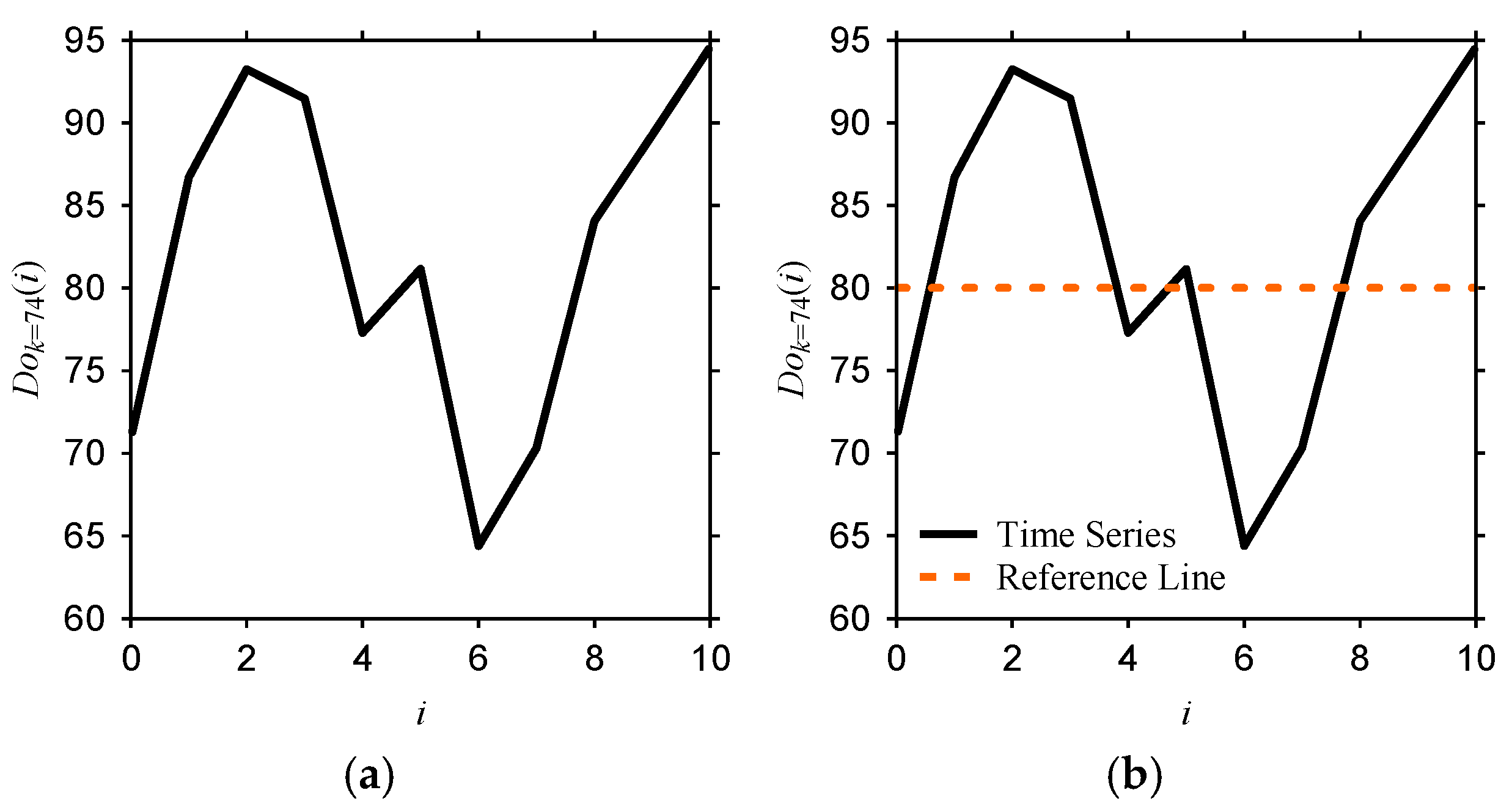
Consider a time series dataset denoted as Dok(i), as shown in Figure A2. Let R ∈ ℜ be a reference value. For instance, when R = 80, Figure A3 depicts its relative position within the dataset.
Thus, a new variable called Difference(Dok(i),R) is used to find the difference between Dok(i) and R. As such, the following relationship holds: Difference(Dok(i),R) = Dok(i) − R, i = 0, 1, …. The left-hand side of Figure A3 illustrates this outcome in graphical form, where the difference is plotted against the index i.
Figure A2. (a) Instance of a time series dataset and (b) Instance of (a) with a reference (= 80).
Make 07 00096 g0a2
Figure A3. Outlining the DNA-forming rule using in this study.
Make 07 00096 g0a3
The sequence of differences, i.e., Difference(Dok(i),R), i = 0, 1, …, is then represented by a symbolic sequence, analogous to a strand or array of natural DNA. Each element of this array belongs to {A,C,G,T}. This representation is obtained by applying the DNA-forming rule shown in the center of Figure A3. Say, the parameters related to this rule are set as: a = 12.5, b = 7.5, c = −7.5, and d = −12.5. The set parameters divide the difference plot into four regions corresponding to A, C, G, and T, as shown on the right-hand side of Figure A3. This way, each difference value is mapped to a DNA symbol, resulting in a complete symbolic DNA array.
Note that the DNA-forming rule is inherently flexible. The related parameters (a, b, c, and d), as well as the reference value (R), are user-defined and can be adjusted depending on the characteristics of the problem under study. In this way, different parameterizations may be applied across application contexts, rather than being restricted to a single fixed configuration. As such, users can explore and generate symbolic DNA strands or arrays from the time series. For example, keeping the same values of a, b, c, and d but altering the reference R produces multiple DNA arrays for the same dataset. This study adapts this approach, as described in [30]. Based on this rationale, the specific parameters associated with the DNA-forming rules employed in this study are summarized in Table A9.
Table A9. Parameters related to DNA-forming rules [30].
Rule 1 (r1)Rule 2 (r2)Rule 3 (r3)
Reference = 80
a = 12.5
b = 7.5
c = −7.5
d = −12.5
Reference = 100
a = 12.5
b = 7.5
c = −7.5
d = −12.5
Reference = 60
a = 12.5
b = 7.5
c = −7.5
d = −12.5
As seen in Table A9, this study adapts three DNA-forming rules, denoted as r1, r2, and r3 (also mentioned in Section 4.2). The parameters (a, b, c, d) remain the same for each rule, while the reference values differ (80, 100, and 60, respectively). Based on the DNA-forming rule creation criteria described above and illustrated in Figure A3, this leads to three distinct mapping schemes, similar to that shown in Figure A3. Consequently, three DNA arrays are generated for Dok, denoted as DNA1(Dok), DNA2(Dok), and DNA3(Dok), corresponding to r1, r2, and r3, respectively. The left-hand side of Figure A4 illustrates these DNA arrays explicitly.
Figure A4. Outlining the DNA-to-mRNA-to-Protein flow in type-2 DBC.
Make 07 00096 g0a4
As seen on the left-hand side of Figure A4, DNA1(Dok) = GATCAATGACT, DNA2(Dok) = TTAGTTTTTGA, and DNA3(Dok) = CTTTTTACTTT. The DNA arrays are then combined to generate an mRNA array by applying the mRNA-forming rule described in Section 4.2. In practice, this rule means appending the i-th element from each DNA array side by side. For example, the first element of DNA1, DNA2, and DNA3 are placed together, followed by the second element of each, and so on. This step-by-step concatenation produces a sequence of triplets (three-letter units), i.e., codons. As such, for the present dataset, the resulting codons and mRNA array are as follows. GTC ATT TAT CGT ATT ATT TTA GTC ATT CGT TAT = GTCATTTATCGTATTATTTTAGTCATTCGTTAT. The center part of Figure A4 illustrates this flow.
As seen on the right-hand side of Figure A4, each codon (three-letter triplet) in the mRNA array is then mapped to a one-letter amino acid symbol according to the genetic rules summarized in Appendix E (see Table A8). For example, in the present case, the first codon ‘GTC’ corresponds to rule number 3 in Table A8, which specifies the amino acid symbol ‘V (Valine)’. All the other codons are converted into their respective amino acid symbols, similarly. The outcome is a sequence of amino acid symbols, i.e., a protein array. Thus, for the present dataset, the resulting protein array is VIYRIILVIRY. This way, the time series dataset (denoted as Dok) is ultimately transformed into a protein array (denoted as ProteinDok).
Now, to convert this symbolic array (VIYRIILVIRY) into numerical features suitable for machine learning, the relative frequencies of the constituent amino acids are calculated, as described in Section 4.2. For instance, in this array of length 11, ‘I’ occurs 4 times, ‘V’ 2 times, ‘Y’ 2 times, ‘R’ 2 times, and ‘L’ once. Accordingly, as mentioned in Section 4.2, RF(I) = 4/11 ≈ 36.4%, RF(V) = 18.2%, RF(Y) = 18.2%, RF(R) = 18.2%, and RF(L) = 9%.
The abovementioned procedure is consistently applied to all (long/short-windowed normal/abnormal) datasets, thereby yielding quantitative features for the subsequent machine learning analyses presented in this study.
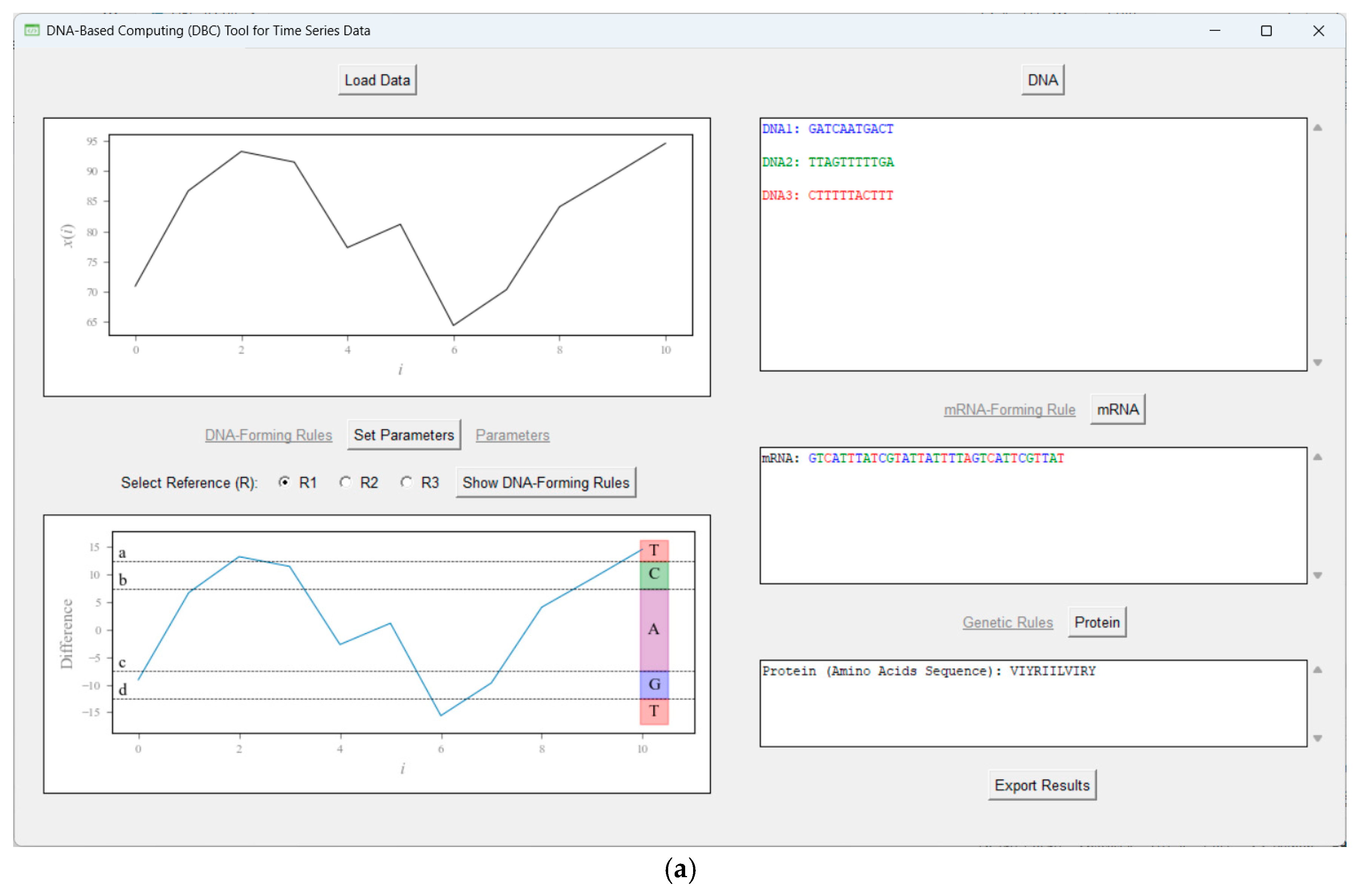
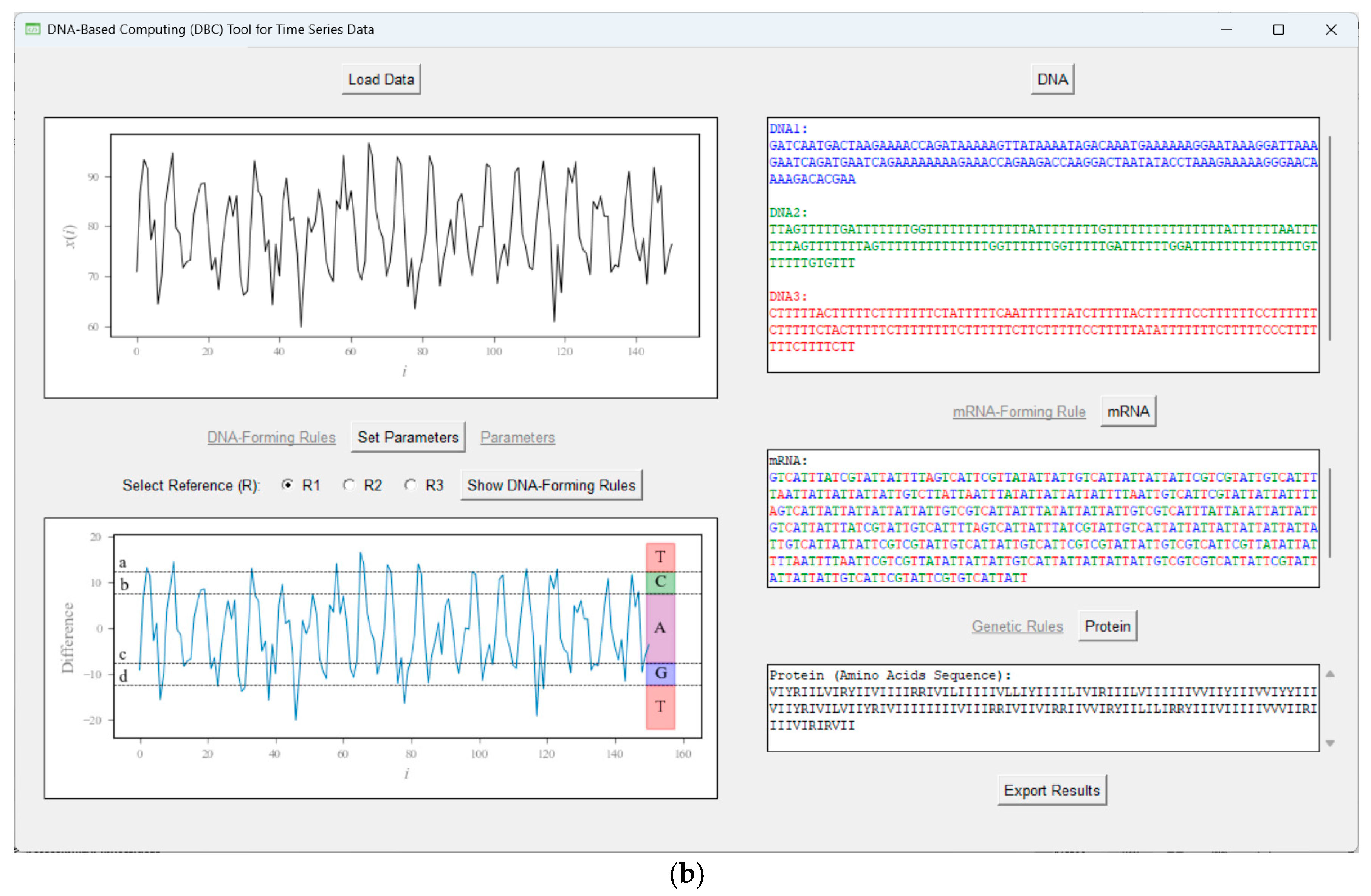
Nevertheless, a GUI-based tool has also been developed to perform the abovementioned type-2 DBC on time series datasets. Figure A5a shows a screenshot where a short-windowed dataset is converted into a protein array. Figure A5b shows a corresponding screen-print for the same dataset but with a long-window configuration, resulting in a different protein array. Note that this is the same dataset that is used to illustrate the stepwise process in Figure A2, Figure A3 and Figure A4, thereby providing consistency between the illustrative example and the tool-based implementation. These screen-print results follow the same DNA-forming, mRNA-forming, and genetic rules described above, ensuring methodological consistency. Notably, the tool also allows users to define their own DNA-forming parameters (a, b, c, d, and reference) through the interface (by selecting the ‘Set Parameters’ button). The source code for this tool is also made publicly available via the same GitHub repository mentioned in Section 3. One may access the repository using the URL: https://github.com/commons-repo/001-research-data.git (accessed on 20 August 2025). One may also access via the GitHub CLI (command line interface) using the command: gh repo clone commons-repo/001-research-data.
Figure A5. Screen-print of the DBC tool’s interface for (a) a short-windowed signal and (b) a long-windowed signal.
Make 07 00096 g0a5aMake 07 00096 g0a5b

References

  1. Kusiak, A. Smart Manufacturing. Int. J. Prod. Res. 2018, 56, 508–517. [Google Scholar] [CrossRef]
  2. Oztemel, E.; Gursev, S. Literature Review of Industry 4.0 and Related Technologies. J. Intell. Manuf. 2020, 31, 127–182. [Google Scholar] [CrossRef]
  3. Monostori, L.; Kádár, B.; Bauernhansl, T.; Kondoh, S.; Kumara, S.; Reinhart, G.; Sauer, O.; Schuh, G.; Sihn, W.; Ueda, K. Cyber-Physical Systems in Manufacturing. CIRP Ann. 2016, 65, 621–641. [Google Scholar] [CrossRef]
  4. Yao, X.; Zhou, J.; Lin, Y.; Li, Y.; Yu, H.; Liu, Y. Smart Manufacturing Based on Cyber-Physical Systems and Beyond. J. Intell. Manuf. 2019, 30, 2805–2817. [Google Scholar] [CrossRef]
  5. Lu, Y.; Cecil, J. An Internet of Things (IoT)-Based Collaborative Framework for Advanced Manufacturing. Int. J. Adv. Manuf. Technol. 2016, 84, 1141–1152. [Google Scholar] [CrossRef]
  6. Bi, Z.; Jin, Y.; Maropoulos, P.; Zhang, W.-J.; Wang, L. Internet of Things (IoT) and Big Data Analytics (BDA) for Digital Manufacturing (DM). Int. J. Prod. Res. 2023, 61, 4004–4021. [Google Scholar] [CrossRef]
  7. Ghosh, A.K.; Fattahi, S.; Ura, S. Towards Developing Big Data Analytics for Machining Decision-Making. J. Manuf. Mater. Process. 2023, 7, 159. [Google Scholar] [CrossRef]
  8. Fattahi, S.; Okamoto, T.; Ura, S. Preparing Datasets of Surface Roughness for Constructing Big Data from the Context of Smart Manufacturing and Cognitive Computing. Big Data Cogn. Comput. 2021, 5, 58. [Google Scholar] [CrossRef]
  9. Iwata, T.; Ghosh, A.K.; Ura, S. Toward Big Data Analytics for Smart Manufacturing: A Case of Machining Experiment. Proc. Int. Conf. Des. Concurr. Eng. Manuf. Syst. Conf. 2023, 2023, 33. [Google Scholar] [CrossRef]
  10. Segreto, T.; Teti, R. Machine Learning for In-Process End-Point Detection in Robot-Assisted Polishing Using Multiple Sensor Monitoring. Int. J. Adv. Manuf. Technol. 2019, 103, 4173–4187. [Google Scholar] [CrossRef]
  11. Aheleroff, S.; Xu, X.; Zhong, R.Y.; Lu, Y. Digital Twin as a Service (DTaaS) in Industry 4.0: An Architecture Reference Model. Adv. Eng. Inform. 2021, 47, 101225. [Google Scholar] [CrossRef]
  12. Ghosh, A.K.; Ullah, A.S.; Teti, R.; Kubo, A. Developing Sensor Signal-Based Digital Twins for Intelligent Machine Tools. J. Ind. Inf. Integr. 2021, 24, 100242. [Google Scholar] [CrossRef]
  13. Bijami, E.; Farsangi, M.M. A Distributed Control Framework and Delay-Dependent Stability Analysis for Large-Scale Networked Control Systems with Non-Ideal Communication Network. Trans. Inst. Meas. Control 2018, 41, 768–779. [Google Scholar] [CrossRef]
  14. Ura, S.; Ghosh, A.K. Time Latency-Centric Signal Processing: A Perspective of Smart Manufacturing. Sensors 2021, 21, 7336. [Google Scholar] [CrossRef]
  15. Beckmann, B.; Giani, A.; Carbone, J.; Koudal, P.; Salvo, J.; Barkley, J. Developing the Digital Manufacturing Commons: A National Initiative for US Manufacturing Innovation. Procedia Manuf. 2016, 5, 182–194. [Google Scholar] [CrossRef]
  16. Ghosh, A.K.; Ullah, A.M.M.S. Delay Domain-Based Signal Processing for Intelligent Manufacturing Systems. Procedia CIRP 2022, 112, 268–273. [Google Scholar] [CrossRef]
  17. Jauregui, J.C.; Resendiz, J.R.; Thenozhi, S.; Szalay, T.; Jacso, A.; Takacs, M. Frequency and Time-Frequency Analysis of Cutting Force and Vibration Signals for Tool Condition Monitoring. IEEE Access 2018, 6, 6400–6410. [Google Scholar] [CrossRef]
  18. Teti, R.; Segreto, T.; Caggiano, A.; Nele, L. Smart Multi-Sensor Monitoring in Drilling of CFRP/CFRP Composite Material Stacks for Aerospace Assembly Applications. Appl. Sci. 2020, 10, 758. [Google Scholar] [CrossRef]
  19. Segreto, T.; Karam, S.; Teti, R. Signal Processing and Pattern Recognition for Surface Roughness Assessment in Multiple Sensor Monitoring of Robot-Assisted Polishing. Int. J. Adv. Manuf. Technol. 2017, 90, 1023–1033. [Google Scholar] [CrossRef]
  20. Hameed, S.; Junejo, F.; Amin, I.; Qureshi, A.K.; Tanoli, I.K. An Intelligent Deep Learning Technique for Predicting Hobbing Tool Wear Based on Gear Hobbing Using Real-Time Monitoring Data. Energies 2023, 16, 6143. [Google Scholar] [CrossRef]
  21. Pan, Y.; Zhou, P.; Yan, Y.; Agrawal, A.; Wang, Y.; Guo, D.; Goel, S. New Insights into the Methods for Predicting Ground Surface Roughness in the Age of Digitalisation. Precis. Eng. 2021, 67, 393–418. [Google Scholar] [CrossRef]
  22. Byrne, G.; Dimitrov, D.; Monostori, L.; Teti, R.; Van Houten, F.; Wertheim, R. Biologicalisation: Biological Transformation in Manufacturing. CIRP J. Manuf. Sci. Technol. 2018, 21, 1–32. [Google Scholar] [CrossRef]
  23. Ura, S.; Zaman, L. Biologicalization of Smart Manufacturing Using DNA-Based Computing. Biomimetics 2023, 8, 620. [Google Scholar] [CrossRef]
  24. Wegener, K.; Damm, O.; Harst, S.; Ihlenfeldt, S.; Monostori, L.; Teti, R.; Wertheim, R.; Byrne, G. Biologicalisation in Manufacturing—Current State and Future Trends. CIRP Ann. 2023, 72, 781–807. [Google Scholar] [CrossRef]
  25. Murphy, K.P. Probabilistic Machine Learning: An Introduction; Adaptive Computation and Machine Learning Series; The MIT Press: Cambridge, MA, USA, 2022; ISBN 978-0-262-04682-4. [Google Scholar]
  26. Wahid, M.F.; Tafreshi, R.; Langari, R. A Multi-Window Majority Voting Strategy to Improve Hand Gesture Recognition Accuracies Using Electromyography Signal. IEEE Trans. Neural Syst. Rehabil. Eng. 2020, 28, 427–436. [Google Scholar] [CrossRef]
  27. Kausar, F.; Mesbah, M.; Iqbal, W.; Ahmad, A.; Sayyed, I. Fall Detection in the Elderly Using Different Machine Learning Algorithms with Optimal Window Size. Mob. Netw. Appl. 2023, 29, 413–423. [Google Scholar] [CrossRef]
  28. Maged, A.; Xie, M. Recognition of Abnormal Patterns in Industrial Processes with Variable Window Size via Convolutional Neural Networks and AdaBoost. J. Intell. Manuf. 2023, 34, 1941–1963. [Google Scholar] [CrossRef]
  29. Haoua, A.A.; Rey, P.-A.; Cherif, M.; Abisset-Chavanne, E.; Yousfi, W. Material Recognition Method to Enable Adaptive Drilling of Multi-Material Aerospace Stacks. Int. J. Adv. Manuf. Technol. 2024, 131, 779–796. [Google Scholar] [CrossRef]
  30. Ullah, A.M.M.S. A DNA-Based Computing Method for Solving Control Chart Pattern Recognition Problems. CIRP J. Manuf. Sci. Technol. 2010, 3, 293–303. [Google Scholar] [CrossRef]
  31. Batool, S.; Khan, M.H.; Farid, M.S. An Ensemble Deep Learning Model for Human Activity Analysis Using Wearable Sensory Data. Appl. Soft Comput. 2024, 159, 111599. [Google Scholar] [CrossRef]
  32. Ullah, A.M.M.S.; D’Addona, D.; Arai, N. DNA Based Computing for Understanding Complex Shapes. Biosystems 2014, 117, 40–53. [Google Scholar] [CrossRef]
  33. Alyammahi, H.; Liatsis, P. Non-Intrusive Appliance Identification Using Machine Learning and Time-Domain Features. In Proceedings of the 2022 29th International Conference on Systems, Signals and Image Processing (IWSSIP), Sofia, Bulgaria, 1 June 2022; pp. 1–5. [Google Scholar]
  34. Feiner, L.; Chamoulias, F.; Fottner, J. Real-Time Detection of Safety-Relevant Forklift Operating States Using Acceleration Data with a Windowing Approach. In Proceedings of the 2021 International Conference on Electrical, Computer, Communications and Mechatronics Engineering (ICECCME), Mauritius, 7 October 2021; pp. 1–6. [Google Scholar]
  35. Clerckx, B.; Huang, K.; Varshney, L.; Ulukus, S.; Alouini, M. Wireless Power Transfer for Future Networks: Signal Processing, Machine Learning, Computing, and Sensing. IEEE J. Sel. Top. Signal Process. 2021, 15, 1060–1094. [Google Scholar] [CrossRef]
  36. Cuentas, S.; García, E.; Peñabaena-Niebles, R. An SVM-GA Based Monitoring System for Pattern Recognition of Autocorrelated Processes. Soft Comput. 2022, 26, 5159–5178. [Google Scholar] [CrossRef]
  37. Derakhshi, M.; Razzaghi, T. An Imbalance-Aware BiLSTM for Control Chart Patterns Early Detection. Expert. Syst. Appl. 2024, 249, 123682. [Google Scholar] [CrossRef]
  38. D’Addona, D.M.; Matarazzo, D.; Ullah, A.M.M.S.; Teti, R. Tool Wear Control through Cognitive Paradigms. Procedia CIRP 2015, 33, 221–226. [Google Scholar] [CrossRef]
  39. D’Addona, D.M.; Ullah, A.M.M.S.; Matarazzo, D. Tool-Wear Prediction and Pattern-Recognition Using Artificial Neural Network and DNA-Based Computing. J. Intell. Manuf. 2017, 28, 1285–1301. [Google Scholar] [CrossRef]
  40. Caggiano, A.; Nele, L. Artificial Neural Networks for Tool Wear Prediction Based on Sensor Fusion Monitoring of CFRP/CFRP Stack Drilling. Int. J. Autom. Technol. 2018, 12, 275–281. [Google Scholar] [CrossRef]
  41. Guo, W.; Wu, C.; Ding, Z.; Zhou, Q. Prediction of Surface Roughness Based on a Hybrid Feature Selection Method and Long Short-Term Memory Network in Grinding. Int. J. Adv. Manuf. Technol. 2021, 112, 2853–2871. [Google Scholar] [CrossRef]
  42. Lee, W.J.; Mendis, G.P.; Triebe, M.J.; Sutherland, J.W. Monitoring of a Machining Process Using Kernel Principal Component Analysis and Kernel Density Estimation. J. Intell. Manuf. 2020, 31, 1175–1189. [Google Scholar] [CrossRef]
  43. Zhou, Y.; Xue, W. A Multisensor Fusion Method for Tool Condition Monitoring in Milling. Sensors 2018, 18, 3866. [Google Scholar] [CrossRef] [PubMed]
  44. Bagga, P.J.; Makhesana, M.A.; Darji, P.P.; Patel, K.M.; Pimenov, D.Y.; Giasin, K.; Khanna, N. Tool Life Prognostics in CNC Turning of AISI 4140 Steel Using Neural Network Based on Computer Vision. Int. J. Adv. Manuf. Technol. 2022, 123, 3553–3570. [Google Scholar] [CrossRef]
  45. Crick, F. Central Dogma of Molecular Biology. Nature 1970, 227, 561–563. [Google Scholar] [CrossRef] [PubMed]
  46. Mohammadi-Kambs, M.; Hölz, K.; Somoza, M.M.; Ott, A. Hamming Distance as a Concept in DNA Molecular Recognition. ACS Omega 2017, 2, 1302–1308. [Google Scholar] [CrossRef]
  47. Shan, G. Monte Carlo Cross-Validation for a Study with Binary Outcome and Limited Sample Size. BMC Med. Inform. Decis. Mak. 2022, 22, 270. [Google Scholar] [CrossRef]
  48. Bernard, G.; Achiche, S.; Girard, S.; Mayer, R. Condition Monitoring of Manufacturing Processes under Low Sampling Rate. J. Manuf. Mater. Process. 2021, 5, 26. [Google Scholar] [CrossRef]
  49. Baillieul, J.; Antsaklis, P.J. Control and Communication Challenges in Networked Real-Time Systems. Proc. IEEE 2007, 95, 9–28. [Google Scholar] [CrossRef]
  50. Lalouani, W.; Younis, M.; White-Gittens, I.; Emokpae, R.N.; Emokpae, L.E. Energy-Efficient Collection of Wearable Sensor Data through Predictive Sampling. Smart Health 2021, 21, 100208. [Google Scholar] [CrossRef]
  51. Halgamuge, M.N.; Zukerman, M.; Ramamohanarao, K.; Vu, H.L. An Estimation of Sensor Energy Consumption. Prog. Electromagn. Res. B 2009, 12, 259–295. [Google Scholar] [CrossRef]
  52. Tingting, Y.; Botong, X. Green Innovation in Manufacturing Enterprises and Digital Transformation. Econ. Anal. Policy 2025, 85, 571–578. [Google Scholar] [CrossRef]
  53. Yang, J.; Shan, H.; Xian, P.; Xu, X.; Li, N. Impact of Digital Transformation on Green Innovation in Manufacturing under Dual Carbon Targets. Sustainability 2024, 16, 7652. [Google Scholar] [CrossRef]
  54. Abilakimova, A.; Bauters, M.; Afolayan Ogunyemi, A. Systematic Literature Review of Digital and Green Transformation of Manufacturing SMEs in Europe. Prod. Manuf. Res. 2025, 13, 2443166. [Google Scholar] [CrossRef]
  55. Alberts, B.; Johnson, A.; Lewis, J.; Raff, M.; Roberts, K.; Walter, P. Molecular Biology of the Cell, 4th ed.; Garland Science: New York, NY, USA, 2002. [Google Scholar]
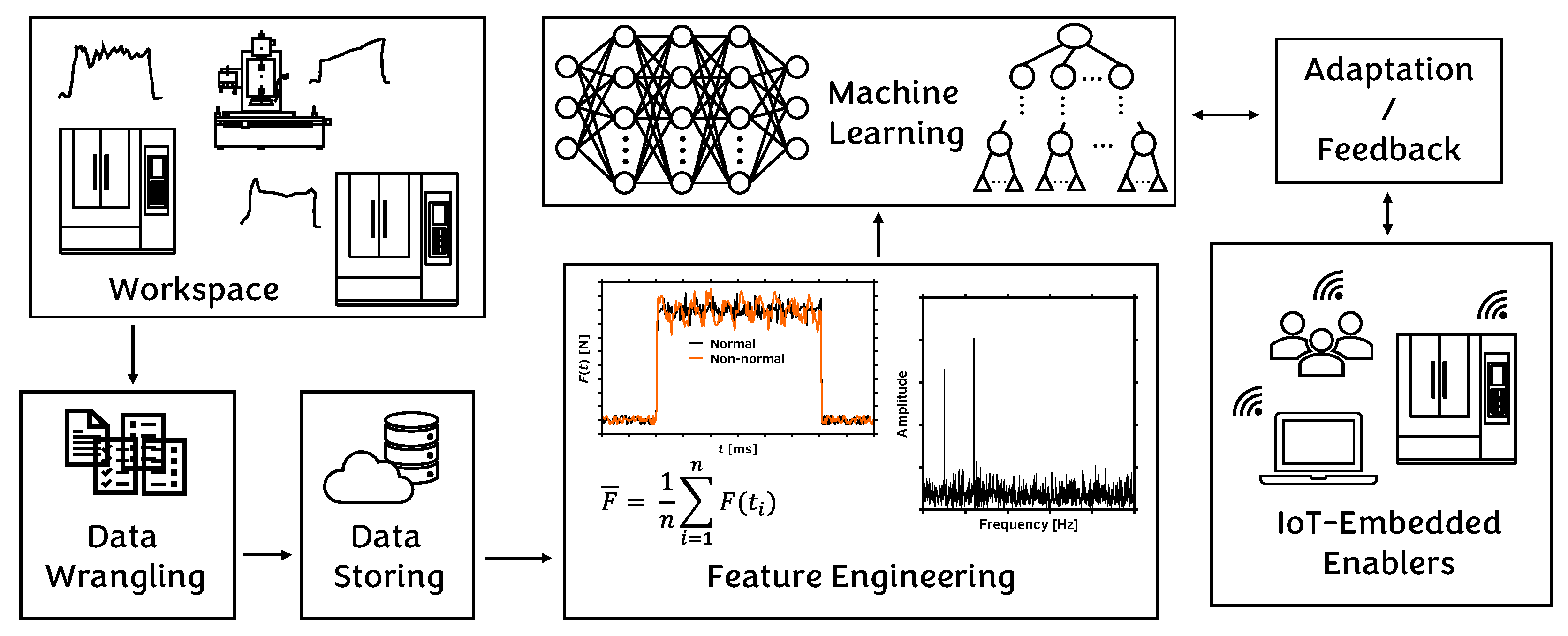
Figure 1. Outlining a smart manufacturing workflow, illustrating how data streams are processed to support cognitive tasks.
Make 07 00096 g001
Figure 2. Schematic overview of this study.
Make 07 00096 g002
Figure 3. Examples of Normal and Abnormal datasets prepared with long windows (a,c,e) and short windows (b,d,f), showing that shorter windows obscure the distinction between patterns.
Make 07 00096 g003
Figure 4. Outlining a traditional feature engineering-based ANN approach for pattern recognition.
Make 07 00096 g004
Figure 5. Integrating DBC and ANN. (a) Outlining type-2 DBC and (b) Outlining the proposed DBC-ANN approach for pattern recognition.
Make 07 00096 g005aMake 07 00096 g005b
Figure 6. Pairwise scatter plots of time-domain features (Flj | j = 1, …, 7) extracted from long-window training datasets (Xl).
Make 07 00096 g006
Figure 7. Pairwise scatter plots of time-domain features (Fsj | j = 1, …, 7) extracted from short-window training datasets (Xs).
Make 07 00096 g007
Figure 8. Feature importance score for (a) long and (b) short window.
Make 07 00096 g008
Figure 9. Performance of feature-based ANN model subjected to long window (ANN1) in (a) training and (b) testing phases.
Make 07 00096 g009
Figure 10. Performance of feature-based ANN model subjected to short window (ANN2) in (a) training and (b) testing phases.
Make 07 00096 g010
Figure 11. Results of the type-2 DBC for the training datasets with long window. (a) network of protein arrays (or, protein-verse) and their constituents and (b) examples showing Normal arrays dominated by ‘I’ and Abnormal arrays with increased ‘L, V, R, Y’.
Make 07 00096 g011
Figure 12. Results of the type-2 DBC for short window training datasets. (a) network of protein arrays (or, protein-verse) and their constituents and (b) examples showing Normal arrays with high ‘I’ and Abnormal arrays with increased ‘L, V, R, Y’.
Make 07 00096 g012
Figure 13. Hamming distances between normal and abnormal arrays for (a) long and (b) short window training datasets.
Make 07 00096 g013
Figure 14. Performance of DBC-based ANN model subjected to long window (ANN3) in (a) training and (b) testing phases.
Make 07 00096 g014
Figure 15. Performance of DBC-based ANN model subjected to short window (ANN4) in (a) training and (b) testing phases.
Make 07 00096 g015
Figure 16. The 20-fold MCCV for feature-based ANN with short window. (a) training and testing accuracy per fold and (b) accuracy difference per fold.
Make 07 00096 g016
Figure 17. Results of the 20-fold MCCV for the DBC-based ANN with a short window. (a) training and testing accuracy per fold and (b) accuracy difference per fold.
Make 07 00096 g017
Table 1. Outlining data preparation.
StepsDescriptions
Creation100 datasets are created: 50 Normal, 50 Abnormal, following the definitions in [30].
SplittingUsing stratified sampling, the datasets are divided into training and test sets, each containing 50.
WindowingLongThe training and test sets are processed with a long window size of 150, resulting in long-windowed datasets.
ShortThe training and test sets are processed with a short window size of 10, resulting in short-windowed datasets.
Note that one may access the datasets using the URL: https://github.com/commons-repo/001-research-data.git (accessed on 20 August 2025). One may also access them via the GitHub CLI (command line interface) using the command: gh repo clone commons-repo/001-research-data.
Disclaimer/Publisher’s Note: The statements, opinions and data contained in all publications are solely those of the individual author(s) and contributor(s) and not of MDPI and/or the editor(s). MDPI and/or the editor(s) disclaim responsibility for any injury to people or property resulting from any ideas, methods, instructions or products referred to in the content.