Distributionally Robust Bayesian Optimization via Sinkhorn-Based Wasserstein Barycenter

Abstract

This paper introduces a novel framework for Distributionally Robust Bayesian Optimization (DRBO) with continuous context that integrates optimal transport theory and entropic regularization. We propose the sampling from the Wasserstein Barycenter Bayesian Optimization (SWBBO) method to deal with uncertainty about the context; that is, the unknown stochastic component affecting the observations of the black-box objective function. This approach captures the geometric structure of the underlying distributional uncertainty and enables robust acquisition strategies without incurring excessive computational costs. The method incorporates adaptive robustness scheduling, Lipschitz regularization, and efficient barycenter construction to balance exploration and exploitation. Theoretical analysis establishes convergence guarantees for the robust Bayesian Optimization acquisition function. Empirical evaluations on standard global optimization problems and real-life inspired benchmarks demonstrate that SWBBO consistently achieves faster convergence, good final regret, and greater stability than other recently proposed methods for DRBO with continuous context. Indeed, SWBBO outperforms all of them in terms of both optimization performance and robustness under repeated evaluations.

1. Introduction

Modern decision-making systems are increasingly ascendant in situations of distributional uncertainty, where data-generating processes are subject to shifts, perturbations, or misspecifications at the base level. This is most salient for black-box optimization situations, where expensive function evaluations are performed under uncertain contextual settings. Although vanilla Bayesian Optimization (BO) is known to be effective for deterministic or well-characterized stochastic settings [1,2,3], it can exhibit poor out-of-sample performance when the true distribution deviates from prior assumptions. In Sample Average Approximation (SAA) methods, this phenomenon is often referred to as the “optimizer’s curse”.

Distributionally Robust Optimization (DRO) emerged as a justified methodology for addressing such uncertainties through optimization under worst-case scenarios that are aligned with carefully crafted ambiguity sets around empirical samples, e.g., historical data. Instead of point estimates of unknown distributions, DRO considers all possible distributions aligned with a neighbourhood of the empirical distribution, providing performance guarantees that degrade gracefully under shifts of the underlying distributions. Its underlying intuition is that through hedging against the uncertainty of distributions, decision-makers can gain solutions that share robust performance under a variety of plausible scenarios, even if at the cost of nominal optimality under ideal conditions.

Applying DRO concepts to BO presents a number of characteristic challenges that make it different from classical robust optimization [4]. To begin with, the black-box nature of expensive objective functions demands explicit balancing of exploration versus exploitation, simultaneously coping with distributional uncertainty. Traditional acquisition functions must be fundamentally reconsidered to incorporate robustness considerations without sacrificing the sample efficiency that makes BO attractive for expensive optimization problems. Second, the construction of appropriate ambiguity sets becomes critical in the BO setting, where limited samples must inform both the underlying surrogate model of the black-box objective function and the distributional uncertainty quantification. The choice of distance metric for defining ambiguity sets—whether based on φ-divergences, Wasserstein distances, or moment-based constraints—has a significant impact on both computational tractability and the quality of robust solutions. Recent theoretical work by Ref. [5] shows that worst-case expectation problems can be transformed into finite convex problems for many practical loss functions, which provides a foundation for tractable distributionally robust formulations. Third, the high-dimensional nature of many practical optimization problems exacerbates the curse of dimensionality in distributional uncertainty quantification. As noted by Ref. [6], distance metrics defined in high-dimensional spaces can lead to exceedingly large ambiguity sets, potentially resulting in overly conservative solutions. This observation points to the need for more sophisticated approaches that can capture the geometric structure of data distributions while maintaining computational efficiency.

Current approaches to Distributionally Robust Bayesian Optimization (DRBO) have several limitations that this work addresses. Existing methods usually rely on simple empirical averaging or uniform sampling within ambiguity sets, which fail to capture the underlying geometric structure of the context distribution. This approach can lead to suboptimal representation of distributional uncertainty and, consequently, poor exploration strategies in the robust optimization landscape [7,8].

Furthermore, many existing robust BO methods exhibit excessive conservatism, especially when ambiguity sets are large compared to the available data. The resulting solutions may sacrifice significant performance under nominal conditions to hedge against unlikely worst-case scenarios. The challenge lies in developing acquisition functions that can adaptively balance robustness and performance as more information becomes available through the optimization process. Computational complexity presents another significant barrier, as the nested min–max formulation inherent in distributionally robust optimization introduces substantial computational overhead. Traditional approaches often need to solve complex optimization problems at each iteration, making them impractical for high-dimensional or time-sensitive applications. Recent work by Ref. [9] addressed Wasserstein Distributionally Robust Bayesian Optimization (WDRBO) with continuous contexts, establishing sublinear regret bounds for settings where context distributions are uncertain but lie within Wasserstein ball ambiguity sets. However, both proposed approaches still have difficulty efficiently aggregating distributional information while preserving geometric structure.

This paper introduces a novel methodology that addresses these limitations through the principled application of the Wasserstein Barycenter, efficiently computed via the Sinkhorn regularization. Our key insight is that the geometric structure of distributional uncertainty can be effectively captured using Wasserstein Barycenter, which provides a natural generalization of the notion of mean distributions in the space of probability measures. The Wasserstein Barycenter, also known as the Fréchet mean, computed in the space of probability distributions endowed with Wasserstein distance [10], offers a non-linear interpolation mechanism that preserves the geometric characteristics of constituent distributions. Unlike simple weighted averages that ignore spatial structure, the Wasserstein Barycenter gives us a principled approach to aggregating multiple plausible distributions while maintaining their essential geometric properties. Our methodology takes advantage of the computational efficiency of the Sinkhorn algorithm to approximate Wasserstein Barycenter computation. While this approach trades the traditional distance properties for divergence measures, it provides crucial advantages: computational tractability for practical applications and guaranteed uniqueness of solutions. By combining entropic regularization with iterative scaling techniques, Sinkhorn achieves significant computational speedups while preserving the essential geometric properties required for robust optimization. The resulting Distributionally Robust Sinkhorn Barycenter Upper Confidence Bound acquisition function seamlessly integrates distributional robustness considerations into the BO framework while maintaining the exploration–exploitation balance that characterizes effective acquisition strategies. Our approach incorporates adaptive robustness scheduling and distributional Lipschitz regularization to ensure that the level of conservatism appropriately adapts to the available information and problem structure.

The main contributions of this work can be summarized as follows:

We propose SWBBO, a novel Bayesian Optimization algorithm that integrates Sinkhorn-regularized Wasserstein Barycenters into a robust acquisition strategy, providing geometry-aware modeling of distributional uncertainty in continuous contexts.

We develop a computationally efficient and theoretically grounded acquisition function that combines entropic optimal transport, adaptive robustness scheduling, and distributional Lipschitz regularization, offering strong regret guarantees under distributional shifts.

We demonstrate that SWBBO outperforms existing DRBO methods on both synthetic benchmarks and real-world-inspired optimization tasks, achieving faster convergence and improved robustness under repeated evaluations.

The rest of this paper proceeds in the following manner. We begin with Section 2, which covers essential background on DRO and Wasserstein Barycenter. In Section 3, we describe the DRBO framework, along with the Sinkhorn-regularized barycenter computation and the acquisition function. Section 4 formalizes the problem setting, introduces our distributional robustness framework, and presents the core methodology. Section 5 presents a comprehensive experimental evaluation, and Section 6 concludes with a discussion of future research directions.

2. Literature Review

2.1. Theoretical Foundations of DRO

The theoretical foundations of Distributionally Robust Optimization (DRO) have advanced significantly in recent years, revealing important connections between robust statistical methods and optimization under distributional uncertainty. In 2022, Rahimian and Mehtora published a comprehensive survey [11] that thoroughly covers the field, tracing its evolution from classical robust optimization to modern distributionally robust approaches. Their work categorizes different types of ambiguity sets—including moment-based, distance-based, and divergence-based formulations—and examines the trade-offs between robustness guarantees and computational feasibility. Building on this foundation, Ref. [5] demonstrates that many DRO problems can be seen as extensions of robust statistical estimation methods. Rather than simply looking for robust parameter estimates, the focus shifts toward finding decisions that work well across multiple plausible data-generating distributions. The authors in Ref. [12] took these concepts further by developing adaptive DRO frameworks that dynamically adjust ambiguity sets as new data become available. This method addresses the fundamental challenge of balancing robustness with performance in sequential decision-making, providing a way to reduce the excessive conservatism typical of worst-case optimization while maintaining strong out-of-sample guarantees. This work tackles key problems found in traditional stochastic optimization (SO) methods that depend on fixed probability distributions. DRO’s mathematical framework handles uncertainty using three main paradigms. SO represents the first approach, which maximizes expected performance under a known distribution [7]:

$$\underset{x\in \mathcal{X}\subset {\mathbb{R}}^d}{\mathit{max}}{E}_{c\sim P}\left[f\right(x,c\left)\right]$$

(1)

Let $x\in \mathcal{X}\subset {\mathbb{R}}^d$ denote the decision variables, and $c\sim P$ denote the context. The function $f\left(x,c\right)$ is the black-box objective function to be minimized, which depends on both decision and contextual variables. Decisions are made assuming perfect knowledge of the probability distribution P governing uncertain parameters c. Worst-case Robust Optimization (RO) adopts an extremely conservative approach by optimizing against the worst possible realization:

$$\underset{x\in \mathcal{X}\subset {\mathbb{R}}^d}{\mathit{max}} \underset{c\in \Delta }{\mathit{min}} f\left(x,c\right),$$

(2)

where no probabilistic assumptions are made about the uncertainty set Δ.

Finally, DRO achieves a balanced compromise through optimizing against the worst-case expectation over all distributions Q within an ambiguity set U.

$$\underset{x\in \mathcal{X}\subset {\mathbb{R}}^d}{\mathit{max}} \underset{Q\in \mathcal{U}}{ \mathit{Inf}} E_{c\sim Q} \left[f\right(x,c\left)\right],$$

(3)

In the following formulations, $f(x,c)$ represents the objective function evaluated at decision $x$ under context $c$. Depending on the optimization paradigm, we take expectations over $c$, worst-case realizations, or robust expectations over an ambiguity set.

2.2. Wasserstein Distance and Optimal Transport

In statistics and machine learning, the Wasserstein distance has increasingly gained importance as it allows the comparison of probability distributions of different types while satisfying all properties of a distance metric under certain assumptions. It has been recently applied to extend BO on complicated—also known as exotic—tasks such as grey-box optimization [13] and multiple information source optimization [14].

The mathematical foundation for the p-Wasserstein distance between probability measures α and β in P(Ω) is defined as [15]

$$W_p^p(\alpha ,\beta )=\underset{\pi \in \Pi (\alpha ,\beta )}{\mathit{Inf}}\underset{\Omega \times \Omega }{\int }{d}^p(\omega ,{\omega }^{\prime })d\pi (\omega ,{\omega }^{\prime })$$

(4)

where $\Pi (\alpha ,\beta )$ is the set of probability measures on $\Omega \times \Omega$ having marginals α and $\beta$, and $p \ge 1$. $\omega$ and ${\omega }^{\prime }$ are probability measures (i.e., distributions) over the space $\Omega$, and $\pi (\omega ,{\omega }^{\prime })$ denotes the set of joint couplings (transport plans) with marginals $\omega$ and ${\omega }^{\prime }$. Setting $p = 2$ and $d(.,.)$ the Euclidean distance leads to the so-called 2-Wasserstein distance with Equation (4) that can be rewritten as

$$W_2^2(\alpha , \beta )=\underset{T_{\#}\alpha =\beta }{\mathit{min}}\underset{\Omega }{\int }{\parallel T\left(\omega \right)-\omega \parallel }_2^{2}d\alpha (\omega )$$

(5)

which is intended as an optimal transport problem [10]. This formulation interprets the distance as the minimum cost of transporting probability mass $\alpha$ to match target probability mass $\beta$, where symbol # denotes the push-forward operator ensuring that α matches $\beta$ following transport plan T.

For Gaussian distributions, that is $\alpha =\mathcal{N}(m_{\alpha }, {\Sigma }_{\alpha })$ and $\beta =\mathcal{N}(m_{\beta }, {\Sigma }_{\beta })$, the 2-Wasserstein distance simplifies to [9]

$$W_2^2 (\alpha , \beta )={\parallel m_{\alpha }-m_{\beta }\parallel }^2\mathcal{ }\mathcal{ }+\mathcal{ }\mathcal{B}{({\Sigma }_{\alpha }, {\Sigma }_{\beta })}^2$$

(6)

where $\mathcal{B}$ represents the Bures metric between positive definite matrices [16,17]:

$$\mathcal{B}{({\Sigma }_{\alpha }, {\Sigma }_{\beta })}^2 = trace\left({\Sigma }_{\alpha } +{\Sigma }_{\beta } - 2{\left({\Sigma }_{\alpha }^{{\displaystyle \frac{1}{2}}} {\Sigma }_{\beta } {\Sigma }_{\alpha }^{{\displaystyle \frac{1}{2}}} \right)}^{{\displaystyle \frac{1}{2}}}\right)$$

(7)

Thus, in the case of centered GDs (i.e., $m_{\alpha }= m_{\beta }=0)$, the 2-Wasserstein distance resembles the Bures metric. Moreover, if ${\Sigma }_{\alpha }$ and ${\Sigma }_{\beta }$ are diagonal, the Bures metric is the Hellinger distance, while in the commutative case, that is ${\Sigma }_{\alpha }{\Sigma }_{\beta }$ = ${\Sigma }_{\beta }{\Sigma }_{\alpha }$, the Bures metric is equal to the Frobenius norm $\parallel {\Sigma }_{\alpha }^{{\displaystyle \frac{1}{2}}} - {\Sigma }_{\beta }^{{\displaystyle \frac{1}{2}}} {\parallel }_{Frobenius}^2$.

When dealing with general probability distributions beyond the Gaussian case, computing the Wasserstein distance becomes much more difficult and requires solving the Monge or Kantorovich optimal transport problems. The Kantorovich formulation turns this into a linear program with $O(n^3 log n)$ complexity for discrete measures on n points, which makes exact computation impractical for large-scale applications. This computational burden has motivated the development of entropic regularization techniques that approximate the optimal transport solution while maintaining computational tractability.

The computational tractability of Wasserstein-based methods has been revolutionized through entropic regularization approaches, most notably the introduction of Sinkhorn distances [18], which enables rapid computation of optimal transport through entropic penalties. Recent complexity analyses have improved our understanding of entropic regularized algorithms for optimal transport between discrete probability measures, establishing refined convergence bounds and computational guarantees [19]. The extension to Wasserstein Barycenter computation through fast Sinkhorn-based algorithms [15] has established the algorithmic foundations for practical implementation while maintaining essential geometric properties with significant computational speedups.

2.3. Wasserstein Barycenters and Geometric Averaging

The mathematical foundations for geometric averaging of probability distributions are rooted in optimal transport theory and the concept of Wasserstein Barycenters.

Given a set of probability measures ${\left\{{\alpha }_i\right\}}_{i=1}^N$ in $\mathbb{P}\subset P(\Omega )$ with associated weights ${\left\{{\lambda }_i\right\}}_{i=1 }^N$ with ${\sum }_{i=1}^N{\lambda }_i = 1$, their Wasserstein Barycenter $\overline{\alpha }$ is defined as

$$\overline{\alpha }\in \underset{\alpha \in \mathbb{P}\subset \mathit{P }(\Omega )}{\mathit{argmin}}{\sum }_{i=1}^N{\lambda }_i{W}_2^2\left(\alpha , {\alpha }_i\right)$$

(8)

where $\overline{\alpha }$ is uniquely defined by the weights ${\left\{{\lambda }_i\right\}}_{i=1 }^N$. Thus, different weights lead to a different Wasserstein Barycenter. The most common situation is to consider equally weighted probability measures, that is ${\lambda }_i=1/N,\forall i=1,\dots ,N$, leading to

$$\overline{\alpha }\in \mathrm{ }\mathrm{ }\underset{\alpha \in \mathbb{P}\subset P\mathrm{ }\left(\mathrm{\Omega }\right)}{\mathit{arg}\min }1/N{\sum }_{\mathrm{i}=1}^N{W}_2^2\left(\alpha ,\mathrm{ }{\alpha }_i\right)$$

(9)

For univariate Gaussian distributions ${\alpha }_i=\mathcal{N}(m_i,{\sigma }_i)$, the Wasserstein Barycenter $\overline{\alpha }=\mathcal{N}(\overline{m},\overline{\sigma })$ has parameters determined by

$$\overline{m}, \overline{\sigma } \in \underset{m,\sigma }{\mathit{argmin}}{\displaystyle \frac{1}{N}}{\sum }_{i=1}^N\left[{\left(m_i-m\right)}^2 +{\left({\sigma }_i-\sigma \right)}^2 \right]$$

(10)

The solution is elegantly simple: $\overline{m}=1/N{\sum }_{\mathrm{i}=1}^N{m}_i$ and $\overline{\sigma }=1/N{\sum }_{\mathrm{i}=1}^N{\sigma }_i$. This demonstrates that Wasserstein Barycenters of Gaussian distributions preserve the Gaussian structure while averaging parameters in the natural geometric space.

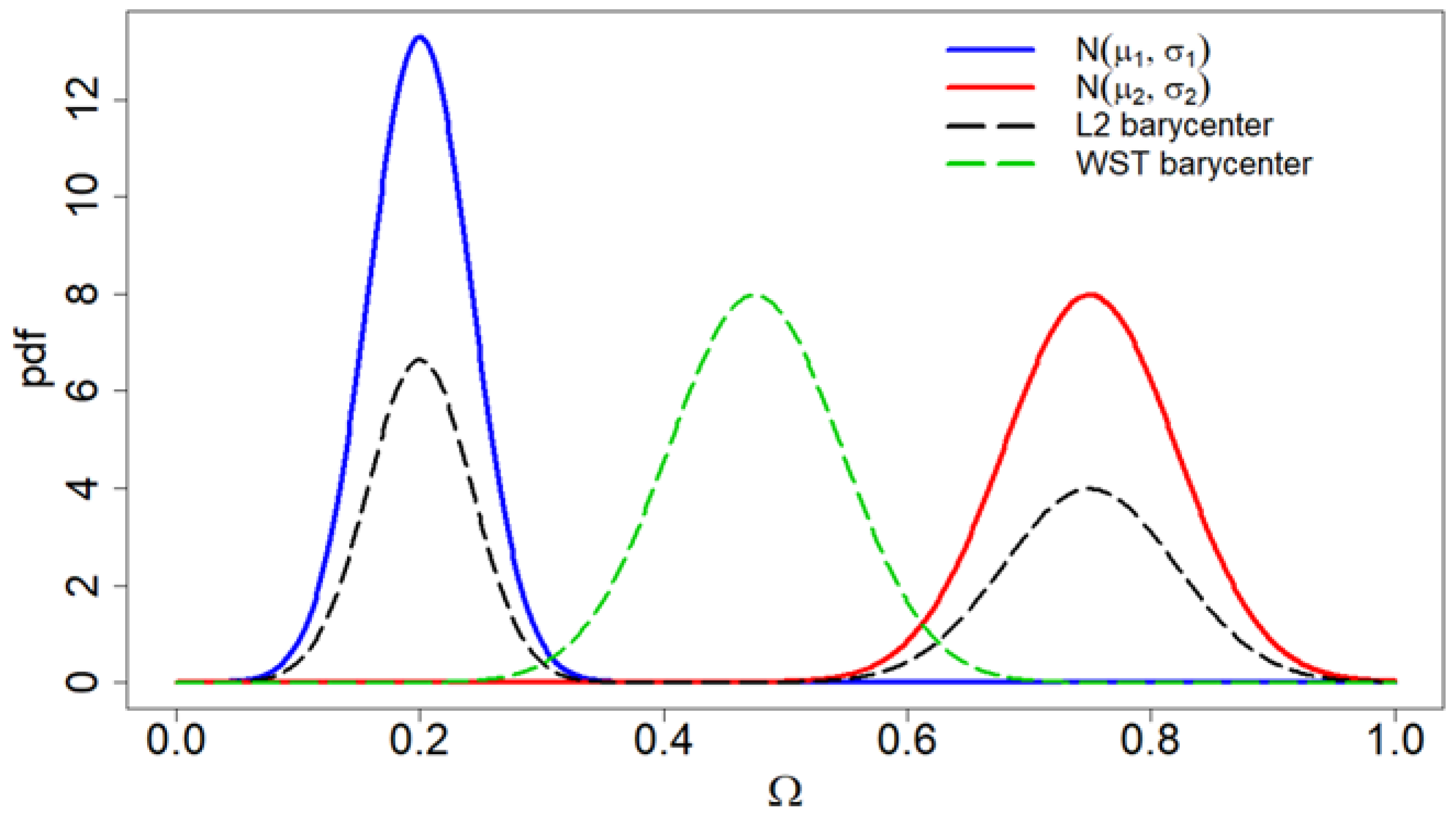
Figure 1 provides a practical and simple example showing the difference between the Wasserstein Barycenter of two (equally weighted) normal distributions and the L2-norm barycenter obtained by considering, as the distance, the L2-norm between the probability density functions aligned on the support. The shape preservation guaranteed by the Wasserstein Barycenter is clearly visible: it is normal, instead of bimodal.

Wasserstein Barycenters generalize McCann’s interpolation to the case of more than two measures, providing a natural extension of mean distributions that preserves geometric structure in probability spaces [20]. Recent theoretical advances have established both the fundamental importance and computational complexity of these objects, with Wasserstein Barycenters being proven NP-hard to compute in general settings [21], highlighting the necessity for efficient algorithmic approximations.

2.4. Ambiguity Set Construction and Distance Metrics

Constructing ambiguity sets is one of the most important design decisions in DRO, since different distance metrics create entirely different optimization problems and computational challenges. Ref. [22] came up with a new data-driven approach that relies on statistical hypothesis tests to build uncertainty sets that balance robustness with performance. This gives us principled statistical frameworks instead of arbitrary specifications. They use historical data to figure out appropriate robustness levels and incorporate complex statistical testing procedures that can handle intricate dependency structures.

There are several basic ways to construct ambiguity sets in DRO. Moment-based ambiguity sets work by constraining the mean, variance, and higher-order moments. While these are computationally manageable, they often miss important aspects of the distribution. Divergence-based ambiguity sets create neighborhoods around reference measures using metrics like Kullback–Leibler divergence [17] or Total Variation distance. These have solid theoretical backing but can be hard to interpret geometrically. Wasserstein-based ambiguity sets offer flexible and intuitive frameworks that use optimal transport metrics to measure distributional distances, which gives us both computational feasibility and meaningful geometric understanding.

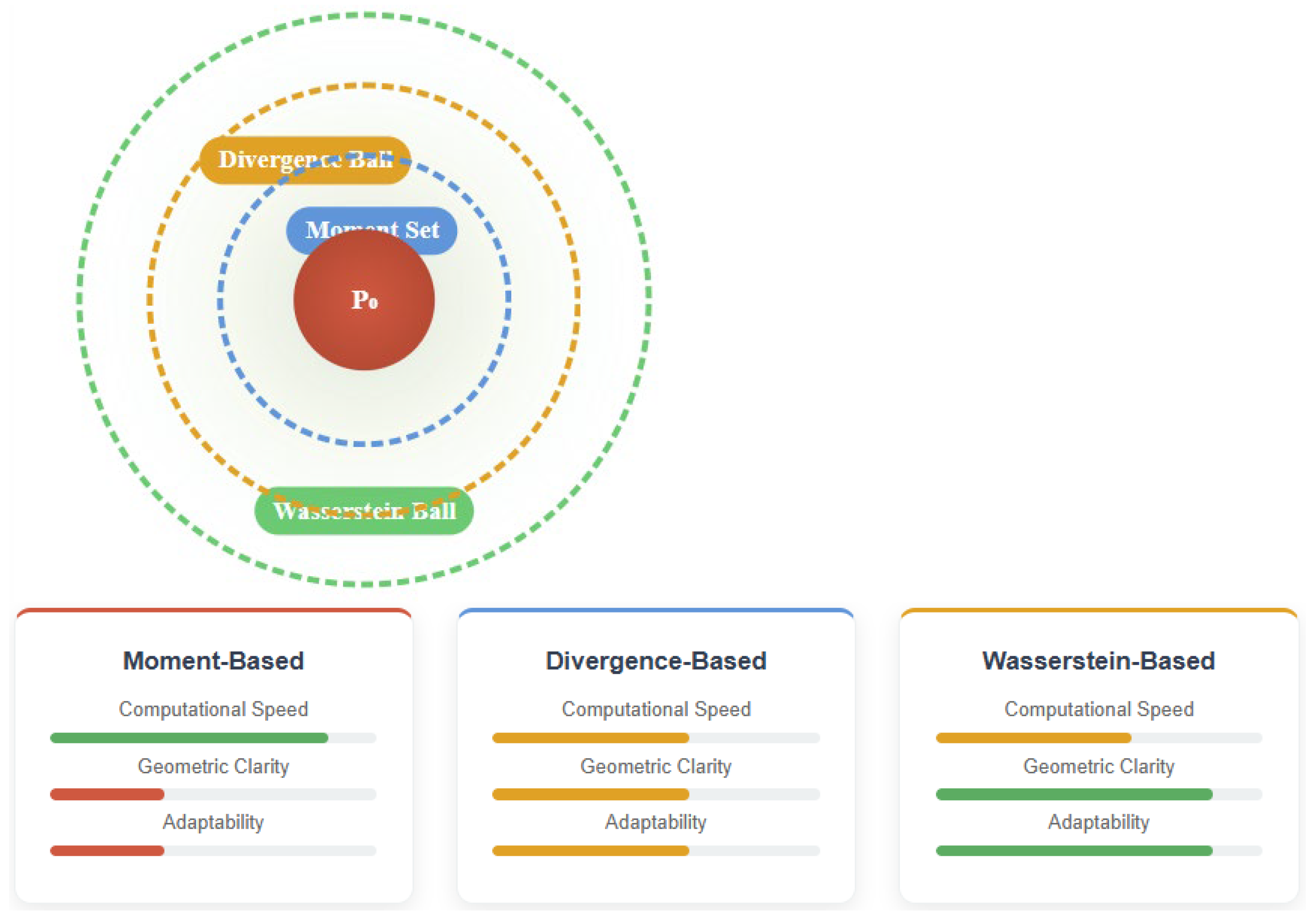
Wasserstein-based methods have become popular among these options because they can handle realistic transportation costs and come with strong theoretical guarantees. Figure 2 shows the three main ways to construct ambiguity sets in DRO, illustrating how moment-based, divergence-based, and Wasserstein-based methods create different-sized uncertainty neighborhoods around the reference distribution. The figure highlights the trade-offs between computational ease, geometric understanding, and methodological flexibility across these different approaches.

Computational Speed. How fast and practical it is to solve the resulting optimization problem.

Geometric Clarity. How easy it is to understand the geometric meaning of distributional distances and uncertainty neighborhoods (Wasserstein methods give clear transportation cost intuition, while moment-based methods involve abstract statistical constraints).

Adaptability. How well the method can handle different problem types, cost functions, and distributional characteristics (Wasserstein methods can adjust cost functions for specific uses, while moment-based methods are stuck with fixed moment structures).

Building on these foundations, Ref. [24] made significant theoretical contributions to optimal transport-based DRO, establishing crucial structural properties of the value function in Wasserstein-based DRO problems and developing efficient iterative solution schemes. The computational implications of different ambiguity set constructions vary significantly depending on the chosen distance metric, with Wasserstein-based methods requiring more sophisticated optimal transport algorithms but providing valuable geometric insights, particularly in high-dimensional settings where traditional distance metrics may be overly conservative.

2.5. BO Challenges

Traditional BO approaches run into several basic problems that have pushed researchers to develop distributionally robust extensions. DRBO methods specifically handle uncertainty in the underlying probability distribution of the objective function, which is affected by unknown stochastic noise. Ref. [9] shows how Wasserstein-based distributionally robust approaches can give theoretical guarantees even when the model is misspecified. Meanwhile, Ref. [4] lays out the mathematical foundations for incorporating distributional ambiguity. More generally, Wasserstein Distributionally Robust Optimization (WDRO) has become a solid framework for dealing with distributional uncertainty across different optimization problems [25,26]. It provides robustness guarantees that stay valid when the true distribution falls within a specified Wasserstein ball around the empirical distribution. This way of thinking about distributional robustness changes the focus from obtaining perfect model specification to developing optimization strategies that work well across a range of plausible distributions. This makes the approach more practical for real-world applications where we are inherently uncertain about distributional assumptions.

2.6. Acquisition Functions for DRBO

Standard acquisition functions must be adapted for the distributionally robust setting. The key challenge is incorporating distributional uncertainty into the acquisition strategy while maintaining computational tractability.

For UCB-based approaches, the robust acquisition function typically takes the following form:

$${\alpha }_{R-UCB}(x)={\underset{P\in \mathcal{U}}{\min }\mathbb{E}}_{\mathrm{P}}[{\mu }_n(x,c)+{\beta }_n{\sigma }_n(x,c)]$$

(11)

where $\mathcal{U}$ is the ambiguity set over distributions of the context, which is unknown a priori, ${\mu }_n$ and ${\sigma }_n$ are the GP’s posterior mean and standard deviation, after $n$ observations, and ${\beta }_n$ is a parameter controlling the exploration–exploitation trade-off.

However, simple empirical averaging over observed contexts may not capture the underlying structure of the context distribution, motivating the adoption of the Wasserstein ball ambiguity set and, due to the need for computational efficiency, the Sinkhorn regularization.

2.7. Integrating Distributionally Robust Principles into BO

Combining BO with DRO has become a new framework for tackling both parametric uncertainty and distributional uncertainty in data-driven optimization problems. Ref. [27] introduced Bayesian Distributionally Robust Optimization (BDRO), which builds a comprehensive theoretical foundation that differs from traditional DRO approaches by including Bayesian estimation of unknown parametric distributions. Their framework builds ambiguity sets using parametric distributions as reference points, which allows for robust optimization that keeps the benefits of Bayesian estimation when data are scarce while providing robustness against model uncertainty.

Extending distributionally robust principles to BO is a recent development that tackles expensive function evaluation under distributional uncertainty. Ref. [28] worked on black-box optimization problems that include both design variables and uncertain context variables. They handled both aleatoric and epistemic uncertainty sources using adaptive and safe optimization strategies in high-dimensional spaces. Ref. [9] made important progress by tackling situations where context distributions are uncertain, but we know they fall within ambiguity sets defined as balls in the Wasserstein space. The researchers established sublinear regret bounds that give us theoretical guarantees for how DRBO algorithms converge. These developments together show that DRBO has matured into a unified framework that can handle both parametric and distributional uncertainties in complex decision-making situations.

DRBO brings several unique challenges compared to standard BO:

Ambiguity Set Construction: The choice of ambiguity set $\mathcal{U}$ significantly impacts the robustness performance trade-off. People typically use Wasserstein balls, ϕ-divergence balls, and moment-based sets [23].

Computational Complexity: The min–max formulation creates a nested optimization problem that is still computationally difficult even with recent algorithmic improvements. Modern approaches use dual formulations and cutting-plane methods to deal with the computational burden of continuous ambiguity sets [11,29,30,31], but scaling up to high-dimensional problems is still an active area of research.

Conservative Solutions: DRBO can produce overly conservative solutions when the ambiguity set is not sized correctly. Recent work has focused on developing principled approaches for ambiguity set calibration that balance being conservative with maintaining good performance. This includes adaptive shrinking strategies and risk-aware formulations [32,33]. One key limitation is sample efficiency: when you are dealing with distributional uncertainty, it takes longer for the algorithm to converge compared to standard Bayesian Optimization. This happens because the algorithm needs to protect itself against multiple possible scenarios that could play out. To address this problem, current research is working on better acquisition function designs and multi-fidelity approaches that can reduce the computational burden that comes with distributional robustness [34].

2.8. Computational Challenges and High-Dimensional Considerations

The curse of dimensionality creates fundamental challenges in DRO, since traditional distance metrics can produce prohibitively large ambiguity sets and overly conservative performance guarantees in high-dimensional spaces. Ref. [35] tackled this critical limitation by developing the first finite-sample guarantees for Wasserstein DRO that break the curse of dimensionality. Their groundbreaking work demonstrates how the out-of-sample performance of robust solutions depends on sample size, uncertainty dimension, and loss function complexity in a nearly optimal manner, providing theoretical foundations that make high-dimensional Wasserstein DRO practically viable. Their groundbreaking work shows how the out-of-sample performance of robust solutions depends on sample size, uncertainty dimension, and loss function complexity in a nearly optimal manner, providing theoretical foundations that make high-dimensional Wasserstein DRO practically viable. The theoretical foundations established by Ref. [23] provided essential performance guarantees and tractable reformulations for data-driven DRO using the Wasserstein metric, enabling practical implementations that have significantly influenced subsequent algorithmic developments. Ref. [25] showed that data-driven Wasserstein DRO can achieve workable reformulations and strong performance guarantees when you properly account for the underlying geometry of the problem. They found that Wasserstein ambiguity sets naturally regularize the system, which helps prevent overfitting when you are working with limited samples.

Recent developments include advanced generic column generation algorithms for high-dimensional multimarginal optimal transport problems, which allow for accurate mesh-free Wasserstein Barycenters and cubic Wasserstein splines [36]. The comprehensive theoretical framework from Ref. [10] continues to support modern computational optimal transport applications with solid convergence properties and approximation bounds for practical data science uses.

2.9. Research Gaps

This literature review shows critical computational and theoretical gaps in DRBO that standard approaches simply cannot address. Current robust BO methods face two key problems: first, naive aggregation strategies like uniform weighting across uncertainty sets completely ignore how probability spaces are actually structured, which leads to suboptimal acquisition functions that work less efficiently than methods that understand distributions better. Second, existing Wasserstein-based approaches need to solve transport problems at every single BO iteration, which creates major bottlenecks and makes them too slow to use in practice. The real problem here is keeping distributional geometry intact during optimization. When uncertainty sets contain distributions that have completely different support or covariance structures, simply averaging them destroys the geometric relationships that actually drive good exploration–exploitation trade-offs. Our Sinkhorn-regularized approach tackles this computational barrier head-on by approximating Wasserstein Barycenters while keeping geometric fidelity within ε-accuracy of exact solutions. But we still face three unresolved challenges: handling distributional uncertainty sets that span different support dimensions, keeping barycenter approximation quality stable as the ambient space dimension grows, and developing adaptive regularization parameters that can balance computational speed against geometric precision across different types of problems. This points to a clear need for developing computationally practical methods that preserve essential distributional geometry without giving up the convergence guarantees that make BO useful for expensive optimization problems.

3. Sinkhorn Barycenter Upper Confidence Bound for DRBO

This section walks through our Sinkhorn Barycenter Upper Confidence Bound (SB-UCB) approach for DRBO. We start by setting up the DRBO framework and laying out the minimax optimization problem when we are dealing with distributional uncertainty (Section 3.1). Then we show how to extend standard GP modeling so it can handle both contextual variables and decision variables together (Section 3.2). The key innovation here is how we build Wasserstein-based ambiguity sets (Section 3.3) and use Sinkhorn-regularized Wasserstein Barycenters to create robust distributional representations (Section 3.4). Here is how it works: we take the empirical context distribution and split it into multiple candidate distributions, then compute their entropic-regularized Wasserstein Barycenter to obtain a single representative distribution. This representative distribution keeps the important geometric structure while still accounting for distributional uncertainty. We then use this barycenter distribution in our robust acquisition function to make optimization both safe and efficient.

3.1. DRBO Framework

DRBO tackles optimization problems where we are not sure about the underlying data-generating distribution, which means it extends traditional BO to handle situations where we have distributional ambiguity ([11,28]). This approach is especially useful in real-world applications like robust hyperparameter tuning when datasets shift over time, autonomous systems that need to work under uncertain environmental conditions, and Portfolio Optimization, where we face model risk ([37,38]).

The DRO problem is formulated as

$$\mathrm{x}\mathrm{*}=\underset{\mathrm{x}\in \mathcal{X}\subset {\mathbb{R}}^{\mathrm{d}}}{\mathrm{argmax}}\underset{P\in \mathcal{U}}{ \min }{\mathbb{E}}_{c\sim P}\left[f(x,c)\right]$$

(12)

where $x\in \mathcal{X}\subseteq {\mathbb{R}}^d$ represents the decision variables, $c\in \mathcal{C}\subseteq {\mathbb{R}}^k$ denotes the context variables, and $f:\mathcal{X}\times \mathcal{C}\to \mathbb{R}$ is an unknown objective function. $\mathcal{U}$ is the ambiguity set containing plausible distributions.

In practice, we construct the ambiguity set from empirical observations, leading to

$$\mathrm{x}\mathrm{*}=\underset{\mathrm{x}\in \mathcal{X}}{\mathrm{argmax}}{\underset{P\in {\mathcal{U}}_n}{ \min }\mathbb{E}}_{c\sim P}\left[f(x,c)\right]$$

(13)

where ${\mathcal{U}}_n$ represents the ambiguity set constructed accordingly to n observations of the context, that is $C_n=\{c_1,c_2,\dots ,c_n\}$.

3.2. GP Modeling for DRBO

BO represents a sample-efficient model-based sequential method for global optimization of black-box, multi-extremal, and expensive-to-evaluate objective functions [1,2,3]. The fundamental problem addresses global minimization:

$$\mathrm{x}\mathrm{*}\in \mathrm{ }\mathrm{ }\arg \underset{x\in X\subset {\mathbb{R}}^h}{\min }f(\mathrm{x},\mathcal{c})$$

(14)

where $\mathcal{X}$ typically represents the h-dimensional unit hypercube $\mathcal{X}={[0,1]}^{\mathrm{h}}$, $\mathcal{c}\in \mathcal{C}\subset {\mathbb{R}}^p$ denotes the contextual variables, and $f:\mathcal{X}\times \mathcal{C}\to \mathbb{R}$ represents the expensive objective function exhibiting black-box and multi-extremal properties. The context $\mathcal{c}$ captures environmental conditions, problem parameters, or external factors that influence the objective function but are not directly controllable during optimization.

The generic iteration of BO consists of generating an approximation of $f(\mathrm{x},\mathrm{c})$ depending on previous observations ${\mathcal{D}}^{\left(n\right)}=(X,C,\mathrm{y})$, with $X={\left\{{\mathrm{x}}^{\left(i\right)}\right\}}_{i=1:n}$, $C={\left\{{\mathrm{c}}^{\left(i\right)}\right\}}_{i=1:n}$ and $\mathrm{y}={\left\{y^{\left(i\right)}\right\}}_{i=1:n}$. After that, the next query ${\mathrm{x}}^{(n+1)}$ that balances exploration and exploitation is selected, given the current context ${\mathrm{c}}^{(n+1)}$.

GP regression over the joint input space $\mathcal{X}\times \mathcal{C}$ provides the most common approximation framework, leading to GP-based BO. While $\mathcal{X}$ is the space of all the possible decision, $\mathcal{C}$ is the space of the observable—but not decidable—contexts. The GP predictive equations for mean and variance are

$$\mathrm{\mu }\left(\mathrm{x},\mathrm{c}\right)={\mathrm{\mu }}_0\left(\mathrm{x},\mathrm{c}\right)+\mathrm{k}(\left(\mathrm{x},\mathrm{c}\right),\left(\mathrm{X},\mathrm{C}\right)){[\mathrm{K}+{\mathsf{\sigma }}_{\mathsf{\epsilon }}^2\mathrm{I}]}^{-1}(\mathrm{y}-{\mathrm{\mu }}_0(\mathrm{X},\mathrm{C}))$$

(15)

$${\mathsf{\sigma }}^2(\mathrm{x},\mathrm{c})=\mathrm{k}((\mathrm{x},\mathrm{c}),(\mathrm{x},\mathrm{c}))-\mathrm{k}(\left(\mathrm{x},\mathrm{c}\right),\left(\mathrm{X},\mathrm{C}\right)){[\mathrm{K}+{\mathsf{\sigma }}_{\mathsf{\epsilon }}^2\mathrm{I}]}^{-1}\mathrm{k}(\left(\mathrm{X},\mathrm{C}\right),\left(\mathrm{x},\mathrm{c}\right))$$

(16)

where ${\mathrm{\mu }}_0\left(\mathrm{x},\mathrm{c}\right)$ represents the prior mean over the joint space, $k(·,·)$ denotes the kernel function for every pair $\left(x,c\right)$, and $K$ is the $n\times n$ kernel matrix whose entries are ${\mathrm{K}}_{\mathrm{i}\mathrm{j}}=\mathrm{k}\left(\left({\mathrm{x}}^{\left(i\right)},{\mathrm{c}}^{\left(i\right)}\right),\left({\mathrm{x}}^{\left(j\right)},{\mathrm{c}}^{\left(j\right)}\right)\right)$. Then, the acquisition function, such as GP-UCB, determines the next query given the observed context by solving

$${\mathrm{x}}^{(n+1)}\in \mathrm{ }\mathrm{ }\arg \underset{\mathrm{x}\in \mathcal{X}}{\min }{\mu }_n\left(\mathrm{x},{\mathrm{c}}^{\left(n+1\right)}\right)-{\beta }_n{\sigma }_n(\mathrm{x},{\mathrm{c}}^{(n+1)})\mathrm{ }$$

(17)

where the optimization is performed over the decision variables $x$ while conditioning on the given context ${\mathrm{c}}^{(n+1)}$.

In our implementation, we use a Matérn 5/2 kernel operating on the joint input space of decision variables and contexts. Specifically, we use an anisotropic Matérn 5/2 kernel, with a different length-scale for each dimension, as determined by Automatic Relevance Determination (ARD) [39].

3.3. Ambiguity Set Construction via Wasserstein Distance

Given empirical observations $\{c_1,c_2,\dots ,c_n\}$, we construct Wasserstein-based ambiguity sets:

$${\mathcal{U}}_{\mathrm{n}}^{\mathsf{\epsilon }}=\{\mathrm{P}:{\mathrm{W}}_2^2(\mathrm{P},{\widehat{\mathrm{P}}}_{\mathrm{n}})\le \mathrm{\epsilon }\}$$

(18)

where ${\widehat{\mathrm{P}}}_{\mathrm{n}}={\displaystyle \frac{1}{\mathrm{n}}}\sum _{\mathrm{i}=1}^{\mathrm{n}}{\mathrm{\delta }}_{{\mathrm{c}}_{\mathrm{i}}}$ is the empirical distribution and $W_2$ is the 2-Wasserstein distance.

3.4. Sinkhorn Barycenter Construction for Robust Representation

3.4.1. Distributional Uncertainty Partitioning

We partition the uncertainty space by considering multiple plausible distributions within the ambiguity set. We construct $m$ candidate distributions by

• Random Partitioning: Generate $m$ random partitions from the empirical distribution using permutation-based splitting
• Bootstrap Sampling: Generate $m$ bootstrap samples from the empirical distribution
• Balanced Partitioning: Create distributions by balanced division to ensure minimum samples per distribution

Each candidate distribution $P_i$ defines a discrete measure: ${\widehat{P}}_i={\displaystyle \frac{1}{n_i}}\sum _{j=1}^{n_i}{\delta }_{c_i^{\left(j\right)}}$. where $c_i^{\left(j\right)}$ denotes the j-th sample in candidate distribution $P_i$ derived from $\{c_1,c_2,\dots ,c_n\}$.

Figure 3 shows the three ways we can partition distributional uncertainty. Random partitioning (b) creates balanced distributions by splitting them based on permutations, bootstrap sampling (c) builds distributions by sampling with replacement, and balanced partitioning (d) takes the empirical distribution (a) and divides it step-by-step into equal-sized chunks. We chose to go with the random partitioning approach because it strikes a good balance between randomness and size constraints—this way, each distribution has enough samples to be meaningful while still creating variety across the ambiguity set {P₁, P₂, P₃}.

3.4.2. Entropic Regularized Wasserstein Barycenter for Robust Aggregation

The concept of Wasserstein Barycenters, introduced by Ref. [20], allows us to construct a representative distribution that captures the geometry of the ambiguity set. We compute the Wasserstein Barycenter of candidate distributions. Given candidate distributions $\{P_1,\dots ,P_m\}$ over $\mathcal{C}$ constructed from empirical context observations (where each $P_i$ represents a plausible distributional model of the context-generating process), the Wasserstein Barycenter $\nu \mathrm{*}$ with weights $\lambda =({\lambda }_1,\dots ,{\lambda }_m)$, where $\sum _{i=1}^m{\lambda }_i=1$, solves

$$\nu \mathrm{*}=\arg \underset{\nu \in \mathcal{P}\left(\mathcal{C}\right)}{\min }\sum _{i=1}^m{\lambda }_i{W}_2^2(\nu ,P_i)$$

(19)

where $W_2(\cdot ,\cdot )$ is the 2-Wasserstein distance, and $\mathcal{P}\left(\mathcal{C}\right)$ denotes the space of probability measures supported on the context space $\mathcal{C}$, and $P_i\in \mathcal{P}\left(\mathcal{C}\right)$. The barycenter $\nu \mathrm{*}$ provides a geometrically principled aggregation of the candidate distributions that preserves their essential structural properties while accounting for distributional uncertainty in the context generation process.

Computing exact Wasserstein Barycenters is computationally prohibitive for large datasets. Following Ref. [18] and the comprehensive treatment by Ref. [10], we employ entropic regularization to make the problem tractable. The entropic regularized optimal transport problem is

$$W_{2,\gamma }^2(\nu ,P_i)=\underset{T\in \Pi (\nu ,P_i)}{\min }⟨C,T⟩+\gamma H\left(T\right)$$

(20)

where

• $C$ is the cost matrix with $C_{ij}={‖c_i-c_j‖}_2^2$
• $\mathit{T}$ is the transport plan constrained to $\Pi (\mu ,\nu )$ (the set of couplings with marginals $\mu$ and $\nu$)
• $\gamma >0$ is the regularization parameter
• $H\left(T\right)=-{\sum }_{j,k}{T}_{jk}log{T}_{jk}$ is the entropy of the transport plan

The regularized barycenter problem becomes

$${\nu }_{\gamma }^{\mathrm{*}}=\mathit{arg}\underset{\nu \in \mathcal{P}(\mathcal{C})}{\min }\sum _{i=1}^m{\lambda }_i{W}_{2,\gamma }^2(\nu ,P_i)$$

(21)

This formulation allows for efficient computation using the Sinkhorn algorithm while preserving the essential geometric properties of the Wasserstein Barycenter [40].

4. Distributionally Robust Sinkhorn Barycenter UCB Method

This section walks through the complete algorithmic implementation of our Distributionally Robust Sinkhorn Barycenter UCB (DR-SB-UCB) method. We start by explaining the Sinkhorn algorithm and how it efficiently computes Barycenters using entropic regularization (Section 4.1). Then, we develop a robust acquisition function that maximizes UCB values over barycenter support points while adding distributional Lipschitz regularization to control how sensitive the method is to context variations, following the approach by Ref. [9] (Section 4.2). The complete SWBBO algorithm brings these components together with adaptive robustness scheduling that becomes less conservative over time (Section 4.3). Finally, we establish theoretical convergence guarantees for each part of the algorithm, including how fast Sinkhorn converges, bounds on barycenter approximation quality, and regret bounds for the overall robust optimization process.

4.1. Sinkhorn Algorithm for Robust Barycenter Computation

In our acquisition function, as we discussed in the previous section, we used the Entropic Regularized Wasserstein Barycenter to compute a compact and representative distribution over the empirical context distributions $\{P_1,\dots ,P_m\}$. This approach lets us efficiently approximate the Wasserstein Barycenter by adding an entropic penalty to the optimal transport formulation, which makes the computation scalable. The entropic regularization transforms the optimal transport problem into a form that can be solved using Bregman projections [41,42]. Bregman divergences provide a geometric framework for measuring distances between probability distributions based on convex functions—in this case, the entropy function. The Sinkhorn algorithm can be viewed as alternating Bregman projections onto marginal constraints, which guarantees convergence to the unique solution of the regularized problem. This framework is crucial because it provides the theoretical foundation for why entropic regularization preserves the geometric structure of optimal transport while making computation tractable. To implement this method, we used the ot.bregman.barycenter function from the Python Optimal Transport (POT) library [43]. This implementation handles free support barycenter computation by alternating between Sinkhorn-based optimal transport plan estimation and support point updates [43,44]. We chose the regularization parameter $\gamma =0.1$ to obtain a good balance between computational efficiency and approximation quality, and we set the maximum number of iterations to $T_{max}=100$ to give it enough time to converge.

4.2. Distributionally Robust Upper Confidence Bound Acquisition

4.2.1. Robust UCB with Barycenter Representation

Given the barycenter representation, we define the Distributionally Robust Sinkhorn Barycenter UCB acquisition function as

$${\alpha }_{\mathrm{D}\mathrm{R}-\mathrm{S}\mathrm{B}-\mathrm{U}\mathrm{C}\mathrm{B}}(x)=\underset{\mathrm{c}\in \mathrm{Barycenter}}{\max }\left[UCB(x,c)-L\left(x\right)\cdot R\left(t\right)\right]$$

(22)

where

$$UCB(x,c)={\mu }_n(x,c)+{\beta }_t{\sigma }_n(x,c)$$

(23)

Here, ${\mu }_n(x,c)$ and ${\sigma }_n(x,c)$ are the posterior mean and standard deviation of the GP at $(x,c)$ after n observations. The term $L\left(x\right)$ represents a Lipschitz constant, estimated via the gradient norm of the UCB for the context variable, and $R\left(t\right)$ is a robustness radius that bounds the size of the Wasserstein uncertainty set. The radius term follows an adaptive schedule that balances robustness and performance:

$$R(t)={\displaystyle \frac{R_0}{\sqrt{t}}}$$

(24)

where $R_0>0$ is the initial radius parameter and t is the current iteration. The initial radius is set to 0.3, and t is the current iteration.

The max operation selects the most promising support point across the barycenter, capturing the optimistic (best-case) perspective while maintaining robustness through the barycenter construction. The barycenter weights are implicitly incorporated through the support point selection process during barycenter computation. This acquisition function promotes the selection of inputs that are robustly optimal across plausible perturbations of the context distribution. The maximization over support points captures the most optimistic evaluation while accounting for distributional uncertainty via the penalization term $L\left(x\right)\times R\left(t\right)$. Evolution of the best observed value is usually reported into a chart, along with the boxplot of the final best value over different runs, like those in our results (Figures 4–11).

In SWBBO, the Sinkhorn-based Wasserstein Barycenter is a discrete probability distribution, not merely a set of samples. It consists of support points and associated weights, forming an empirical distribution that captures the geometric structure of the context uncertainty. These support points are directly used in the acquisition function (Equation (22)), where the UCB is evaluated and maximized over them.

This is visually illustrated in Figures 12–17, where the barycenter (in red) clearly differs from simple samples. it interpolates the original distributions while preserving shape and structure, especially at lower regularization levels (e.g., Figure 16).

4.2.2. Distributional Lipschitz Regularization

The Lipschitz term $L\left(x\right)$ provides regularization based on the function’s sensitivity to changes in the distribution. This formulation of distributional Lipschitz regularization follows the approach introduced by Micheli et al. [9]:

$$L(x)=\underset{c\in {\mathcal{C}}_L}{\max }{‖{𝛻}_c\left[{\mu }_n\right(x,c)+{\beta }_t{\sigma }_n(x,c\left)\right]‖}_2$$

(25)

where ${\mathcal{C}}_L$ is a set of sampled contexts for Lipschitz constant estimation, and the gradient is computed via automatic differentiation.

The form of the confidence parameter ${\beta }_t$ follows the standard formulation introduced by Srinivas et al. [45] for GP-UCB in Equation (26), which provides high-probability bounds on the cumulative regret. In our implementation, we keep it fixed (default: 1.5) for computational simplicity, as commonly performed in prior robust BO literature (e.g., Ref. [9]).

$${\beta }_t=2log({\displaystyle \frac{t^2{2\pi }^2}{3\delta }})+2d\log ({\mathrm{t}}^2\mathrm{d}\mathrm{b} \mathrm{r}\sqrt{\log \left({\displaystyle \frac{4\mathrm{d}\mathrm{a}}{\mathsf{\delta }}}\right)})$$

(26)

where d is the dimension of the input space and $\delta \in \left(\mathrm{0,1}\right)$ is the confidence level.

4.3. Complete Distributionally Robust Optimization Procedure

Now that we have established the theoretical foundation of entropic regularized Wasserstein Barycenters and the distributionally robust acquisition function, we can present the complete algorithmic procedure for our proposed SWBBO method. The algorithm brings together all the key components we have discussed in the previous sections: Sinkhorn-based barycenter computation for robust context aggregation, the DR-SB-UCB acquisition function with distributional Lipschitz regularization, and adaptive robustness radius scheduling. The algorithm below gives you a step-by-step implementation that balances computational efficiency with theoretical guarantees, using the POT library’s optimized Sinkhorn implementation while keeping the distributional robustness properties that are essential for uncertain environments. Here is the complete SWBBO Algorithm 1:

Algorithm 1: SWBBO
Input: Objective function $f$, domain $\mathcal{X}$, context space $\mathcal{C}$, budget $N$, initial samples $n_0$, ambiguity radius $\epsilon$, Regularization parameter $\gamma$, Number of candidate distributions $m$, Sinkhorn iterations $T_{max}$
Output: Robust optimal point $\mathbf{x}\mathrm{*}$ and function evaluations ${\left\{\right(x_t,c_t,y_t\left)\right\}}_{t=1}^{t-1}$
	1.  Initialization: Sample $n_0$ initial points ${\left\{\right(x_i,c_i\left)\right\}}_{i=1}^{n_0}$ and evaluate $y_i=f(x_i,c_i)$ Set $\mathcal{D}={\left\{\right(x_i,c_i,y_i\left)\right\}}_{i=1}^{n_0}$ Initialize context samples ${\mathcal{C}}_L$ for Lipschitz estimation For $t=n_0+1,\dots ,N$: 2.  Fit Gaussian Process: Fit Gaussian Process: Train the GP model $\mathcal{G}{\mathcal{P}}_t$ on $\mathcal{D}$ Compute posterior $\mathcal{G}{\mathcal{P}}_t(x,c)=N\left({\mu }_t\right(x,c),{\sigma }_t^2(x,c\left)\right)$ 3.  Construct Candidate Distributions: Extract context samples ${\left\{c_i\right\}}_{i=1}^{t-1}$ from $\mathcal{D}$. Partition contexts into $m$ candidate distributions: $\{P_1,\dots ,P_m\}$. by random partitioning as explained in Section 3.4.1. Set uniform weights ${\lambda }_i={\displaystyle \frac{1}{m}}$ for $i=1,\dots ,m_i$ 4.  Compute Entropic Regularized Barycenter: Solve the regularized barycenter problem, Equation (21): ${\nu }_{\gamma }^{\mathrm{*}}=\mathit{arg}\underset{\nu \in \mathcal{P}\left(\mathcal{C}\right)}{\min }{\displaystyle \sum _{i=1}^m}{\lambda }_i{W}_{2,\gamma }^2(\nu ,P_i)$ Use ot.bregman.barycenter with Regularization parameter $\gamma =0.1$ Maximum iterations $T_{max}=100$ 5.  Estimate Distributional Lipschitz Constant, Equation (25): $L(x)=\underset{c\in {\mathcal{C}}_L}{\max }{‖{𝛻}_c\left[{\mu }_n\right(x,c)+{\beta }_t{\sigma }_n(x,c\left)\right]‖}_2$ 6.  Robust Acquisition Optimization Set adaptive robustness radius Equation (24): $R(t)={\displaystyle \frac{R_0}{\sqrt{t}}}$ Define the acquisition function, Equation (22): ${\alpha }_{\mathrm{D}\mathrm{R}-\mathrm{S}\mathrm{B}-\mathrm{U}\mathrm{C}\mathrm{B}}\left(x\right)=\underset{\mathrm{c}\in \mathrm{Barycenter}}{\max }\left[UCB\left(x,c\right)-L\left(x\right)\cdot R\left(t\right)\right]$ Solve: ${\mathrm{x}}_{\mathrm{t}}=\underset{x\in \mathcal{X}}{\mathit{arg}\max }{\mathsf{\alpha }}_{\mathrm{D}\mathrm{R}-\mathrm{S}\mathrm{B}-\mathrm{U}\mathrm{C}\mathrm{B}}\left(\mathrm{x}\right)$ using multi-start optimization 7.  Sample Context and Evaluation: Sample context $c_t$ from the current environment Evaluate $y_t=f(x_t,c_t)$ Update dataset $\mathcal{D}=\mathcal{D}\cup \left\{\right(x_t,c_t,y_t\left)\right\}$ 8.  Return $\mathit{x}\mathbf{*}$

This algorithm balances optimistic exploration with robustness to distributional uncertainty over context variables, leveraging Wasserstein Barycenters and regularized UCB scoring.

4.4. Convergence Properties

The convergence behavior of the proposed SWBBO algorithm builds upon established theoretical guarantees from optimal transport theory, entropic regularization, and Bayesian Optimization. This section integrates these results to characterize the convergence of SWBBO in terms of both approximation quality and cumulative regret under distributional uncertainty.

Proposition 1 

(Sinkhorn Algorithm Convergence)

Under entropic regularization, the Sinkhorn algorithm converges geometrically to the unique minimizer of the regularized optimal transport problem. Specifically, the convergence rate is $O\left({exp}^{(-t/\tau )}\right)$ where $\tau \propto 1/\gamma$ and depends on the regularization parameter $\gamma >0$ and the geometry of the support (e.g., the diameter of the context space) [18,19]. This ensures that our barycenter approximation via Sinkhorn is computationally efficient and converges reliably at each iteration of BO.

Proposition 2 

(Regularized Barycenter Approximation Error)

As $\gamma \to 0$, the entropic-regularized Wasserstein Barycenter ${\widehat{P}}_{\gamma }$ converges to the true (unregularized) Wasserstein Barycenter $\widehat{P}*$. For discrete empirical distributions with finite support, the approximation error is bounded as $W_2({\widehat{P}}_{\gamma },\widehat{P}*)\le O(\gamma log({\displaystyle \frac{1}{\gamma }}))$ ([10,15]). Therefore, the SWBBO acquisition function constructed from ${\widehat{P}}_{\gamma }$ remains faithful to the true geometry of the context distribution as $\gamma$ decreases.

Proposition 3 (Robust GP-UCB Regret Bound with Barycentric Aggregation): In each iteration, SWBBO uses a Wasserstein Barycenter (computed via Sinkhorn) to summarize the distributional uncertainty and defines the robust acquisition function accordingly. Assuming the objective function $f$ lies in the reproducing kernel Hilbert space ${\mathcal{H}}_k$, with bounded norm ${‖f‖}_k^2\le B$, and that the posterior mean and variance are estimated using a GP with kernel $k(x,x^{\prime })$, the robust cumulative regret after NNN steps satisfies

$$R_N^{robust}=\mathcal{O}\mathrm{*}\left(\sqrt{N}\left(B\sqrt{\gamma N}+\gamma N\right)\right)$$

(27)

This regret bound is adapted from the GP-UCB framework by Srinivas et al. [45], extended to account for our robust acquisition function using Wasserstein Barycenters, where $\gamma N$ is the maximum information gain from $N$ observations. The $\mathcal{O}\mathrm{*}$ notation suppresses logarithmic factors, typically of order ${log}^{3}N$. The quantity $\gamma N$ depends on the kernel function and the effective dimensionality of the input space [3,45].

Proposition 4 (Distributional Robustness Guarantee): Under the Wasserstein ambiguity set framework, the optimization of the worst-case expected value provides distributional robustness guarantees [23]. The solution quality degrades gracefully as the true distribution deviates from the empirical distribution, with performance bounds depending on the Wasserstein distance between distributions.

5. Experiments and Results

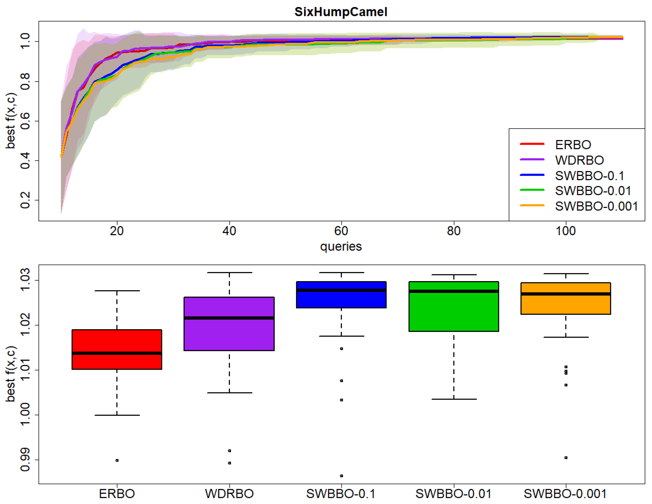
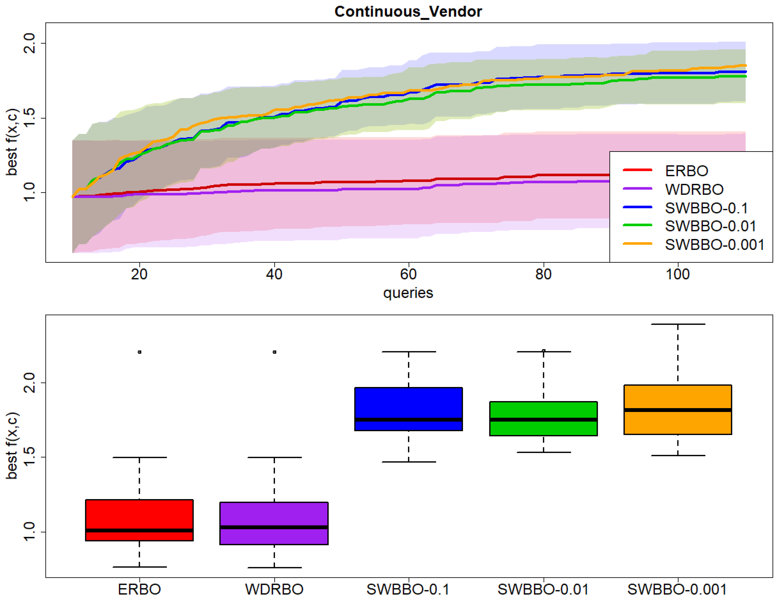
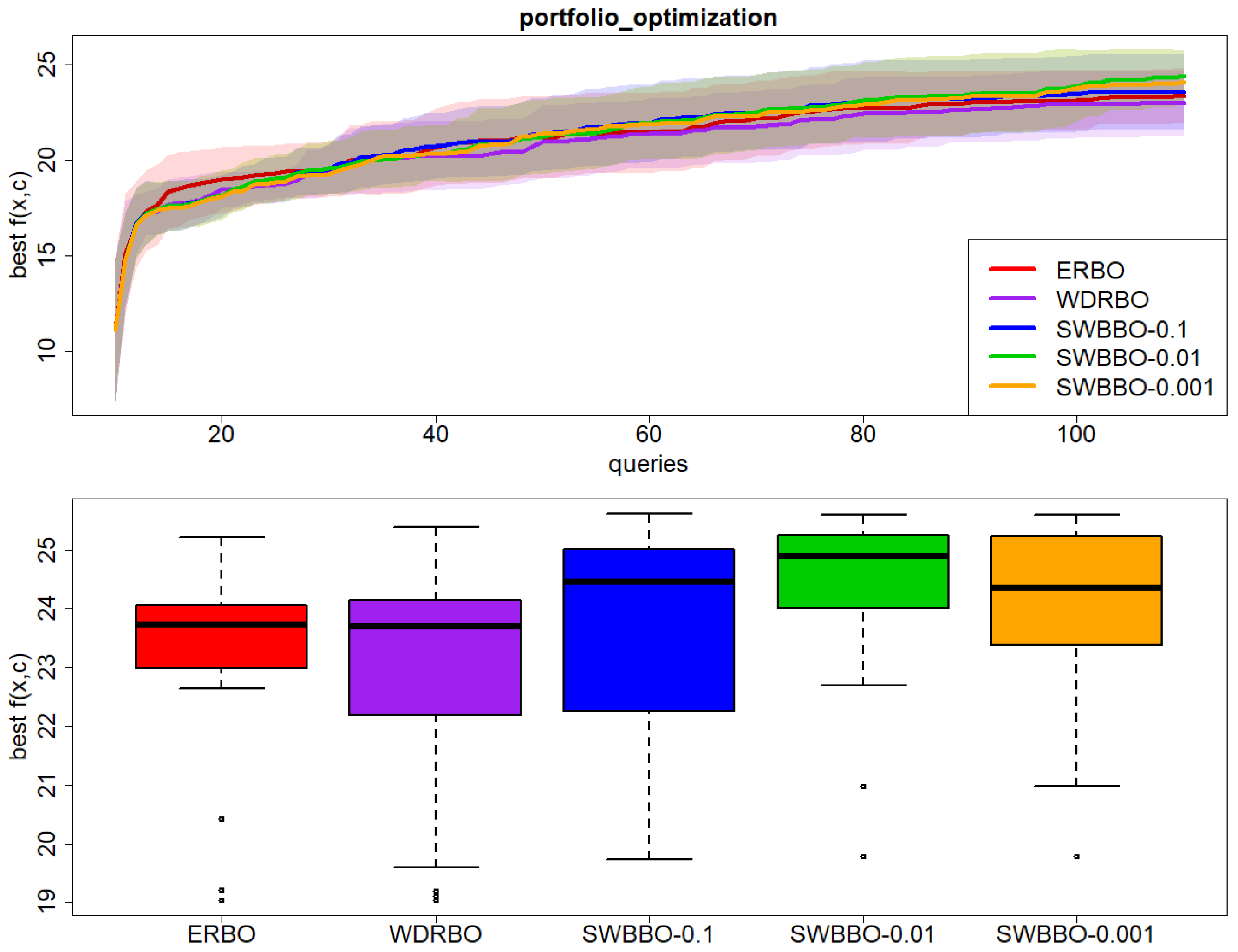
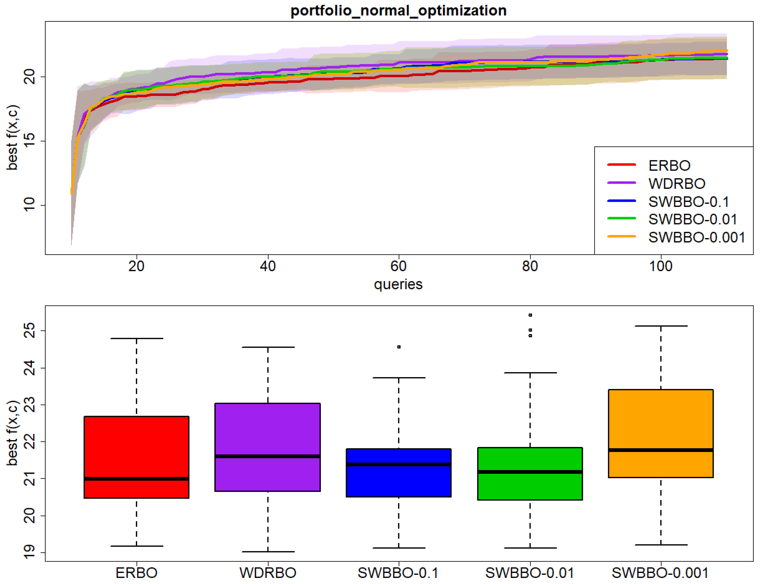
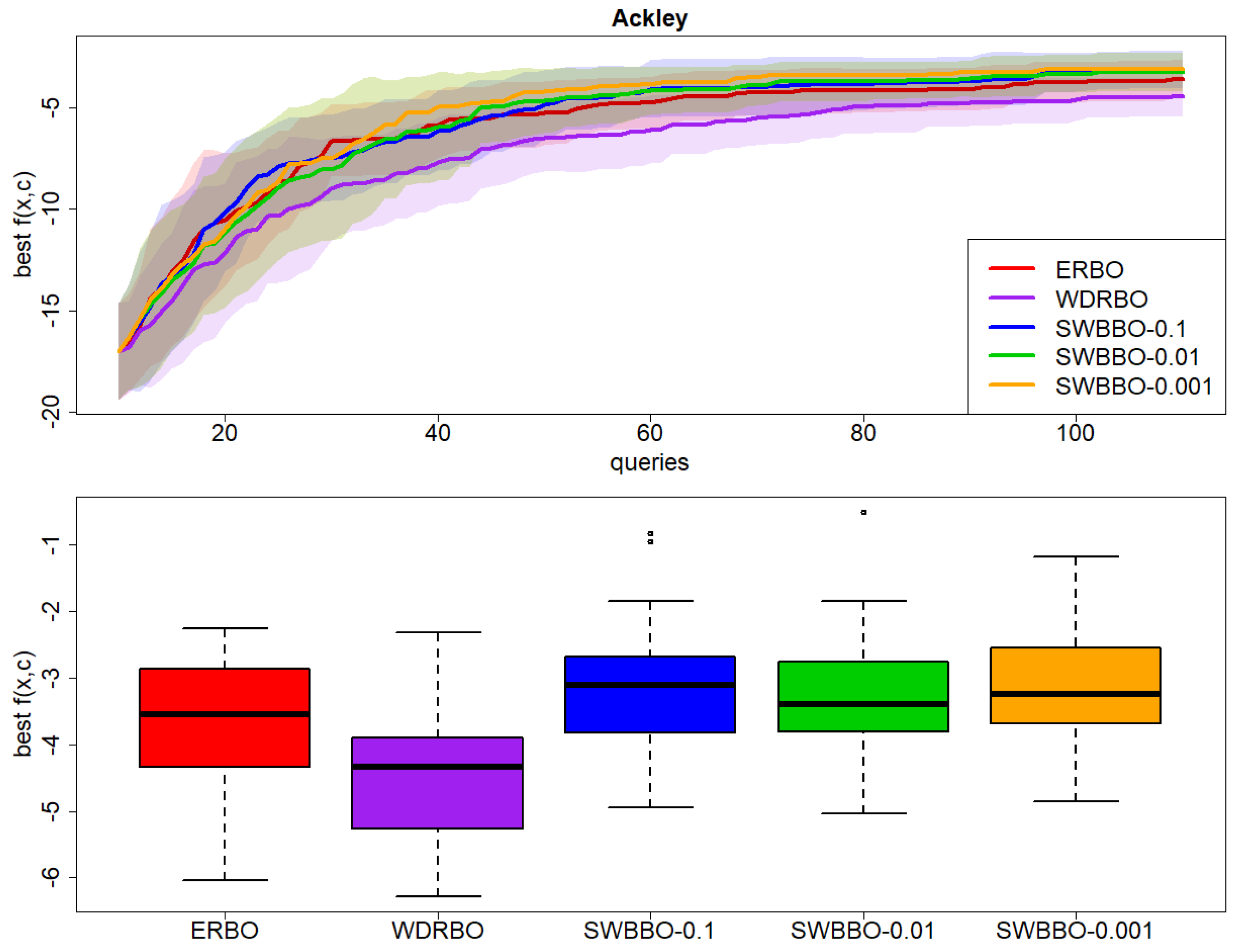
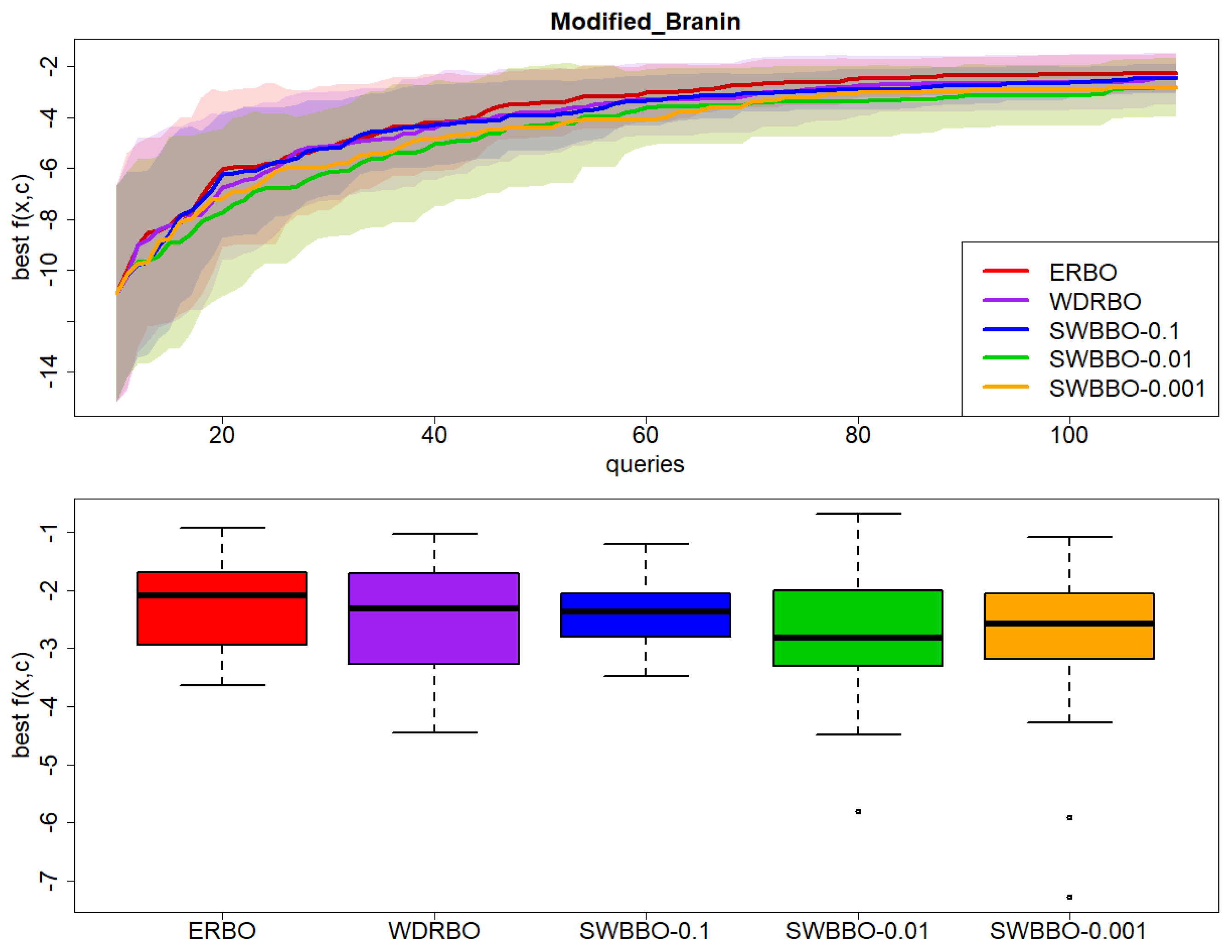
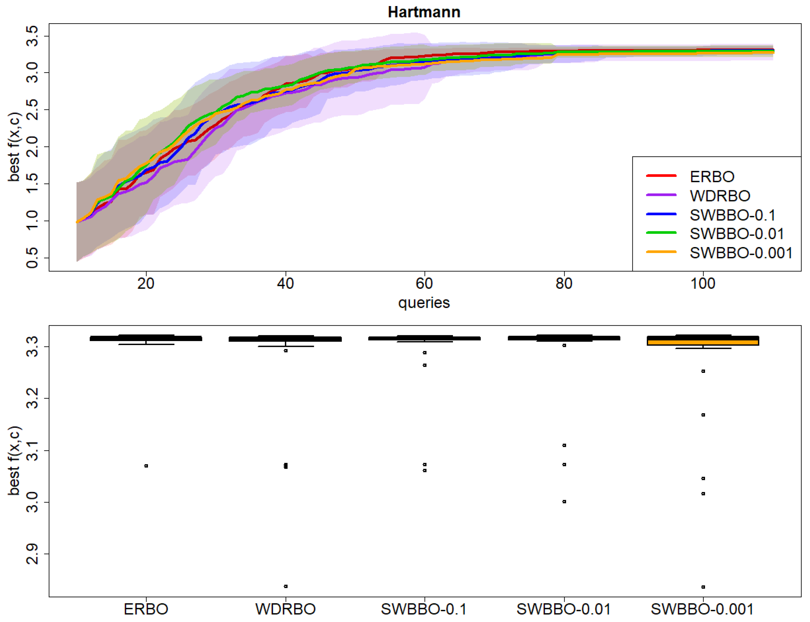
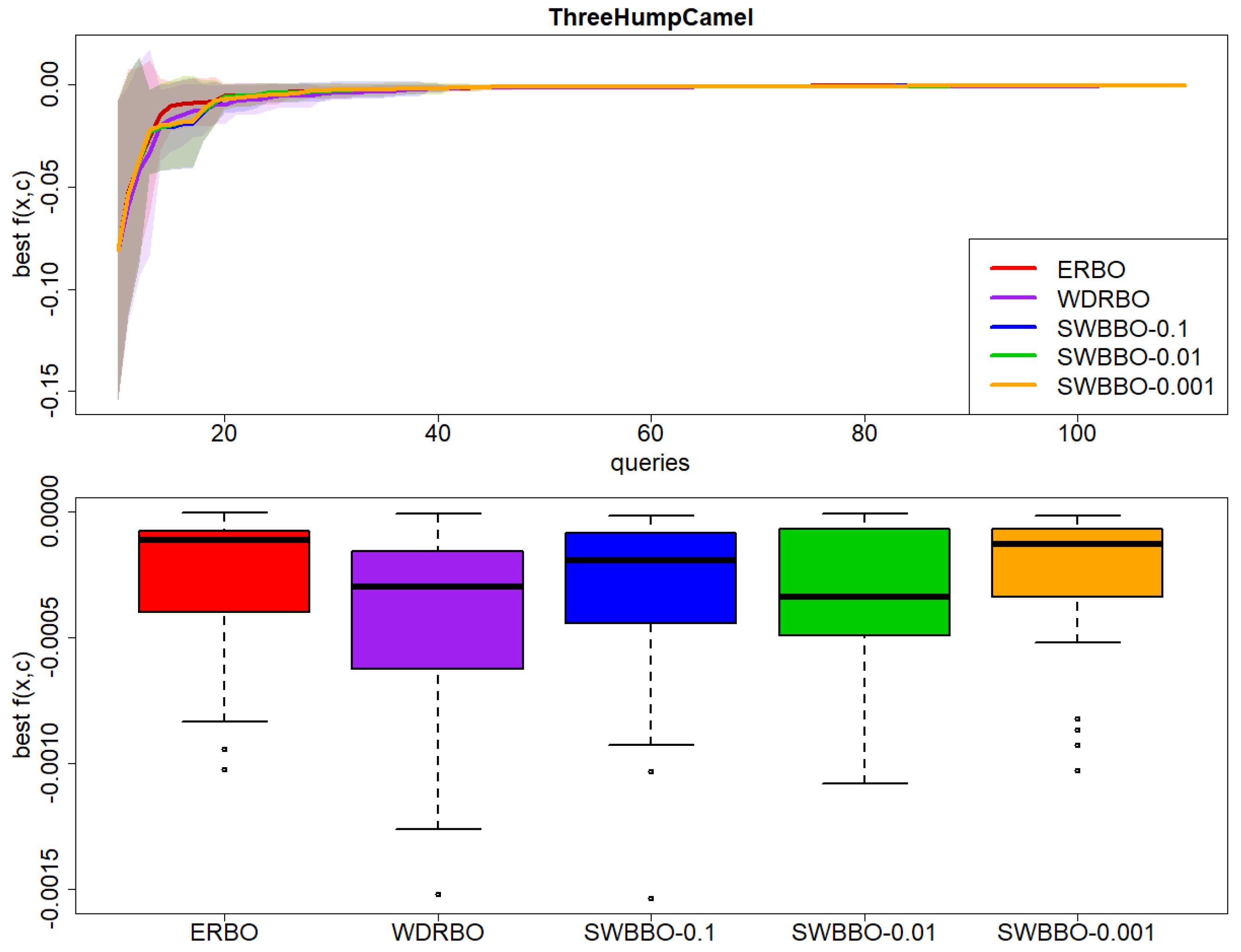
Following the experimental setting presented in Ref. [3], we have compared three DRBO algorithms on five benchmark test functions: Ackley, Modified Branin, Hartmann, Three Hump Camel, Six Hump Camel, and three real-life related problems, specifically, Continuous Vendor, Portfolio, and Portfolio Normal Optimization. The algorithms compared are Empirical Risk Bayesian Optimization (ERBO), Wasserstein Distance Robust Bayesian Optimization (WDRBO), and SWBBO (With $\gamma$ = 0.1, 0.01, 0.001). Each algorithm is evaluated over 30 independent runs to ensure statistical significance. The baseline methods, ERBO and WDRBO, are from the implementation provided by the authors of Ref. [9] as freely accessible on their GitHub repository.

The following table summarizes the best value of $f(x,c)$ observed at the end of the optimization processes performed by the different algorithms (median and standard deviation over 30 independent runs), separately for the test problems.

As reported in Ref. [9], ERBO is always better (on median) than WDRBO, apart from in the case of Portfolio Normal Optimization. Moreover, in our experiments—which are more extensive than those reported in Ref. [9]—this difference was statistically significant (with respect to a Wilcoxon test) in the following cases: Ackley (p-value = 0.001), Three Hump Camel (p-value = 0.046), and Six Hump Camel (p-value = 0.015), while it was not statistically significant in the following: Modified_Branin (p-value = 0.532), Hartmann (p-value = 0.260), Continuous Vendor (p-value = 0.605), Portfolio Optimization (p-value = 0.665), and Portfolio Normal Optimization (p-value = 0.254).

When ERBO is compared against the best among the three SWBBO alternatives (

Table 1. Best observed value of $\mathrm{f}(\mathrm{x},\mathrm{c})$ at the end of the optimization: median and (standard deviation) over 30 independent runs.

	ERBO	WDRBO	SWBBO $\mathit{\gamma }$ = 0.1	SWBBO $\mathit{\gamma }$ = 0.01	SWBBO $\mathit{\gamma }$ = 0.001
Ackley	−3.6299 (0.9521)	−4.4796 (0.9650)	−3.1460 (0.9238)	−3.2748 (0.9356)	−3.1267 (0.9036)
Modified_Branin	−2.2648 (0.7371)	−2.4816 (1.0053)	−2.4422 (0.5570)	−2.8250 (1.1473)	−2.5814 (1.2763)
Hartmann	−2.2648 (0.7371)	−2.4816 (1.0053)	−2.4422 (0.5570)	−2.8250 (1.1473)	−2.5814 (1.2763)
Three Hump Camel	3.3068 (0.0451)	3.2740 (0.1113)	3.2969 (0.0634)	3.2909 (0.0793)	3.2735 (0.1121)
Six Hump Camel	−0.0003 (0.0003)	−0.0004 (0.0004)	−0.0003 (0.0003)	−0.0003 (0.0003)	−0.0003 (0.0003)
Continuous_Vendor	1.0141 (0.0078)	1.0186 (0.0108)	1.0242 (0.0098)	1.0235 (0.0088)	1.0235 (0.0094)
Portfolio	1.1213 (0.2880)	1.1020 (0.2988)	1.8119 (0.2000)	1.7784 (0.1794)	1.8518 (0.2247)
Portfolio_normal	23.3439 (1.4309)	22.9966 (1.7259)	23.5711 (1.9742)	24.4015 (1.3356)	24.0899 (1.4707)

), its results are better (on median) only in the case of Modified Branin, but this difference is not statistically significant (p-value = 0.290). In all the other test problems, the best SWBBO alternative is (on median) better than ERBO; more precisely, it is significantly better in the following: Six Hump Camel (p-value < 0.001), Continuous Vendor (p-value < 0.001), and Portfolio Optimization (p-value < 0.001), while the difference is not statistically significant in Ackley (p-value = 0.127), Hartmann (p-value = 0.708), Three Hump Camel (p-value = 0.440), and Portfolio Optimization (p-value = 0.088). Results are also reported in Figure 4, Figure 5, Figure 6, Figure 7, Figure 8, Figure 9, Figure 10 and Figure 11.

Figure 4. Results on Ackley over 30 independent runs: (top) best observed value of $\mathrm{f}(\mathrm{x},\mathrm{c})$ with respect to BO queries and (bottom) boxplot of the final best value of $\mathrm{f}(\mathrm{x},\mathrm{c})$.

Figure 4. Results on Ackley over 30 independent runs: (top) best observed value of $\mathrm{f}(\mathrm{x},\mathrm{c})$ with respect to BO queries and (bottom) boxplot of the final best value of $\mathrm{f}(\mathrm{x},\mathrm{c})$.

Figure 5. Results on Modified_Branin over 30 independent runs: (top) best observed value of $\mathrm{f}(\mathrm{x},\mathrm{c})$ with respect to BO queries and (bottom) boxplot of the final best value of $\mathrm{f}(\mathrm{x},\mathrm{c})$.

Figure 5. Results on Modified_Branin over 30 independent runs: (top) best observed value of $\mathrm{f}(\mathrm{x},\mathrm{c})$ with respect to BO queries and (bottom) boxplot of the final best value of $\mathrm{f}(\mathrm{x},\mathrm{c})$.

Figure 6. Results on Hartmann over 30 independent runs: (top) best observed value of $\mathrm{f}(\mathrm{x},\mathrm{c})$ with respect to BO queries and (bottom) boxplot of the final best value of $\mathrm{f}(\mathrm{x},\mathrm{c})$.

Figure 6. Results on Hartmann over 30 independent runs: (top) best observed value of $\mathrm{f}(\mathrm{x},\mathrm{c})$ with respect to BO queries and (bottom) boxplot of the final best value of $\mathrm{f}(\mathrm{x},\mathrm{c})$.

Figure 7. Results on Three Hump Camel over 30 independent runs: (top) best observed value of $\mathrm{f}(\mathrm{x},\mathrm{c})$ with respect to BO queries and (bottom) boxplot of the final best value of $\mathrm{f}(\mathrm{x},\mathrm{c})$.

Figure 7. Results on Three Hump Camel over 30 independent runs: (top) best observed value of $\mathrm{f}(\mathrm{x},\mathrm{c})$ with respect to BO queries and (bottom) boxplot of the final best value of $\mathrm{f}(\mathrm{x},\mathrm{c})$.

Figure 8. Results on Six Hump Camel over 30 independent runs: (top) best observed value of $\mathrm{f}(\mathrm{x},\mathrm{c})$ with respect to BO queries and (bottom) boxplot of the final best value of $\mathrm{f}(\mathrm{x},\mathrm{c})$.

Figure 8. Results on Six Hump Camel over 30 independent runs: (top) best observed value of $\mathrm{f}(\mathrm{x},\mathrm{c})$ with respect to BO queries and (bottom) boxplot of the final best value of $\mathrm{f}(\mathrm{x},\mathrm{c})$.

Figure 9. Results on Continuous_Vendor over 30 independent runs: (top) best observed value of $\mathrm{f}(\mathrm{x},\mathrm{c})$ with respect to BO queries and (bottom) boxplot of the final best value of $\mathrm{f}(\mathrm{x},\mathrm{c})$.

Figure 9. Results on Continuous_Vendor over 30 independent runs: (top) best observed value of $\mathrm{f}(\mathrm{x},\mathrm{c})$ with respect to BO queries and (bottom) boxplot of the final best value of $\mathrm{f}(\mathrm{x},\mathrm{c})$.

Figure 10. Results on Portfolio_Optimization over 30 independent runs: (top) best observed value of $\mathrm{f}(\mathrm{x},\mathrm{c})$ with respect to BO queries and (bottom) boxplot of the final best value of $\mathrm{f}(\mathrm{x},\mathrm{c})$.

Figure 10. Results on Portfolio_Optimization over 30 independent runs: (top) best observed value of $\mathrm{f}(\mathrm{x},\mathrm{c})$ with respect to BO queries and (bottom) boxplot of the final best value of $\mathrm{f}(\mathrm{x},\mathrm{c})$.

Figure 11. Results on Portfolio_Normal_Optimization over 30 independent runs: (top) best observed value of $\mathrm{f}(\mathrm{x},\mathrm{c})$ with respect to BO queries and (bottom) boxplot of the final best value of $\mathrm{f}(\mathrm{x},\mathrm{c})$.

Figure 11. Results on Portfolio_Normal_Optimization over 30 independent runs: (top) best observed value of $\mathrm{f}(\mathrm{x},\mathrm{c})$ with respect to BO queries and (bottom) boxplot of the final best value of $\mathrm{f}(\mathrm{x},\mathrm{c})$.

Finally,

Table 2. Cumulative Stochastic Regret (CSR) and computational time: median and (standard deviation) on 30 independent runs.

	ERBO		WDRBO		SWBBO1		SWBBO2		SWBBO3
	CSR	Time	CSR	Time	CSR	Time	CSR	Time	CSR	Time
Ackley	329.37 (40.99)	192.78 (35.5)	477.969 (54.21)	142.11 (18.3)	221.232 (25.989)	101.66  (10.2)	215.007 (42.56)	239.08 (63.7)	217.558 (31.23)	178.28 (81.89)
Modified_Branin	847.91 (153.5)	114.50 (23.5)	909.500 (160.32)	98.704 (20.6)	913.623 (177.59)	113.17 (10.9)	1411.67 (330.3)	276.05 (66.4)	1300.74 (312.1)	174.34 (82.34)
Hartmann	53.4273 (11.62)	176.45 (19.1)	58.9245 (19.395)	196.57 (25.99)	52.3729 (25.716)	176.19  (33.97)	54.9945 (38.994)	319.52 (165.0)	53.2995 (47.91)	239.63 (156.4)
Three Hump Camel	4.8008 (0.6641)	205.87 (34.91)	4.9377 (0.6990)	244.91 (50.62)	4.8738 (0.7061)	101.93  (11.76)	4.9080 (0.6867)	112.18 (13.56)	5.0666 (0.7160)	161.29 (73.60)
Six Hump Camel	135.199 (49.428)	121.96 (15.64)	142.203 (50.576)	126.97 (22.99)	162.483 (51.242)	110.29 (13.47)	166.402 (67.497)	114.83 (14.70)	173.509 (84.057)	88.930  (8.576)
Continuous_Vendor	13.0761 (1.6257)	90.267  (12.90)	14.3611 (1.5091)	100.67 (12.27)	59.9870 (11.795)	111.64 (13.74)	63.1201 (11.191)	104.04 (12.14)	76.4769 (19.224)	94.936 (10.22)
Portfolio	436.454 (63.871)	191.84 (30.01)	436.660 (70.312)	206.12 (33.78)	479.525 (47.024)	171.26  (20.65)	493.743 (38.103)	187.76 (19.20)	484.731 (37.243)	207.32 (31.35)
Portfolio_normal	595.509 (80.1849)	186.44 (25.100)	573.669 (72.0094)	189.62 (23.748)	646.748 (63.9574)	176.69 (26.136)	669.314 (58.4004)	184.69 (25.934)	695.958 (62.4598)	145.18  (12.555)

summarizes the results related to the Cumulative Stochastic Regret (CSR) and computational time. It is evident that ERBO offered a lower CSR, on median, more frequently than the other methods, even in cases in which SWBBO has provided a better value of $f\left(x,c\right)$. The main plausible reason is a more explorative behaviour of SWBBO after the identification of its own best observed $f\left(x,c\right)$.

As far as computational time is concerned, there are no relevant differences between the approaches, nor is there an evident relationship between CSR and time. As shown in Table 2, SWBBO1 and SWBBO3 are often faster or comparable to baseline methods. SWBBO2, which uses a moderate regularization value, incurs slightly higher cost in some cases but offers improved robustness. Thus, computational trade-offs depend on the specific configuration and should be considered jointly with regret performance.

5.1. Evaluation Metrics

To evaluate how well our computed barycenters and transport maps perform, we use two established metrics from the entropic optimal transport literature [46]. The ${\mathrm{B}\mathrm{W}}_2^2-\mathrm{U}\mathrm{V}\mathrm{P}$ (Bures–Wasserstein Unexplained Variance Percentage) metric measures the quality of the generated barycenter compared to the ground truth, and it is defined as

$${\mathrm{B}\mathrm{W}}_2^2-\mathrm{U}\mathrm{V}\mathrm{P}\left(\nu , \tilde{\nu }\right)=100.{\displaystyle \frac{{BW}_2^2\left(\nu , \tilde{\nu }\right)}{\frac{1}{2}Var\left(\tilde{\nu }\right)}}\%,$$

(28)

where the Bures–Wasserstein metric is ${\mathrm{B}\mathrm{W}}_2^2\left(\nu , \tilde{\nu }\right)={\mathrm{W}}_2^2(\mathcal{N}\left({\mathrm{m}}_{\nu },{\mathsf{\Sigma }}_{\nu }\right),\mathcal{N}({\mathrm{m}}_{\tilde{\nu }},{\mathsf{\Sigma }}_{\tilde{\nu }})$, for the respective means and covariances of the distributions. This metric provides a normalized measure of the distance between the computed and true barycenter, expressed as a percentage of the target distribution’s variance. Where the Bures–Wasserstein metric is computed for the respective means and covariances of the distributions. The $L^2-UVP$ ($L^2$ Unexplained Variance Percentage metric assesses the quality of individual transport maps from each marginal distribution to the barycenter:

$$L^2-UVP(\widehat{T},T*)=100.{\displaystyle \frac{{‖\widehat{T}-T*‖}^2}{Var\left(\tilde{\nu }\right)}}$$

(29)

where $\widehat{T}$ denotes the learned transport map from the marginal to the barycenter, and $T*$ represents the ground truth mapping. This metric captures how well the learned transport maps approximate the optimal transport plans, normalized by the variance of the target distribution.

For illustration, we compute these metrics for the Ackley function across different regularization parameter values. The results demonstrate how regularization strength affects both barycenter quality and transport map accuracy.

Table 3. ${\mathrm{B}\mathrm{W}}_2^2-\mathrm{U}\mathrm{V}\mathrm{P}$ and $L^2-UVP$ metrics for the Ackley test problem.

Metric	$\mathit{\gamma }$	Ackley
	0.1	0.3542
${\mathrm{B}\mathrm{W}}_2^2-\mathrm{U}\mathrm{V}\mathrm{P}\mathrm{\%}$	0.01	0.7747
	0.001	0.0000
	0.1	7.1934
$L^2-UVP\mathrm{\%}$	0.01	7.8164
	0.001	7.5822

shows how well the barycenter computation and transport map estimation perform for the Ackley test function across different regularization parameter values (ε = 0.1, 0.01, 0.001), using two key evaluation metrics, ${\mathrm{B}\mathrm{W}}_2^2-\mathrm{U}\mathrm{V}\mathrm{P}$ and $L^2-UVP$. The ${\mathrm{B}\mathrm{W}}_2^2-\mathrm{U}\mathrm{V}\mathrm{P}$ metric shows that performance varies with regularization strength: moderate regularization ($\gamma$ = 0.1, 0.01) yields acceptable barycenter quality with ${\mathrm{B}\mathrm{W}}_2^2-\mathrm{U}\mathrm{V}\mathrm{P}$ values of 0.35% and 0.77% respectively, while strong regularization ($\gamma$ = 0.001) achieves perfect barycenter approximation with ${\mathrm{B}\mathrm{W}}_2^2-\mathrm{U}\mathrm{V}\mathrm{P}$ = 0.0000%. The $L^2-UVP$ metric values stay consistently around 7–8% across all regularization levels, which tells us that the learned transport maps maintain reasonable accuracy no matter which regularization parameter we choose. These results show that stronger regularization (smaller $\gamma$) improves barycenter quality for the Ackley function, while transport map fidelity stays stable. This suggests our method performs robustly across different regularization settings for this test problem.

5.2. Sinkhorn vs. LP Barycenter Comparison

Table 4. Comparison metrics between Sinkhorn Wasserstein and LP Barycenters for the Ackley test problem.

Metric	$\mathit{\gamma }$	Ackley
	0.1	0.002593
WD	0.01	0.001621
	0.001	0.001208
	0.1	0.010303
MED	0.01	0.007938
	0.001	0.003189
	0.1	0.000604
MMD	0.01	0.000299
	0.001	0.000059

shows a quantitative comparison between barycenters computed using the Sinkhorn Wasserstein method and those we obtained through Linear Programming (LP) for the Ackley test function across different regularization parameters (γ = 0.1, 0.01, 0.001). We use three metrics to evaluate them: Wasserstein Distance (WD), Mean Euclidean Distance (MED), and Maximum Mean Discrepancy (MMD). The results demonstrate that the regularization parameter has a significant impact on the agreement between Sinkhorn and LP Barycenters. For the Wasserstein Distance, the deviation decreases as regularization becomes stronger: from 0.002593 at $\gamma$ = 0.1 to 0.001621 at $\gamma$ = 0.01, and further to 0.001208 at $\gamma$ = 0.001. This pattern tells us that when we use smaller γ values, the two methods work much better together under optimal transport geometry. The Mean Euclidean Distance behaves the same way, dropping from 0.010303 when γ = 0.1 down to 0.007938 at γ = 0.01, and then down to 0.003189 at γ = 0.001. What this means is that the pointwise differences between the barycenters become much smaller when we use stronger regularization. The MMD Approximation, which measures distributional similarity through kernel-based comparison, shows the most dramatic improvement: from 0.000604 at γ = 0.1 to 0.000299 at γ = 0.01, and finally to 0.000059 at γ = 0.001.

Overall, the results show that both Sinkhorn and LP methods produce increasingly aligned barycenters as the regularization parameter becomes smaller, with the strongest agreement achieved at γ = 0.001 across all evaluation metrics for the Ackley function.

The ${\mathrm{B}\mathrm{W}}_2^2-\mathrm{U}\mathrm{V}\mathrm{P}$ and $L^2-UVP$ metrics might not really capture what is going on with entropic optimal transport convergence, since they are mainly looking at pointwise differences instead of the underlying geometric structure of how we compute Barycenters. The WD, MED, and MMD metrics seem like better choices for evaluation because they actually measure how well the distributions line up and whether the geometry stays consistent between different ways of computing Barycenters.

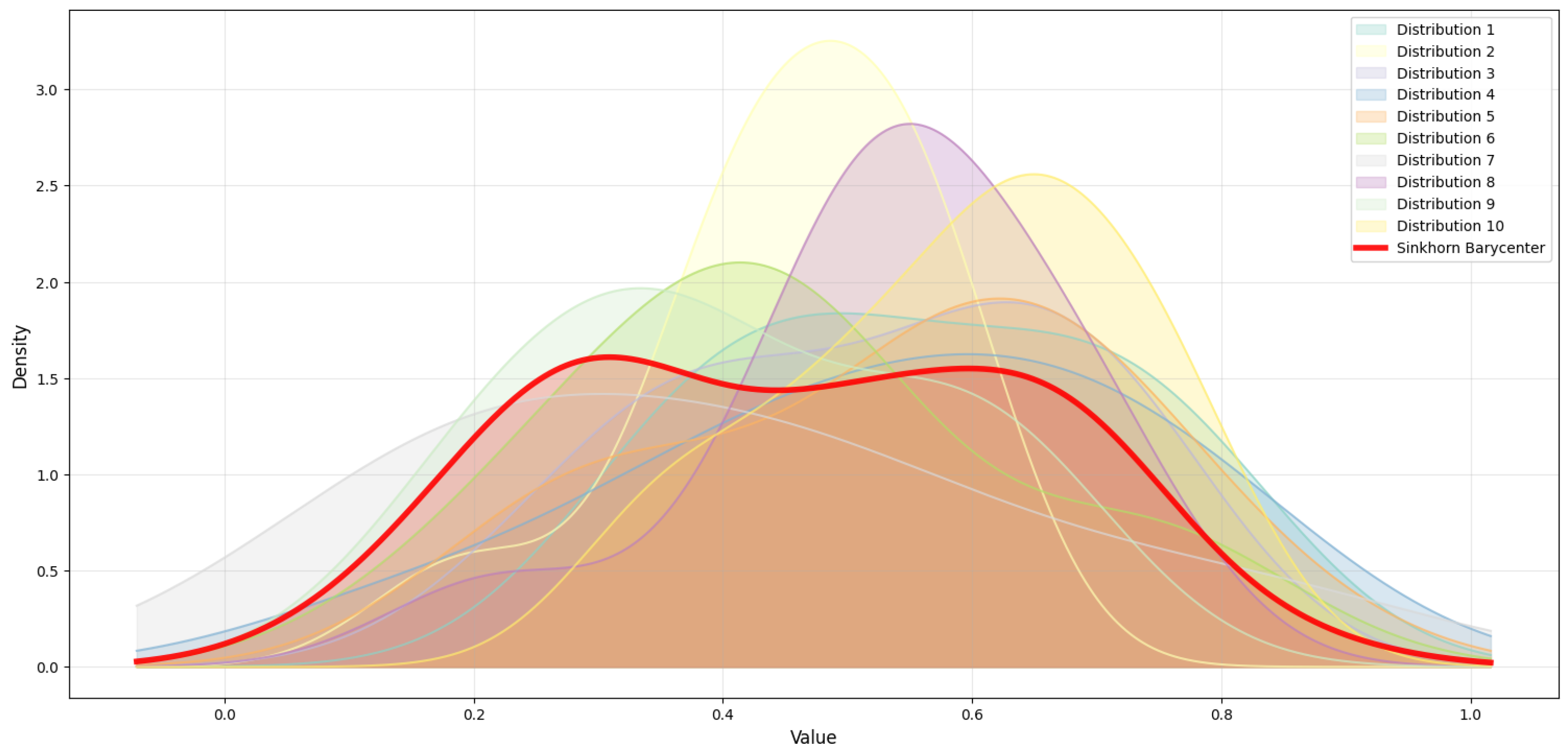
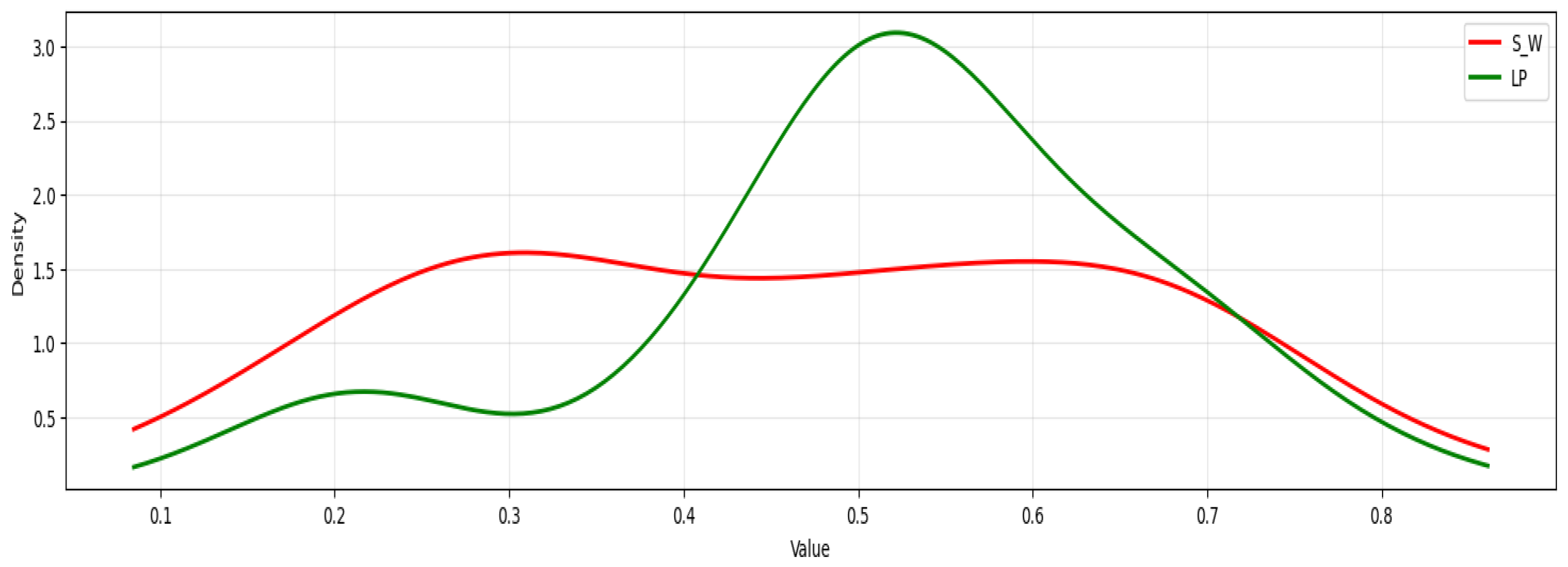
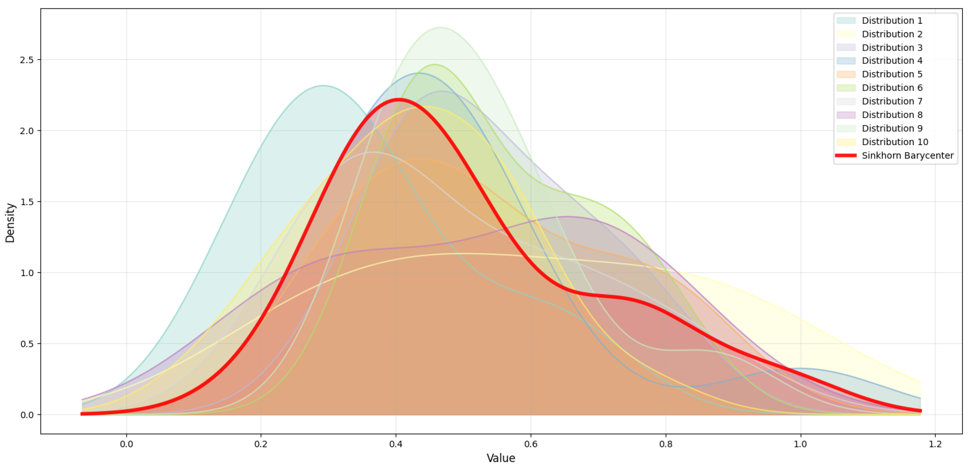
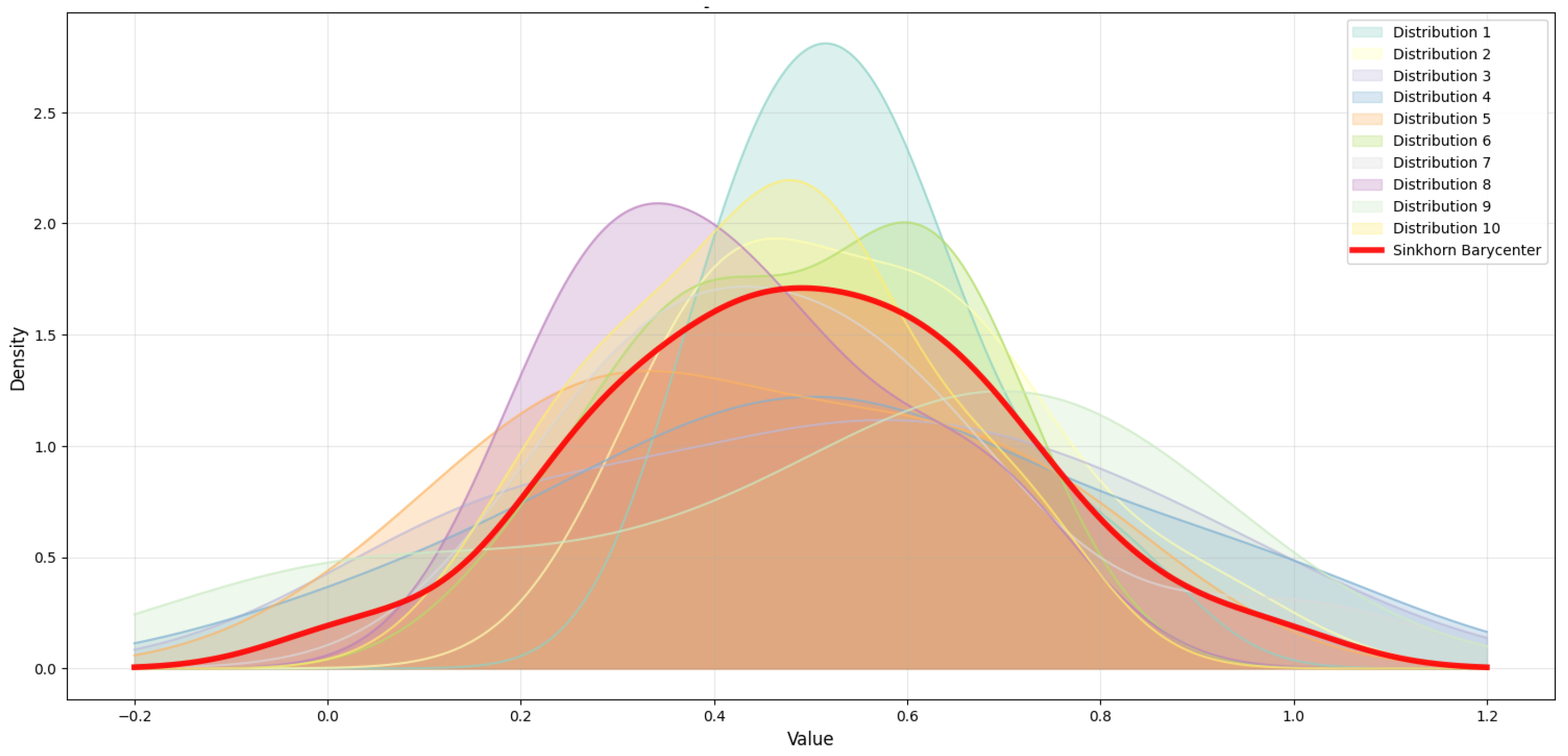
Figure 12, Figure 13, Figure 14, Figure 15, Figure 16 and Figure 17 show us a comparative analysis of Sinkhorn Barycenter computation versus LP Barycenter methods across different regularization strengths. We have organized the analysis in pairs, where the even-numbered Figure 12, and Figure 16 show the Sinkhorn Barycenter among multiple distributions with the computed barycenter highlighted in red, while the odd-numbered Figure 13, Figure 15 and Figure 17 give us direct comparisons between the Sinkhorn–Wasserstein (S-W) method (red curves) and LP method (green curves). The regularization parameter $\gamma$ decreases progressively across the figure pairs: Figure 12 and Figure 13 use $\gamma$ = 0.1, Figure 14 and Figure 15 use γ = 0.01, and Figure 16 and Figure 17 use γ = 0.001. This progression reveals the fundamental relationship between regularization strength and solution characteristics.

When we use high regularization (γ = 0.1, Figure 12 and Figure 13), the Sinkhorn method creates highly smooth, almost flat distributions that look quite different from what the LP solution gives us. The strong entropic regularization pushes the barycenter toward maximum entropy, which means we end up with broad, spread-out distributions. Meanwhile, the LP method keeps sharper, more concentrated peaks that do a better job of preserving what the original distributions actually looked like. When we move to moderate regularization (γ = 0.01, Figure 14 and Figure 15), the Sinkhorn Barycenter starts becoming closer to the LP solution while still staying smooth. The entropic regularization still smooths things out noticeably, but now the barycenter does a better job of capturing the underlying distribution structure with more defined peaks and valleys. At low regularization (γ = 0.001, Figure 16 and Figure 17), the Sinkhorn and LP methods converge toward nearly identical solutions. The minimal regularization lets the Sinkhorn method become really close to the true optimal transport solution while still keeping its computational advantages. The distributions show sharp, well-defined features that match up closely between both methods.

This progression shows us the trade-off between how fast we can compute things and how accurate our solution is in regularized optimal transport. When we use higher regularization, we obtain faster convergence, but we might end up smoothing out important features of the distributions too much. When we use lower regularization, we stay more faithful to the true barycenter, but it takes more computational work to achieve.

Figure 12. Sinkhorn Barycenter on Ackley at γ = 0.1.

Figure 12. Sinkhorn Barycenter on Ackley at γ = 0.1.

Figure 13. Sinkhorn vs. LP Barycenter comparison on Ackley at $\gamma$ = 0.1.

Figure 13. Sinkhorn vs. LP Barycenter comparison on Ackley at $\gamma$ = 0.1.

Figure 14. Sinkhorn Barycenter on Ackley at $\gamma$ = 0.01.

Figure 14. Sinkhorn Barycenter on Ackley at $\gamma$ = 0.01.

Figure 15. Sinkhorn vs. LP Barycenter comparison on Ackley at $\gamma$ = 0.01.

Figure 15. Sinkhorn vs. LP Barycenter comparison on Ackley at $\gamma$ = 0.01.

Figure 16. Sinkhorn Barycenter on Ackley at $\gamma$ = 0.001.

Figure 16. Sinkhorn Barycenter on Ackley at $\gamma$ = 0.001.

Figure 17. Sinkhorn vs. LP Barycenter comparison on Ackley at $\gamma$ = 0.001.

Figure 17. Sinkhorn vs. LP Barycenter comparison on Ackley at $\gamma$ = 0.001.

6. Conclusions: Limitations and Perspectives

BO works really well for optimizing data-driven systems when uncertainty is involved, where randomness comes from things like contextual conditions, model parameters, or noisy observations. In these situations, uncertainty has many different sides, which makes developing DRBO algorithms both important and tricky. One of the main challenges we face is that context distributions are infinite-dimensional, especially when we are dealing with continuous contexts. Solving BO problems robust to such uncertainty requires tractable approximations of otherwise intractable constrained optimization problems over probability spaces. Historically, robust BO formulations have employed φ-divergences to define ambiguity sets over context distributions. However, Wasserstein distances, arising from OT theory, have recently gained prominence due to their desirable geometric, topological, and statistical properties. Unlike φ-divergences, Wasserstein distances naturally incorporate the geometry of the underlying space and provide meaningful comparisons even when distributions have disjointed support. This geometry-aware notion of robustness allows the Wasserstein metric to capture subtle shifts in distribution and thus leads to better-behaved optimization landscapes. As a result, Wasserstein-based ambiguity sets have become increasingly popular for modeling uncertainty in robust machine learning, including BO.

Despite these advantages, computational complexity remains a well-known bottleneck. The exact computation of Wasserstein distances has a complexity of $O(n^3 log n)$ with respect to the number of samples n. This makes OT prohibitive in high dimensions. To address this, entropic regularization via the Sinkhorn algorithm has emerged as a practical alternative, offering a per-iteration complexity of $O\left(n^2\right)$. Moreover, Sliced Wasserstein approaches and neural OT methods (e.g., via learned transport maps) have enabled further scaling by approximating high-dimensional OT through lower-dimensional projections or learned parametrizations. The SWBBO algorithm developed in this study contributes to this growing intersection of Bayesian Optimization and optimal transport. By leveraging Wasserstein Barycenters, our methods offer tractable and robust BO strategies that adapt to distributional shifts in context while maintaining computational efficiency through entropic regularization. In conclusion, Wasserstein-based BO methods such as SWBBO offer promising tools for robust and geometry-aware optimization under uncertainty. While computational challenges remain, the flexibility and strong theoretical foundations of optimal transport provide a compelling framework for advancing robust machine learning, with exciting future applications in optimization, control, and learning under uncertainty.

Looking ahead, we expect this direction to keep expanding, especially when we integrate it with generative modeling, distributional Reinforcement Learning, and distributional robustness. In generative modeling, for example, people are increasingly using Wasserstein distances as loss functions because they can compare entire distributions rather than just point estimates. In dictionary learning, researchers use Wasserstein Barycenters to combine atoms meaningfully across distributional structures. Similarly, Distributional Reinforcement Learning expands what we are trying to learn from mean rewards to full return distributions, often using Wasserstein-based metrics for more informative policy updates.