1. Introduction
Quantum technologies have experienced remarkable growth in recent years. Since the mid-20th century, when Richard Feynman first introduced the concept of quantum computing, extensive research has been conducted in this field. Quantum computers leverage quantum mechanical principles such as superposition and entanglement. Unlike classical computers, which encode information using bits that represent either 0 or 1, quantum computers use qubits, which can represent both values simultaneously due to their quantum properties [
1].
Machine learning (ML) problems fundamentally involve two key tasks: efficiently managing large volumes of data and developing algorithms that process these data as quickly as possible. Quantum registers offer a significant advantage over classical registers in addressing the first task. While an
n-bit classical register can store only a single
n-bit binary string, an
n-qubit register can represent
n-bit binary strings simultaneously by encoding the information in quantum amplitudes. However, extracting all these strings is challenging, as measurement causes the quantum state to collapse, yielding only one string or amplitude as the output. Despite this limitation, qubits enable inherent parallelism, allowing algorithms to operate on all
strings simultaneously, which can lead to exponential speedups over their classical counterparts [
2].
Quantum algorithms are the foundation of quantum computing, with decades of research driving significant progress and breakthroughs. Among the nine key quantum algorithms—Deutsch’s algorithm, Deutsch–Josza algorithm, Bernstein–Vazirani algorithm, Simon’s algorithm, quantum Fourier transform, phase estimation algorithm, Shor’s algorithm, Grover’s algorithm and the HHL algorithm— Shor’s algorithm, introduced in 1994 [
3], was a major breakthrough, enabling the efficient factoring of large numbers—a problem believed to be computationally hard for classical computers, as no known polynomial-time classical algorithm exists for it. The algorithm leverages the quantum phase estimation (QPE) algorithm to estimate the eigenvalues of unitary operators [
4]. In 1996, Lov Grover further advanced the field with Grover’s algorithm [
5], achieving a quadratic speedup for searching unsorted databases.
Quantum machine learning (QML) is an interdisciplinary field that lies at the intersection of quantum computing (QC) and ML. The scope of this field leverages the principles of quantum mechanics to process and analyze data more efficiently. Due to the rapid growth of data, classical computers struggle to handle it effectively. As a result, QML presents a promising solution to address these challenges.
The progression of QML can be divided into two main stages. The first stage, from the mid-1990s to 2007, was mainly focused on the development of theoretical models. The second stage, which is ongoing, is concentrated on the practical application and implementation of these models [
6].
In 1995, Kak [
7] introduced a novel computational framework that integrates quantum mechanics with neural network models to enhance learning, memory, and processing efficiency. Building on this foundation, Ventura and Martinez proposed a quantum associative memory in 1999 [
8], capable of retrieving stored patterns exponentially faster than classical models. Around the same time, the concept of a qubit-like neuron was introduced [
9], followed by the proposal of a quantum neural network (QNN) [
10]. After these breakthrough proposals, other quantum machine learning techniques emerged, including the quantum support vector machine [
11] and the quantum k-means algorithm [
12].
The first comprehensive monograph on QML [
13] was published in 2014. This was followed by key implementations, including the first demonstration of a quantum neuron on a quantum processor as outlined in [
14]. In 2020, Google introduced Quantum TensorFlow [
15], seamlessly integrating quantum computing capabilities into the TensorFlow platform.
The aim of this work is to provide a tutorial for beginners to enter the field of QML by thoroughly studying the mathematics behind quantum algorithms and QML algorithms. Additionally, real-world applications are presented to illustrate the practical use of these concepts.
There are several review articles that present QML. What differentiates our work from previous studies is the following. In [
16], there is a comprehensive analysis covering both NISQ and fault-tolerant quantum algorithms. However, our study specifically focuses on fault-tolerant quantum algorithms and their mathematical preliminaries, which are missing in [
16]. While [
17] is a review on QML, it lacks a tutorial character, and quantum algorithms are not presented in detail. Our work, in contrast, provides a more structured and explanatory approach. In [
18], a review on QML is presented, but it does not include mathematical equations, which we explicitly cover in our study. In [
19], some quantum algorithms are presented in significant detail, but the article lacks a tutorial character and does not discuss possible applications in QML and QDL, which our study addresses. In [
20], the scope does not include an in-depth mathematical explanation of the algorithms, whereas our work aims to bridge this gap.
The paper is organized as follows:
Section 2 presents the fundamental theory of quantum computing. An analytic mathematical explanation of basic quantum algorithms is provided in
Section 3.
Section 4 and
Section 5 cover the fundamentals of quantum machine learning and quantum deep learning, respectively, along with some applications.
Section 6 highlights real-world applications of quantum machine learning. Finally, the conclusions are presented in
Section 7.
2. Overview of Quantum Computing
2.1. History and Evolution of QC
Quantum computing is an emerging field that leverages principles of quantum mechanics to perform computations. It sits at the intersection of mathematics, physics and computer science. While quantum computers exist today, their practical use remains minimal. Despite its immense potential, quantum computing is still in its early stages. Preskill [
21] first introduced the term “noisy intermediate-scale quantum (NISQ) era” because the current quantum circuits are susceptible to noise. However, there is optimism that NISQ-era devices will soon demonstrate practical applications, marking a significant step toward more advanced quantum computing.
The theoretical idea of quantum computing began in the mid-20th century and has since evolved into a rapidly advancing field of research and technological development. The development of quantum mechanics by physicists such as Niels Bohr, Werner Heisenberg, Erwin Schrödinger, and Paul Dirac in the 1920s and 1930s laid the groundwork for understanding the strange behavior of subatomic particles, such as superposition and entanglement—principles central to quantum computing. Einstein is considered the principal founder of quantum theory because he explained the photoelectric effect by proposing that light behaves as particles called quanta. The idea of quantum computing was introduced by Nobel laureate Richard Feynman. While working on a simulation for quantum physics models, he discovered that the values in his calculations were growing exponentially, requiring computational power far beyond what traditional computers could handle [
22].
Between 1980 and 2000, the foundational concepts of quantum computing emerged. In 1981, Richard Feynman proposed that a quantum computer could be used to simulate quantum systems, which classical computers could not perform efficiently. This is widely considered the first concrete proposal for a quantum computer [
22]. In 1985, David Deutsch, a British physicist, formalized the idea of a quantum Turing machine, a theoretical model for a universal quantum computer. His work demonstrated that a quantum computer could solve problems that classical computers could not. During the late 1980s, researchers began developing early quantum algorithms, including Deutsch’s algorithm. One of the most significant breakthroughs occurred in 1994 when Peter Shor developed an efficient quantum algorithm for integer factorization [
23].
In the early 2000s, researchers built small-scale quantum computers that could run simple algorithms. In 2001, researchers from IBM and Stanford University successfully implemented a small version of Shor’s algorithm on a 7-qubit quantum computer, factorizing the number 15. In 2011, D-Wave Systems, a Canadian company, launched its first commercial quantum computing system based on quantum annealing [
23].
After 2010, several companies began investing more heavily in the development of efficient quantum computers, aiming to build systems with a greater number of qubits. Nowadays, large companies such as Google, IBM and Microsoft, along with startups such as Rigetti, D-Wave, and Xanadu, have made breakthroughs in building quantum computers with increasing qubit capacities. Additionally, there has been active research in developing quantum algorithms and exploring the applications of quantum computers in real-world scenarios, including finance, machine learning, drug discovery and cryptography.
Quantum algorithms have been developed for both NISQ and fault-tolerant devices. For NISQ devices, the most important are variational algorithms, including the Variational Quantum Eigensolver (VQE) [
24], the Quantum Approximate Optimization Algorithm (QAOA) [
25] and Parameterized Quantum Circuits [
26].
A variational quantum circuit is a hybrid approach that combines quantum and classical computation, utilizing the advantages of both. It consists of a quantum circuit with adjustable parameters that a classical computer optimizes iteratively. These parameters function similarly to the weights in artificial neural networks [
27].
The algorithms described below refer to fault-tolerant quantum computing.
2.2. Bra–Ket Notation
States and operators in quantum mechanics are represented as vectors and matrices, respectively [
28]. Bra–Ket Notation, or Dirac notation, was introduced as an easier way to write quantum mechanical expressions.
A ket, denoted as
, represents a quantum state in a Hilbert space. It is a column vector that encapsulates all the information about the state of a quantum system. If
is a quantum state in a two-level system, it can be represented as
A bra is denoted as
. It is a row vector and is obtained by taking the conjugate transpose of a ket. If
is a quantum state, its corresponding bra is represented as
2.3. Quantum Bits
The fundamental component of QC is known as a quantum bit or qubit for short. Qubits are basic units of quantum information and function according to the principles of quantum mechanics. Quantum characteristics are not limited to subatomic particles, as larger systems can also exhibit quantum behavior. A qubit can be realized using various entities, including photons, electrons, neutrons, and even atoms [
29]. A qubit can be represented as a vector in a two-dimensional complex vector space. The states
and
are written in vector form as
A qubit can exist in a state of 0, a state of 1 or in a superposition of both states simultaneously, a phenomenon referred to as superposition. In contrast, classical bits are limited to a single value at any given time, either 0 or 1. Mathematically, a qubit can be expressed by the following equation:
where
is the qubit’s state and
and
represent the the probabilistic amplitude of the waveform of the state for being in the |0> state and |1> state, respectively. It must be noted that
Thus, the general state of a qubit
can also be written as
When we conduct a measurement, we retrieve a single bit of information, either 0 or 1. The simplest form of measurement occurs in the computational basis, represented by and . For instance, measuring the state on this basis yields a result of 0 with a probability of and a result of 1 with a probability of .
In quantum mechanics, the inner product between two vectors representing qubit states in a Hilbert space provides valuable information about their similarities. Specifically, the inner product is a mathematical operation that takes two quantum states, denoted as and and is represented as .
This inner product reveals important properties of the states:
1. Orthogonality: If the states
and
are orthogonal, meaning they are completely independent and share no information, the inner product equals zero:
Consequently, the inner product
can be computed as
2. Normalization: If the states are identical, that is
, the inner product equals one:
Consequently, the inner product
can be computed as
Quantum computing uses quantum physics principles including superposition and entanglement to process data. Superposition is described by Equation (
4). This property allows for the exponential speedup of quantum computing, as a qubit can exist in a combination of both states simultaneously. Quantum entanglement will be described in detail below.
2.4. Quantum Gates
The fundamental components of quantum circuits are quantum gates, which act on qubits. These quantum gates are realized through unitary operators, which serve to transform the state of a closed quantum system. Therefore, quantum gates are represented by unitary matrices. Unitary operators play a crucial role in evolving the quantum state, preserving the overall probabilities and maintaining the reversibility of the quantum process. The unitary operator maps the quantum state
into the state
as follows:
An operator
U is a unitary transformation if the following condition is satisfied:
where
is the conjugate transpose of the unitary operator
U, and
I is the identity operator.
The equation above describes the reversibility of a quantum system and ensures that the information contained in a quantum state can be recovered after the application of a quantum gate, allowing for the reconstruction of the original state prior to the operation. Every quantum gate operation is inherently reversible due to the unitary nature of quantum mechanics, unlike many classical operations.
Quantum gates operate on single-qubit, two-qubit or multi-qubit systems. Therefore, quantum gates can be categorized into three main categories: single-qubit gates, two-qubit gates and multi-qubit gates [
30]. Below is a concise representation of the most significant quantum gates in each category.
2.4.1. Single-Qubit Gates
Single-qubit gates operate on a single qubit. Common single-qubit gates are illustrated in
Figure 1 and include the following:
Pauli (X) Gate: Acts like a quantum NOT gate, flipping the state
to
and vice versa.
For example, applying the X gate to the state
,
Similarly, applying the X gate to the state
,
Pauli (Y) Gate: Introduces both a flip and a phase change.
For example, applying the Y gate to the state
,
Similarly, applying the Y gate to the state
,
Pauli (Z) Gate: Applies a phase flip to the
state.
For example, applying the Z gate to the state
,
Applying the Z gate to the state
,
Hadamard (H) Gate: It is one of the most frequently used quantum gates, transforming a basis state (
or
) into a superposition state.
For example, applying the H gate to the state
,
Similarly, applying the H gate to the state
,
2.4.2. Two-Qubit Gates
Two-qubit gates operate on two qubits simultaneously. A two-qubit system consists of two qubits, which together form a composite system. Each qubit can be in the state
or
, so the two-qubit system can be in one of four possible basis states:
The two-qubit system is described using the tensor product of the individual qubit states. If qubit 1 is in the state
and qubit 2 is in the state
, the combined state is
For example,
If
and
, then the combined state is
Common two-qubit gates include the following:
CNOT (Controlled-NOT) Gate: Flips the target qubit if the control qubit is
(
Figure 2a).
For example, applying the CNOT gate to the state
,
Similarly, applying the CNOT gate to the state
,
Similarly, applying the CNOT gate to the state
,
Finally, applying the CNOT gate to the state
,
The information above is summarized in the following
Table 1.
Table 1 shows that the output state of the target qubit corresponds to that of a standard XOR gate. The target qubit is
when both inputs are identical and
when the inputs differ.
SWAP Gate: Swaps the states of two qubits (
Figure 2b).
For example, applying the SWAP gate to the state
,
Similarly, applying the SWAP gate to the state
,
Similarly, applying the SWAP gate to the state
,
Finally, applying the SWAP gate to the state
,
The information above is summarized in the following
Table 2.
2.4.3. Multi-Qubit Gates
Multi-qubit gates operate on multiple qubits simultaneously. A multi-qubit system consists of
n qubits, which together form a composite quantum system. Each qubit can be in the state
or
, allowing the multi-qubit system to exist in one of
possible basis states. The states of the multi-qubit system are represented using the tensor product of the individual qubit states. If qubit 1 is in the state
, qubit 2 is in the state
and so on, the combined state of the system is given by
For example, if
,
, and
, then the combined state of the three-qubit system is
Fredkin Gate: Swaps the states of two target qubits based on the state of a control qubit. If the control qubit is
, the states of the two target qubits are swapped. If the control qubit is
, the target qubits remain unchanged (
Figure 3). The Fredkin gate is also known as the controlled-SWAP gate.
For example, applying the Fredkin gate to the state
,
Similarly, applying the Fredkin gate to the state
,
The information above is summarized in the following
Table 3.
2.5. Quantum Measurement
After the application of quantum gates, the measurement process is initiated. Measurement in quantum computing constitutes a fundamental concept that significantly influences the operation of quantum systems and their interaction with classical information. Following the execution of a series of quantum gates, the state of a quantum system can be represented by a quantum state vector
. This state vector encapsulates the information regarding the quantum system and can be expressed as a superposition of orthonormal basis states:
where
denotes the orthonormal basis states and
are the complex coefficients that characterize the probability amplitudes associated with each basis state. Upon measurement, the quantum state collapses to one of the possible basis states, with the probability of obtaining a particular state
given by the square of the magnitude of the corresponding coefficient [
31]:
The measurement process is essential, as it facilitates the extraction of information and enables decision-making based on the results of quantum computations.
2.6. Quantum Entanglement
An important principle of quantum computing is called entanglement, which has no classical analogue. Qubits can become entangled, a phenomenon in which the state of one qubit is directly related to the state of another, regardless of the distance between them [
32]. In simple terms, two quantum systems are entangled when their combined state cannot be written as tensor product of basic states.
Suppose that two qubits
and
are in the state
, which is given by
can also be written as
That is, the states of
and
are
Therefore,
can be written as
Specifically, can be written as the tensor product of the states of the two qubits, so that and are not in quantum entanglement but in a separable state.
Let us consider two other qubits,
and
, which are in the state
, given by
The state cannot be written as the tensor product of the states of the two qubits, so and are in quantum entanglement. The difference between separability and entanglement is explained as follows.
When qubit is measured in state , it is always found in . Afterward, qubit has a 50% chance of being in or , meaning ’s measurement does not affect . When qubit is measured in state , it has a 50% chance of being in or . If is found in , will be ; if in , will be . This shows that measuring one entangled qubit determines the state of the other.
Bell states are quantum states involving two qubits that represent the simplest form of quantum entanglement. The quantum circuit that creates Bell states is shown in
Figure 4. While there are various ways to generate entangled Bell states using quantum circuits, the most basic approach starts with a computational basis as the input and employs a Hadamard gate followed by a CNOT gate.
Suppose that the input state is given by the following equation:
Next, a Hadamard gate is applied to the q0 qubit, putting it into a superposition state using Equation (
23).
Then, q0 acts as a control input to the CNOT gate and the target qubit (q1) gets inverted only when the control is 1. The output is as follows:
Table 4 summarizes the results of the Bell state circuit computation. For example, knowing the state of two input qubits and measuring one of the output qubits allows us to determine the state of the other qubit, as the two qubits are entangled.
The expression
is a measurement of the degree of entanglement. The following equation shows whether two states, A and B, are completely separable or have some degree of entanglement:
Here, represents the trace of the square of a density matrix .
Two states are completely entangled when
The density matrix
can be computed by the following equation:
The reduced density matrix
can be computed by the following equation:
As an instance, consider the following Bell state:
The density matrix of qubit
A is given by
Considering that the basis states are orthogonal, we have
The corresponding density matrix is
Therefore,
can be computed as
The above computation indicates that the initial states are completely entangled.
As another example, the initial state of the two-qubit system is given by
The density matrix of qubit
A is given by
The corresponding density matrix is
Therefore,
can be computed as
The above computation indicates that the initial states are completely separable.
2.7. Quantum Computing Models
Quantum computing models provide abstract frameworks that define how quantum information is processed, specifying how qubits are manipulated and how computation proceeds in a quantum system. The quantum computing model described above is the quantum circuit model, also known as the gate-based model. This is the most widely used and familiar framework for quantum computing, analogous to classical digital circuits.
Figure 5 depicts the main idea of this model. The quantum circuit model consists of three stages: initialization of quantum gates, implementation of quantum gates, and measurement. This model serves as the foundation for most current quantum computers, including those developed by companies like IBM and Google.
However, several other models have also been proposed, such as the adiabatic model (used by D-Wave Systems) [
33], the topological model (explored by Microsoft) [
34], and the quantum annealing model (also used by D-Wave Systems) [
35].
2.8. Physical Representation of Quantum Computers
The physical representation of quantum computers encompasses a variety of methodologies, each with unique advantages and challenges. Ongoing research in these areas aims to optimize performance, enhance scalability and develop practical quantum computing systems. As the field progresses, these diverse approaches contribute to the broader goal of achieving functional and effective quantum computing technologies. The most important technologies that demonstrate quantum computers are
Ion Trap Quantum Computing. This method involves trapping individual ions using electromagnetic fields. The ions serve as qubits and their quantum states are manipulated using laser beams [
36].
Superconducting Quantum Computing. This approach involves circuits made from superconducting materials that exhibit quantum behavior at low temperatures. The qubits are manipulated using microwave pulses, allowing for fast and efficient operations [
37].
Linear Optical Quantum Computing. This method uses photons as qubits and leverages the properties of linear optical elements (like beam splitters, phase shifters, and detectors) to process quantum information [
38].
Semiconductor Spin-Based Quantum Computing. This approach uses the spin states of electrons in semiconductor materials (like silicon) as qubits. Spin qubits can be created using quantum dots or by doping silicon with specific atoms [
36].
Nuclear Magnetic Resonance (NMR)-Based Quantum Computing. NMR quantum computing employs the nuclear spins of molecules as qubits. Magnetic fields and radiofrequency pulses are used to manipulate the spins [
36]. It was the initial approach to building quantum computers, but it has since become less favored [
37].
Quantum Computing with Defects. This approach uses defects in solid-state materials (like nitrogen-vacancy centers in diamond or silicon vacancies in silicon carbide) as qubits [
38].
Several companies are actively working on the physical implementation of quantum computers using various approaches. For instance, IBM and Google are focusing on superconducting qubits, while IonQ is advancing the trapped ion approach. Xanadu is exploring linear optical quantum computing [
37]. These companies are making significant investments in quantum technology and frequently achieving new milestones, contributing to a clearer understanding of how these machines function. Their ongoing efforts are steadily advancing toward unlocking the true potential of quantum computers [
22].
2.9. Quantum Noise
Quantum noise refers to the inherent uncertainty and random fluctuations found in quantum systems as a result of quantum physics’ fundamental principles. Unlike classical noise, which is caused by external sources such as heat disturbances or electromagnetic interference, quantum noise inevitably arises from the fundamental features of quantum particles. This is the result of the Heisenberg Uncertainty Principle, which asserts that some pairs of physical quantities, such as position and momentum, cannot be correctly measured at the same time.
In quantum information science, quantum noise can produce decoherence, which occurs when quantum systems lose their unique quantum features and behave more like classical systems. This issue poses a major barrier to the creation of reliable quantum computers. To limit the influence of quantum noise, researchers use approaches like quantum error correction, which detect and correct noise-induced errors [
39].
3. Quantum Algorithms
As one group of researchers made progress on the physical implementation of quantum computers, others advanced in identifying algorithms that would run on a quantum computer with a speedup over classical computers.
Just as classical computers rely on classical algorithms for their functionality, quantum computers depend on quantum algorithms. These algorithms aim to demonstrate the advantages of quantum computing over classical computing. The investigation of quantum algorithms has constituted a dynamic area of research for over 20 years; however, the development of a fully operational quantum computer remains a work in progress [
40].
As previously mentioned, the quantum circuit model is the most widely utilized framework in quantum computing. Quantum algorithms are typically represented by quantum gates that operate on a set of qubits and conclude with a measurement process.
After proposing the concept of a quantum Turing machine, Deutsch [
41] developed an algorithm to demonstrate faster performance on a quantum computer. The Deutsch algorithm solves the problem of determining whether a function is constant or balanced using just one query, whereas a classical computer requires two queries. This algorithm showcases the strength of quantum parallelism. Deutsch, together with Richard Jozsa, later extended this idea into the more general Deutsch–Jozsa algorithm [
42].
In 1993, Bernstein and his student Vazirani published a paper [
43] introducing an algorithm that outperforms the best-known classical approach to a specific problem. Furthermore, they contributed by presenting a quantum version of the Fourier transform within the same paper.
Following the contributions of Bernstein and Vazirani, Daniel Simon made further advancements in 1994. Simon presented a problem [
44] that could be solved exponentially faster by a quantum computer compared to a classical one.
One of the most important breakthroughs in quantum computing was Shor’s algorithm [
3], developed in 1994. Shor built on earlier work by Deutsch, the Bernstein–Vazirani algorithm and Simon’s algorithm to create a way to quickly factor large numbers into two prime factors. While classical computers find this task extremely hard, Shor’s algorithm can complete it efficiently on a quantum computer, thanks in part to the quantum phase estimation algorithm, which is essential for estimating the eigenvalues of the unitary operators involved in the computation. Factoring large numbers is fundamental for the Rivest–Shamir–Adleman (RSA) encryption system, which secures most online communication today. This includes protecting credit card info, bank transfers and private messages [
32].
Following Shor’s groundbreaking work, Lov Grover developed another significant quantum algorithm in 1996. His algorithm [
5] focuses on searching through an unsorted database and provides a substantial quadratic speedup compared to classical algorithms.
The last fundamental quantum algorithm proposed by Harrow, Hassidim and Lloyd is called HHL algorithm [
45]. This algorithm is designed to solve linear systems of equations and demonstrates the potential for exponential speedup under certain conditions compared to classical methods.
Table 5 contains all the aforementioned algorithms with a brief description of their function. These nine quantum algorithms are fault-tolerant.
3.1. Deutsch’s Algorithm
Deutsch’s algorithm was one of the first quantum algorithms to demonstrate that quantum computers could solve certain problems more efficiently than classical ones. Deutsch’s problem involves a black-box function,
, that takes a single bit as input and outputs a single bit. This algorithm is designed to determine whether function
is constant or balanced. A function
is classified as constant if the output is the same for both inputs (either always 0 or always 1) while it is classified as balanced if the output differs for each input (0 for one input, 1 for the other). This can be expressed mathematically as follows:
Before the mathematical representation of the algorithm, it is crucial to explain an important property known as the phase oracle property.
Figure 6 represents the quantum circuit of the phase oracle property.
Let
be a unitary operator that maps the state
to
. This can be expressed mathematically as follows:
where ⊕ denotes addition modulo 2 (XOR operation).
Set
. Then, the unitary operator
acts as follows:
since
and
.
The final state does not depend on the y state.
Set
=
. Thus, the operation of
becomes
Thus, let
be a unitary operator that maps the state
to
. This property is mathematically expressed as
The Deutsch–Jozsa algorithm can be implemented following a common five-step procedure. The quantum circuit for this algorithm is depicted in
Figure 7.
First, initial input states are set up.
Next, a Hadamard gate is applied to each qubit, putting it into a superposition state using Equations (
23) and (
24).
In the third step, an oracle operation is applied. Thus, using Equation (
76),
is expressed as follows:
In the fourth step, Hadamard gates are applied. Therefore,
Therefore, by measuring the first qubit, the function f can be determined to be either constant or balanced. If the measurement of the first qubit yields , then f is constant; if the measurement yields , then f is balanced.
A classical computer would require at least two evaluations, while a quantum computer requires only one. This algorithm is based on quantum parallelism and highlights the power of quantum computers. However, it does not have any practical applications.
3.2. Deutsch–Josza Algorithm
The Deutsch–Jozsa algorithm is a generalization of the Deutsch algorithm and it is designed to determine whether a given Boolean function
is constant or balanced. The Deutsch–Jozsa algorithm can be implemented following a common five-step procedure. The quantum circuit for this algorithm is depicted in
Figure 8.
First, initial input states are set up.
Next, a Hadamard gate is applied to each qubit, putting it into a superposition state.
With the help of Equation (
83),
can be expressed as
In the third step, an oracle operation is applied. Thus, using Equation (
76),
is expressed as follows:
In the fourth step, Hadamard gates are applied. Therefore,
For the measurement, the state
is not of interest.
Therefore,
is expressed as follows:
Finally, a measurement of the qubits is performed to obtain the answer.
The probability of measuring the
state is
If f is constant:
If f(x) = 0 for all x, then:
If f(x) = 1 for all x, then:
Amplitude of state is .
Thus, if the state is measured, then the function f is confirmed to be constant. Conversely, if any other state is measured, it indicates that f is balanced.
Some positive aspects of the Deutsch–Jozsa algorithm include its ability to provide an exponential speedup over classical algorithms for the specific problem it addresses. While a classical algorithm might require up to queries to the function to determine if it is constant or balanced, the Deutsch–Jozsa algorithm requires only one quantum query. However, the Deutsch–Jozsa algorithm solves a very specific problem, leading to its limited practical application. The Deutsch–Jozsa algorithm served as a foundational milestone for the advancement of more important quantum algorithms.
3.3. Bernstein–Vazirani Algorithm
The Bernstein–Vazirani algorithm is designed to determine an
n-bit “hidden string”
s by querying a function
, which is defined as
where
x is any
n-bit binary string, representing the input to the algorithm, and
denotes the bitwise dot product of
s and
x, calculated as
The Bernstein–Vazirani algorithm can be implemented following a common five-step procedure. The quantum circuit for this algorithm is depicted in
Figure 9. The quantum topology of this circuit is the same as that of the Deutsch–Josza algorithm.
First, initial input states are set up.
Next, a Hadamard gate is applied to each qubit, putting the system into a superposition state as described by Equations (
24) and (
83).
In the third step, an oracle operation is applied. Thus, using Equation (
76),
is expressed as follows:
For the measurement, the state is not of interest.
In the fourth step, Hadamard gates are applied. Therefore,
With the aim of Equation (
87),
can be expressed as
The term can be expressed as because
If
, the sum
evaluates to zero for all
. This is because
takes on an equal number of 0 and 1 values as
x varies over the
possible
n-bit strings, resulting in equal numbers of
and
terms, which sum to 0.
Thus,
can be expressed as
Finally, is measured to obtain the answer.
The amplitude of
is
The probability of measuring the state is 1.
The output of the Bernstein–Vazirani algorithm is the hidden bit string s, which is retrieved with just one query to the oracle, demonstrating the efficiency of QC over classical methods for this specific problem.
3.4. Simon’s Algorithm
Simon’s problem can be defined as follows:
A function
that maps bit strings to bit strings. The unknown function f maps either each unique input to a unique output or maps two distinct inputs to one unique output. In mathematical terms, this can be expressed as
for some
. The goal is to determine whether f is one-to-one or two-to-one by finding the hidden string
s with as few evaluations of
f as possible.
In order to solve this problem, a classical approach requires queries, while Simon’s algorithm promises to solve this using n queries.
Simon’s Algorithm Example:
Consider the function
defined by the truth
Table 6.
Each output
appears twice for two distinct inputs. For example,
Simon’s algorithm can be implemented following a common five-step procedure. The quantum circuit for this algorithm is depicted in
Figure 10.
First, initial input states are set up.
Next, a Hadamard gate is applied to each qubit, putting them into a superposition state.
In the third step, an oracle operation is applied. Thus,
is expressed as follows:
The output of f corresponds to an input of either x or y where x and y are two different inputs to f that gave the same output. Hence, the n bits are in the state
In the fourth step, Hadamard gates are applied. Therefore,
Using Equation (
87),
is expressed as follows:
Finally, a measurement of the qubits is performed to obtain the answer. The measurement returns a random bit string
z such that
Thus, the bit string z is orthogonal to the secret string s.
From the measurement results
, a system of equations is formed such that
There are k equations and n unknowns. The secret string s can be solved by solving the system of equations derived above.
Simon’s algorithm demonstrates the power of quantum algorithms. while the best classical algorithms for the same problem may require exponential time, Simon’s algorithm can solve it in polynomial time.
3.5. Quantum Fourier Transform
The quantum Fourier transform, or QFT for short, transforms a qubit from the computational basis
to the Fourier basis
. Although the QFT does not speed up the classical task of computing Fourier transforms of classical data [
39], it is an important component of the quantum phase estimation algorithm, which will be explained in detail later.
Consider the computational basis
(in decimal notation) with
, where
n is the number of qubits. The action of the QFT on a basis state
is given by
Any quantum state
can be written as a linear combination of the basis states. Therefore, QFT acts on a general quantum state
as follows:
where .
The matrix representation of QFT is as follows:
where .
Another representation of the QFT is described by the following equation:
The above equation can be summarized as
The above representation has adopted the notation
to represent the binary fraction
. The quantum circuit for this algorithm is depicted in
Figure 11. Each qubit went from
to
.
The QFT consists of two types of quantum gates: the Hadamard gate and the controlled
gate. If a Hadamard gate is applied to any
, the result will be as follows, in accordance with Equations (
23) and (
24):
This can be generalized by the following expression:
Because the term is equal to if and if .
The controlled
gate is described mathematically using the following equation:
For example, applying the
gate to the state
, where the first qubit indicates the control qubit while the second qubit indicates the target,
Similarly, applying the
gate to the state
,
Similarly, applying the
gate to the state
,
Finally, applying the
gate to the state
,
This gate applies a phase of for the state on the target qubit and acts only if the control qubit is in the state .
The action of
on a two-qubit state
where the first qubit is the control and the second is the target is given by
In the quantum circuit design for the QFT, the following gates are required:
For the first line, only 1 Hadamard gate is required.
For the second line, there are 1 Hadamard gate and R gates.
For the line, we need 1 Hadamard gate and 1 R gate.
Additionally, there are swap gates.
To summarize, the total number of quantum gates required can be calculated as follows:
where n represents the number of qubits in the system.
In terms of complexity, QFT requires operations while the classical Fourier transform requires . Therefore, QFT demonstrates superior performance in terms of complexity.
Let us present a simple example of a 3-qubit system and calculate the QFT of number 5.
Figure 12 represents this circuit.
The binary representation of the number 5 is 101. Since qubits in Qiskit are initialized in the state, the first and third qubits should have an X gate applied to initialize them in the state. Next, Hadamard gates are applied to every qubit. Sequentially, UROT gates are applied. Finally, swap gates are used to reverse the order of the qubits.
Generally, the number can be represented in the binary system as .
Firstly, the Hadamard gate is applied to
. The output is as follows:
Next, the
gate is applied using Equation (
128):
Next, the
gate is applied using Equation (
128):
In the next step, a similar process is applied to
.
Next, the
gate is applied using Equation (
128):
Finally, a similar process is applied to
.
The output is as follows:
Finally, a swap gate is applied:
Therefore, the number 5 can be represented by QFT by the following:
In addition to the QFT, there is also the inverse IQFT. Mathematically, this is described as follows. If
is the result of the application of the QFT algorithm to
,
The result of the inverse QFT is as follows:
Although the QFT requires fewer operations in comparison with the classical Fourier transform, practical implementations of QFT are limited. The QFT’s exponential speedup in certain quantum algorithms, such as quantum phase estimation and Shor’s algorithm, demonstrates its significance in quantum computing.
3.6. Quantum Phase Estimation
Quantum phase estimation is a key subroutine for important quantum algorithms, including Shor’s algorithm. Suppose a unitary operator
U has an eigenvector
with eigenvalue
, where the value of
is unknown [
39]. The goal of the phase estimation algorithm is to estimate
. This can be expressed mathematically using the following equation:
Before explaining QPE in detail, it is essential to understand the concept of phase kickback. Phase kickback occurs when a controlled phase gate is applied to a control qubit in superposition.
Figure 13 illustrates the quantum circuit that demonstrates this property.
In this setup, the target qubit in the controlled operation—in our case,
—must be an eigenvector of the unitary operator
U. This condition is expressed mathematically as follows:
With this requirement in place, the controlled operation modifies the phase of the control qubit, effectively encoding the phase information from the target eigenstate onto the control qubit.
The matrix representation of U for a two-qubit system is expressed by the following equation:
The above matrix applies a phase to the target qubit only when the control qubit is .
First, initial input states are set up.
Next, a Hadamard gate is applied to control qubit, putting it into a superposition state using the Equation (
23).
Finally, a controlled-U gate is applied.
Therefore, the phase of the target qubit is transferred, or “kicked back,” to the control qubit.
Phase estimation is performed in two stages. The first stage includes initialization, Hadamard gates and controlled-
U gates, while the second stage includes the inverse QFT and measurement.
Figure 14 depicts the first stage of the algorithm and
Figure 15 shows the full quantum circuit for phase estimation.
Suppose a unitary operator
U has an eigenvector
with an eigenvalue of the form
:
The quantum phase estimation procedure utilizes two registers. The first register holds t qubits, all initialized to the state . The choice of t is determined by the desired level of precision for estimating . The second register contains enough qubits to store the state .
This is expressed by the following:
Next, Hadamard gates are applied to the first register with the aim of Equation (
83).
Next, controlled-
U operations are applied on the second register, with
U raised to successive powers of two.
The above equation resembles Equation (
119), but with
.
The second stage contains the IQFT and the measurement. With the aim of Equation (
140), what we obtain is
where represents the measurement result with
QPE is a key quantum algorithm that can be used as a subroutine in various applications, including machine learning algorithms. The central component of the algorithm, as described earlier, is the application of the IQFT.
3.7. Shor’s Algorithm
As mentioned earlier, QPE is an essential component of Shor’s algorithm. Before analyzing Shor’s algorithm or the factoring problem, it is necessary to understand the order-finding problem. Before diving into the order-finding problem, some basic knowledge of number theory is required.
Suppose a function is defined by the following equation:
The goal is to estimate the period r, which is the smallest positive integer such that .
Consider the example with
and
:
We observe the following repeated pattern: . Therefore, the period r is 6, as the sequence repeats every 6 steps.
From the above equation, is the eigenvector of U.
The reduction of order-finding to phase estimation is completed by explaining how to extract the desired answer r from the output of the phase estimation algorithm, which yields . Here, is a rational number and by computing the nearest fraction to , it may be possible to obtain r. The continued fractions algorithm efficiently accomplishes this task.
The continued fraction algorithm is a mathematical method for finding the best rational approximation to a real number. This can be expressed mathematically by the following equation:
The last denominator less than
N is the candidate for
r. The optimal
r can be calculated by the following:
Using the continued fraction expansion,
Therefore, r equals 6.
The order-finding algorithm can be implemented following a common 6-step procedure. The quantum circuit for this algorithm is depicted in
Figure 16.
First, initial input states are set up.
Next, a Hadamard gate is applied to each qubit, putting it into a superposition state.
In the third step,
is applied. Thus,
In the fourth step, IQFT is applied to first register. Therefore,
Therefore, by measuring the first register, the term can be extracted.
The last step involves the application of continued fractions algorithm to obtain r.
The order-finding problem turns out to be equivalent to the factoring problem or, in other words, to Shor’s algorithm. The goal of Shor’s algorithm is to find the prime factors of a large number . The steps to achieve this are as follows:
Choose a random number .
Compute .
If , go back to step 1.
Use the order-finding subroutine to find r such that .
If r is odd, go back to step 1.
If , go back to step 1.
The factors of N are and .
An example of factoring the number 15 by implementing Shor’s algorithm is presented below.
Therefore, the prime factors of number 15 are 3 and 5.
Shor’s algorithm does not consist entirely of quantum components. The quantum part is limited to the order-finding subroutine. However, Shor’s algorithm runs in polynomial time in , whereas the best classical factoring methods run in sub-exponential time in . As a result, Shor’s algorithm achieves a super-polynomial (often referred to as exponential) speedup, offering an efficient solution to a problem that remains challenging for classical computers. This algorithm has significant implications for cryptographic applications.
3.8. Grover’s Algorithm
Grover’s algorithm is a quantum search algorithm designed to find a target item in an unstructured database with N entries. Instead of directly searching the database elements, we focus on the index of those elements, denoted by x. The search is guided by a function , which computes whether a given index x matches the desired criteria.
The goal of Grover’s algorithm is to find an index
x such that
, indicating that the corresponding database entry is the target item.
Figure 17 briefly describes the search process.
In a classical approach, the search complexity is . However, Grover’s algorithm provides a quadratic speedup, reducing the complexity to . This quantum speedup makes Grover’s algorithm significantly faster than classical search methods for large databases.
The quantum circuit for Grover’s algorithm is depicted in
Figure 18.
First, initial input states are set up.
Next, a Hadamard gate is applied to each qubit, putting the system into a superposition state as described by Equation (
83).
Next, a quantum subroutine, known as the Grover iteration, is applied repeatedly. The quantum circuit for Grover’s iteration is shown in
Figure 19. The optimal number of iterations, denoted by t, will be defined later.
Grover’s iteration can be described by the following mathematical equation:
It consists of an oracle to mark the correct state and a diffusion operation to amplify the amplitude of the marked state.
The oracle can be denoted as
and can be expressed mathematically by the following equation:
The oracle acts similarly to the oracle in the Deutsch–Jozsa algorithm. If x is not a solution to the search problem, applying the oracle does not change the state. On the other hand, if x is a solution to the search problem (meaning ), it shifts the phase of the solution.
The diffusion operator can be denoted as
and can be expressed mathematically by the following equation:
The above equation can also be written as
Suppose that there are the sets of non-solutions and solutions such that
The state
can be described by the following equation:
After applying
G to
,
After applying
G to
,
Therefore, the action of
G on
can be described by a
matrix:
The above matrix is a rotation matrix. Therefore,
The state
can also be written as follows:
Each time the Grover operation is performed, the state is rotated by an angle
.
The above procedure can also be described geometrically, as shown in
Figure 20.
After
t iterations, the probability of measuring the desired output
is given by
This probability should be close to 1. Therefore,
Grover’s algorithm has the potential to be used in a wide variety of applications, especially in ML. This algorithm can be used as a black box, offering a quadratic advantage compared to classical algorithms.
3.9. HHL Algorithm
Consider a system of
N linear equations with
N unknowns, represented as
where x is the vector of unknowns, A is the coefficient matrix and b is the constants vector.
If
A is an invertible matrix, the solution can be obtained as
The HHL algorithm is a quantum algorithm specifically designed to solve this linear system efficiently.
The best classical algorithms require complexity time for this problem. However, the HHL algorithm provides an exponential speedup, reducing the time complexity to .
Before explaining HHL in detail, it is essential to clarify some linear algebra.
A is a Hermitian matrix. This means it can be written as a sum of the outer products of its eigenvectors, scaled by its eigenvalues. Therefore,
Therefore, the inverse
A can be written as
Suppose that
b is one eigenvector of
A, which is one of the inputs in the quantum circuit. Since
A is invertible and Hermitian, it must have an orthogonal basis of eigenvectors. Therefore,
b can be written as
Therefore, the desired output has the following form:
The HHL algorithm can be implemented following a common 5-step procedure. The quantum circuit for the HHL algorithm is depicted in
Figure 21.
As inputs, the circuit requires an ancilla qubit, a register and one eigenvector of A, named b. An ancilla qubit is commonly used in many quantum algorithms. It serves as an auxiliary qubit to assist in implementing quantum operations and is not part of the circuit’s input or output. The HHL algorithm consists of three stages. In the first state, a phase estimation module computes the eigenvalues of A, which are subsequently stored in a quantum register. In the second stage, the inverse of the eigenvalues obtained in the first stage is computed using a controlled gate. The result of this computation is then encoded into an ancilla qubit. The final stage involves uncomputing the phase estimation and the unitary operations. The ancilla qubit is then measured. If the measurement outcome is 1, this indicates that the quantum state approximates .
First, initial input states are set up.
Next, the QPE algorithm is applied using the unitary operator
, which can be expressed as
where A is a Hermitian matrix with eigenstates and corresponding eigenvalues .
Since
A is Hermitian, the operator
is unitary. Its eigenvalues are
, and its eigenstates are the same as those of
A. Therefore, after applying U to
, the output is as follows:
Next, a controlled Y rotation gate is applied to the ancilla qubit. The matrix representation of this gate is as follows:
with .
After applying
into the ancilla qubit, the result is as follows:
Therefore, the circuit is in the following state:
The fourth step involves the application of an inverse QPE algorithm. Thus, the following state is obtained:
Finally, a measurement of the ancilla qubit is performed to obtain the answer. If 1 is obtained, the state is
which is proportional to the desired output.
We consider a practical example of the HHL algorithm using a
Hermitian matrix
A defined as
The solution vector for this system is
The matrix
A has the following eigenvalues and their corresponding normalized eigenvectors, where each normalized eigenvector is given by
.
Since
can be decomposed in terms of
A’s eigenbasis, we write
The HHL algorithm proceeds in five main steps: initialization, quantum phase estimation, controlled rotation, inverse QPE, and measurement.
The initial state of the system (ancilla qubit
A, register
R, input qubit
I) is
After applying QPE, we obtain
A controlled
Y-rotation is applied to the ancilla qubit, conditioned on the register. Assuming the rotation constant
, we get
Applying the inverse QPE yields
A measurement is performed on the ancilla qubit. If the outcome is
, the resulting (non-normalized) state of the input register is
Substituting the eigenvectors,
This is proportional to the true solution of the system.
Overall, HHL solves a linear system of equations providing an exponential speedup over the classical algorithms. This indicates a potential quantum advantage. HHL is used as a subroutine in many QML algorithms particularly for tasks such as matrix inversion and solving differential equations.
4. Quantum Machine Learning
Machine learning is a prominent area of research in computer science. However, with the substantial expansion of data sizes, researchers are increasingly exploring innovative methods to address this challenge. QC has emerged as a potential solution for managing these limitations. Consequently, researchers are investigating how the integration of quantum computing with machine learning can be effectively realized [
19].
The general procedure for quantum machine learning algorithms comprises three main steps: encoding, quantum computation and measurement, as illustrated in
Figure 22. The initial step (encoding) entails the transformation of data from classical forms into quantum states. The second step (quantum computation) varies based on the specific type of quantum machine learning algorithm being employed. The final step (measurement) involves converting the output data from quantum states back into classical formats [
31].
QML is developed by modifying classical algorithms or their subroutines to run on future quantum computers. These devices are expected to become broadly available soon, helping manage the increasing amounts of data being produced globally [
46]. The emerging field of QML can be approached in four main ways, determined by two factors: the nature of the data (classical or quantum) and the type of algorithm used (classical or quantum).
Figure 23 presents these four distinct approaches [
28].
The Classical–Classical (CC) approach utilizes classical data and algorithms that are inspired by ideas from quantum computing. These algorithms, termed “quantum-inspired,” are applied to classical data and run on conventional computers.
The Classical–Quantum (CQ) approach involves applying quantum algorithms to classical data.There are two main approaches to developing QML models within this approach. This approach involves developing quantum versions of traditional machine learning algorithms by leveraging quantum subroutines, such as Grover’s algorithm, the HHL algorithm and quantum phase estimation, to achieve algorithmic speedups. It also requires converting classical data into quantum data through a process known as quantum encoding [
28].
The Quantum–Classical (QC) approach applies classical machine learning algorithms to quantum data with the goal of obtaining meaningful insights.
The Quantum–Quantum (QQ) approach involves applying quantum algorithms to quantum data in order to uncover underlying patterns and gain insights from the data. This approach is referred to as purely QML.
Among the four approaches, the CQ and CC methods have been more thoroughly investigated in the field of QML. Numerous studies examine the potential of these approaches to address real-world problems and demonstrate a quantum advantage [
2].
Classical machine learning methods can be replaced by quantum algorithms to solve problems more effectively. With numerous potential applications and a broad range of theoretical approaches, QML is a very promising and quickly developing area of study.
4.1. Data Encoding
One of the main problems in QML is encoding data into quantum states. The process of converting classical data, such as images or big datasets, into quantum data requires a substantial investment of time and computing power. Thus, creating novel methods for effective data encoding is an important area for further study [
31].
4.1.1. Basis Encoding
Basis encoding is the most elementary method for converting classical data into quantum states. This technique maps a binary string of classical data
onto the computational basis state
, requiring
n qubits to represent
n bits of classical information [
48]. For instance, the classical input string (1100) is encoded as the quantum state
using four qubits [
28]. In order to encode a dataset using the basis encoding method, the following equation must typically be used:
where
represents classical data in the form of binary strings, where
and
for
. Here,
N denotes the number of features and
M indicates the number of samples in the dataset
[
31].
Additionally, in order to convert the vector
into a quantum state, each component must first be transformed into its binary representation, requiring 2 bits:
and
. The corresponding basis encoding then utilizes two qubits to represent the data as follows [
28]:
4.1.2. Amplitude Encoding
Amplitude encoding is one of the most widely used and preferred techniques for encoding data in QML algorithms [
31]. In this method, a classical data vector
is mapped onto the amplitudes of a quantum state.
A normalized vector
is encoded into a quantum state
as
where
is the quantum state,
are the components of the classical vector,
is the normalization of the vector, and
are the computational basis states.
For example, the vector
can be encoded using the following procedure:
First, compute the normalization of the vector:
The vector
will be encoded into a quantum state as follows:
The above state can also be represented as a matrix:
There are also other encoding methods, including Angle Encoding [
31], QSample Encoding [
28] and Hamiltonian Encoding [
48]. Proper data encoding is crucial for the future of QML to fully leverage the computational power of quantum computing.
4.2. QML Algorithms
Machine learning is divided into supervised and unsupervised types. In both, models gain insights by analyzing data. Supervised learning uses labeled data, where input–output pairs are provided, allowing the model to learn relationships between them. Unsupervised learning uses only input data, and the model finds patterns or structures on its own. This section covers two quantum machine learning algorithms: the quantum support vector machine (supervised) and quantum k-means (unsupervised). We focus on quantum models using quantum algorithms, where learning happens directly at the quantum level.
4.2.1. Quantum Support Vector Machine
The support vector machine (SVM) algorithm is a popular supervised learning method, especially useful for binary classification tasks. Its key idea is to find a hyperplane that separates two different classes of data based on their features, which then acts as a decision boundary for classifying new data.
As shown in
Figure 24, SVM works to maximize the margin between the hyperplane and the closest data points, ensuring the boundary between the two classes is as wide as possible. In this figure, two distinct classes are illustrated: class 1 and class 2. A sectional view of the dataset reveals that the data can be separated linearly when projected into higher dimensions. The points closest to the hyperplane, shown on the dashed lines, are called support vectors, while the hyperplane itself, dividing the two classes, is defined by a specific mathematical equation. The equation of the hyperplane can then be given as [
19]
Additionally,
w and
b should be adjusted such that
The distance between two hyperplanes can be expressed as .
Minimizing
leads to a maximum margin and adding constraints ensures that the margin correctly classifies the data. This can be represented by the following optimization problem:
subject to the constraint
for all training examples
with labels
, the constraint can be incorporated into the objective function using Lagrange multipliers
. This leads to the following formulation of the problem:
In order to solve the maximization of the objective function
F with respect to
, we set the following derivatives to zero:
As a consequence, we can express the weights
w as
Given that
for each training example
, and
The optimization problem can be extended to incorporate an arbitrary kernel function
, introducing non-linearity to the model. By replacing the dot product in the previous dual formulation with the kernel function, the problem is reformulated as
The type of kernel function depends on the problem being solved. Common choices include the linear kernel, polynomial kernel and sigmoid kernel.
The quantum SVM can be implemented in two ways. The first method utilizes Grover’s algorithm [
11], which performs a maximum search across all possible solutions to identify the hyperplane, achieving a quadratic speedup. A detailed description of each algorithm’s step is described below.
Initialization
The kernel function and kernel matrix should be determined for the specific problem.
Data encoding
Classical data should be converted into quantum data as described previously.
Find the objective function
Grover’s algorithm is used to solve the objective function to find an optimal set of , which solves for the parameters w and b.
The second method employs the HHL algorithm [
49], transforming the optimization problem into a linear system of equations that is solved using the HHL algorithm. This approach offers an exponential speedup.
As explained before, the dual problem involves finding the optimal by solving a system of equations derived from the dual optimization.
At the optimal solution, the dual problem’s conditions ensure that
where
In other words, encapsulates the optimization process to compute the multipliers . A detailed description of each algorithm’s step is described below.
Initialization
The kernel function and kernel matrix should be determined for the specific problem.
Data encoding
Classical data should be converted into quantum data as described previously.
Find the Lagrange multipliers
The HHL algorithm is used to solve the system of equations to find an optimal set of .
Table 7 contains an overview of the applications of the quantum SVM.
4.2.2. Quantum K-Means Algorithm
K-means clustering is one of the most widely recognized methods in unsupervised machine learning. Through the process of clustering, data points are grouped into distinct classes or clusters based on the underlying structure of the input data. The primary objective of clustering is to identify similarities among data points and to organize those that exhibit similar characteristics into cohesive clusters [
2].
The classical k-means algorithm categorizes data into
k clusters by assigning each data point to the nearest centroid during each iteration. New centroids are computed by averaging the data points within each cluster and this process continues until cluster assignments no longer change. A notable limitation of the k-means algorithm is that the number of clusters must be predetermined. Furthermore, it relies on the assumption that similarity can be quantified using Euclidean distance, implying that smaller distances signify greater similarity [
2].
The quantum version of the
k-means algorithm consists of three quantum subroutines: the swap test, distance calculation and Grover’s algorithm. The swap test is used to measure the overlap between two vectors,
, which serves as a measure of similarity. The quantum circuit for this subroutine is shown in
Figure 25.
First, initial input states are set up.
Next, a Hadamard gate is applied to control qubit, putting it into a superposition state.
In the third step, a Fredkin gate is applied. Thus,
is expressed as follows:
In the fourth step, a Hadamard gate is applied to the control qubit. Therefore,
The probability of measuring the control qubit being in state
is given by
where
represents the inner product between the quantum states
and
. In case of
, it implies that the states
and
are orthogonal. On the other hand, if
it implies that the states are identical.
The swap test subroutine can be used as part of the distance calculation algorithm in order to calculate the Euclidean distance .
First, initial input states are set up.
Next,
can be calculated using the swap test. Therefore,
Using the equation from amplitude encoding, the above equation can be translated into
The Euclidean distance can be calculated by squaring the above equation:
In the quantum version of the k-means algorithm, the swap test and distance calculation subroutines are used to measure the Euclidean distance between data points and centroids, while Grover’s algorithm is applied to select the closest centroid for each cluster. Since the above subroutines have been explained in detail, the quantum k-means algorithm should now be described thoroughly to integrate these components effectively.
Initialization
The number of clusters, k, must be selected and k cluster centroids should be initialized. These initial centroids can be assigned using any standard method commonly employed in the classical k-means algorithm, such as random selection or the k-means initialization technique.
Main loops until convergence is reached.
Inner Loop (i): Choose the closest cluster centroid.
Loop over training examples
, and for each training example
to assign data points to clusters, compute the distances
for each cluster centroid. Then, use Grover’s algorithm to efficiently determine the index
Inner Loop (j): New cluster centroids should be chosen.
For each cluster j, the centroid should be updated bu computing the mean of all points assigned to that cluster. Looping over clusters
, the new centroid
is computed as
where
represents the set of data points assigned to cluster j and
is the number of such points. The updated
then becomes the new cluster centroid.
Convergence.
Convergence is achieved when iterations of the algorithm do not change the positions of the cluster centroids [
54].
The quantum version of the k-means algorithm offers an exponential speedup over its classical counterpart.
Table 8 contains an overview of the applications of the quantum k-means algorithm.
4.2.3. Quantum Principal Component Analysis
Principal Component Analysis (PCA) is a method for reducing the dimensionality of data. It works by taking N-dimensional feature vectors (which may be correlated) from a training dataset, applying an orthonormal transformation, and compressing them to R-dimensional data. This lower-dimensional representational representation retains most of the important information and can be used in other machine learning algorithms. The advantage is that it allows similar conclusions to be drawn as with the full dataset, but with much faster execution, especially when .
The quantum version of PCA (qPCA) was proposed by Lloyd, Mohseni and Rebentrost [
62]. It offers and exponential speedup over the classical PCA algorithm by leveraging quantum computing techniques, potentially enabling much faster processing of large datasets.
The qPCA can be implemented using quantum phase estimation subroutine. A detailed description of each algorithm’s step is described below.
Demean and normalization of classical data
Firstly, the N-dimensional vectors should be demeaned. This can be expressed mathematically by the following equation:
Next, the items should be normalized. This can be expressed mathematically by the following equation:
Data encoding
Classical data should be converted into quantum data as described previously.
Covariance/correlation matrix
The density matrix can be described by the following equation:
The tensor product
is written as
which, in matrix notation, is represented by
Thus, the sum over training examples produces the following matrix:
The representation of demeaned data is equivalent to covariance matrix.
Exponential of density matrix
QPE can be applied to efficiently obtain the eigenvalues and eigenvectors of density matrix. As mentioned before the QPE requires a unitary operation U. It is known that is unitary for any Hermitian matrix H. The density matrix is Hermitian by definition. Therefore, the gate should be calculated in order to apply QPE subroutine. It should be noted that the eigenvectors of are also eigenvectors of and the eigenvalues of are
Eigendecomposition of density matrix
The qPCA uses a slight modification of a QPE subroutine by applying the U to the density matrix and not to a eigenvector. For simplicity, let us apply U to the state
.
The output of QPE is as follows:
The output can also be presented as density matrix representation as
As mentioned before, the QPE is applied to
in qPCA. Therefore,
The
coefficient is derived as follows:
Sampling
The final step involves sampling from the final quantum state to obtain features of eigenvectors.
The qPCA offers an exponential speedup over its classical counterpart.
Table 9 contains an overview of the applications of the qPCA.
6. Real-World Applications of QML
There is an exponential growth of interest among researchers in applying QML techniques to real-world problems. The most common fields of application include healthcare, biology, finance, high-energy physics, pattern recognition and classification, image processing and analysis, wireless communication and more.
In healthcare, QML can be applied to medical imaging, biosignal analysis and medical health records to enable more precise medicine, facilitate early cancer diagnosis and predict different stages of diabetes. In [
74], two distinct approaches were employed for medical image classification. The first approach involved integrating quantum circuits into the training process of classical neural networks, while the second focused on designing and training quantum orthogonal neural networks. These methods were applied to retinal color fundus images and chest X-rays. The algorithms were evaluated using IBM quantum hardware with configurations of 5, 7, and 16 qubits. A more comprehensive summary of the state of the art of quantum computing for healthcare applications is presented in [
1,
75].
In the biomedical domain, QML can achieve groundbreaking advancements in genomic sequence analysis, a field commonly referred to as the “omics” domain. The term “omics” encompasses data derived from genetics, such as DNA sequences and proteins, with the goal of developing effective and personalized treatments. QML has the potential to perform various tasks, including analyzing protein–DNA interactions, predicting gene expression, and conducting genomic sequencing analysis. Additionally, the categorization of cancer-causing genes to enable early cancer detection remains an area of ongoing research. For example, transcription factors regulate gene expression, but the mechanisms by which these proteins recognize and specifically bind to their DNA targets remain a topic of debate. In [
76], a QML algorithm was implemented to predict binding specificity. The experiments were conducted using a quantum annealer to rank transcription factor binding. Additionally, in [
77], a quantum-hybrid deep neural network was utilized to predict protein structures. A more comprehensive summary of the state of the art of quantum computing for omics study is presented in [
1].
In finance, QML can be applied to portfolio optimization, fraud detection, market prediction and trading, pricing and risk management. In [
78], a novel quantum reservoir computing (QRC) method was introduced and applied to the foreign exchange market. This approach effectively captured the stochastic dynamics of exchange rates, achieving significantly greater accuracy compared to classical reservoir computing techniques. Furthermore, in [
79], a QML algorithm was employed for feature selection in fraud detection. The results obtained using an IBM Quantum computer were promising. A more comprehensive summary of the state of the art of quantum computing for finance applications is presented in [
80,
81].
High-energy physics (HEP) explores the fundamental nature of matter and the universe. While the standard model serves as a robust framework for explaining many physical phenomena, it does not address critical questions such as the source of dark matter or the properties of neutrino mass. QML offers exciting opportunities in HEP, including applications like quantum system simulations, nuclear physics computations (such as neutrino–nucleus scattering cross-sections), insights into quantum gravity and the development of quantum sensors to detect new physics beyond the standard model. The study by [
82] demonstrates the use of QML for quantum simulations in high-energy physics. A more comprehensive summary of the state of the art of quantum computing for HEP applications is presented in [
83].
QML has shown great potential in pattern recognition and classification tasks. The work presented in [
84] introduces a quantum kNN algorithm that outperforms its classical equivalent in terms of time complexity. Additionally, the findings suggest that the quantum approach delivers insights that go beyond the capabilities of traditional methods.
In addition, QML holds significant potential in image processing. Quantum computing could enable major advancements in areas such as quantum image representation, geometric transformations, image protection, edge detection, image segmentation, filtering and compression [
85]. In [
86], a qSVM was implemented for cloud detection in satellite cloud images. The algorithm was developed using the PennyLane Python package and the experiments were conducted on a quantum simulator. In [
87], a quantum approach to tomosynthesis is presented by implementing the 2D radon transform using the QFT and its inverse with the quantum 3D FFT, demonstrating the process through fundamental quantum gates. In [
88], the quantum 3D FFT is further utilized for velocity filtering with a short execution time, serving as an important technical tool for isolating objects moving at speeds within certain limits. Both works were implemented using MATLAB 2022b. A more comprehensive summary of the state of the art of quantum computing for image processing is presented in [
85,
89]. Another emerging area is the wireless communication, where a QML-based framework for 6G communication network was proposed in [
90]. This framework explores the potential of quantum algorithms to enhance data transmission, signal processing and network optimization in next generation wireless systems.
8. Conclusions
This paper provides a comprehensive introduction to QC, specifically designed for beginners. It offers an overview of the fundamental concepts and tools that form the foundation of QC, such as qubits, superposition, entanglement, quantum gates and quantum algorithms. The paper also explores the connection between quantum algorithms and QML as well as QDL. Additionally, it examines their potential applications in various fields such as bioinformatics, finance and HEP. By offering a clear and accessible explanation of these key ideas, the paper seeks to provide readers with a solid understanding of both the theory and practical implications of quantum computing in the modern technological landscape.
The fundamental knowledge of quantum physics, linear algebra and electronics is essential for studying the field of QC. By presenting the QPE algorithm [
4], the usefulness of this method becomes apparent, particularly in one of the most groundbreaking quantum algorithms to date, Shor’s algorithm [
3]. Shor’s algorithm provides an efficient solution to the factoring problem that is currently difficult for classical computers. Moreover, another groundbreaking algorithm, Grover’s algorithm [
5], can be applied as a black box, providing a quadratic improvement over classical algorithms.
With the exponential growth of data generation and rapid technological advancements in recent years, classical machine learning algorithms may face challenges in addressing complex real-world problems. QML, leveraging the principles of quantum computing such as superposition and entanglement, is well-positioned to tackle the machine learning challenges of the future. Quantum algorithms can be integrated with machine learning to develop QML algorithms. Quantum subroutines have already been implemented and form the foundation of QML algorithms, as presented in this work. The quantum SVM can be implemented using both Grover’s algorithm [
11] and the HHL algorithm [
49]. The quantum version of the k-means algorithm can be implemented using Grover’s algorithm [
54], while the quantum version of PCA can be implemented using the QPE subroutine [
62].
Researchers are also working on finding real-world applications for these algorithms. This work presents multiple applications. In [
50], a quantum SVM is introduced, aimed at predicting solar irradiation based on the HHL algorithm. In [
56], a quantum k-means algorithm based on Grover’s algorithm is applied to a heart disease dataset, where the quantum version outperforms its classical counterpart in terms of accuracy, precision, sensitivity, specificity and F1-score. In [
63], quantum PCA is presented as an end-to-end implementation designed for managing interest rate risk, based on QPE.
Although these algorithms hold promise, they are not yet capable of fully replacing classical algorithms due to existing challenges. The first major challenge is state preparation, which involves converting classical data into quantum data. The second challenge lies in hardware limitations, as current quantum devices are not yet capable of handling large datasets effectively. Overcoming these barriers is essential to achieving true quantum supremacy in machine learning.
Looking ahead, future opportunities include the development of more effective quantum algorithms designed for practical and meaningful tasks. Additionally, considerations of time efficiency and algorithmic complexity will be crucial.
In summary, this work aims to provide a tutorial for beginners entering the field of QML by thoroughly studying the mathematics behind quantum algorithms and QML algorithms. Additionally, real-world applications are presented to illustrate the practical use of these concepts. The collective insights contribute to the expanding body of knowledge in quantum computing and bring us closer to their realization, paving the way for the implementation of these algorithms in real-world applications with practical use.


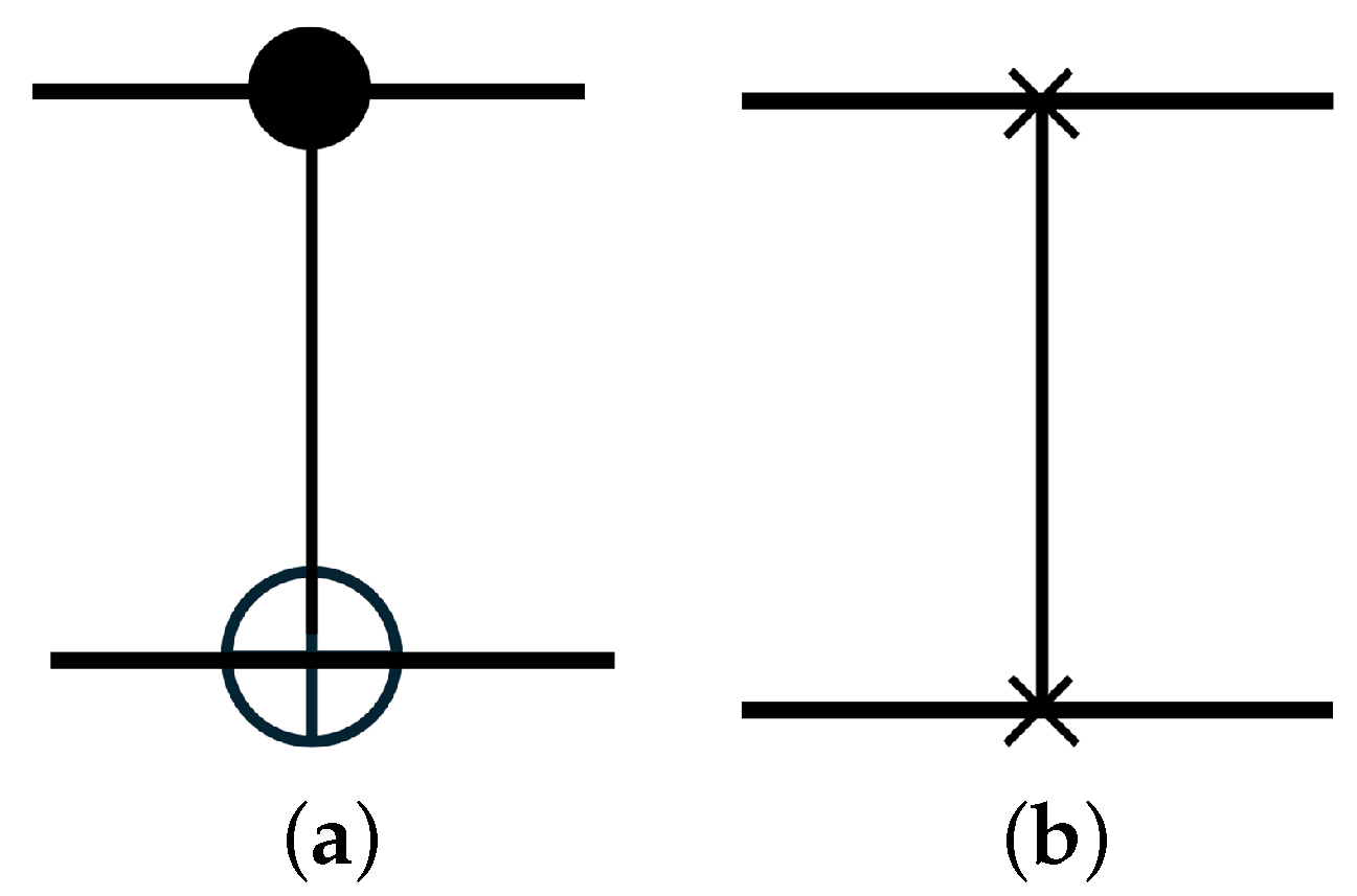

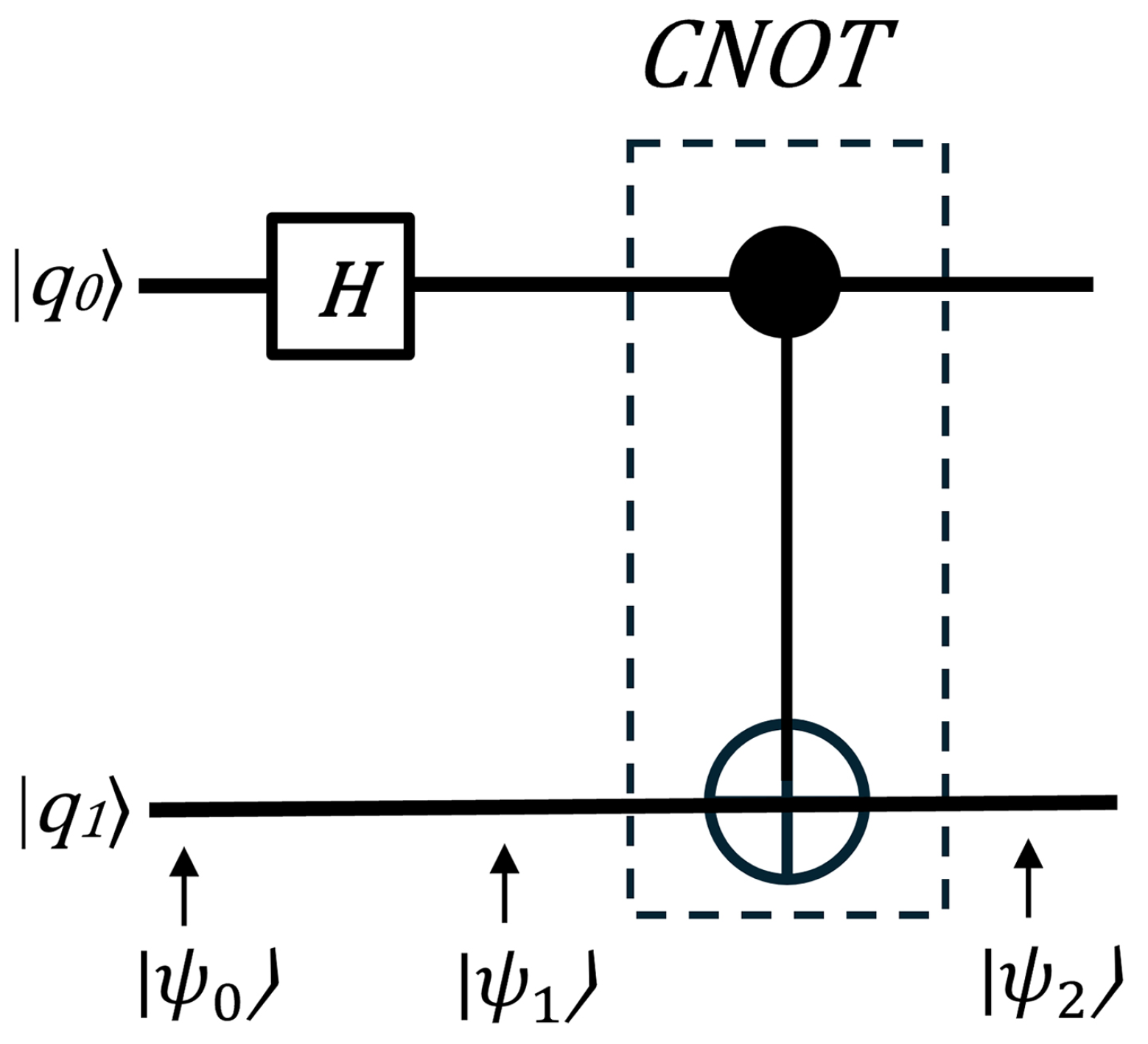
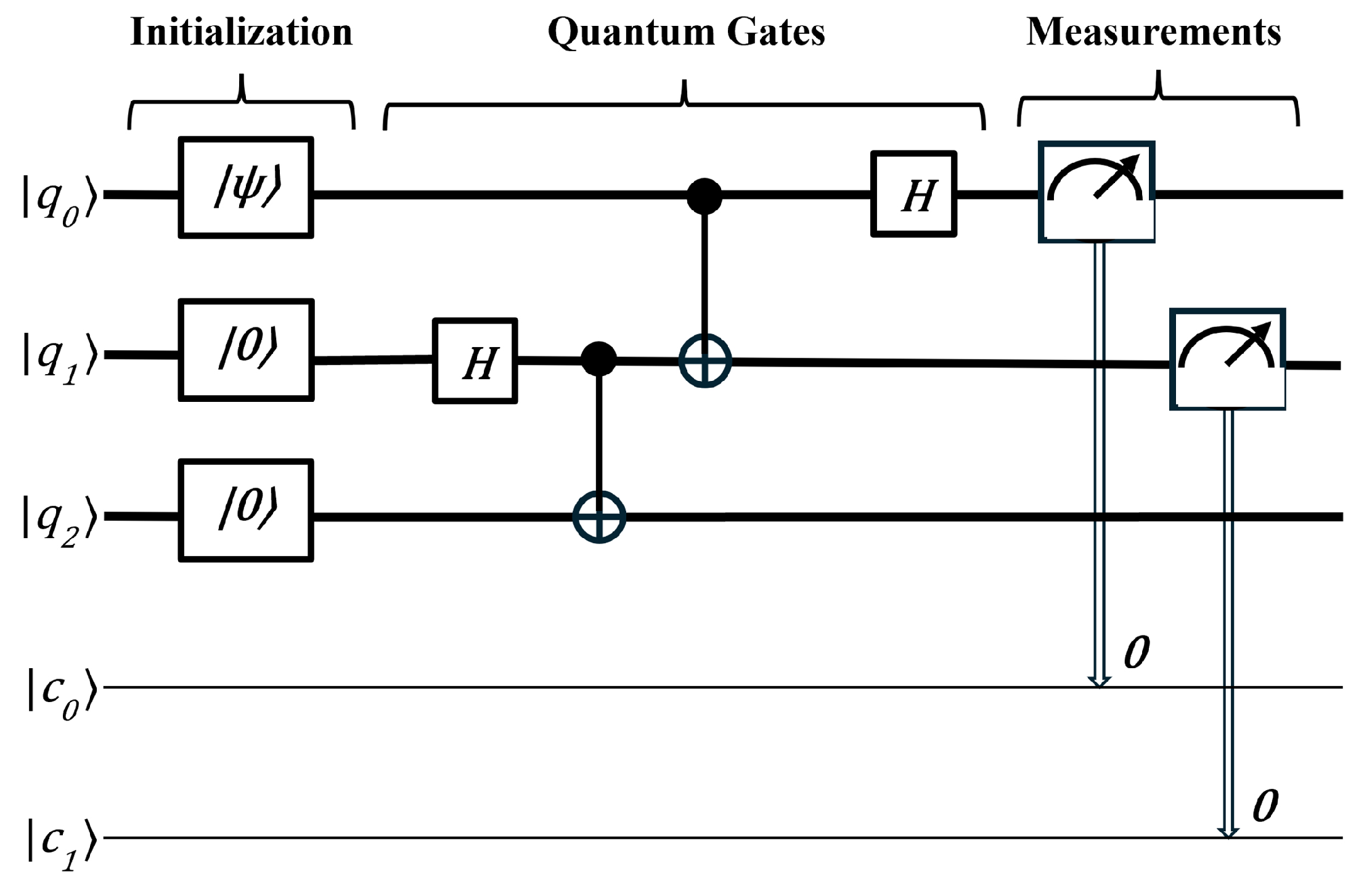
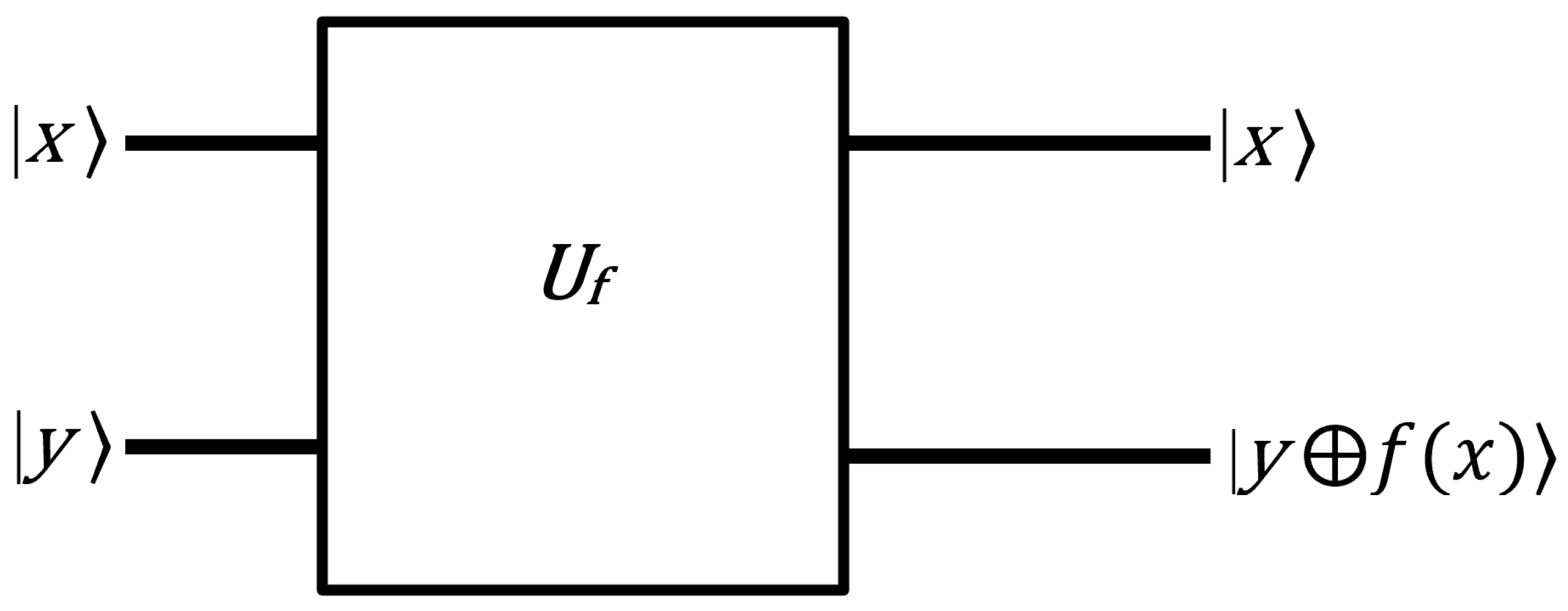
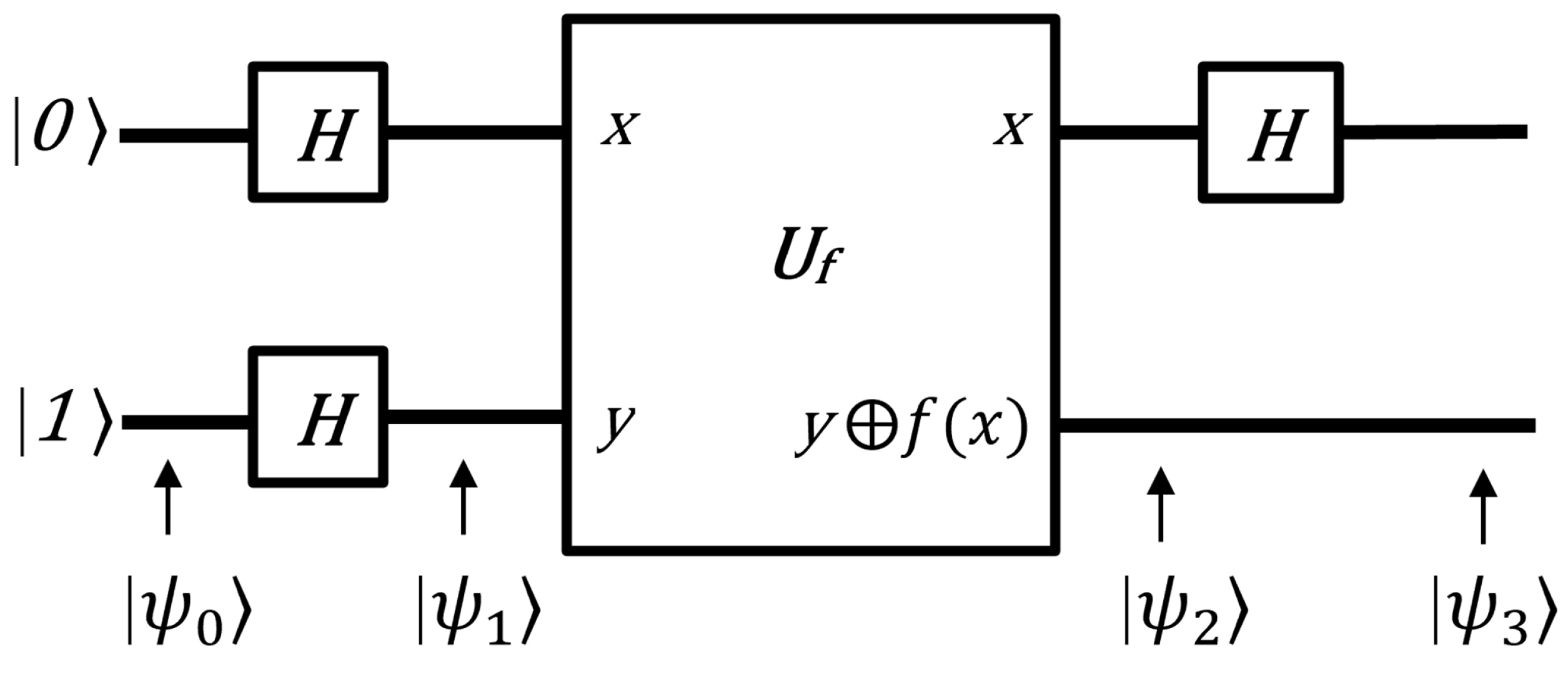

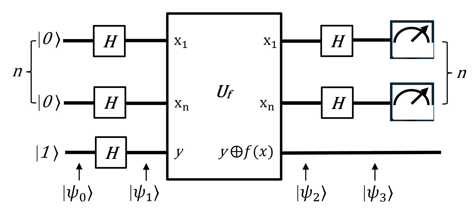


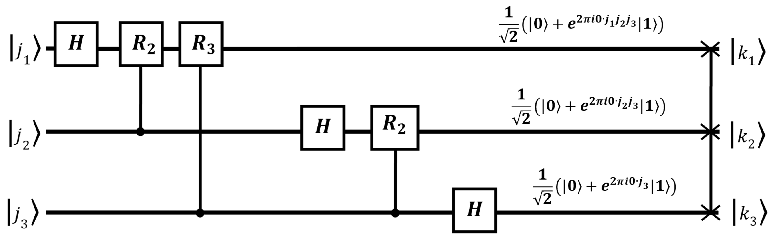
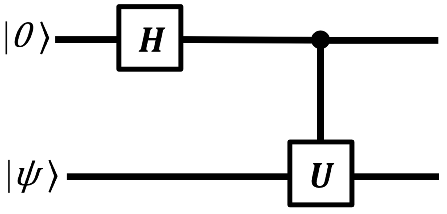
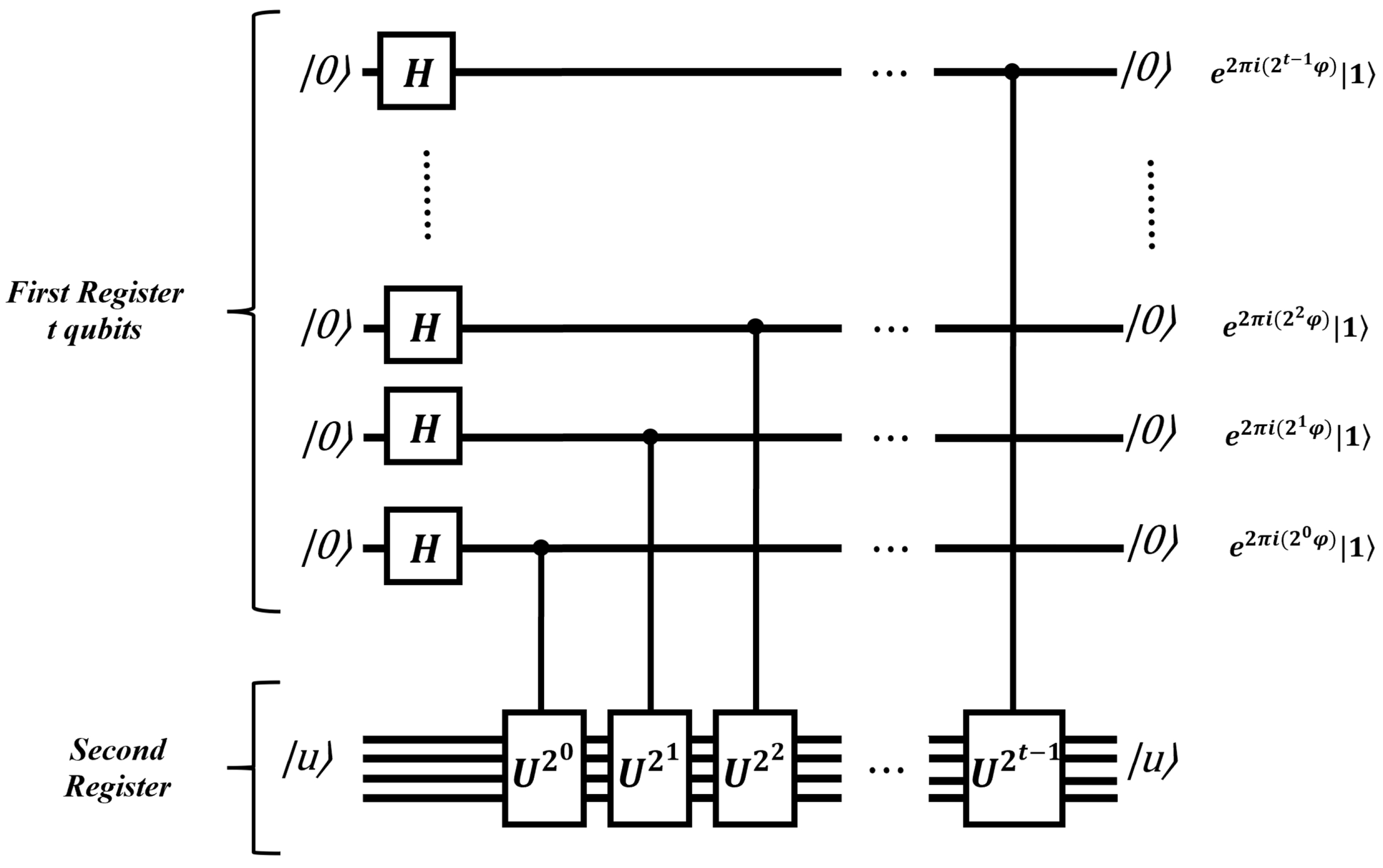
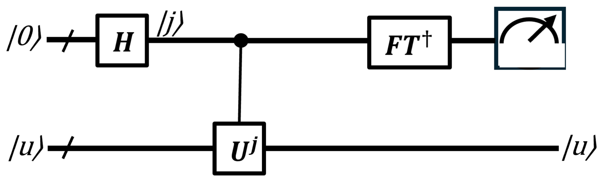

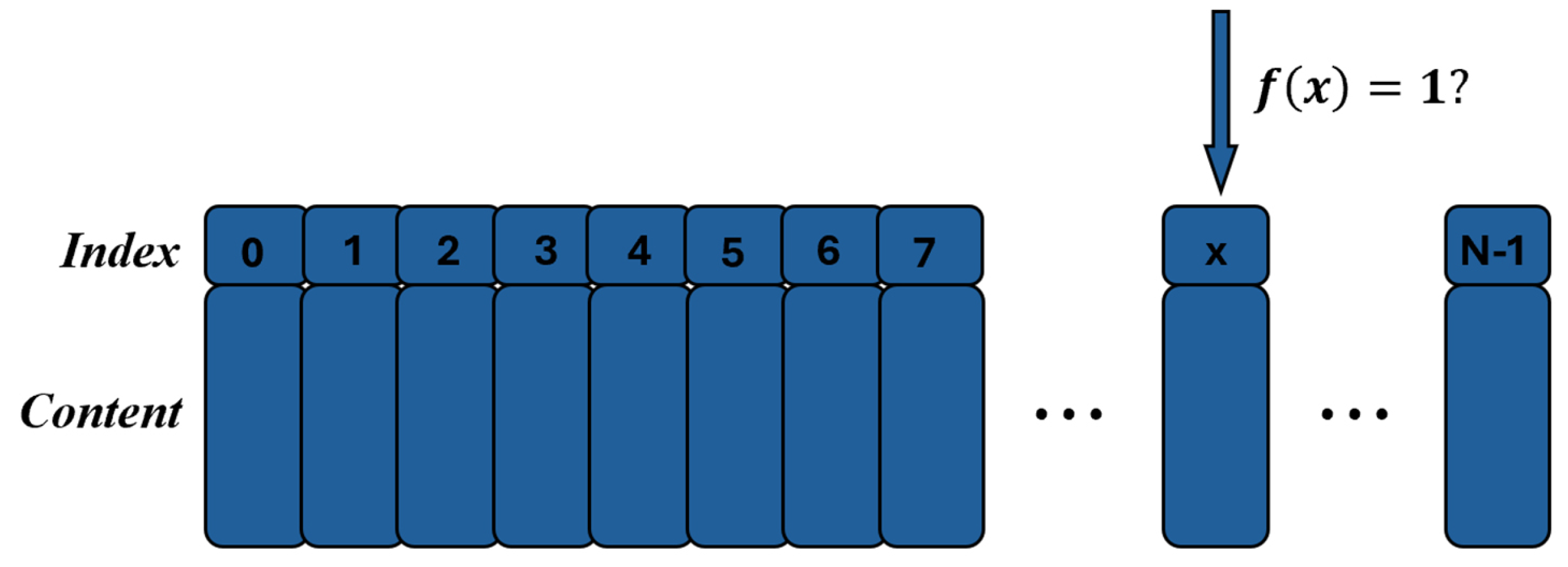
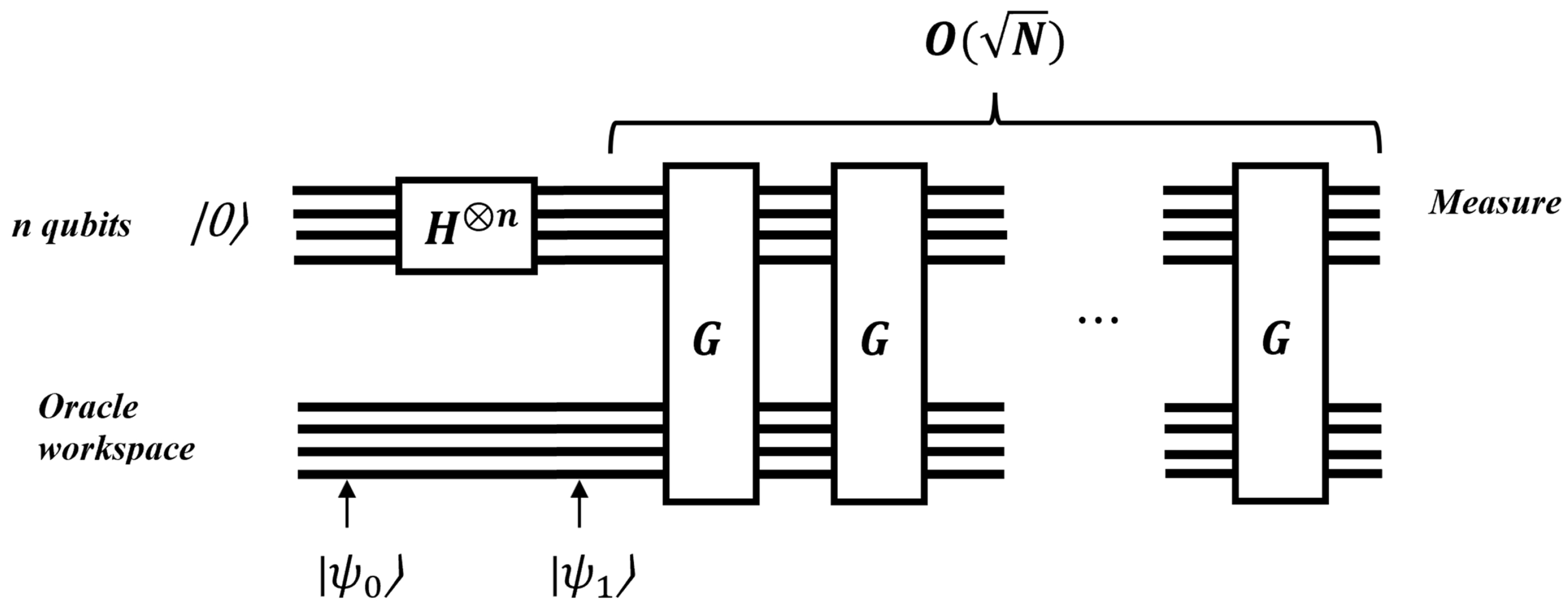
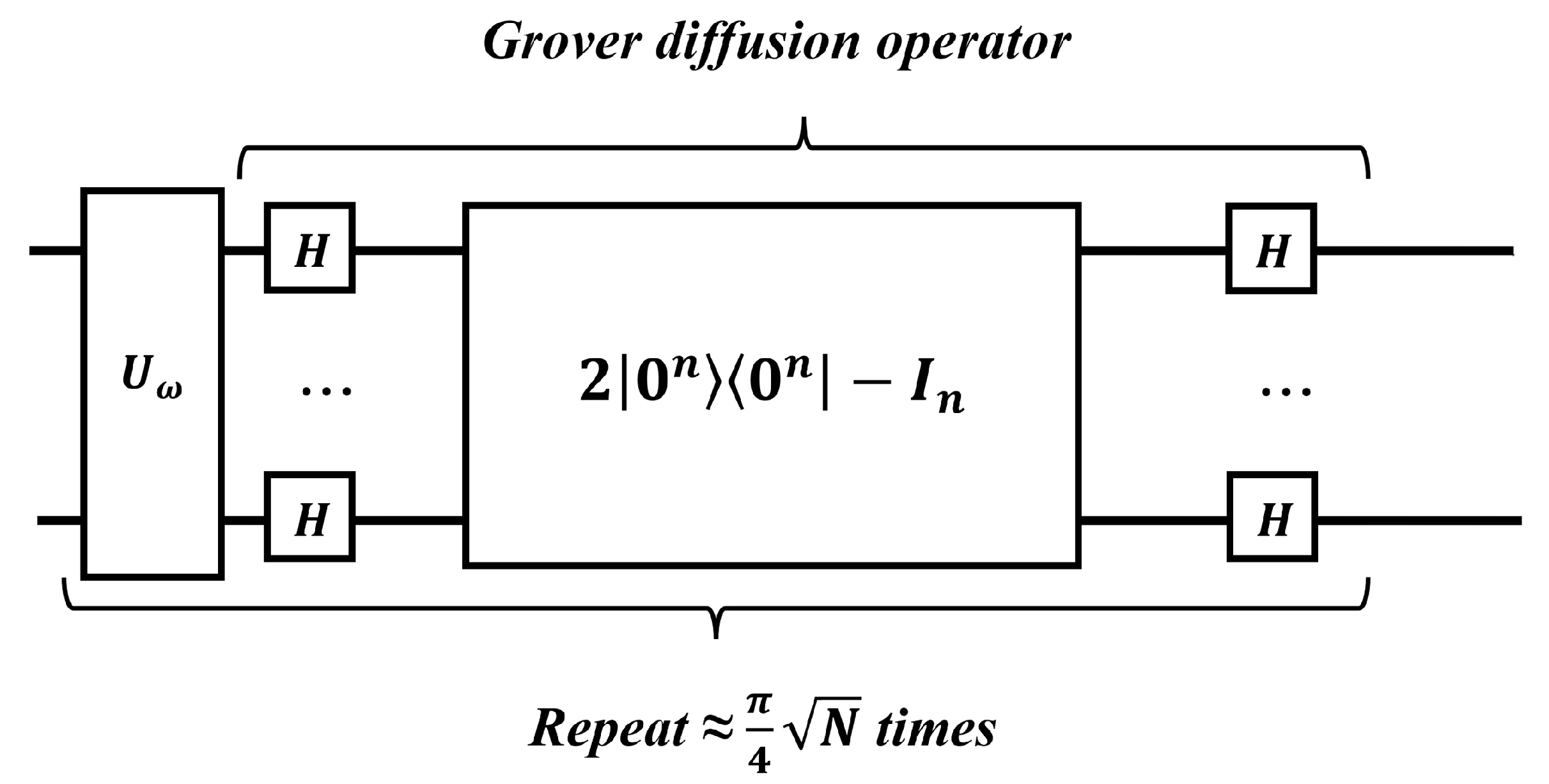

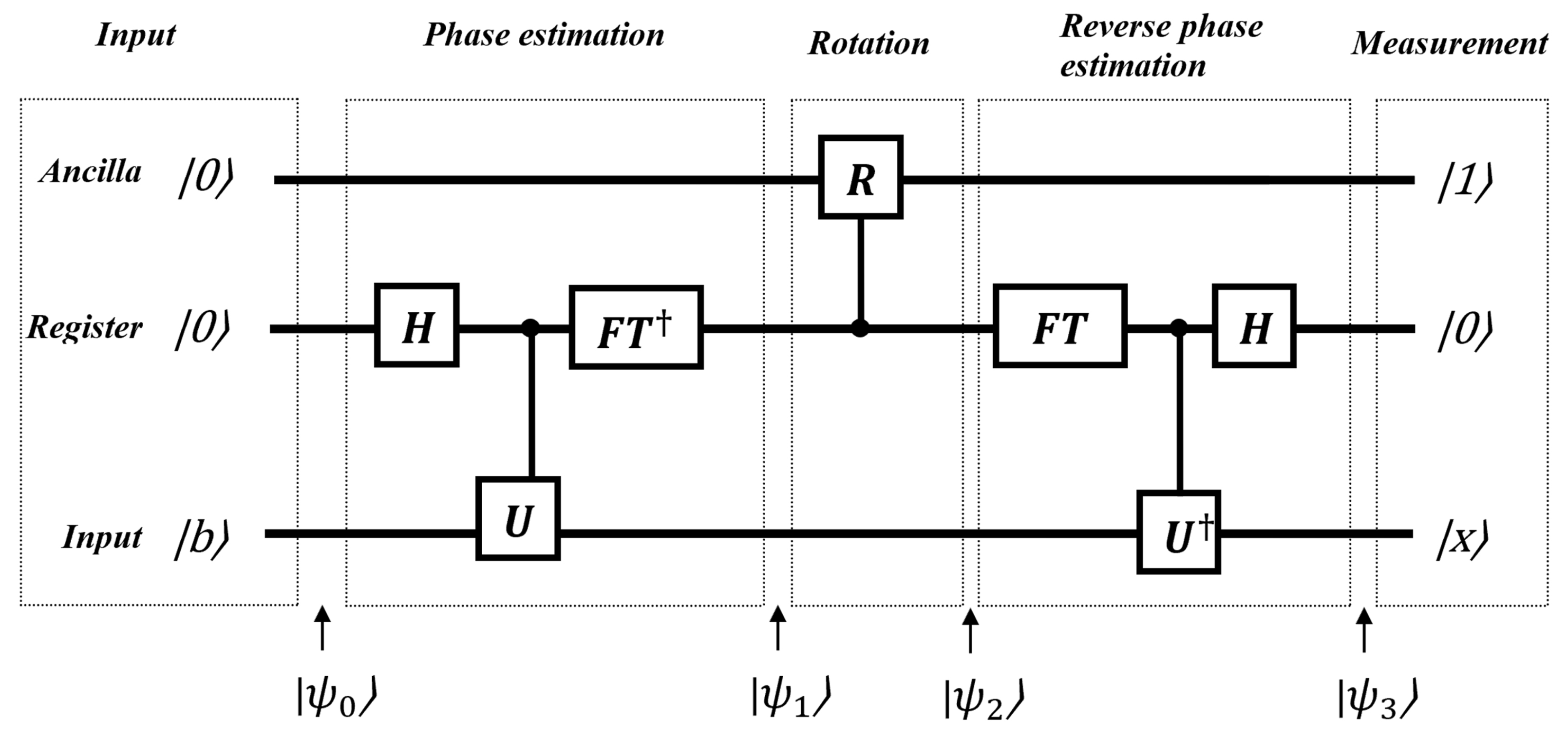
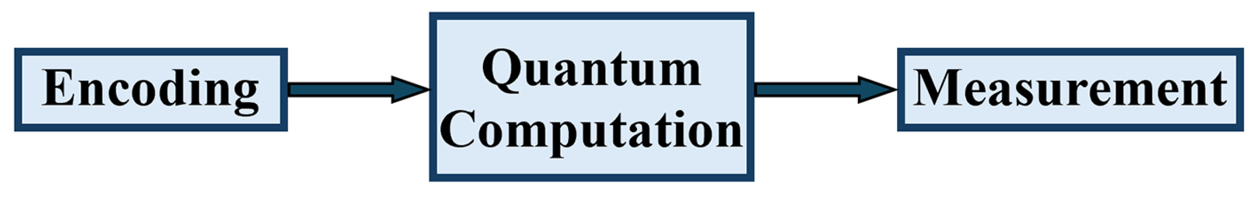
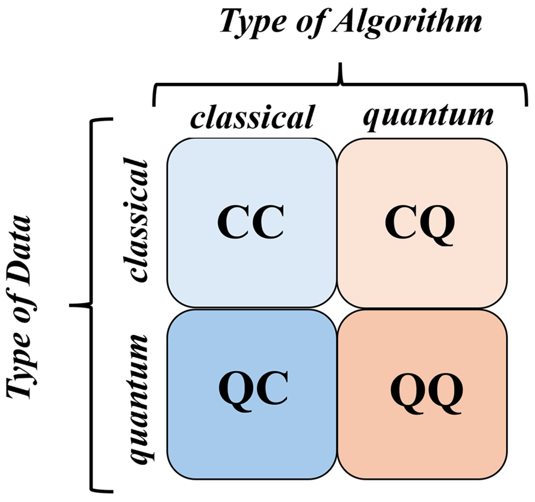
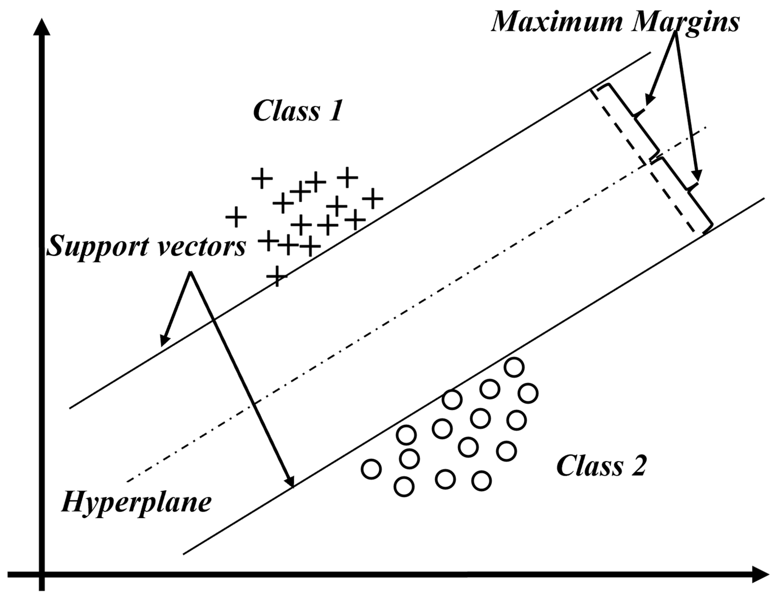

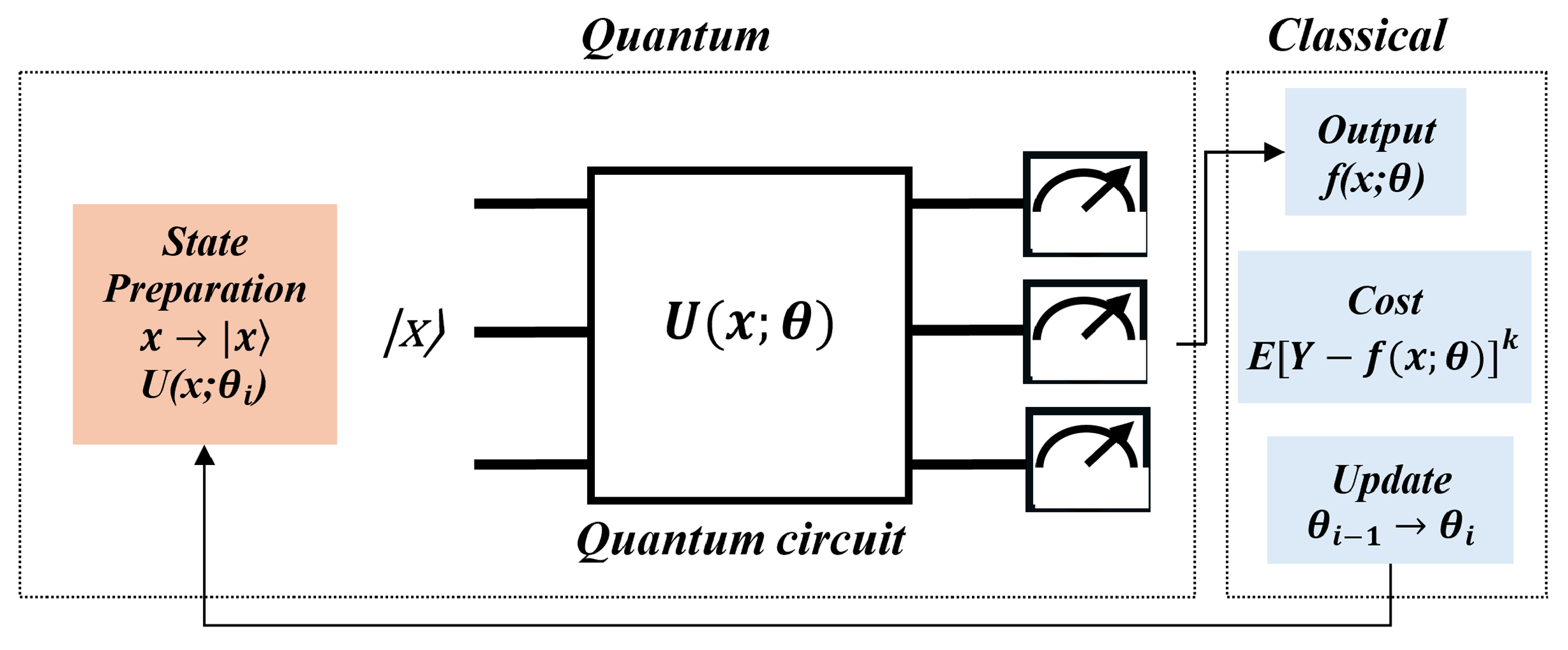
